Technical note: Rapid assessment of drivers and air quality effects of regional daily changes in air pollutant emissions based on near-real-time techniques

Fast and timely estimation of air pollutant emissions is critical for understanding the complex sources of air pollution and supporting air quality improvement, while current emission inventory was commonly reported with time lag or coarse temporal resolution. Here we developed a near-real-time approach that calculates the daily emissions of anthropogenic air pollutants, and applied this approach for Jiangsu province, a typical developed region in eastern China. We estimated that the annual total anthropogenic emissions of SO₂, NO_x, primary fine particles (PM_2.5), non-methane volatile organic compounds (NMVOCs), and NH₃ were 246, 727, 298, 1186, and 377 Gg, respectively, for Jiangsu in 2022. Compared to available national emission inventory (MEIC), application of the provincial-level daily emission estimates provided better model performance of PM_2.5 and ozone (O₃) simulation for all seasons (represented by January, April, July and October). The NO_x, SO₂, PM_2.5, and NMVOCs emissions in Jiangsu during April–May 2022 (the period of COVID-19 lockdown in Shanghai) were respectively 8 %, 6 %, 6 %, and 10 % smaller than those in the same period of 2023. Transportation and Industry respectively contributed 89 % of NO_x emission reduction and 93 % of NMVOCs reduction. Combining with machine learning, moreover, we revealed that the changing agricultural NH₃ emissions dominated the variability of daily PM_2.5 concentration, and that off-road transportation contributed substantially to variabilities of both PM_2.5 and O₃ levels. The study proved advantages of incorporation of near-real-time data and machine learning techniques on tracking the fast-changing emissions and detecting the sources of varying air quality.

1 Introduction

Emissions of air pollutants from anthropogenic activity including traffic, industrial plants, and residential and commercial fuel consumption are the main cause of worsened air quality, especially in economically developed regions with dense populations (Sokhi et al., 2022; Zheng et al., 2018). Emission inventory, which contains complete information on magnitude, spatial pattern, and temporal change of air pollutant emissions by sector, is essential for identifying the sources of air pollution and effectiveness of emission controls on air quality through numerical modeling (Zhao et al., 2013; Zhang et al., 2019a). Traditionally, “bottom-up” methodology (i.e., the emissions were calculated for the finest source categories and then aggregated to bigger categories) provides robust time series of emission estimates based on national statistics (An et al., 2021; Crippa et al., 2020; Kurokawa and Ohara, 2020). However, these emission estimates were usually reported with a time lag of at least 3–5 years. The delay reflected the time needed to finalize accurate national statistics (e.g., official energy consumption by fuel type) and that needed to collect and process them for compiling emission inventories (Guevara et al., 2023). As a result, in addition to the inherent uncertainties in emission inventories, this delay can introduce extra uncertainty when these inventories are employed in air quality modeling, as they may miss current emission characteristics (Wu et al., 2024). Such limitation can be greatly exacerbated for periods with big and unexpected emission fluctuations, resulting from temporary actions for major events or public health incidents (Huang et al., 2021; Wang et al., 2025).

To better track the changing emissions for specific events or incidents (e.g., COVID-19 pandemic), researchers have developed alternative methods to obtain the near-real-time emission estimates (Gaubert et al., 2021; Schneider et al., 2022). The objective of these efforts is to understand the driving factors of the changing emissions and their impact on air quality. Real-time activity information with high temporal resolution started to be incorporated in the emission estimation, such as the electricity load and generation data by national transmission system operators, the real-time vehicle flows monitored from navigation applications, and the real-time ship navigational information from automatic identification system (AIS) (Liu et al., 2020a, b; Zheng et al., 2021; Huang et al., 2021; Harkins et al., 2021; Guevara et al., 2021). Although limited availability and huge capacity of these data hinder their full use in emission inventory development, there is a big potential in expanding the data source to improve the capability of capturing the fast-changing emissions.

Currently, studies have been conducted for carbon dioxides (CO₂) emissions and near-real-time data platforms and products have been developed, particularly for well-identified stationary sources such as fossil fuel combustion plants (BEIS, 2022; CBS, 2024; CITEPA, 2024; Carbon Monitor, 2024). Comparatively, achieving near-real-time estimates is more challenging for air pollutants due to the large complexity and variability of their emission processes. A great variety of air pollutants come from a wide range of sources, containing fuel combustion, industrial processes, on-road and off-road traffic, solvent evaporation, and agricultural activities (Xu et al., 2023; Zheng et al., 2020). The emissions can be greatly influenced by many factors and change a lot. Those factors include the human behavior patterns, operating conditions of plants, improved use of manufacturing and pollution control technologies, and/or meteorological conditions (Liu and Yang, 2024; Lei et al., 2023; Geng et al., 2024). Given the strong chemical reactivity and short atmospheric lifetime of many air pollutants, there exist complicated relationships between emissions and air quality, emphasizing the importance of tracking the fast-changing emissions (Liu et al., 2020; Zhao et al., 2020a). Therefore, efforts are still in great need to develop effective approach for estimating the near-real-time emissions.

For the past years, China has substantially enhanced emission control for industrial (e.g., “ultra-low” emission retrofit for selected non-electrical industries) and residential sources (e.g., promotion of advanced stoves and clean coals during heating seasons). Those measures have clearly reduced emissions of many air pollutants, resulting in a 17.2 µg m⁻³ decline of fine particle (PM_2.5) concentration between 2015 and 2020 over the country (Geng et al., 2024). In contrast, the emissions of NO_x and PM_2.5 from passenger transportation respectively grew by 178 % and 152 % from 2019–2022 (Zhang et al., 2023), and the maximum daily 8 h mean ozone (MDA8 O₃) concentrations increased 5.8 % from 2021–2022 for the country (MEE, 2023). The diverse changes in emissions and air quality highlight the necessity to quickly and accurately reveal the drivers of changes in air pollutant emissions and their impact on ambient air quality (Gu et al., 2023). This is particularly important for periods with severe air pollution episodes and unexpected incidents that substantially changed human activities like COVID-19 lockdown, as timely temporary actions to address pollution might be urgently required.

Province serves as a crucial role in air quality management in China. Due to difference in economic and energy structure and atmospheric conditions, local governments often implement diverse strategies and actions to reduce regional air pollution. This results in large variability in both emission and air quality changes across different regions (Liu et al., 2022; Wang et al., 2021). Studies relying on national emission data offer limited guidance in developing emission control measures and assessing their effectiveness in air quality improvement (An et al., 2021). Jiangsu Province, located in the Yangtze River Delta (YRD) in eastern China, is one of most economically developed regions across the country (Fig. S1 in the Supplement). It accounted for 10.2 % of the gross domestic product (GDP) in mainland China (ranking the second place in the country), and 8.1 %, 12.4 % and 11.6 % of coal consumption, cement and crude steel production in 2022, respectively (NBS, 2023). Following the implementation of air pollution prevention measures, the PM_2.5 pollution in Jiangsu has significantly decreased since 2015. However, the development of the petrochemical industry and transportation has led to rapid changes in emissions, making Jiangsu as the province with the highest and fastest growing O₃ concentration in YRD in recent years (Zhou et al., 2017; Wang et al., 2022).

In this study, therefore, we selected Jiangsu as an example to demonstrate the development of near-real-time emission inventory and its application on rapid assessment of air quality. Based on our previous work that incorporated the best available facility-level information to develop a comprehensive provincial emission inventory (Gu et al., 2023), here we constructed an approach driven by real-time activity data from multiple sources. In this study, “near-real-time” refers to two fundamental aspects. First, the emissions were rapidly estimated based on dynamic activity data, with a minimal delay. It greatly bridged the substantial temporal gap between the occurrence of emissions and the release of official statistical data. Second, it refers to high temporal resolution of the emission data. Unlike previous emission inventories that commonly provided monthly or annual average estimates, the near-real-time approach provided daily emission data and thereby captured the short and temporary perturbations of emissions from anthropogenic activities. The pollutants include SO₂, NO_x, primary PM_2.5, NH₃, and non-methane volatile organic compounds (NMVOCs). We then applied the method to obtain the near-real-time emission estimates for 2022–2023, and assessed the driving factors of the short-term emission change during the COVID-19 lockdown period. Finally, we used an Extreme Gradient Boosting (XGBoost) algorithm to explore the relationship between the variability of daily PM_2.5 and O₃ concentrations and their precursor emissions for 2022. The study provides insights for timely design and implementation of air pollution control actions, and can be used for reference for other developed and polluted regions in China and worldwide.

2 Methodology and data

2.1 Framework of near-real-time emission estimation

Figure 1 shows the methodological framework. In our previous study (Gu et al., 2023), we collected, examined, and integrated most available information on emission sources to enhance the completeness and reliability of the provincial emission inventory. All the information, including raw material and energy consumption, product output, and manufacturing and emission control technologies, played an important role in the estimation of near real-time emissions. The specific methods by sector are described in Sect. 2.2. To ensure the robustness of the near-real-time activity data (e.g., traffic indices and CEMS records), a rigorous data quality control protocol was implemented to handle missing values and outliers. Obvious anomalies, defined as values exceeding three standard deviations from the 7 d moving average, were screened and removed. For short-term data gaps (1–2 d), linear interpolation was applied. For longer continuous missing periods (≥3 d), missing values were gap-filled using the historical average of the same day-of-week in the adjacent weeks, adjusted by the regional sector-specific variability.

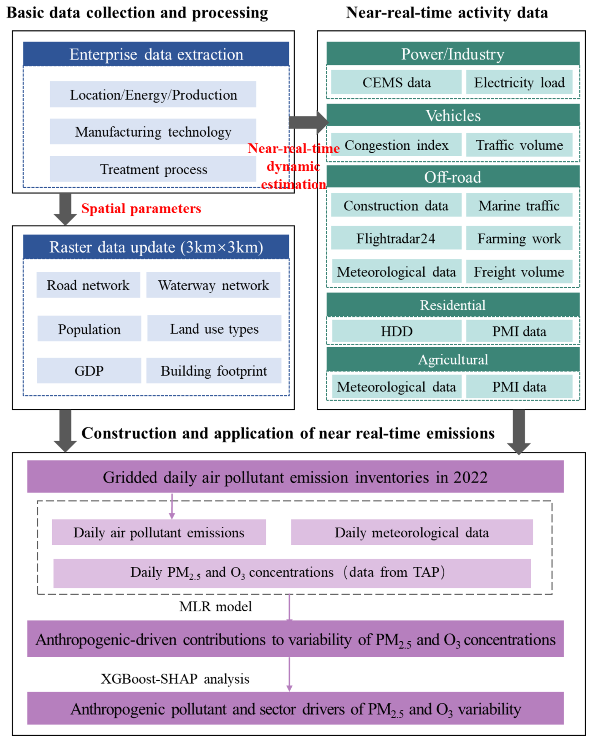
Figure 1 The research framework of near-real-time emission estimation and application in this work.

Furthermore, we improved the spatial distribution of air pollutant emissions. Point sources of power and industrial enterprises were allocated based on their latitudes and longitudes. We further utilized Point of Interest (POI) data from Gaode Map (https://lbs.amap.com/, last access: 22 June 2026) to obtain changes on road/waterway networks, land use, and building footprints. The spatial information is commonly updated every 2–3 months. The use of updated POI data greatly reduced the error of spatial allocation of emissions that may result from the delayed information from the constant spatial proxies (Wang et al., 2017).

2.2 Near-real-time daily emission estimation by sector

This section describes the methods for estimating near-real-time daily emissions for 2022 and 2023. Six major sectors were included (Power, Industrial plant, Vehicles (On-road transportation), Off-road machinery, Residential, and Agriculture), covering most anthropogenic activities. Road and construction site dusts were not contained.

2.2.1 Power plant

Previously we developed a method of applying online measurement data from the continuous emission monitoring systems (CEMS, http://218.94.78.61:8080/newPub/web/home.htm, last access: October 2025) for emission estimation at the unit/plant level (Zhang et al., 2019b). With this basis, we have improved the emission estimation method to enable the stable and continuous acquisition of near-real-time emission data lagged by one month. For the small number of power-generating units without CEMS data, we assumed that their pollutant concentrations in the flue gas were at the average level of units with similar installed capacity (Tang et al., 2019). The emissions were calculated based on the mean hourly flue gas concentration of air pollutant obtained from CEMS and the theoretical flue gas volume of each unit/plant:

$$\begin{array}{}\text{(1)}& {\displaystyle }& {\displaystyle }{E}_{i,j,\text{day}}=C_{i,j,\text{month}}\times {\text{AL}}_{j,\text{month}}\times V_{j,m}^{\mathrm{0}}\times P_{i,j,m,\text{day}}\text{(2)}& {\displaystyle }& {\displaystyle }{\text{AL}}_j={\displaystyle \frac{F_m}{R_m}}\end{array}$$

where E is the emission of air pollutant; i, j and m indicate the specific pollutant species, individual power plant or unit, and fuel type, respectively; C is the monthly average concentration in the flue gas; AL is the activity level (here monthly coal consumption); F is the monthly electricity generation for various fuels, as reported by NBS (2023); R is the fuel consumption rate for power generation, taken from Tong et al. (2021), V⁰ is the theoretical volume of flue gas produced per unit of fuel consumption (Zhao et al., 2010); P is the temporal profile of emissions (the daily to monthly emission ratio), based on the hourly pollutant concentrations and volume of flue gas for the month and specific day.

2.2.2 Industrial plant

With its gradually expanding penetration, CEMS has become able to support near-real-time emission estimation for industrial plants (Tang et al., 2022; Bo et al., 2021). Given its varying coverage across sectors, we have developed a method that can stably estimate the near-real-time emissions at the plant level with a lag of one month. This method classifies industrial plants into three categories based on their CEMS coverage, as described below.

• 1.

  Industrial plants with CEMS information. The method is similar to power plants:

  $$\begin{array}{}\text{(3)}& E_{i,j,\text{day}}=C_{i,j,\text{month}}\times {\text{AL}}_{j,\text{month}}\times V_{i,j,k}^{\mathrm{0}}\times P_{i,j,m,\text{day}}\end{array}$$

  where k denotes the industrial sector; AL is the activity level (here represents monthly product output) as reported by NBS (2023), and V⁰ is the theoretical volume of flue gas produced per unit of product output, which can be found in the technical specifications for the application of emission permits (MEE, 2021).

• 2.

  Industrial plants without CEMS while it was equipped at some plants within the same sector. Sector-level emission factors (emissions per unit of activity level, EF) were calculated using CEMS data from other plants. Monthly emissions were estimated based on the sector-level EF and monthly product output from official environmental statistics. The near-real-time daily emissions were then generated according to the temporal profile of emissions (P) obtained from CEMS installed in other available plants in the sector.

  $$\begin{array}{}\text{(4)}& {\displaystyle }& {\displaystyle }{E}_{i,j,\text{day}}={\text{AL}}_{j,\text{month}}\times {\text{EF}}_{i,k}\times P_{i,j,m,\text{day}}\text{(5)}& {\displaystyle }& {\displaystyle }{\text{EF}}_{i,k}={\displaystyle \frac{E_{i,k,\text{month}}}{{\text{AL}}_{k,\text{month}}}}\end{array}$$

  where EF_i,k is the sector-average emission factor for plants with CEMS for sector k, E_i,k and AL_k are the total emissions from industrial plants with CEMS and their product output, respectively.

• 3.

  Industrial sectors without CEMS data. Emissions were principally calculated based on activity level and emission factor. The activity data were derived based on monthly official statistics reported by NBS (2023). In addition, we analyzed the historical emission source data to trace the evolution of manufacturing and emission control technologies for various sectors, and the emission factors could be calculated for near-real-time emission estimations:

  $$\begin{array}{}\text{(6)}& E_{i,\text{day}}={\text{AL}}_{\text{month}}\times {\text{EF}}_{i,k}\times P_{i,m,\text{day}}\end{array}$$

  where EF represents the emission factor based on the technological evolution of the plant, P is the temporal profile of emissions, based on the fraction of daily electricity load out of the monthly total for specific sector.

2.2.3 Vehicles (on-road transportation)

Daily vehicular emissions were estimated utilizing the International Vehicle Emissions model (IVE) combined with the Gaode live congestion index (Zhou et al., 2019; Kholod et al., 2016). The level of traffic congestion was indicated by the additional time incurred during a trip under congested conditions, expressed as a percentage relative to uncongested conditions (Huo et al., 2022). The Gaode congestion index is available for over 350 cities in China, with a temporal resolution of 5 min (https://report.amap.com/index.do, last access: October 2025). By integrating the congestion index with a Greenshield's traffic density model (Yang et al., 2019), we estimated the traffic volume which serves as a temporal allocation factor to calculate the daily emissions. This approach assumes that vehicular activity data (e.g., mileage and fuel consumption) are accessible, albeit typically with a lag in reporting, as such information is usually provided on an annual basis. Consequently, the near-real-time emissions can be estimated based on the daily variations of congested index and EFs compared to the previous year (Eq. 7):

$$\begin{array}{}\text{(7)}& \begin{array}{rl}{\displaystyle }& {\displaystyle }{E}_{i,m,\text{day}}=\\ {\displaystyle }& {\displaystyle }{\displaystyle \frac{(I_{\text{day,year}}-\mathrm{1})\times I_{\text{day},(\text{year}-\mathrm{1})}^{\mathrm{2}}\times {\text{EF}}_{i,m,\text{day},\text{year}}}{(I_{\text{day},(\text{year}-\mathrm{1})}-\mathrm{1})\times I_{\text{day},\text{year}}^{\mathrm{2}}\times {\text{EF}}_{i,m,\text{day},(\text{year}-\mathrm{1})}}}\end{array}\end{array}$$

In Eq. (7), EF represents the emission factor calculated by the IVE model. The input parameters of IVE, such as vehicle population by type, registration dates, fuel types, and emission standards, can be obtained from the transportation management departments of individual cities. These historical data can be extrapolated to the present date utilizing the vehicle survival curve, thereby bridging any gaps in the current information (Sun et al., 2020). Because official high-frequency traffic activity data are unavailable in near-real-time, we introduced I, the Gaode traffic congestion index, as a dynamic activity scaling factor. This index reflects the comprehensive traffic volume and operational status of the overall road network, allowing us to dynamically scale the baseline emissions into daily-scale trajectories. The index serves as a generalized proxy for total road network activity, and the same scaling factor was applied uniformly for all vehicle types. Although different temporal operational patterns might exist for various vehicle types (e.g., larger volume for trucks during nighttime or on specific freight corridors), obtaining the near-real-time activity information by vehicle type remains a challenge at the provincial level in China. The baseline EF for vehicles in Eq. (7) were derived using the IVE model, which comprehensively accounts for the influences of complex driving conditions, including vehicle speed and engine load. However, continuous recalculation of real-time and speed-dependent EFs on a daily, province-wide scale is computationally intensive and remains as a challenge. For the near-real-time estimation of traffic emissions, therefore, the EFs were treated as baseline constants for 2022, and we predominantly focused on the dynamic adjustment of activity levels and treated them as the primary driving factor for the daily emission fluctuations.

2.2.4 Off-road Transportation

Off-road transportation was divided into five categories: construction machinery, agricultural machinery, marine, railway, and aviation. Emissions from construction machinery were estimated based on assumed daily utilization rates derived from the operating rates of construction sites (Shen et al., 2023; Huang et al., 2021). The daily usage of agricultural machinery was assumed to correlate with the application of nitrogen fertilizers from agricultural sources (see the description of agriculture as below). Emissions from railway, marine and aviation sources were estimated using data from passenger/cargo turnover, individual ports and commercial flights, respectively. These data were obtained from the China Entrepreneur Investment Club (CEIC) (https://www.ceicdata.com.cn, last access: October 2025), Marine Traffic (http://www.marinetraffic.com, last access: October 2025) and Flightradar24 databases (https://www.flightradar24.com/data, last access: October 2025) (Huo et al., 2022; Liu et al., 2020a).

2.2.5 Residential sources

We followed Shao et al. (2023) and developed a Bayesian hierarchical model to estimate daily heating energy consumption by fuel type, based on two primary factors influencing residential energy consumption: temperature and GDP. The daily temperature data were taken from ERA5 products provided by the European Centre for Medium-Range Weather Forecasts (ECMWF) (https://cds.climate.copernicus.eu, last access: October 2025), while GDP from the national statistics published quarterly by the National Bureau of Statistics (http://www.stats.gov.cn/, last access: October 2025). For the months without GDP data, we assumed a linear relationship between GDP and the nighttime light index (Xu et al., 2024), and applied the National Polar-orbiting Partnership Visible Infrared Imaging Radiometer Suite (NPP-VIIRS, https://www.earthdata.nasa.gov/, last access: October 2025) provided by National Aeronautics and Space Administration (NASA) to extrapolate the GDP for those months. We applied the gridded population dataset (1 km×1 km) released by a database of the Chinese Academy of Sciences (https://www.resdc.cn/Default.aspx, last access: October 2025) for 2020. To account for the effect of large-scale population migration, we integrated the Population Migration Index (PMI) developed by Baidu (https://qianxi.baidu.com/#/, last access: October 2025). This index calculates the proportion of incoming migrants relative to the local population.

2.2.6 Agriculture

NH₃ emissions from fertilizer use can be largely influenced by meteorological conditions, soil environment, and farming practices. In our previous study, we quantified NH₃ emissions using dynamic EFs associated with those factors (Zhao et al., 2020b). In this study, we expanded the methodology and estimated NH₃ emissions by using daily EFs. Regarding the baseline activity data for NH₃ estimations, the information was systematically derived from official statistics. For livestock and poultry breeding, we utilized the year-end stock. For synthetic fertilizers, the application amount was calculated as the product of the city-level sown area of cropland and the provincial application rate per unit area obtained from national investigations. To convert these annual totals into dynamic near-real-time estimations, we integrated the temporal allocation of activity data with real-time meteorological conditions. Based on the regional farming database from the Ministry of Agriculture, we tracked the specific growing seasons of major crop types to determine the exact timing of basal dressing and top dressing. By combining the farming cycles with meteorological conditions and high-resolution soil pH databases, we generated the spatiotemporal pattern of NH₃ emissions.

2.3 Air quality modeling

To evaluate the near-real-time emission estimate, we used the Community Multiscale Air Quality (CMAQ v5.1) model developed by US Environmental Protection Agency (https://www.epa.gov/cmaq, last access: October 2025), to simulate the PM_2.5 and O₃ concentrations in Jiangsu. Four months (January, April, July, and October) in 2022 were selected as the simulation periods, with a spin-up time of 7 d for each month to reduce the impact of the initial condition on the simulation. As shown in Fig. S1, three nested domains (D1, D2, and D3) were applied with the horizontal resolutions at 27, 9, and 3 km, respectively, and the most inner D3 covered Jiangsu and parts of the YRD region including Shanghai, northern Zhejiang, and eastern Anhui. The Multi-resolution emission inventory of China (MEIC, http://meicmodel.org.cn/, last access: October 2025) was applied for D1, D2, and the regions out of Jiangsu in D3 (Zheng et al., 2018), and the provincial-level near-real-time emission estimate was applied for Jiangsu in D3. The Carbon Bond Mechanism (CB05) and AERO5 mechanisms were used for the gas-phase chemistry and aerosol module, respectively.

The meteorological field for the CMAQ was obtained from the Weather Research and Forecasting model (WRF v3.4, https://www.mmm.ucar.edu/models/wrf, last access: October 2025). Meteorological initial and boundary conditions were obtained from the National Centers for Environmental Prediction (NCEP, https://psl.noaa.gov/data/reanalysis/reanalysis.shtml, last access: October 2025) datasets. Ground observations at 3 h intervals were downloaded from National Climatic Data Center (NCDC, ftp://ftp.ncdc.noaa.gov/pub/data/noaa/isd-lite/, last access: October 2025). Statistical indicators including bias, index of agreement (IOA), and root mean squared error (RMSE) were used to evaluate the WRF performance (Gu et al., 2023). The discrepancies between simulations and ground observations were within an acceptable range (Table S1 in the Supplement).

We collected ground observation data of hourly PM_2.5 and O₃ concentrations at the 110 state-operating air quality monitoring stations within Jiangsu (https://data.epmap.org/page/index, see the station locations in Fig. S1, last access: October 2025). Correlation coefficients (R), normalized mean bias (NMB) and normalized mean errors (NME) between observation and simulation for each month were calculated to evaluate the performance of CMAQ modeling.

We further compared the modeling performance using the provincial-level near-real-time emission estimates in D3 with that based on MEIC. Since MEIC was currently available till 2020, direct application of MEIC introduce bias from the discrepancy in annual total emissions for different years. To avoid this, we adjusted the annual total emissions of various species in MEIC (for Jiangsu 2020) to perfectly match those of our near-real-time estimates (for Jiangsu 2022), and kept the spatiotemproal distribution of emissions unchanged (referred as “MEIC-revision”). The treatment ensured that any improvement in modeling performance with the near-real-time emission estimate resulted from its optimized spatiotemporal pattern of emissions rather than the total levels.

2.4 Removing meteorological influence on PM_2.5 and O₃ concentrations

To explore the influence of anthropogenic emission changes on the variability of PM_2.5 and O₃ levels in 2022, we removed the impact of varying meteorological conditions by employing a stepwise multiple linear regression (MLR) model (Li et al., 2021). The surface daily concentrations of O₃ and PM_2.5 were taken from the Tracking Air Pollution in China (TAP, http://tapdata.org.cn/, last access: October 2025) with a horizontal resolution of 1 km×1 km (Geng et al., 2021). We incorporated nine meteorological variables from the ERA5 database at a resolution of 0.25°×0.25°, considered as the potential covariates for O₃ and PM_2.5. They were 10 m zonal and meridional wind speeds, temperature, boundary layer height, sea level pressure, cloud cover, precipitation, relative humidity, and dew point temperature. These variables were then scaled to a 3 km×3 km grid system by bilinear interpolation. To prevent overfitting, we conducted MLR with the three most influential meteorological parameters to estimate the variability of daily PM_2.5 and maximum daily 8 h average (MDA8) O₃ concentration for each grid cell. Anomaly (the difference between the raw data and the moving average of 30 d around) of air pollutant concentrations and meteorological factors were used in the model, to exclude the effect of monthly variability. Residuals that cannot be explained by the meteorological variables were assumed to be attributed to anthropogenic emission changes (Li et al., 2020). The results could be interpreted as the sensitivity of air pollutant concentration to the daily emission anomalies from the annual average value.

To evaluate the MLR performance, we collected daily PM_2.5 and O₃ concentrations at the above-mentioned 110 air quality monitoring stations in Jiangsu (Fig. S1), and the R and NMB between observation and MLR were calculated.

2.5 Examining the response of MDA8 O₃ and PM_2.5 concentration to changing daily emissions

2.5.1 XGBoost model

XGBoost model is an advanced and scalable machine learning framework based on gradient-boosted decision trees, widely recognized for its efficiency in handling structured data and modeling complex nonlinear relationships (Requia et al., 2020; Wang et al., 2023). XGBoost excels at processing high-dimensional spatiotemporal datasets, such as gridded emission inventories, by effectively capturing interactions among heterogeneous emission sources and temporal dependencies. Moreover, the inherent interpretability features facilitate seamless integration with explainable AI tools (e.g., SHapley Additive exPlanations (SHAP) to quantify the marginal contribution of each input feature to individual model predictions), enabling rigorous attribution analysis of air pollutant concentration variability (Zhao et al., 2025). To overcome the traditional “black box” limitation of tree-based machine learning models, we utilized the SHAP algorithm to interpret the XGBoost outputs. Based on the algorithm, we were able to explicitly attribute the day-to-day variations in ambient pollutant concentrations to precursor emission changes from specific sectors, thereby drawing physically meaningful and conclusions.

The SHAP value is calculated with following equation:

$$\begin{array}{}\text{(8)}& y_i=y_{\text{base}}+f\left(X_{i,\mathrm{1}}\right)+f\left(X_{i,\mathrm{2}}\right)+\mathrm{\cdots }f\left(X_{i,n}\right)\end{array}$$

where y_i is the predicted value of the model for the ith sample; f(X_i,n) is the contribution of the nth eigenvalue in the ith sample to the final predicted value, with positive or negative representing that the eigenvalue makes the predicted value increase or decrease; and y_base is the baseline value of the predicted outputs for all types of predictions, representing the average prediction results for each category without the influence of any eigenvalue.

2.5.2 Anthropogenic effects on PM_2.5 and MDA8 O₃ variability

The XGBoost-SHAP modeling framework was implemented at the horizontal resolution of 3 km×3 km to capture the emission-concentration relationship. XGBoost regression models were independently trained for each grid cell. January and July were selected as typical months for ambient PM_2.5 and O₃, respectively. Daily time series of 20 pollutant-sector combinations (4 pollutant (SO₂, NO_x, NMVOCs, PM_2.5) × 5 sectors (Power, Industry, On-road (Vehicles), Off-road, Residential) except for tiny On-road SO₂, and agricultural NH₃,) were set as predictors, and anthropogenic-driven variability of PM_2.5 or O₃ concentrations as target variables. Similarly, the emission inputs were treated as anomaly (the difference between the current day's emissions and the moving average of 30 d around). A 10-fold cross-validation was applied (80 % training and 20 % testing), and the bias and correlation coefficient (R) were calculated to evaluate the model performance (Xiao et al., 2018).

SHAP values were calculated for each emission feature using the tree explainer algorithm, quantifying contributions of pollutant-sector combinations to variability of daily anthropogenic-driven concentrations. Note that SHAP values represented the deviation of individual predictions from the baseline expectation. Positive values indicated emission features that elevated pollutant concentrations above the baseline, while negative values indicated features that reduced concentrations below the baseline. Aggregation of daily SHAP values for various pollutant-sector combinations produced the daily-level contribution of total anthropogenic emissions to the changing ambient concentration, and the daily-level contributions could then be aggregated to the monthly level.

3 Results and discussions

3.1 Anthropogenic air pollutant emissions

3.1.1 Total air pollutant emissions in 2022

The total anthropogenic emissions of SO₂, NO_x, PM_2.5, NMVOCs, and NH₃ in Jiangsu for 2022 were estimated at 246, 727, 298, 1186, and 377 Gg (Fig. S2), which were respectively reduced by 17 %, 33 %, 18 %, 7 %, and 11 % compared with those in 2019 (Gu et al., 2023). Note the emissions for multiple years (2015, 2019, and 2022) were estimated with a consistent methodological framework to make reasonbal interannual comparison. Our estimates indicated that the reduction rate of SO₂ emissions was much lower between 2019 and 2022 than that at 53 % between 2015 and 2019. In particular, the emissions from the power sector were estimated to decline only 7 % during 2019–2022. The result confirmed that the abatement of SO₂ emissions have been clearly decelerated following the full implementation of ultra-low emission retrofits, suggesting that the potential of further reduction of SO₂ emissions for power sectors has become more limited. More energy structure adjustment instead of end-of-pipe controls is needed for the sector.

In contrast to SO₂, the emissions of NO_x and PM_2.5 were estimated to decline faster during 2019–2022 than 2015–2019. Industrial sectors contributed largely to these reductions, with the emission declining 27 % and 22 % for NO_x and PM_2.5, respectively (Fig. S2). These reductions reflected expansion of intensified pollution control policies from power to other sectors, particularly the ultra-low emission standards implemented for steel (2019) and cement industries (2020) (https://sthjt.jiangsu.gov.cn/, last access: October 2025). By 2022, Jiangsu province had implemented ultra-low emission retrofits in over 80 % of iron and steel enterprises and approximately 60 % of cement clinker production lines (DEE, 2023). However, slower progress of emission controls in coking, glass, and chemical industries highlighted substantial emission reduction potential in these non-electrical industrial sectors. Meanwhile, the NO_x emissions of transportation were estimated to decline by 41 % from 2019 levels (53 % for light-duty gasoline vehicles), driven mainly by the nationwide implementation of China VI vehicle emission standard and increasing penetration of renewable energy vehicles.

NMVOCs, as critical precursors of both secondary PM_2.5 and O₃ formation, exhibited a slower decline in emissions and have emerged as the priority of emission controls in Jiangsu (Fig. S2). Industrial activities dominate NMVOCs emissions in Jiangsu, contributing 68 % of the provincial total emissions. It resulted from the heavy dependence of the province on chemical industries. For example, the province accounted for over 40 % of national pesticide active ingredient and dye production. Notably, more than 60 % of small-scale chemical enterprises persisted in utilizing solvent-based coatings, inks, and adhesives with high-VOCs content (Simayi et al., 2022; Hu et al., 2024). Furthermore, recent expansions in solvent consumption and chemical output within large-scale enterprises along the Yangtze River have largely offset the emission reductions through improvement of manufacturing and pollution control technologies (Li et al., 2019). Consequently, intensified emission controls should be urgently required for targeting key industrial sectors and critical regions for NMVOCs reduction. Agricultural NH₃ emissions in Jiangsu have experienced a decline of 14 % during 2019–2022, primarily attributed to reduced nitrogen fertilizer usage. However, the absence of effective NH₃ control measures prevented further substantial reduction of emissions for the sector (Zhou et al., 2023; Zhao et al., 2022).

3.1.2 Daily emission variability for air pollutants in 2022

Figure 2 show the daily variability of total and sectoral emissions of various pollutants (SO₂, NO_x, PM_2.5, NMVOCs, and NH₃) in 2022, respectively (the time series of emissions (NO_x as an example) for all the involved source categories are provided in Fig. S3). The results revealed distinct seasonal emission patterns of air pollutants driven by anthropogenic activities and/or meteorological conditions.

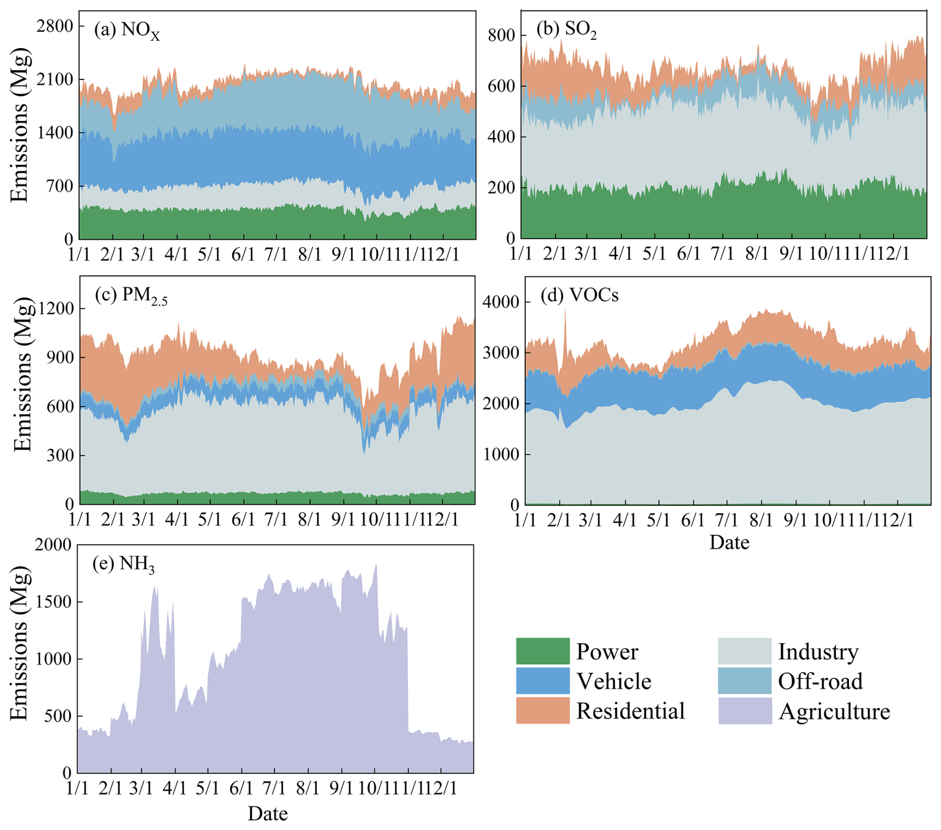
Figure 2 Daily emission estimates of anthropogenic air pollutants by sector for Jiangsu Province in 2022. (a) NO_x; (b) SO₂; (c) PM_2.5; (d) NMVOCs; (e) NH₃.

The emissions of SO₂ and primary PM_2.5 followed the seasonal patterns of fossil energy consumption (Yun et al., 2021), with clear peaks in winter (from December to February) associated with the substantial coal combustion for residential heating and elevated industrial energy demand (Geng et al., 2021; Zhan et al., 2023). Regarding NO_x, transportation has become the primary contributor to the emissions along with improved emission controls from the power and industrial sectors. Following the lifting of COVID-19 lockdown since June 2022, moreover, residents exhibited a strong desire to travel, which enhanced the emissions from transportation. Compared to the spring (from March–May), NO_x emissions from transportation increased 12 % during the summer (from June–August), consistent with the elevated population mobility (Fig. S4). Additionally, the NO_x emission peak in March reflected the resumption of industrial production and construction activities after the Chinese New Year. The area of construction for residential and commercial buildings increased 56 % from February–March, with these activities heavily dependent on diesel-powered machinery (Yang et al., 2015; Cliff et al., 2023). The NMVOCs emissions were the largest in summer. Enhanced volatilization of solvents and industrial chemicals by the warmer temperatures resulted in a 22 % growth of summer emissions compared to spring. Similar to NO_x, the NMVOCs emissions in March rebounded with a 17 % growth compared to February, reflecting the resumption of coating, printing, and petrochemical industries. For NH₃, the highest emissions in March and September were predominantly driven by the intensive spring sowing and autumn farming seasons. In contrast, although the total fertilizer amount decreased in summer (mainly limited to top dressing for specific crops like paddy rice), the high temperature in summer together with top dressing greatly elevated the NH₃ volatilization rates, resulting in peak emission factors that kept the emissions at a high level.

Notably, the province has made great efforts on reducing emissions during the period with heavy pollution weather (DEE, 2022). The restriction measures included alternating operations of energy-intensive industrial plants, such as cement, steel, and glass production, in order to reduce the total production level and energy consumption during the period. Furthermore, industrial parks were required to temporarily shut down or to reduce the load of coal-fired boilers to mitigate regional precursor emissions under the unfavorable meteorological conditions. Compared to August 2022, mandatory restrictions on coal-fired boilers and industrial plants for September resulted in an 11 % reduction of coal consumption for major industrial sectors, leading to a decline of 7 %, 10 %, 15 %, and 12 % for anthropogenic emissions of SO₂, NO_x, PM_2.5, and NMVOCs, respectively. This demonstrated the effectiveness of pollution control measures conducted by the government on counteracting pollution episodes around August and September, despite persistent meteorological challenges (Wang et al., 2023). However, subsequent emission rebounds in winter for SO₂ (+24 % compared with those in Autumn) and PM_2.5 emissions (+19 %) underscored the limitation of seasonal control strategies for combustion-derived pollutants, emphasizing the imperative for clean energy promotion to achieve sustainable emission abatement.

In April 2022, a great reduction in air pollutant emissions was estimated. Compared with March, the emissions of SO₂, NO_x, PM_2.5, and NMVOCs decreased by 11 %, 8 %, 6 %, and 12 % respectively. This abrupt decline was temporally associated with the COVID-19 induced lockdown implemented in Shanghai (28 March–1 June 2022). The lockdown substantially disrupted industrial production, transportation activities, and daily routines in neighboring Jiangsu Province. The results showed that short-term public health incidents exerted profound impact on air pollutant emissions (Zhang et al., 2024; Ma et al., 2023).

3.1.3 High-resolution maps of air pollutant emissions

Based on the real-time geospatial information from the POI system (e.g., quarterly updated road networks, land use types, and monthly revised construction sites), we achieved the evolving spatial pattern of daily air pollutant emissions with a horizontal resolution of 3 km×3 km. Figure 3 presents the spatial distribution of daily average emissions of major sectors in Jiangsu Province for 2022. We selected NO_x as an example to illustrate the sector heterogeneity. The NO_x emissions from power, industrial, vehicle, off-road transportation and residential sources in Jiangsu were calculated at 144, 109, 247, 183 and 45 Gg respectively. Aviation emissions (less than 1 % of total NO_x) were excluded due to their tiny contribution to the total emissions.

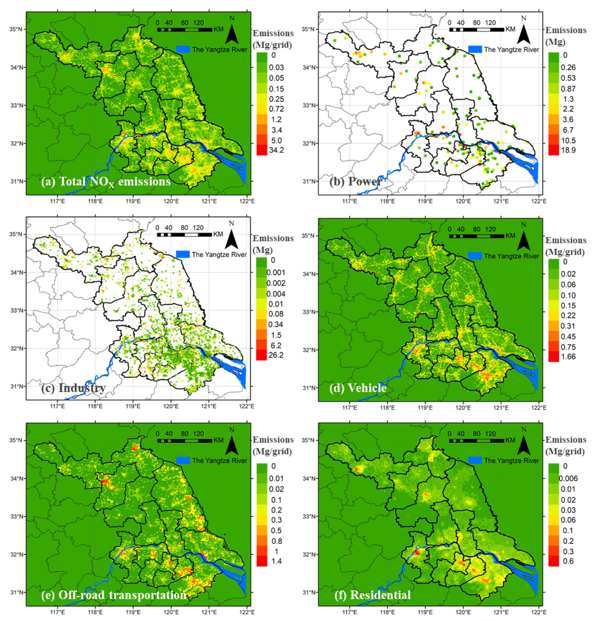
Figure 3 Spatial distribution of anthropogenic NO_x emissions for Jiangsu Province in 2022 with a horizontal resolution of 3 km×3 km. (a) Total emissions; (b) Power; (c) Industry; (d) Vehicle; (e) Off-road transportation; (f) Residential. The map data provided by Resource and Environment Data Cloud Platform are freely available for academic use (http://www.resdc.cn/data.aspx?DATAID=201, last access: 15 October 2025), © Institute of Geographic Sciences & Natural Resources Research, Chinese Academy of Sciences.

The spatial pattern of emissions was closely associated with corresponding anthropogenic activities. Agricultural machinery emissions were predominantly located in northern agricultural zones and coastal areas, correlating with the spatiotemporal distribution of farming activities. In contrast, emissions from other sources were more concentrated in the southern cities, especially along the Yangtze River with the most abundant power and industrial plants. The NO_x emissions from five cities in southern Jiangsu (Nanjing, Suzhou, Wuxi, Changzhou, Zhenjiang) accounted for 59 % and 63 % of provincial power and industrial emissions, respectively. On-road transportation emissions demonstrated a strong dependence on the road network. Nanjing and Xuzhou, as critical national railway transportation hubs, contributed 24 % and 13 % of provincial NO_x emissions from railways (Wang et al., 2016). In addition, Suzhou contributed 29 % of provincial marine emissions, attributed to its pivotal role in Yangtze River Delta inland waterway logistics (Shen et al., 2021). Unsurprisingly, the residential NO_x emissions were closely correlated with the population density.

3.1.4 Assessment of monthly variability

Figure 4 compares the monthly distributions of SO₂, NO_x, and PM_2.5 emissions estimated in this study with those in MEIC, as well as those of provincial averages of ambient concentrations of corresponding species obtained from the state-operating observation sites in Jiangsu. Due to the unavailability of MEIC for the year 2022, we used the result for 2020 instead.

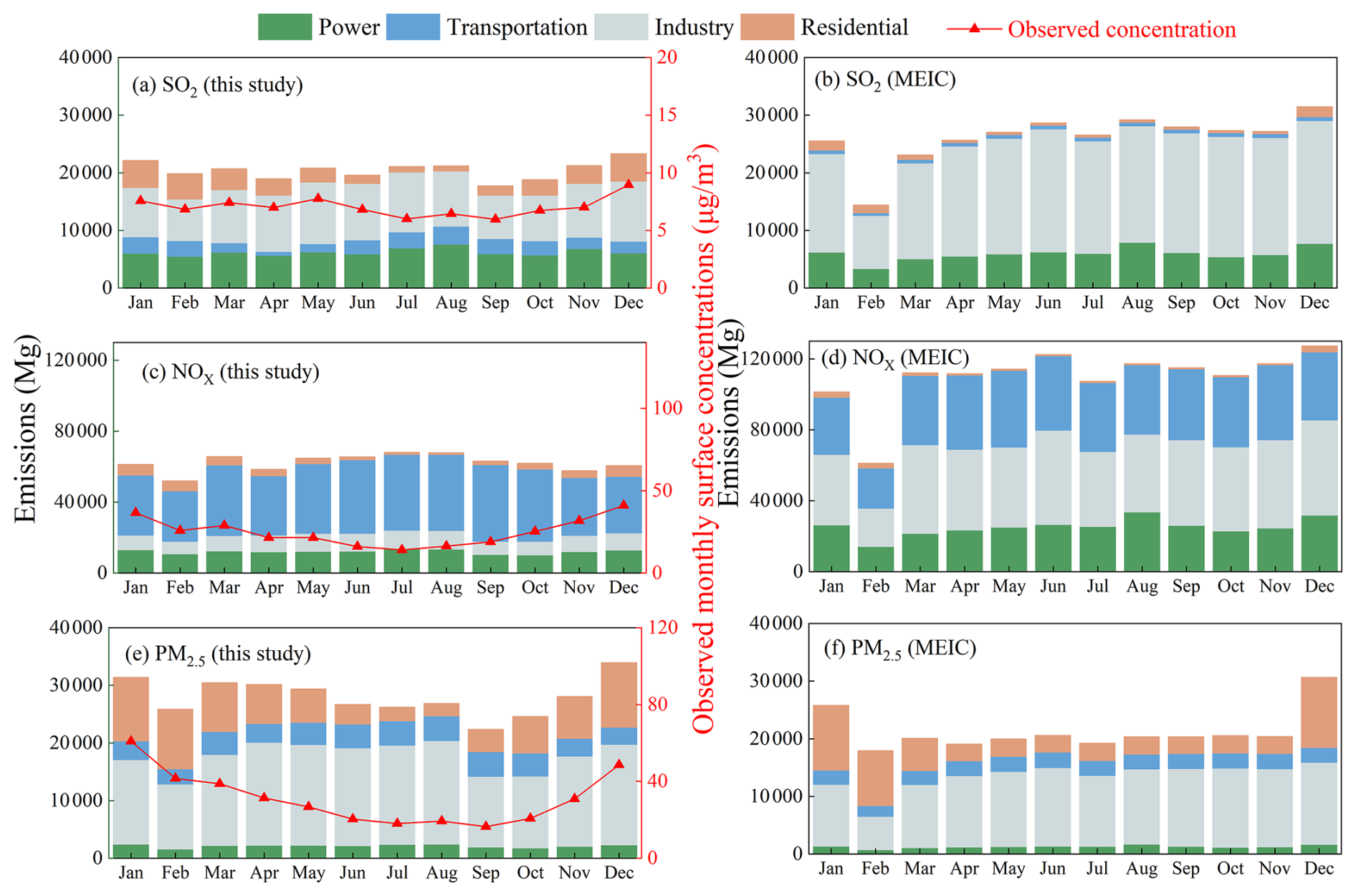
Figure 4 The monthly air pollutant emissions for Jiangsu Province in 2022 estimated in this study (a, c, e) and in national emission inventory (MEIC; b, d, f). The emissions of SO₂ (a, b), NO_x (c, d) and primary PM_2.5 (e, f) are contained. The red lines with triangles represent the observed monthly surface concentrations of corresponding air pollutants.

For SO₂ (Fig. 4a) and PM_2.5 (Fig. 4e), similar monthly variation patterns were found between emissions and observed concentrations in Jiangsu. The near-real-time emission estimates effectively captured the short-term fluctuations in anthropogenic activities, including the abrupt reduction in April associated with the COVID-19 lockdown and the seasonal change from the temporary pollution control measures in autumn. While ambient concentrations were influenced by meteorology and secondary formation as well, the relatively long atmospheric lifetimes of SO₂ and PM_2.5 (typically several days) allow them to reflect the impact of primary emission variations. These results partly justified the capability of the approach to track the effect of changing anthropogenic activities on air pollutant emissions. In contrast, the highly reactive nature and shorter atmospheric lifetime of NO_x resulted in a decoupling between its emissions and ambient concentrations. We found contrary monthly distributions between NO_x emissions and the observed NO₂ concentrations (Fig. 4c). The largest emissions were estimated in summer months but the lowest concentrations were observed for the same months across the year. This inconsistency likely resulted from the following factors. Increased transportation activity in summer, particularly mobility rebound after lockdown, elevated NO_x emissions. Meanwhile, NO₂ was substantially consumed for O₃ formation through rapid photochemical reactions under the intense solar radiation and high temperatures, and its atmospheric lifetime was reduced to merely a few hours. In winter, there was more NO_x accumulation in the atmosphere with weaker photochemical reactions and reduced boundary layer heights (Ding et al., 2015; Wang et al., 2012).

Similar monthly distribution of emissions were found for the national (MEIC) and provincial emission estimates (this work), implying regular patterns of monthly anthropogenic activities could be captured by both inventories. Nevertheless, disparities existed in the overall emission totals and sector distributions between the two inventories. For instance, the contributions of industry to provincial emissions of SO₂ and NO_x were estimated at 45 % and 15 % in this work, greatly different from the MEIC estimation at 72 % and 41 %, respectively. These discrepancies might be attributed to that the national inventory (MEIC) for 2020 has not yet fully included the information of emission control technology upgrades (e.g., ultra-low emission retrofits) in the industrial sector. Taking the sintering process in the steel industry as an example, our facility-level estimations indicated that the average emission factors for SO₂, NO_x, and PM_2.5 were 0.143, 0.228, and 0.037 kg t⁻¹, respectively, much lower than the recommended values of 1.34, 0.55, and 2.52 kg t⁻¹ from the guidelines for development of national emission inventory (He et al., 2018).

Substantial discrepancies were revealed for off-road transportation of SO₂ emissions. The provincial SO₂ emission estimate from marine (12 877 Mg yr⁻¹) were almost three times of that by MEIC (4690 Mg yr⁻¹). As a major freight hub in the eastern coastal region of the country, Jiangsu Province played a pivotal role in marine transportation, and approximately 60 % of vessels utilized heavy oil with high-sulfur content as fuel (Dong et al., 2025). Application of national average EFs for the sector might lead to underestimation in emissions. Furthermore, the national inventory ignored the emissions from passing vessels at ports. Inclusion of such vessels would increase the SO₂ emissions in the Yangtze River Delta region by a factor of 2.3 (Zhang et al., 2017). As power and industrial sectors have gradually completed ultra-low emission retrofits, marine emissions with less stringent controls may become more important in the future, requiring greater efforts on fuel quality improvement and stricter emission controls.

3.2 Impacts of short-term lockdown on changes in emissions

From 28 March–1 June in 2022, Shanghai, the largest megacity in YRD and the national center of economy, finance, manufacturing, and maritime trade in China, implemented stringent COVID-19 lockdown measures that suspended intercity mobility and industrial production and kept only essential logistics. This unprecedented lockdown not only disrupted social and economic activities of Shanghai, but also brought substantial effects for neighboring regions. Jiangsu Province, a highly industrialized region adjacent to Shanghai, experienced severe disruptions across service sectors, manufacturing supply chains, and maritime logistics, resulting in substantial declines in energy consumption, industrial output, and transportation activities. To further quantify the lockdown effect on air pollutant emissions, we conducted a comparative analysis between two periods: the lockdown-affected period (April–May 2022) and the post-pandemic period, the same months one year later (April–May 2023).

The first column of Fig. 5a1, b1, c1, d1 illustrates the variability in daily emissions of NO_x, SO₂, PM_2.5, and NMVOCs in Jiangsu during April–May 2022 (lockdown period) versus 2023 (recovery period), as well as the difference between the two periods. The emission differences (calculated as the relative change compared to the 2023 level) reached 8 %, 6 %, 6 %, and 10 % for these air pollutants, respectively. The most substantial decline in pollutant emissions occurred in April 2022, with a gradually diminishing difference in May. However, the emissions by the end of May 2022 did not reach the level of recovery period in May 2023, reflecting the effect of temporary measures on reducing economic activities even after the lifting of the lockdown. The full economy recovery was delayed until 2023 when pandemic restrictions were completed lifted (Li and Zheng, 2023).

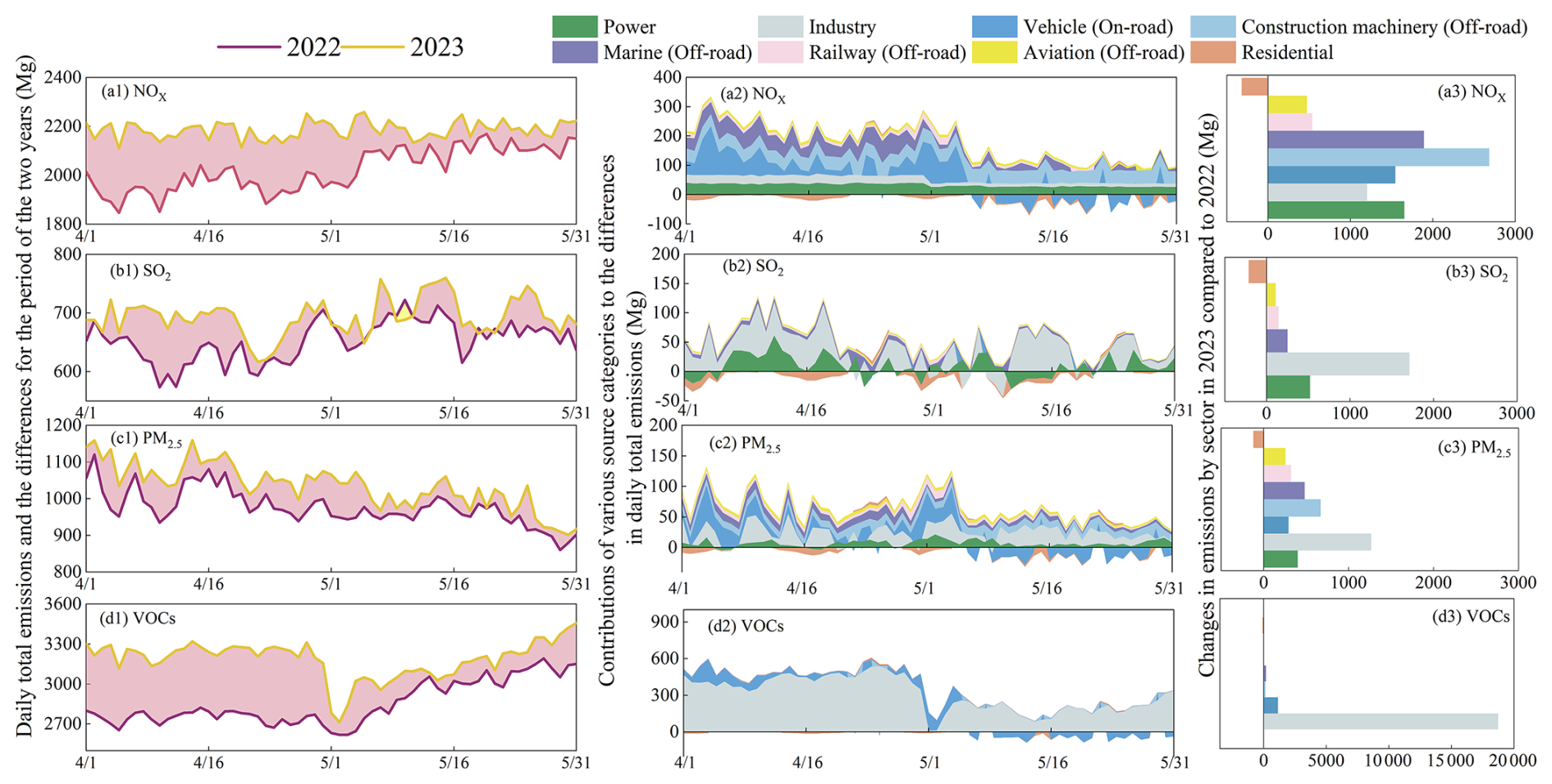
Figure 5 The differences between the emissions of NO_x (a), SO₂ (b), PM_2.5 (c) and NMVOCs (d) in April–May for 2022 and 2023 in Jiangsu Province. The first column illustrates the daily total emissions and the differences for the period of the two years. The second column illustrates the contributions of various source categories to the differences in daily total emissions, and the third column aggregates them for the whole period.

The second and third columns of Fig. 5a2–d2 and a3–d3 illustrate the contributions of various pollution source categories to the differences in emissions between April–May 2022 and 2023. Agricultural production remained basically unaffected by the pandemic, thus the emission changes from agricultural machinery were not included. The total reduction in NO_x emissions was 9970 Mg, predominantly attributed to transportation sources. The sector contributed to over 70 % of the emission reduction, including on-road transportation (15 %), construction machinery (27 %), marine (19 %), railway (5 %), and aviation (4 %). This result is consistent with the findings on the effect of the 2020 COVID-19 lockdown (Lv et al., 2020; Zhao et al., 2020a). However, there was a slight rebound in motor vehicle emissions in May, which could be associated with basic everyday living and working needs. Notably, construction machinery and marine were more affected by the lockdown, attributable to construction material shortages (39 % fewer of constructing and building activities) and disrupted inland waterway logistics (20 % less of port throughput). Compared with transportation, the reduction of NO_x emissions from the power (1955 Mg) and the industrial sector (1202 Mg) were smaller. The decline in industrial electricity demand reduced the fossil fuel consumption and thereby the NO_x emissions from the power sector. During industrial shutdowns and production restrictions caused by the epidemic, frequent start-ups and shutdowns of production and pollution control equipment resulted in a clear decline in NO_x removal efficiency compared with normal operation condition of selective catalytic reduction (SCR) systems. Previous measurements found that the average NO_x removal efficiency of coal-fired units in iron and steel production enterprises decreased from 78 %–61 % (Shao et al., 2023), which to some extent offset the emission reduction effect of industrial sources due to production restrictions.

SO₂ emission reductions predominantly originated from power (521 Mg, 21 %) and industrial sectors (1710 Mg, 68 %). For PM_2.5, transportation contributed 56 % to the total reduction of 3583 Mg, with the contributions from on-road transportation, construction machinery, marine, railway, and aviation accounting for 8 %, 18 %, 14 %, 9 %, and 7 %, respectively. The emission reductions of NMVOCs were estimated at 20 170 Mg. The contribution of industrial sources reached 93 %, largely due to a 64 % decline in crude oil processing in Jiangsu Province compared to 2023, as well as the substantial declines in the production of chemical products (e.g., 27 % less in chemicals fibers and 65 % less in ethylene manufacturing, NBS, 2023). The results emphasized the lockdown impact on petrochemical industries reliant on cross-regional material flows. In contrast, the emissions from residential sector were larger for the lockdown period, with its coal consumption 7 % more than that in recovery period one year later, likely driven by the enhanced heating/cooking demands during mobility restrictions.

In addition, an examination was conducted for exploring the diverse rebounds of emissions for different sectors. Vehicle emissions exhibited a clear growth in May compared to the central lockdown period in April. This early rebound in transportation was likely driven by the gradual recovery of essential logistics and commuting. In contrast, the emissions from industrial sector remained at a greatly suppressed level throughout April and May, without an immediate rebound. This lag in industrial recovery aligned with the socioeconomic condition of YRD, where the regional industrial added value and GDP experienced a substantial decline in the second quarter of 2022, followed by a slow recovery in the subsequent months (JSBS, 2022). Such diversity between sectors indicated that mobile sources and energy supply could respond quickly to the lifting of restrictions, while the recovery of large-scale manufacturing could be more difficult due to complex supply chain realignment.

To further explore the spatial heterogeneity of the lockdown impacts, we conducted a city-level comparative analysis by selecting three representative cities: Suzhou in southern Jiangsu, Nantong in central Jiangsu, and Xuzhou in northern Jiangsu (see locations of the cities in Fig. S1). Suzhou is adjacent to Shanghai, with dense petrochemical and manufacturing industries deeply embedded in regional supply chains. Nantong is located in coastal area and relies heavily on marine logistics and ports. Xuzhou is a city dominated by heavy industries and is farther from Shanghai with less direct lockdown exposure compared to other cities in Jiaingsu.

As a core economic hub deeply integrated with Shanghai's supply chain, Suzhou was greatly influenced by Shanghai lockdown (Table S2). The NMVOCs and NO_x emissions in April–May 2022 dropped 17.9 % (6812 Mg) and 15.2 % (2917 Mg), respectively, compared to the normal level (April–May 2023). This acute decline was co-driven by the near-total freeze of cross-city highway freight, massive operational bottlenecks at major ports, and widespread suspensions of petrochemical and electronics manufacturing. Meanhwile, there existed notable drops in PM_2.5 (−13.0 %) and SO₂ emissions (−9.0 %) from halted construction and industrial fuel use. In Nantong, the moderate declines in NO_x (−9.2 %), NMVOCs (−8.6 %), PM_2.5 (−6.8 %) and SO₂ (−4.9 %) primarily reflected disruptions in regional waterway logistics and slowdowns in general manufacturing. In contrast, the emission reductions in Xuzhou were much smaller around 3 %, attributed to the continous operations of heavy industry to maintain the essential supply chains of industrial economy. These diversities between cities demonstrated the capability of the research framework to track the emission variation due to temporal and/or unexpected events at relatively high spatiotemproal resolution.

In a summary, the results revealed complicated and diverse interventions of public health incidents on energy use and activities for different sectors. The near-real-time techniques developed in this work proved capable to capture the fast response of air pollutant emissions to the short-term measures conducted during unexpected incidents, and to clear identify the driving sectors of emission changes compared to the normal conditions.

3.3 Evaluation of the near-real-time emission estimates with air quality simulation

The near-real-time estimates of provincial emissions were evaluated with air quality simulation with CMAQ. To assess model performance, the observed concentrations of hourly SO₂, NO₂, PM_2.5, and MDA8 O₃ were compared with the simulations based on the provincial-level near-real-time emission estimates and MEIC for the selected four months of 2022, as summarized in Table S3. Overall, the simulation with the provincial emission estimates shows acceptable agreement with the observations, with the annual means of NMB and NME ranging −37.1 % to 24.1 % and 33.7 % to 53.5 % for SO₂, −20.2 % to 27.0 % and 15.9 % to 36.2 % for NO₂, −18.6 % to 10.8 % and 37.5 % to 62.5 % for PM_2.5, and −41.2 % to −23.1 % and 32.7 % to 49.3 % for O₃. The analogous numbers for MEIC were −33.4 % to 25.5 % and 40.9 % to 51.8 % for SO₂, −19.9 % to 35.6 % and 22.3 % to 55.1 % for NO₂, −8.6 % to 25.2 % and 37.5 % to 52.5 % for PM_2.5, and −39.9 % to −28.1 % and 44.3 % to 54.5 % for O₃, respectively. Most of the NMB and NME were within the recommended criteria (−30 % ≤ NMB ≤ 30 % and NME ≤ 50 %, Emery et al., 2017). Better performance was achieved using the provincial emission estimates developed in this work, implying the benefit of applying the refined emission data on high-resolution air quality simulation.

Figures 6 and 7 compares the simulated daily PM_2.5 and O₃ concentrations based on the provincial (this work) and national emission estimates (MEIC) against observations (results for SO₂ and NO₂ are shown in Figs. S5 and S6, while spatial distributions for all the four pollutants are provided in Figs. S7–S10). Compared to MEIC, the provincial-scale emission estimates demonstrated better model performance in capturing the daily variability of pollutant concentrations. The greater correlation coefficients (R) between simulated and observed concentrations based on the near-real-time estimates indicated a remarkable improvement for all the involved air pollutants (Table S3).

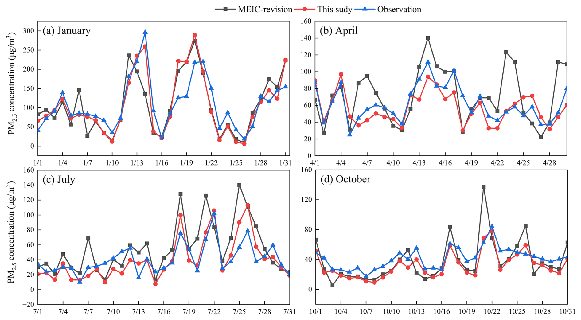
Figure 6 Comparison between the observed daily PM_2.5 concentrations (blue lines) and the simulated concentrations with different emission inventories in Jiangsu Province for January (a), April (b), July (c), and October (d) in 2022. The simulations were conducted using the near-real-time emission inventory developed in this work (red lines) and the revised national emission inventory MEIC (MEIC-revision, black lines). See Sect. 2.3 for the rationale of MEIC revision.

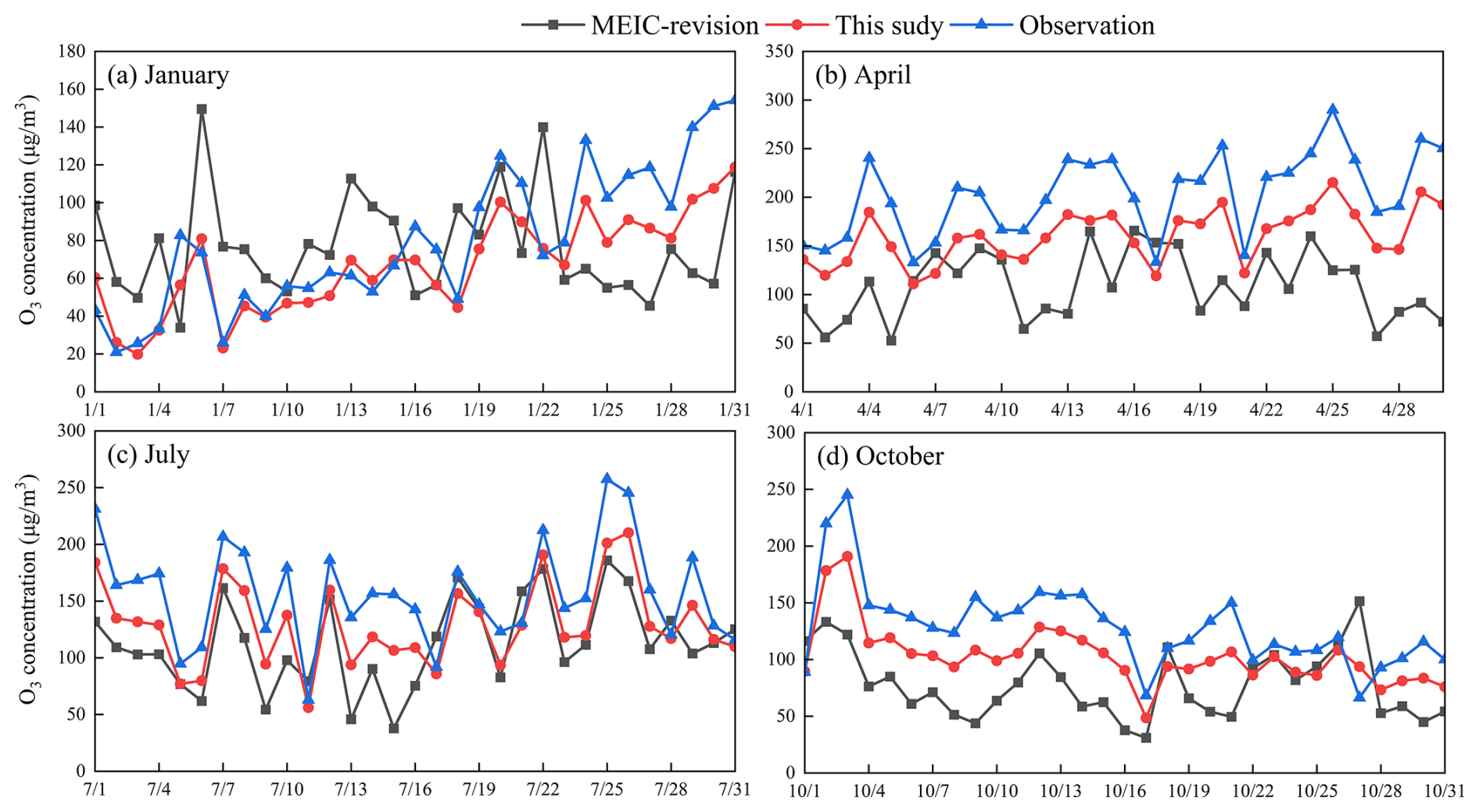
Figure 7 Comparison between the observed daily maximum 8 h average (MDA8) O₃ concentrations and the simulated concentrations with different emission inventories in Jiangsu Province for January (a), April (b), July (c), and October (d) in 2022. The simulations were conducted using the near-real-time emission inventory developed in this work (red lines) and the revised national emission inventory MEIC (MEIC-revision, black lines). See Sect. 2.3 for the rationale of MEIC revision.

Figure 6 compares the observed and simulated PM_2.5 concentrations, and measurable improvement of model performance was achieved with the updated temporal profiles for emissions. Specifically, the NMEs for January, April, July, and October decreased from 37.5 %, 55.3 %, 62.5 %, and 51.3 % to 33.2 %, 29.2 %, 48.1 %, and 42.6 %, respectively. The greatly improved model performance for April 2022 demonstrated the capability of the near-real-time emission data to better capture the influence of temporarily disrupted anthropogenic activities on air quality. During this period, the COVID-19 lockdown in Shanghai severely restricted cross-regional freight transport and industrial operations in Jiangsu (Huang et al., 2021). Compared with previous emission inventories relying on historical temporal patterns, the refined daily emission inventory with near-real-time techniques provided a more realistic representation of the decline in primary aerosols and precursor emissions from heavy-duty vehicles and point sources. Consequently, the simulated PM_2.5 concentrations showed better agreement with observations, with the NMB reduced to −6.6 %. The refined emission inventory also yielded notable corrections for periods with targeted administrative interventions. During the late July period (20–31 July), for example, the NMB for PM_2.5 decreased from 47.3 % with MEIC to 16.1 % with the near-real-time emission data, and the simulated mean concentrations dropped from 76.4–60.2 µg m⁻³, much closer to the observed 52.0 µg m⁻³. This improvement was likely attributable to the inventory's dynamic response to official electricity rationing policy. Driven by extreme summer heat waves and power grid stress, local governments mandated load reduction measures for energy-intensive facilities (Wei et al., 2020), causing an irregular drop in industrial emissions that may not be tracked in previous inventories. Similarly, the clear overestimation with MEIC for October was effectively mitigated. The refined emission data appeared to better reflect the benefit of stringent control measures implemented for preventing the heavy haze pollution in autumn and winter (Jiang et al., 2023).

Figure 7 presents the observed and simulated O₃ concentrations. Compared with MEIC, the NMEs with the near-real-time emission data for January, April, July, and October decreased from 51.4 %, 54.0 %, 44.3 %, and 54.5 % to 49.3 %, 41.1 %, 32.7 %, and 34.6 %, respectively. The updated emission data could have modulated the simulation of non-linear photochemical processes. In January when weak solar radiation generally limits photochemical O₃ production, NO_x titration often acts as a dominating mechanism. The simulation with MEIC underestimated NO₂ by 37.4 %, and it potentially contributed to a 36.0 % overestimation of O₃ due to insufficient chemical scavenging. With the NO_x emissions 12 % higher than MEIC during the January, the near-real-time emission inventory resulted in a more reasonable simulation of the titration effect. The enhanced chemical sink reduced the O₃ NMB to −23.1 % and improved the R² from 0.30–0.66. For April, the NO_x emissions were 15.9 % lower in the real-near-time inventory than MEIC. Such a reduction in NO_x could effectively weaken the titration inhibition, and it likely allowed the model to better track the accelerated accumulation of O₃ driven by increasing spring solar radiation. Simulation with the refined emission data yielded a growth of 1.72 µg m⁻³ for the month, much closer to the observation (2.59 µg m⁻³) than that with MEIC (0.33 µg m⁻³). Furthermore, there existed substantial correction of O₃ underestimation in October, with the NME reduced from 54.5 % to 34.6 %. Such improvement resulted potentially from the better simulated aerosol-radiation feedback. As mentioned earlier, specific measures were conducted during autumn and winter in Jiangsu to prevent heavy haze pollution. The emission abatement resulting from those measures were captured by the near-real-time techniques, facilitating a lower aerosol loading in CMAQ simulation compared to that with MEIC. This could theoretically elevate photochemistry process and accelerate O₃ production, partially bridging the gap between simulation and observation. In contrast, MEIC did not fully include the local pollution control measures for specific seasons, and the relatively high aerosol loading from simlation might have overly suppressed photochemical O₃ formation by scattering and absorbing actinic flux (Zhao et al., 2021).

3.4 Impact of daily emission change on the variability of PM_2.5 and O₃ concentrations

3.4.1 Anthropogenic-driven contributions to variability of PM_2.5 and MDA8 O₃ concentrations

Figure 8 presents the contributions of the changing daily emissions to the monthly variability of PM_2.5 and MDA8 O₃ concentrations based on the MLR model. The model performance was assessed with observed PM_2.5 and O₃ concentrations (Fig. S11). The simulated concentrations were strongly correlated with observational data, with the correlation coefficient (R) of 0.79 for PM_2.5 and 0.88 for MDA8 O₃. The validation indicated satisfying performance of MLR in capturing provincial air quality variability.

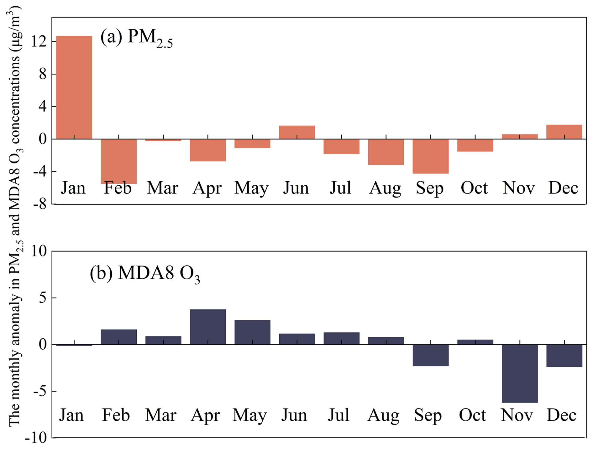
Figure 8 The monthly anomaly in PM_2.5 (a) and MDA8 O₃ concentrations (b) driven by the changing daily emissions for Jiangsu Province in 2022, based on the MLR model.

The anthropogenic-driven variability of PM_2.5 concentration was basically consistent with the temporal variation of estimated emissions. As shown in Fig. 8a, the abundant emissions in January resulted in a prominent enhancement of 12.7 µg m⁻³ for PM_2.5 concentration, followed by December (1.8 µg m⁻³) and June (1.6 µg m⁻³). In particular, the enhancement of June was driven largely by the post-pandemic economic recovery, as discussed in in Sect. 3.2. For most warm months (April–October, except June), negative impacts of anthropogenic activities on PM_2.5 level were found, ranging 1.1–4.2 µg m⁻³. Clear decline of PM_2.5 due to emission change was also found in February (5.5 µg m⁻³), resulting probably from the greatly reduced human activities (industry and transportation) during the Chinese New Year holiday. The PM_2.5 growth occurred during winter heating period highlighted the necessity of accelerating transition of clean household energy and improving management of industrial production after the short-term lockdowns.

The variation of anthropogenic emissions was found to elevate O₃ concentrations in most months of the year, particularly for warm seasons (Fig. 8b). The enhancements during March-August ranged 0.8–3.8 µg m⁻³, suggesting the important role of human activities in aggravating O₃ pollution. High temperature in summer promoted the emissions of temperature-dependent O₃ precursors, particularly NMVOCs from various sources (Fig. 2d). In addition, the NO_x emissions from certain sources were elevated in warm seasons, e.g., those from off-road machinery in the summer harvest season (Fig. 2a). The growing abundance of precursors, together with high temperature, enhanced the photochemical production rate of O₃.

However, the anthropogenic emissions during winter demonstrated a net negative contribution to surface O₃ concentrations (e.g., −6.2 and −2.4 µg m⁻³ for November and December, respectively), indicating a shift in the chemical regime of O₃ formation. Although the NO_x emissions were not enhanced in winter (Fig. 4), the weak photochemical production under low temperature and solar radiation made the NO_x titration more dominating in O₃ chemistry, primarily resulting in this net negative contribution. Simultaneously, reduced NMVOCs emissions and diminished photochemical activity restricted the efficiency of radical-driven O₃ production. The resulting O₃-depleting reactions overwhelmed potential formation mechanisms, leading to the estimated negative contribution from anthropogenic emissions. This pattern contrasted sharply with the net positive effect of anthropogenic activities in summer months, and underscored the complex season-dependent response of O₃ level to the changing precursor emissions.

3.4.2 Impact of fluctuations in anthropogenic emissions by precursor and sector on PM_2.5 and MDA8 O₃ concentrations

The impacts of anthropogenic emission fluctuations on variability of PM_2.5 and O₃ concentrations were quantified by precursor and sector, with a machine learning framework integrating XGBoost and SHAP analysis. Derived from the 10-fold cross validation, the correlation coefficient (R) between machine learning prediction and observation reached 0.78 and 0.81 for daily PM_2.5 and MDA8 O₃, respectively, suggested satisfying capability of the machine learning framework in predicting the anthropogenic-driven variability of PM_2.5 and O₃ concentrations (Fig. S12).

Figure 9a and b illustrates the contributions of changing emissions from different pollutant-sector combinations to the variability of PM_2.5 concentration in January and that of MDA8 O₃ in July, respectively. The temporal variability of PM_2.5 level attributable to anthropogenic emission changes was in general consistent with that of observed surface PM_2.5 concentration (Fig. 9a). For O₃, there existed some discrepancy between the temporal distribution of anthropogenic-driven variability and observed concentration in summer. This discrepancy may be attributed to the substantial impacts of meteorological conditions and biogenic VOCs emissions on O₃ formation (Gu et al., 2023).

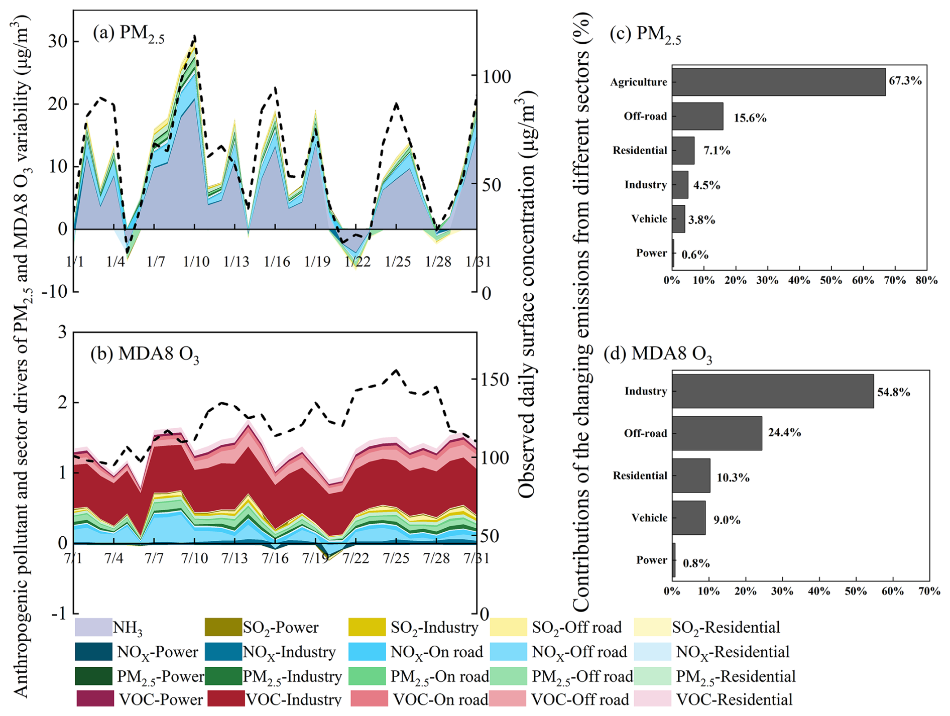
Figure 9 Anthropogenic pollutant and sector drivers of PM_2.5 and MDA8 O₃ variability. Panels (a) and (b) illustrate the contributions of pollutant-sector combinations to the variability of PM_2.5 in January and that of O₃ in July, derived from SHAP analysis. The black dashed lines represent the observed daily ground-level concentrations of PM_2.5 and MDA8 O₃. Panels (c) and (d) provided the contributions of the changing emissions from different sectors, with those of various precursor species aggregated.

Among all the pollutant-sector combinations, fluctuations in agricultural NH₃ emissions accounted for 67.3 % of the variability of PM_2.5 concentrations in January, followed by off-road NO_x (12.9 %) and residential PM_2.5 emissions (4.9 %). The contribution of NH₃ emission variation significantly exceeded those of NO_x (17.7 %), PM_2.5 (10.8 %), and SO₂ (4.2 %), suggesting that Jiangsu may be transitioning to an NH₃-rich regime following substantial reductions in SO₂ and NO_x emissions (Zhao et al., 2020b). Therefore, agricultural NH₃ control has become the priority of the strategy design for PM_2.5 pollution alleviations, compared to traditional NO_x abatement. The fluctuations in VOC-Industry contributed to 48.5 % of the variability of MDA8 O₃ concentrations in July, followed by off-road VOCs (9.7 %) and NO_x emissions (8.9 %). In total, the NMVOCs accounted for 69.7 % of the anthropogenic-driven variability of O₃ concentration, exceeding the contributions from NO_x (14.5 %), PM_2.5 (11.0 %), and SO₂ (4.9 %). The positive contribution of NO_x to MDA8 O3 indicated that the O₃ formation mechanism in Jiangsu may be shifting from a VOCs-limited regime towards a transitional or NO_x-limited regime. Regarding the sector contributions with various species aggregated, the agricultural emission fluctuations contributed most to anthropogenic-driven variability of PM_2.5 concentration (67.3 %, Fig. 9c), while industrial activities contributed most to that of O₃ concentration (54.8 %, Fig. 9d). Notably, off-road transportation emerged as an important contributor to both pollutants (15.6 % for PM_2.5 and 24.4 % for O₃), providing clear evidence for policy making of coordinating control of PM_2.5 and O₃ pollution.

4 Concluding remarks

In this study, we incorporated near-real-time activity data from multiple sources and developed a framework for continuously estimating the daily air pollutant emissions of anthropogenic origin. We then estimated the spatiotemporal evolution of emissions in Jiangsu Province, a typical developed area in eastern China, with a particular focus on the period during the COVID-19 lockdown in 2022 and the corresponding period after the lifting of restrictions in 2023. Finally, we constructed a rapid assessment approach that utilized machine learning algorithms to quantify the impact of fast changing emissions on variability of daily ambient concentrations of PM_2.5 and O₃.

We indicated that emission controls have played a crucial role in abatement of air pollutant emissions. The provincial emissions of SO₂, NO_x, PM_2.5, NMVOCs, and NH₃ decreased 17 %, 33 %, 18 %, 7 %, and 11 %, respectively, from 2019–2022. Implementation of ultra-low emission retrofits for industrial sectors has proven effective in reducing primary PM_2.5 and NO_x emissions. However, there is an urgent need to enhance NMVOCs emission control in key industrial sectors and areas. Regarding the temporal variabilities, the emissions of SO₂ and PM_2.5 were influenced greatly by fossil fuel consumption pattern, while NO_x emissions were increasingly dominated by that of transportation. The NMVOCs emissions peaked in the summer and declined in winter, followed by a rebound in emissions after the Chinese New Year. Comparative analysis showed that the emissions of NO_x, SO₂, PM_2.5, and NMVOCs in Jiangsu during the COVID-19 lockdown of Shanghai in April–May 2022 were respectively 8 %, 6 %, 6 %, and 10 % smaller than those in the same months of 2023. Transportation was identified as the primary contributors to the reductions in NO_x and PM_2.5 emissions, while industry accounted for 93 % of the reduction in NMVOCs, closely associated with the disrupted cross-regional product supply chains. Indicated by the contributions of changing emissions from pollutant-sector combinations to the variability of PM_2.5 and O₃ concentrations, reducing agricultural NH₃ emissions should be critical for PM_2.5 pollution alleviation, and off-road transportation has become a priority target for coordinating control of both PM_2.5 and O₃ pollution.

The near-real-time techniques and estimation of daily-level emissions offer substantial practical implications for current air quality management in China. Specifically, it can be directly integrated into the “Emergency Response for Reducing Heavy Pollution Weather” program. By providing the near-real-time feedback on emission variations, policy makers can reasonably determine the short-term emission reduction measures and timely evaluate their actual effectiveness (e.g., temporary suspension of specific industrial or traffic restrictions). Furthermore, combined with machine learning techniques, this framework allows policy makers to decouple the environmental benefits of long-term policies of air quality improvement from short-term emergency controls or unexpected socioeconomic shocks (like the COVID-19 lockdown). The obtained knowledge provides a scientific basis for formulating more cost-effective and reasonable strategies for coordinating the PM_2.5 and O₃ pollution controls.

Furthermore, the framework could be potentially applied for predicting future emission as it establishes a dynamic linkage between sector-specific activity factors and emissions. By adjusting these activity factors (such as the penetration of electric vehicles, the abatement of industrial production during haze events, and targeted reductions in agricultural activities), researchers and policy-makers could fast and reasonably project the emissions of diverse future scenarios. Coupled with the rapid assessment approach with machine learning, the framework presents a promising pathway to quantify how the emission changes might affect the daily variability of air quality, thereby better supporting the policy design and adjustment for regional complex pollution controls.

The limitations of this work exist mainly in the near-real-time information of multiple sources and the rapid assessment of air quality variability. For instance, CEMS were only applied for big point sources, thus we had to assume that the small and fugitive sources followed similar variability of emissions as point sources. As CEMS only covers SO₂, NO_x, and particles, the use of electricity consumption data for NMVOCs may introduce substantial uncertainty. Future improvement in online monitoring of NMVOCs will enhance the estimation of temporal variation of emissions. While our research framework demonstrates robust performance in Jiangsu Province, its heavy reliance on CEMS and provincial traffic monitors poses a limitation for its transferability to less developed regions or other developing countries without sufficient data support. To adapt this methodology for those regions, future applications could be expanded to other datasets with global accessibility. For instance, satellite-derived tropospheric NO₂ columns, daily nighttime light fluctuations, and generalized mobile phone signaling data could serve as alternative proxies to estimate the activity levels and their temporal profiles. Expanding this framework to incorporate such multi-source remote sensing data will be more crucial for establishing near-real-time emission inventories in regions with less data support. Moreover, the machine learning process ignored the contributions from regional transport, which could result in some bias in analyzing the impacts of anthropogenic emissions on air quality. However, in contrast to time-consuming numerical modeling, machine learning offered a rapid and reliable assessment of the impact of daily emission changes on air quality, and was thus recommended in future policy making of air pollution controls.