Top-down benchmark of US methane inventories reveals regional discrepancies in activity-based estimates

Robust estimates of methane emissions are critical for understanding their impacts on atmospheric warming and air quality, and for assessing methane mitigation strategies. Gridded inventories, such as the U.S. Environmental Protection Agency's Greenhouse Gas Inventory (EPA GHGI), the Emissions Database for Global Atmospheric Research (EDGAR 2024), and the National Oceanic and Atmospheric Administration's Fossil Fuel Oil and Gas inventory (NOAA FOG), are constructed to evaluate large-scale emission patterns and support identifying emission mitigation priorities and prioritizing future measurements. However, substantial differences across inventories complicate such assessments. We benchmark EPA GHGI, EDGAR 2024, and NOAA FOG against flux estimates from an atmospheric inversion of Greenhouse Gases Observing Satellite (GOSAT) data from 2012 to 2020 over the Contiguous United States (CONUS). A key technical challenge is the heterogeneous sensitivity of satellite-derived fluxes, which depends on measurement uncertainty, coverage, and inversion model configuration. We account for this heterogeneity by applying an inversion operator to each inventory prior to comparison with the GOSAT-based estimates. The GOSAT estimates are most sensitive to oil and gas and livestock emissions; oil and gas emissions are consistent with NOAA FOG (14.1 Tg CH₄ yr¹ in 2015), but exceed EPA GHGI and EDGAR, particularly across Texas, Oklahoma, and Louisiana. GOSAT-based livestock emissions exceed EPA GHGI and EDGAR by 1–2 Tg CH₄ yr¹, with the largest differences in the Midwest and California. Despite these discrepancies, both activity and satellite based estimates show no observable trends from 2012 to 2020 in fossil and livestock emissions.

1 Introduction

All GOSAT-derived emissions and corresponding inputs/algorithms are available at https://doi.org/10.5281/zenodo.15786798 (Worden and Pandey, 2025).

Jupyter/python code at https://doi.org/10.5281/zenodo.16921536 (Pandey and Worden, 2025) shows how to compare these GOSAT derived emissions to inventories.

Methane is a potent greenhouse gas that plays a significant role in atmospheric warming (Saunois et al., 2020). Methane is emitted from multiple anthropogenic sources including livestock, oil and gas exploitation, manure, rice cultivation, wastewater, solid waste, and coal mining, and from natural sources, particularly wetlands. Methane is also the main component of natural gas, a valuable global commodity that can pose safety risks when it leaks. Accurate and verifiable estimates of its emissions are essential for tracking progress and guiding effective mitigation strategies, and for accounting for the economic value of energy waste (IEA, 2025; World Bank, 2025). Gridded methane emission inventories, such as the gridded United States Environmental Protection Agency's Greenhouse Gas Inventory (EPA GHGI), the Emissions Database for Global Atmospheric Research 2024 release (EDGAR 2024), and the National Oceanic and Atmospheric Administration's Fuel-based Oil and Gas inventory (NOAA FOG), are widely used for comparing sectoral emissions, primarily at the regional scale, to atmospheric data (EPA, 2023; Maasakkers et al., 2023; Crippa et al., 2020, 2024a, b; Francoeur et al., 2021; Kruskamp et al., 2025). However, discrepancies in how the inventories are generated, e.g. from emission factor assumptions, activity data, and/or spatial proxies and resolution can result in substantial variation in both the magnitude and sectoral attribution of emissions (Hristov et al., 2017; Alvarez et al., 2018; Maasakkers et al., 2021; Petrescu et al., 2024; Gordon 2025). In some cases, differences between inventories can be as large as the emissions themselves (Fig. 1), complicating the evaluation of national and regional emission trends. Verification of their underlying parameterizations is often limited by spatiotemporal mismatches between empirical measurements and inventory assumptions. Moreover, differences between activity-based emissions and flux estimates based on observations combined with atmospheric modeling (e.g., top-down atmospheric inversions) can far exceed the changes inferred from the observed growth in atmospheric methane concentrations (Nisbet et al., 2019; Worden et al., 2022). As a result, tracking mitigation progress using bottom-up inventories alone could be unreliable without independent observational constraints. In addition to these uncertainties, emissions missing in the inventories pose another significant challenge. For instance, sporadic high emitters in both fossil fuel production and waste management, often caused by mechanical failures, may not be captured in traditional inventories (Cusworth et al., 2020; 2024; Sherwin et al., 2024); consequently, the magnitude of these emissions remains poorly understood.

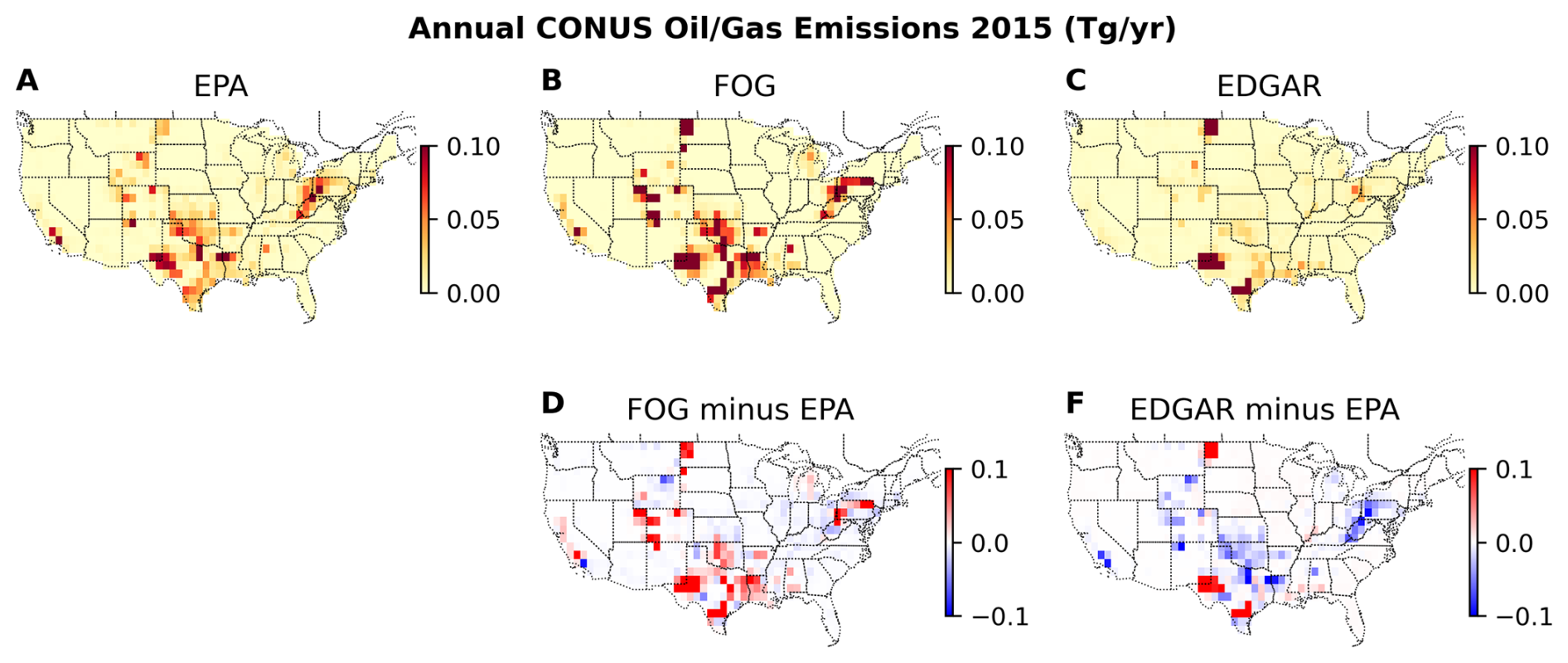
Figure 1 (Top Panels) Mean Emissions for Oil and Gas for 2015 (at 1° × 1° long/lat gridding) as calculated from the EPA, FOG, EDGAR inventories. (Bottom Panels) Differences between FOG and EPA and EDGAR and EPA.

To evaluate potential uncertainties in bottom-up inventories, top-down emissions estimates derived from satellite observations, such as those from the Greenhouse Gases Observing Satellite (GOSAT), provide a valuable, independent constraint. These atmospheric measurements inherently capture all emissions influencing methane concentrations, including unreported or underestimated sources, and therefore offer a more comprehensive view of total methane emissions. However, the resulting estimates and their information content (spatial resolution + uncertainties) depend strongly on the observational sampling, sensitivity of the observation to the emissions, choice of a priori fluxes, and the inversion regularization. Consequently, over regions with limited sampling, e.g., due to clouds or low sunlight, top-down analyses have greatly reduced sensitivity to nearby emissions, so the estimates there simply reflect the a priori. In contrast, emissions inferred for regions with ample sampling are more likely to accurately represent local sources. The focus of this paper is to demonstrate how this GOSAT-based benchmark can be used to evaluate alternative gridded inventories while accounting for its variable information content as discussed next.

2 Integrated total and sectoral USA emissions for 2015

Table 1 summarizes US methane emissions by sector for 2015, based on the GOSAT data and the sectoral attribution approach described in this study (Appendix A). The error characterization (Appendix B) includes uncertainties from the a priori as well as measurement and model systematic error. The prior emissions are taken from Worden et al. (2023). Table 1 also shows a quantity called the Degrees of Freedom for Signal (DOFS), which is given by the trace of the averaging-kernel matrix for the corresponding state-vector elements in z. The DOFS describe the extent to which the estimate is informed by observations rather than prior assumptions (Appendix B), as well as the spatial information content. For example, from Eq. (2), if A≈0 (equivalent to DOFS = 0), observations say essentially nothing about the emissions and the estimate reduces to the prior. If A is the identity matrix, then the DOFS equals the number of state-vector elements and the estimate exactly reflects the true distribution, modified by the expected uncertainties (Appendix B). The DOFS reported in Table 1 refer to the spatially distributed estimate, not for the total emissions value. Hence, DOFS > 1 means there is at least some spatial information for that sector's estimate.

Table 1 GOSAT-Based CONUS Anthropogenic Emissions and Information Content by Sector (2015).

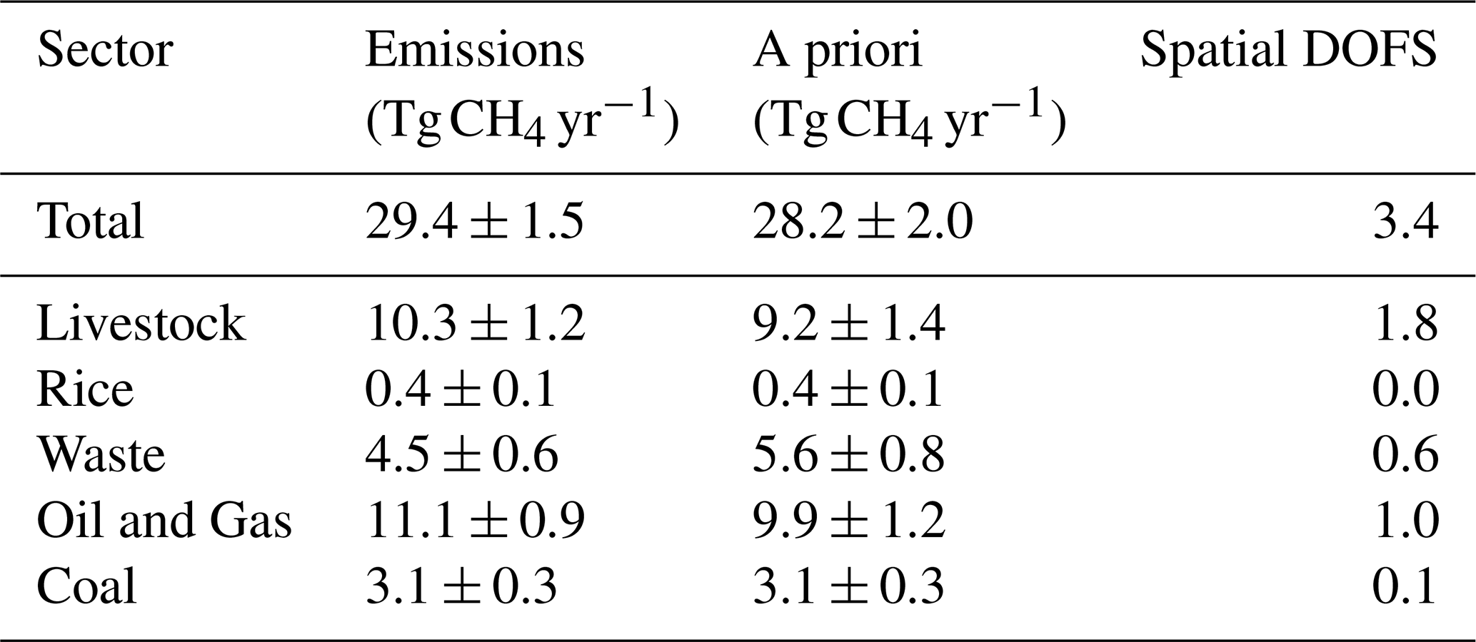
For this GOSAT-based benchmark, the highest information content is available for total, livestock, and oil and gas (O&G) emissions, while waste emissions estimates are only moderately constrained by the data, and rice and coal emissions have limited observational information. This variability in information content underscores the need for careful interpretation of top-down estimates, particularly when examining spatial and sectoral patterns or trends.

Table 2 Comparison of Methane Emissions by Study. All totals are CONUS anthropogenic emissions for the years listed. Atmospheric inversions exclude natural sources and fire emissions where sectoral separation is available. Activity-based estimates include the gridded EPA GHGI, EDGAR 2024, and NOAA FOG inventories evaluated in this study.

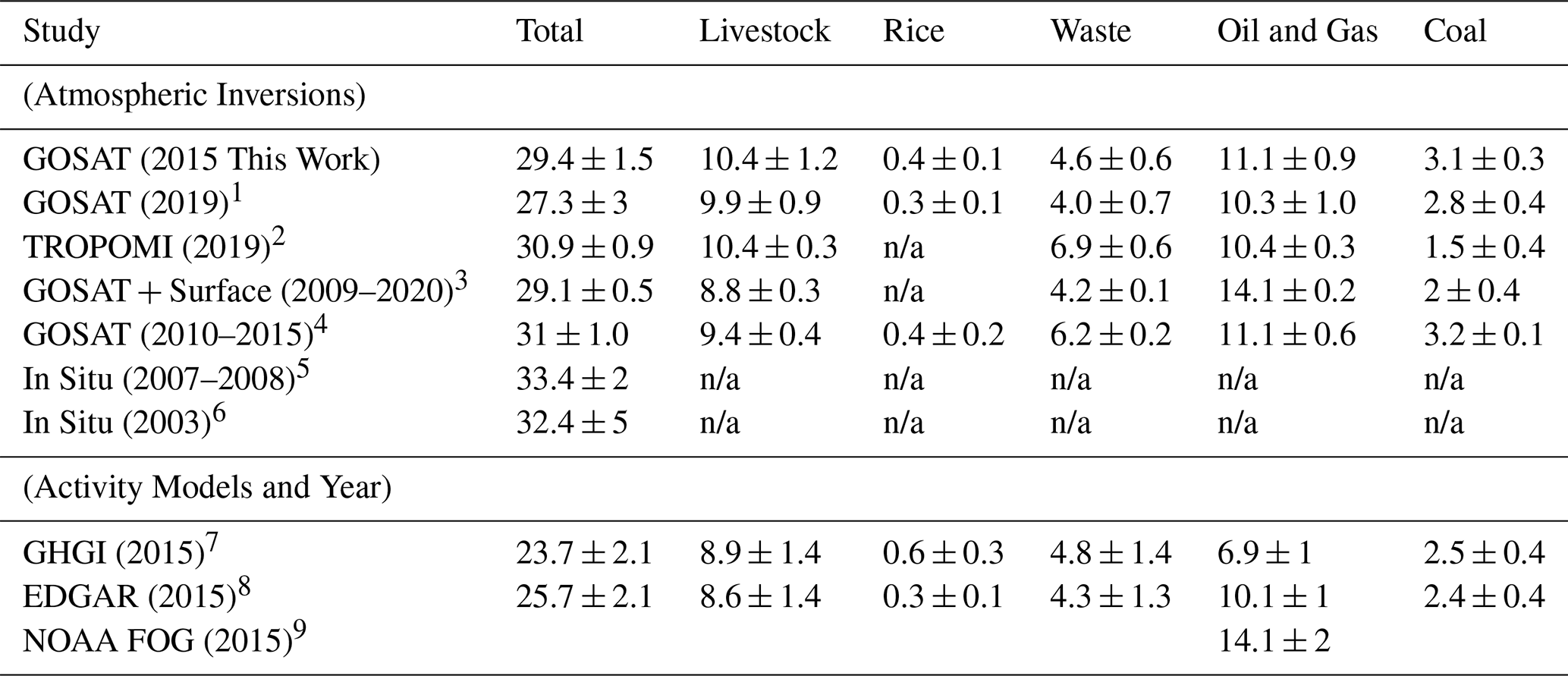
References: ¹ Worden et al. (2022), ² Nesser et al. (2024), ³ Janardanan et al. (2024), ⁴ Maasakkers et al. (2019), ⁵ Miller et al. (2013), ⁶ Kort et al. (2008), ⁷ Maasakkers et al. (2016, 2023), ⁸ Crippa et al. (2024a, b), and ⁹ Francoeur et al. (2021). n/a: not applicable

Table 2 compares our emissions to previous inversions using atmospheric data and to the inventories discussed in this paper (Appendix C). As can be seen in Table 2, our atmospheric-based emissions are generally consistent with other studies, typically within 1–2 standard deviations of the reported uncertainties, even though each study uses different priors, has different systematic errors, and has different sensitivity to the underlying emissions. These comparisons also show that total emissions from atmospheric-based inversions are typically larger than activity-based estimates, with the livestock and oil and gas sectors responsible for most of the discrepancy.

2.1 Oil and Gas Emissions (GOSAT, FOG, EPA, and EDGAR)

We next compare the GOSAT-based emissions for O&G to those from NOAA FOG, GHGI, and EDGAR inventories. In particular, we demonstrate how applying the inversion operator to these inventories modifies our interpretation of the comparison.

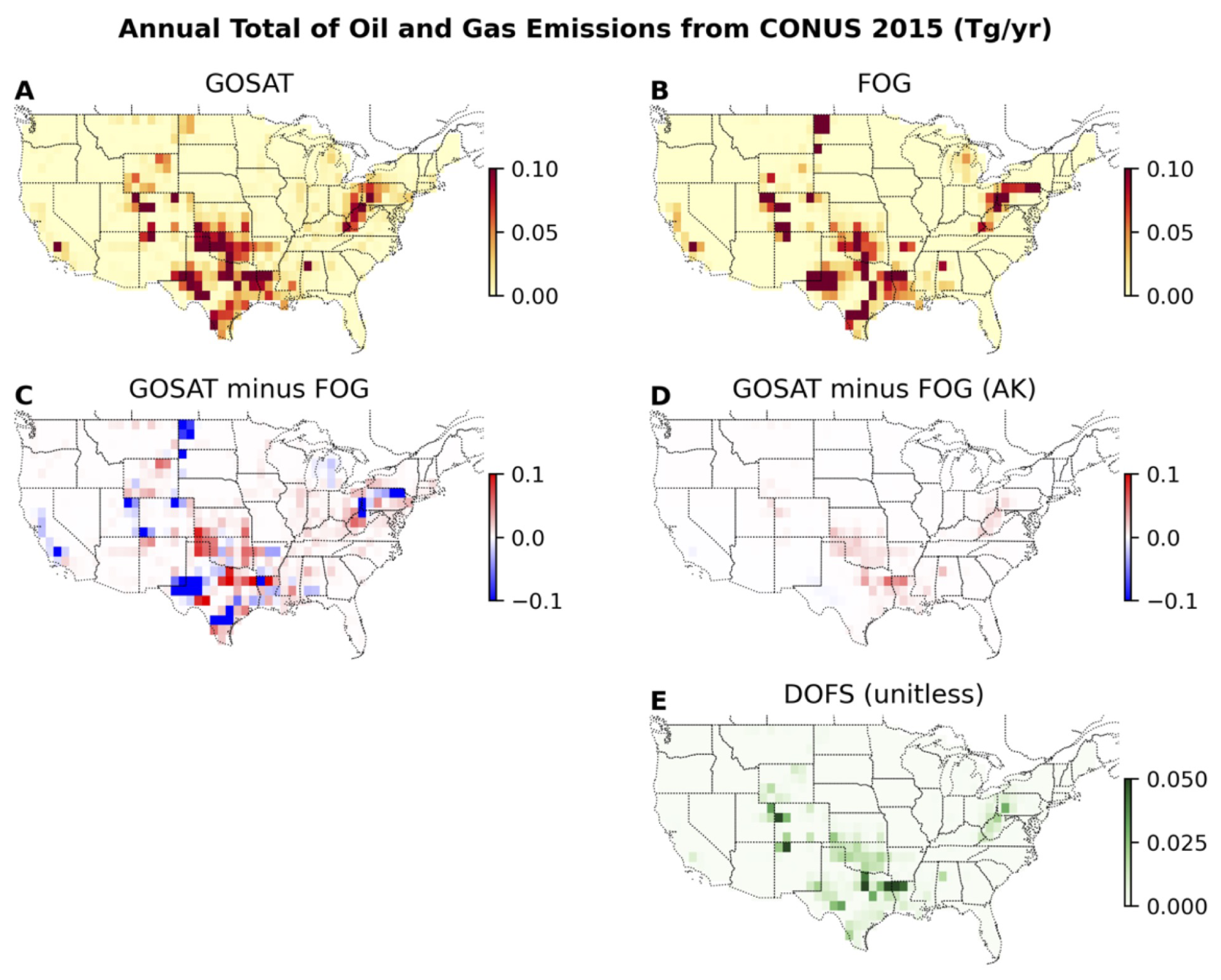
Figure 2 Comparison of the US oil and gas (O&G) methane emissions in 2015 from the GOSAT inversion with those from the FOG inventory. Panel (A) shows the GOSAT based estimate. Panel (B) shows the original FOG emissions. Panel (C) shows the difference between the top two. Panel (D) shows the difference between FOG emissions and GOSAT based emissions after applying the inversion operator (denoted AK). All figures use 1° × 1° gridding; only differences larger than the corresponding calculated uncertainty are shown. Panel (E) shows the diagonal of the averaging kernel (or DOFS) corresponding to that location for oil and gas emissions.

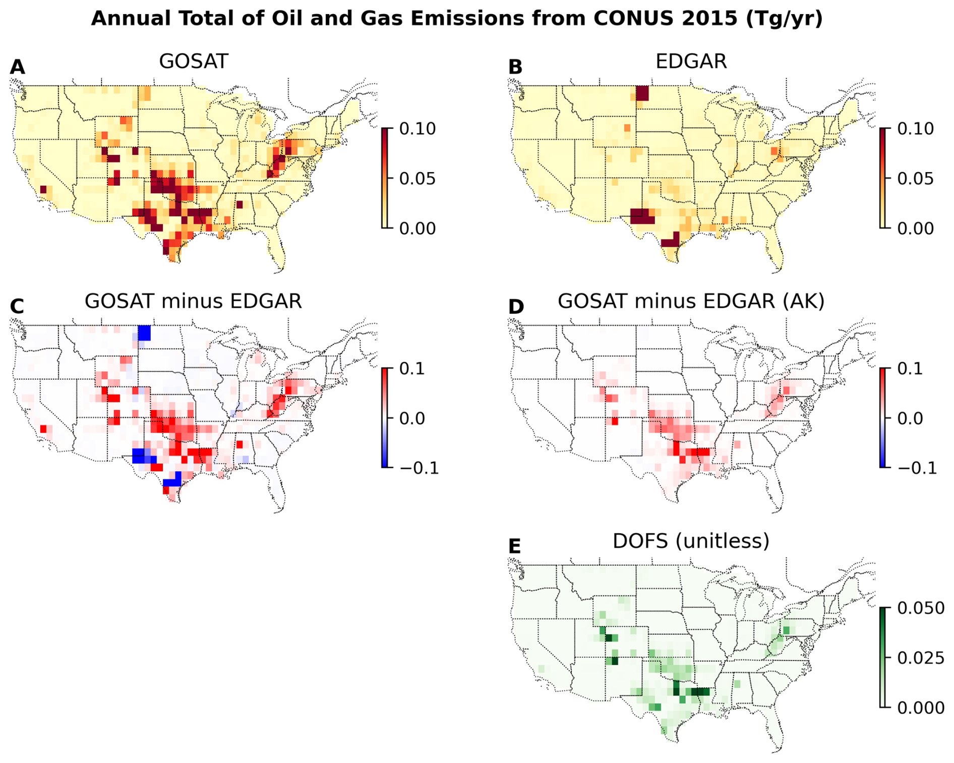
Figure 3 Same as in Fig. 2 but for the EDGAR inventory.

Spatial Distribution for 2015. Figures 2 through 4 compare the spatial distribution of US oil and gas (O&G) methane emissions in 2015 from the GOSAT inversion with those from the FOG, GHGI, and EDGAR (2024 release, Crippa et al., 2024a, b) inventories, respectively. These comparisons demonstrate the importance of accounting for the varying information content of the GOSAT inversion, which is influenced by both the prior emissions used in the inversion and the sensitivity of the aggregated satellite observations to underlying emission patterns (Worden et al., 2023 and references therein). In Fig. 2, the upper left panel (Fig. 2A) shows the GOSAT based estimate. The upper right panel (Fig. 2B) shows the original FOG emissions. The middle left panel (Fig. 2C) shows the difference between the top two. The middle right panel (Fig. 2D) shows the difference between FOG emissions and GOSAT based emissions after applying the inversion operator (denoted AK). All figures use 1° × 1° gridding. The bottom right panel (Fig. 2E) shows the diagonal of the averaging kernel (or DOFS) corresponding to that location for oil and gas emissions. As seen in the left panel of Fig. 2, significant regional discrepancies between the GOSAT and FOG inventories exist, with similar magnitude differences as shown in Fig. 1. However, after applying the inversion operator (Eq. 2) to the FOG inventory (labeled FOG AK), many of these differences are greatly reduced (middle right panel)

Small differences between GOSAT and the inventory, after applying the inversion operator, can also occur because of limited sensitivity, as indicated by the DOFS, for example over the Bakken region of North Dakota. As discussed previously and shown in Eq. (2) and Appendix B, in such cases the difference between the GOSAT estimate and the inventory adjusted by the inversion operator should be close to zero, because both terms reduce to ∼ z_A. In contrast, the GOSAT estimate shows increased sensitivity to emissions in Oklahoma, Texas, and Louisiana. Based on this comparison, and on the integrated total emissions in the next section, we conclude that the GOSAT estimate does not falsify the spatial distribution of methane emissions posited by the FOG oil and gas inventory.

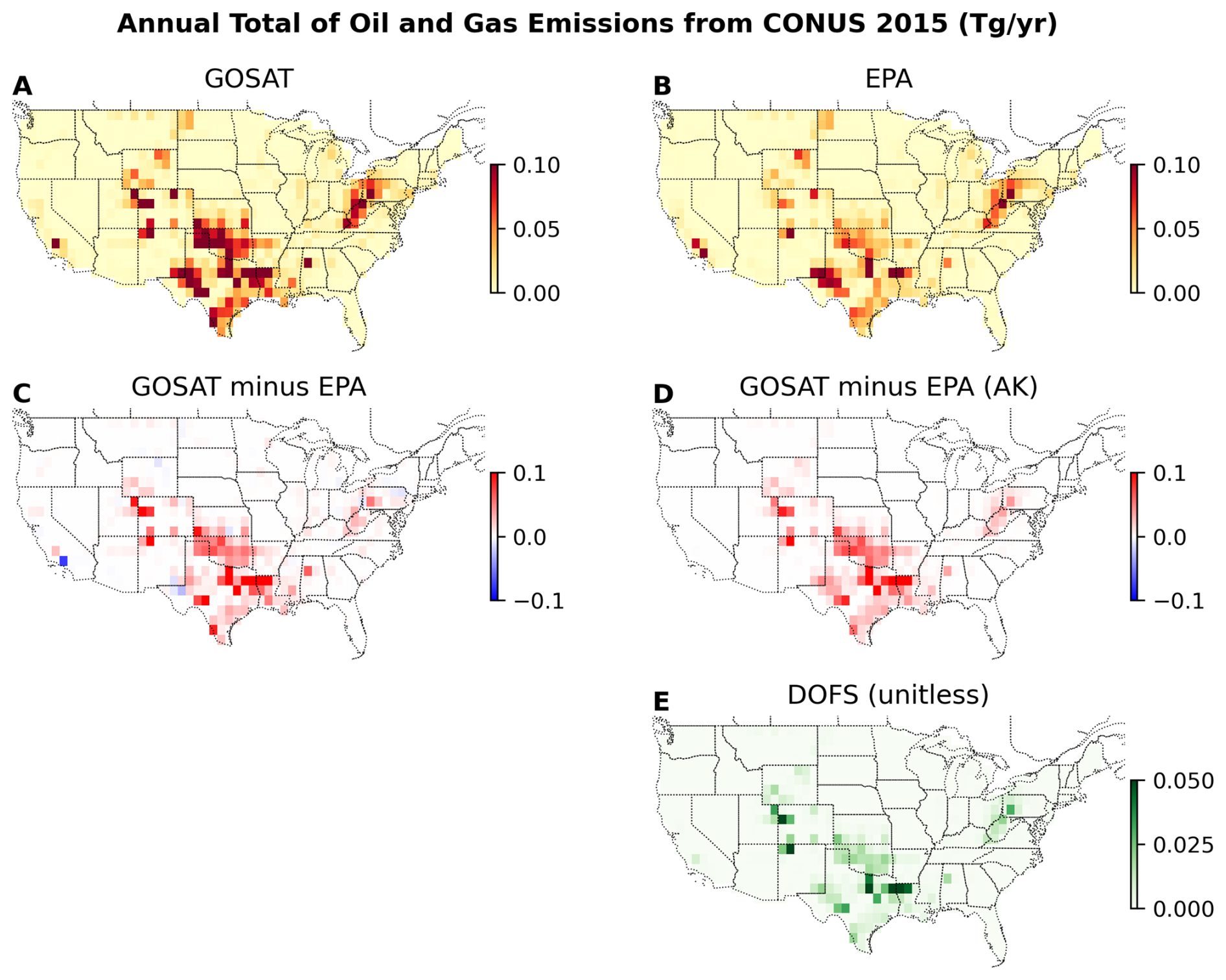
Figure 4 Same as in Fig. 3 but for the EPA GHGI inventory.

Interpreting Comparisons between GOSAT, EDGAR, and GHGI emissions. Comparisons between GOSAT and EDGAR (Fig. 3) and between GOSAT and EPA GHGI (Fig. 4) show larger discrepancies, even after applying the inversion operator, particularly in northwest Colorado, Texas, Oklahoma, and Louisiana. These patterns indicate substantial inventory uncertainties in well-observed regions with intensive oil and gas activity. Some regions are sparsely observed by GOSAT, so their contributions may be important but their uncertainties cannot be reliably assessed with this benchmark. When measurement cost is a constraint, the discrepancy hotspots identified here are high-value targets for additional observations, with expanded coverage of under-sampled regions as resources allow.

Previous studies (e.g., Alvarez et al., 2018; Cusworth et al., 2022; Sherwin et al., 2024) have shown that a small number of high emitters (e.g., < 2 %; Sherwin et al., 2024), likely due to unplanned mechanical failures, contribute disproportionately to the fossil methane budget. These sources are likely underrepresented or missing from activity-based inventories. The agreement between FOG and GOSAT supports this conclusion, as the FOG inventory integrates atmospheric CH₄ with NO_x observations and activity metrics; these regional CH₄ observations capture emissions under-represented in purely bottom-up approaches. If such super-emitters are entirely responsible for the discrepancies between GOSAT and the EPA GHGI and EDGAR inventories, then comparisons between the GOSAT, EPA, EDGAR, and FOG O&G emissions in Table 2 suggest these sources are undercounted by ∼ 7 Tg CH₄ yr⁻¹ of reported natural gas emissions, far exceeding previous estimates, as previously documented in other studies (e.g., Alvarez et al., 2018; Cusworth et al., 2022; Sherwin et al., 2024; Zavala-Araiza et al., 2015).

Integrated totals for 2015. Figure 5 compares integrated total oil and gas (O&G) emissions derived from GOSAT with those from the FOG, GHGI, and EDGAR inventories.

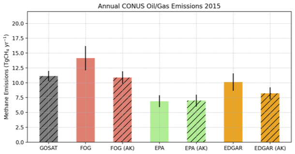
Figure 5 Comparison of the integrated total oil and gas (O&G) emissions derived from GOSAT with those from the FOG, EPA GHGI, and EDGAR 2024 inventories, both with and without the inversion operator (AK) applied. Comparisons should be made between the GOSAT estimate and the inventories with inversion operator (AK) applied.

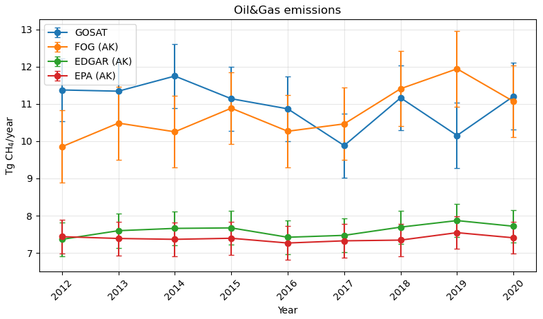
Figure 6 Integrated totals for oil and gas emissions between 2012 and 2020. The GOSAT inversion operator has been applied to the FOG, EPA GHGI, and EDGAR 2024 inventories; the biases between the comparisons are therefore not due to the prior used with the GOSAT inversion.

Before applying the inversion operator, total FOG emissions are estimated at 14.1 ± 2 Tg CH₄ yr¹. We assumed the same prior covariance structure (Z_A, Appendix B; Worden et al., 2022, 2023) for FOG as for the GOSAT a priori. This yields a smaller total uncertainty (2 Tg CH₄ yr¹) than the ∼ 2.8 Tg CH₄ yr¹ uncertainty for total FOG O&G emissions inferred from a Monte Carlo analysis of NO? activity data (Francoeur et al., 2021). Using a different covariance structure that is consistent with the stated uncertainty in total emissions could therefore change conclusions about whether the GOSAT estimate falsifies the FOG inventory, and the inversion-operator methodology in Eq. (2) would allow this. However, a full covariance is required, with explicitly computed off-diagonal terms such that, when projected to a single number, it reproduces the expected uncertainty reported in, for example, Francoeur et al. (2021).

After applying the inversion operator, the FOG total is reduced to 11.4 Tg CH₄ yr¹. The uncertainty shown for the modified FOG estimate (denoted FOG-AK) reflects the uncertainty in the difference between the GOSAT-based estimate and the FOG-AK estimate (Appendix B, Eq. B4), not the uncertainty of the FOG-AK estimate itself. Because the FOG-AK estimate is consistent with the GOSAT-based inversion within the reported uncertainty, this comparison suggests that the GOSAT estimate does not falsify the original, higher FOG total of 14.1 Tg CH₄ yr¹.

Figure 5 also shows comparisons to GHGI and EDGAR. For these inventories, uncertainties prior to applying the inversion operator are derived using the same prior covariance structure as for the GOSAT a priori, because published full covariances are not readily available.

In contrast to the FOG comparison, both the EPA and EDGAR estimates, with or without application of the inversion operator, are inconsistent with the GOSAT-based inversion. Their differences lie well outside the post-operator uncertainty shown for each inventory. As shown in Figs. 3 and 4 these differences are spatially located primarily in the Texas, Oklahoma, and Louisiana regions. As noted previously, additional measurements here are therefore likely to reduce uncertainties in the USA O&G methane budget.

Integrated Totals: 2012–2020. Figure 6 shows annual methane emissions from 2012 to 2020. Despite substantial increases in oil and gas production over this period, all gridded inventories and the GOSAT top-down estimates show no significant change in total US methane emissions, although the FOG inventory may have a slight increase. This apparent disconnect between rising production and stable emissions has been noted in several studies and is commonly attributed to improvements in production efficiency, leak detection, and emissions control technologies (e.g., Lu et al., 2023). EPA GHGI supports this conclusion, showing relatively flat changes in fossil fuel methane emissions over the same period. This stability in the activity estimate is explained by offsetting trends, including a decline in exploration emissions due to fewer well completions, the adoption of lower-emitting equipment, and stable or slightly declining well counts (Maasakkers et al., 2023). For instance, while natural gas production increased by 26 % and crude oil production by 67 %, the number of active gas and oil wells remained roughly constant, declining slightly over the period. Emissions from gas systems were flat overall, with increases in gathering and boosting offset by decreases in production and processing. Similarly, petroleum system emissions rose by just 11 % due to a significant drop in exploration-related emissions (Maasakkers et al., 2023).

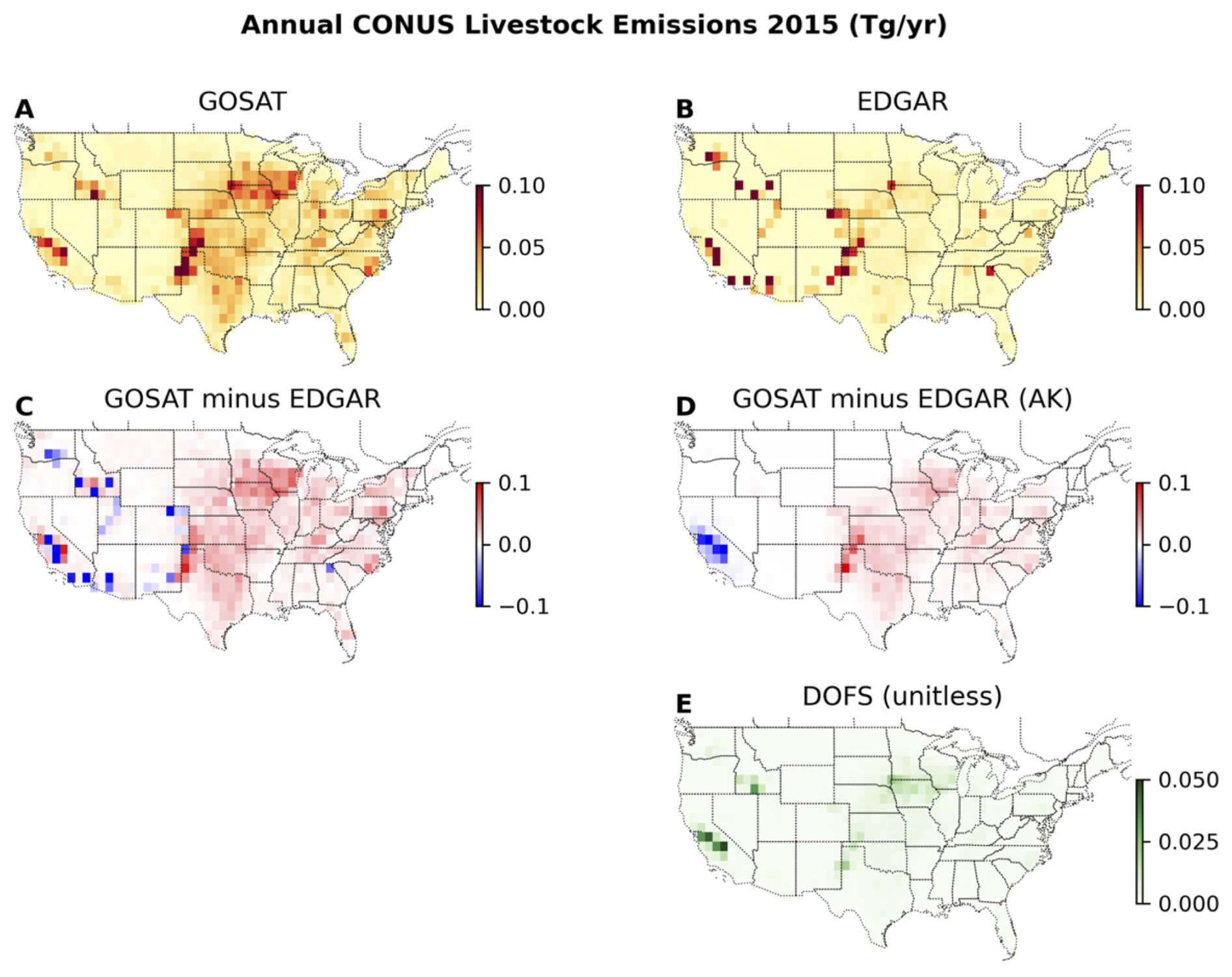
Figure 7 Similar to Fig. 2 but for EDGAR 2024 livestock emissions.

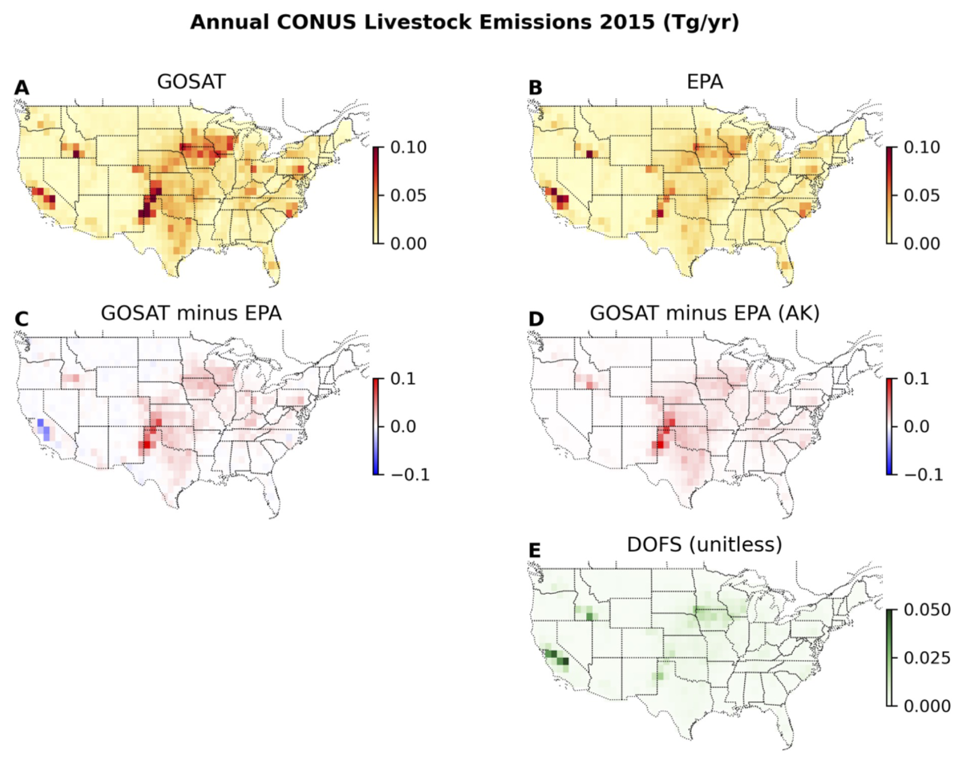
Figure 8 Similar to Fig. 7 but for EPA GHGI livestock emissions.

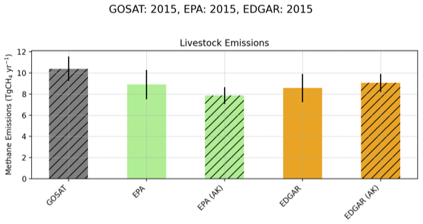
Figure 9 Comparison of the integrated livestock emissions derived from GOSAT with those from the EPA GHGI and EDGAR 2024 inventories, both with and without the inversion operator (AK) applied. Comparisons should be made between the GOSAT estimate and the inventories with inversion operator (AK) applied.

2.2 Livestock Emissions (GHGI and EDGAR)

Spatial Distribution for 2015: Similar to Figs. 2–4, Figs. 7 and 8 show the spatial distribution of livestock methane emissions from GOSAT, EDGAR, and GHGI data. The FOG inventory is limited to oil and gas emissions and is therefore excluded from this and subsequent comparisons. Methane emissions from livestock generally scale with herd size, particularly dairy and beef cattle. Dairy cows typically emit more than twice as much methane as beef cows, due to higher enteric fermentation (Wolf et al., 2017; Hristov et al., 2017). Emissions vary geographically with management and environmental conditions (for example grazing practices, feed quality, and temperature, Wolf et al., 2017). Inventories account for this using region-specific emission factors, but if the factors used are not representative of actual local conditions, the resulting difference between the atmospheric based and activity based emissions should be spatially structured rather than random. Consistent with this, we observe systematic regional biases relative to the GOSAT-based estimates: inventories in California and the northern states are higher than GOSAT, whereas inventories in northern Texas are lower.

Integrated Total for 2015. Figure 9 compares integrated livestock methane emissions from GOSAT with GHGI and EDGAR inventories, each shown with and without the inversion operator applied. The GHGI and EDGAR totals differ modestly. The EPA total lies slightly outside the GOSAT uncertainty range, while the EDGAR total falls within it. However, agreement in totals does not imply agreement in spatial patterns. For EDGAR in particular, closer total agreement with GOSAT coincides with offsetting regional deviations, with positive differences in parts of the Midwest and negative differences in California. These cancellations reduce the apparent mismatch in the national total, which underscores the importance of evaluating spatial variability alongside integrated totals. Overall, comparisons of integrated totals and spatial patterns indicate substantial remaining uncertainty in livestock emissions. Additional measurements over California and the Midwest, especially in the Texas and Oklahoma region, would likely reduce this uncertainty.

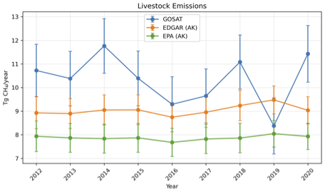
Figure 10 Integrated totals for Livestock Emissions between 2012 and 2020. The inversion operator has been applied to the inventories.

Integrated Totals for 2012–2020: Figure 10 (and Table 2) shows comparisons between the integrated total livestock emissions from the GOSAT based inversion and the GHGI and EDGAR inventories. The GOSAT-based estimate as well as those from the GHGI and EDGAR inventories do not observably change within the calculated uncertainties, except possibly for the year 2019. We therefore conclude that GOSAT based livestock emissions cannot falsify the posited (flat) trends from activity data (Maasakkers et al., 2021).

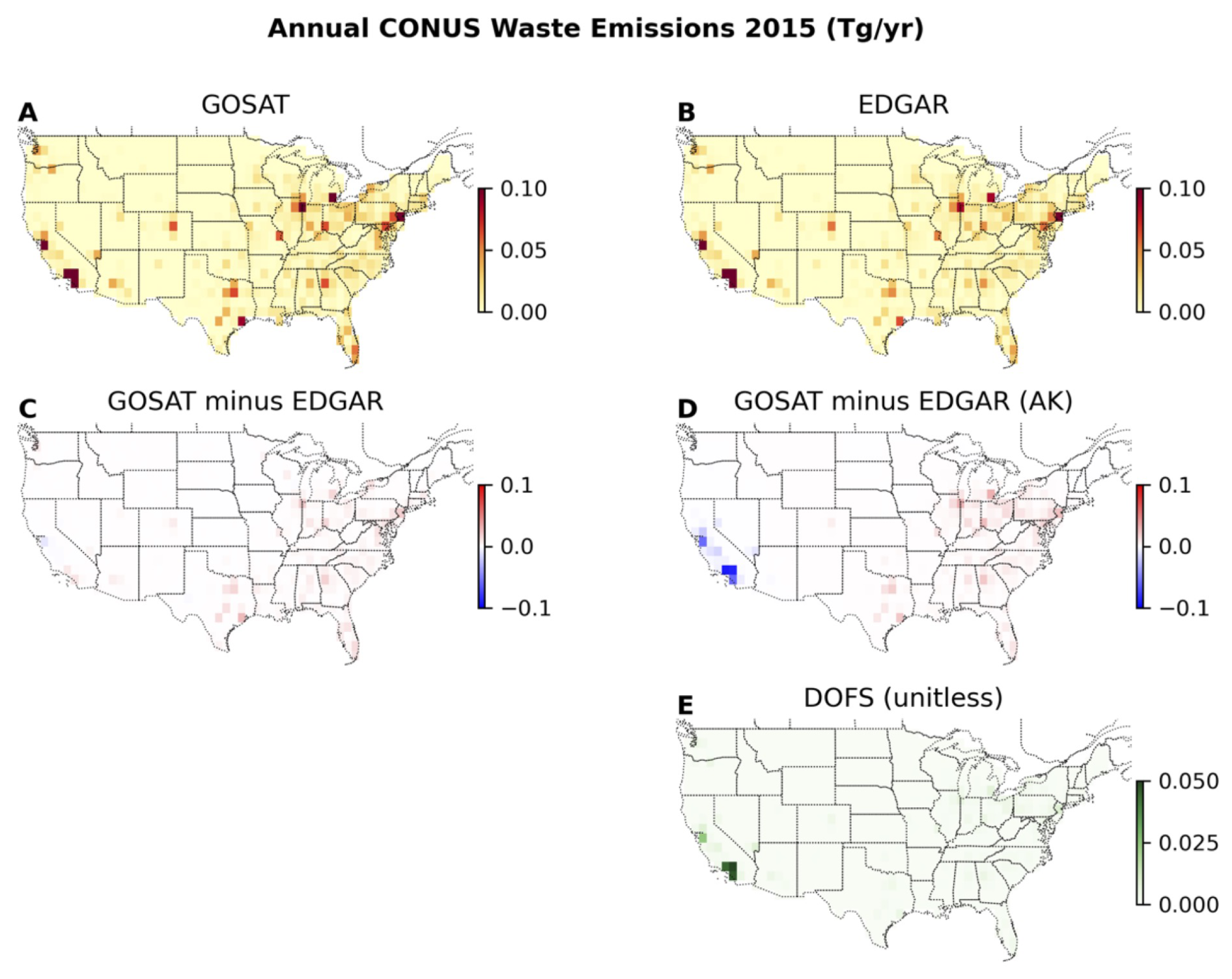
Figure 11 Similar to Fig. 2 but for EDGAR 2024 waste emissions.

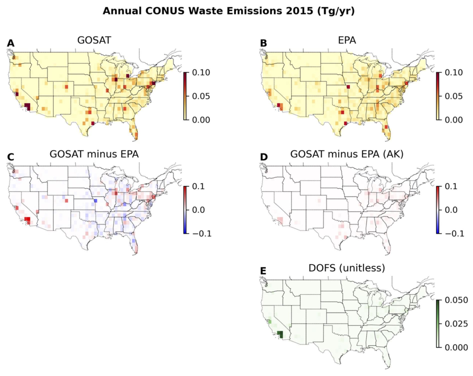
Figure 12 Similar to Fig. 3 but for EPA GHGI waste emissions.

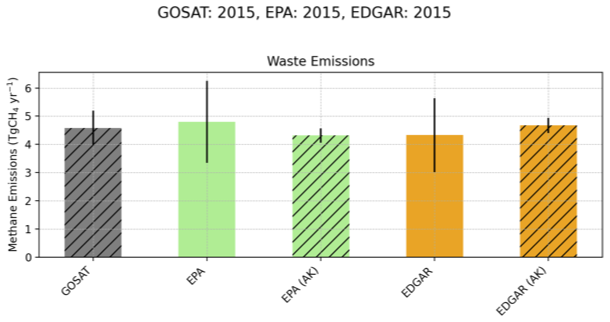
Figure 13 Integrated total methane emissions from the waste sector based on GOSAT, along with estimates from the EPA GHGI and EDGAR 2024 inventories, both with and without the inversion operator applied.

2.3 Waste (GHGI and EDGAR)

Figures 11 and 12 show the spatial distribution of methane emissions from the waste sector based on GOSAT, GHGI, and EDGAR estimates and Fig. 13 shows the integrated total for 2015. The largest differences are for California for the EDGAR$/$GOSAT comparison. The integrated waste sector methane emissions from GOSAT are estimated at 4.5 ± 0.6 Tg CH₄ yr⁻¹, while both GHGI and EDGAR report lower values of 4.2 ± 0.3 Tg CH₄ yr⁻¹. These differences are not statistically significant, as the GOSAT estimate lies within the uncertainty range of both inventories (after applying the inversion operator). However, there is very limited spatial information content in the GOSAT waste estimate (∼ 0.6 DOFS total). Consequently, the spatial differences shown in the right-bottom panel don't show meaningful differences between the inventories and the GOSAT waste estimate for most of the country. Because of this limited sensitivity we do not compare temporal changes in the waste emissions.

3 Summary and Future Directions

Top-down methane emissions estimates vary in their information content depending on the emission sector and observing system. For these GOSAT based emissions estimates, information content is greatest for oil and gas and livestock, so these sectors are best suited for inventory evaluation using the results shown here. Waste, coal, and rice exhibit lower information content in this analysis because GOSAT does not adequately sample methane variability attributable to those sources. Even so, our information-content-based comparison identifies where additional measurements would yield the largest uncertainty reductions in gridded inventories.

In particular, our results highlight the need for targeted measurement campaigns, especially in the Texas, Oklahoma, and Louisiana drilling basins, where additional data can most effectively reduce inventory uncertainties. For the livestock sector, California and Northern Texas stands out as key regions where improved activity based and atmospheric methane observation can have the highest impact. These findings underscore the importance of prioritizing high-emitting or uncertain regions to refine national methane budgets.

Beyond regional targeting, improving inversion resolution is also key. Higher-resolution flux estimates, whether through satellites like TROPOMI or plume-resolving instruments (e.g., Jacob et al., 2022; Pandey et al., 2025 and refs therein), are particularly needed for sectors such as waste, coal, and oil and gas, where coarse-resolution inversions struggle to isolate source signals. In particular, integrating plume-resolving and area-flux estimates enhances the sectoral attribution of emissions and improves the information content for inventory evaluation (Pandey et al., 2025).

(Trends) Inversions conducted using GOSAT data and GEOS-Chem (see references in Table 2), show no discernible trend over the analysis period, which is consistent with all three gridded inventories discussed in this manuscript. However, the fact that other inversions show different trends highlights the importance of benchmarking approaches (Janardanan et al., 2024), not only for validating inventories but also for identifying uncertainties in inversion outputs themselves. These differences matter for informing effective remediation strategies and setting realistic expectations for emission reductions.

As satellite constellations improve in spatial resolution, sampling, and accuracy, top-down flux estimates become more accurate at higher spatial resolution (e.g., Jacob et al., 2022). Using TROPOMI, Nesser et al. (2024) produced a 2019 North American emissions map with a degree of freedom for signal (DOFS) of ∼ 772, more than two orders of magnitude higher than in our GOSAT record, driven by a similar increase in observations. This resolution enables explicit estimation of many large sources, including landfills. East et al. (2025) extended this approach to global coverage at similar ∼ 25 km gridding. Building a benchmark from the combined record will help evaluate how countries have managed emissions before and after the Global Methane Pledge, which targets a 30 % reduction from 2020 to 2030. Our approach shows how inventories can be benchmarked against these improved flux estimates to reduce uncertainty, especially smoothing error, without re-running inversions with inventory priors. Combining high-resolution, independent datasets will support more accurate methane inventories, clarify source trends, and inform effective mitigation strategies.

Appendix A: GOSAT Methane Fluxes and Projection to USA Emissions by Sector

(Overview) Yearly sectoral emissions by region based on the satellite data are generated in a two step process. The first step is to quantify global integrated fluxes using total atmospheric column methane data from the Japanese GOSAT (Greenhouse gases Observing SATtellite) instrument (Parker et al., 2011) and the GEOS-Chem model (Zhang et al., 2021). The approach used to generate fluxes has been extensively documented in past literature (e.g. Zhang et al., 2021; Qu et al., 2024), and we refer the reader to these articles. The state vector for this inversion include (1) yearly anthropogenic methane emissions between 2010 and 2022 at a gridding of 5° × 4°s (longitude/latitude) and we use the estimates between 2012 and 2020 for this study, (2) wetland methane emissions for specified regions for each month between 2010 to 2022), and (3) the yearly hemispheric methane sink. The second step (next section) is a linear estimate based on an optimal estimation sectoral emissions attribution approach (Cusworth et al., 2021; Worden et al., 2022) that projects the integrated anthropogenic fluxes to emissions by sector and trends at the same 5° × 4° gridding and then again at 1° × 1° (long/lat) gridding over the USA. This projection accounts for the prior distribution and uncertainties in the emissions (e.g. Worden et al., 2022). We next provide more detail on projection/attribution methodology as it is relevant to the benchmarking methodology that is the focus of this paper.

(Sectoral attribution of fluxes to emissions) We use a Bayesian based approach to project the fluxes described in the previous section (at 5° × 4° long/lat) to emissions by sector at 1° × 1°. The full methodology is described in Cusworth et al. (2021) and first applied to methane fluxes in Worden et al. (2022) and again in Worden et al. (2023). This approach is equivalent to swapping the a priori assumptions, given by x_A and S_A, to a different state vector z_A (and a priori covariance Z_A) when a linear relationship between the different state vectors x and z exist. The approach provides the full posterior and prior covariances and priors needed to account for the varying information content of satellite based emissions estimates when comparing these emissions to either each other (e.g. between years) or to inventories (Worden et al., 2023) or to other estimates. We refer the reader to these papers, starting with Cusworth et al. (2021) for the primary derivation, and summarize here.

Given a linear mapping between one state vector and another (e.g. between fluxes x at 5° × 4° versus emissions z at 5° × 4° or alternatively emissions at 1° × 1°):

$$\begin{array}{}\text{(A1)}& \mathit{x}=\mathbf{M}\mathit{z}\end{array}$$

As discussed in Worden et al. (2023), the solution for projecting fluxes back to emissions takes the form:

$$\begin{array}{}\text{(A2)}& \begin{array}{rl}\widehat{\mathit{z}}=& {\mathit{z}}_{\mathrm{A}}+\widehat{\mathbf{Z}}{\mathbf{M}}^{\mathrm{T}}{\widehat{\mathbf{S}}}^{-\mathrm{1}}\\ & \times \left[\left(\mathbf{I}-\widehat{\mathbf{S}}{\mathbf{S}}_{\mathrm{A}}^{-\mathrm{1}}\right)({\mathit{x}}_{\mathrm{A}}-\mathbf{M}{\mathit{z}}_{\mathrm{A}})+(\widehat{\mathit{x}}-{\mathit{x}}_{\mathrm{A}})\right]\end{array}\end{array}$$

where the $\widehat{\mathit{z}}$ and z_A is the posterior and prior emissions state vector, respectively with posterior and prior error covariance $\widehat{\mathbf{Z}}$, Z_A, respectively.

The posterior emission error covariance matrix $\widehat{\mathbf{Z}}$ is calculated explicitly given M, S_A, $\widehat{\mathbf{S}}$, and prior emissions error covariance matrix Z_A:

$$\begin{array}{}\text{(A3)}& \widehat{\mathbf{Z}}={\left({\mathbf{M}}^{\mathrm{T}}\left({\widehat{\mathbf{S}}}^{-\mathrm{1}}-{\mathbf{S}}_{\mathrm{A}}^{-\mathrm{1}}\right)\mathbf{M}+{\mathbf{Z}}_{\mathrm{A}}^{-\mathrm{1}}\right)}^{-\mathrm{1}}\end{array}$$

Here, the $\widehat{\mathbf{S}}$ is the posterior covariance for the fluxes described in the Qu et al. (2024), with prior error covariance S_A, given as a diagonal matrix with values of 0.5 (squared). The I is the identity matrix. The prior covariances for each emission category (livestock, waste, rice, coal, oil and gas, and fires) are described in Worden et al. (2022) and Worden et al. (2023).

Uncertainty Calculation

After projecting the estimate for integrated fluxes at 5° × 4° ($\widehat{\mathit{x}}$) to emissions by sector at 1° × 1° ($\widehat{\mathit{z}}$), we can describe $\widehat{\mathit{z}}$ using Eq. (2) with corresponding averaging kernel as discussed in the introduction (and now including uncertainties):

$$\begin{array}{}\text{(A4)}& \widehat{\mathit{z}}={\mathit{z}}_{\mathrm{A}}+\mathbf{A}(\mathit{z}-{\mathit{z}}_{\mathrm{A}})+{\mathit{\delta }}_{\mathrm{n}}+{\mathit{\delta }}_{\mathrm{m}}\end{array}$$

where δ_n and δ_m are the errors from measurement error and model error, respectively. The measurement and model errors are discussed in Worden et al. (2022, 2023). The error covariance for $\widehat{\mathit{z}}$ is then given by:

$$\begin{array}{}\text{(A5)}& E\mathrm{|}\mathrm{|}\widehat{\mathit{z}}-\mathit{z}\mathrm{|}\mathrm{|}={\mathbf{Z}}_{\text{total}}=(\mathbf{I}-\mathbf{A}){\mathbf{Z}}_{\mathrm{A}}(\mathbf{I}-\mathbf{A}{)}^{\mathrm{T}}+{\mathbf{S}}_{\mathrm{n}}+{\mathbf{S}}_{\mathrm{m}}\end{array}$$

Note that the inverse of the Hessian (Eq. A3) is equivalent to the first two terms (Worden et al., 2004; Bowman et al., 2006):

$$\begin{array}{}\text{(A6)}& \widehat{\mathbf{Z}}=(\mathbf{I}-\mathbf{A}){\mathbf{Z}}_{\mathrm{A}}(\mathbf{I}-\mathbf{A}{)}^{\mathrm{T}}+{\mathbf{S}}_{\mathrm{n}}\end{array}$$

Equation (A6) allows us to separate the “smoothing error” (the first term on the RHS of Eq. A6), from the measurement error in order to better evaluate comparisons between the GOSAT and inventory methane estimates as discussed in the next section.

In order to calculate the emissions for either a region (e.g. USA) or a category of emissions (e.g. rice), we must first sum the corresponding elements of the state vector:

$$\begin{array}{}\text{(A7)}& {\mathit{z}}_i={\mathit{h}}_i\widehat{\mathit{z}},\end{array}$$

where h_i is a column vector that projects the desired elements of $\widehat{\mathit{z}}$ to region or sector i, z_i. As discussed in Worden et al. (2022), the uncertainty of z_i is then given by

$$\begin{array}{}\text{(A8)}& {\mathit{\sigma }}_i^{\mathrm{2}}={\mathit{h}}_i{\mathbf{Z}}_{\text{total}}{\mathit{h}}_i^{\mathrm{T}}\end{array}$$

As discussed in these previous papers, this uncertainty calculation accounts for the effects of cross-terms (e.g. wetlands, OH, fires). Equation (A8) is what is used to calculate the uncertainties shown in the figures and the tables in this paper.

Appendix B: Bayesian/Optimal Estimation Approach for Comparing Inventory to top-down Inversion

To compare a 0.1° × 0.1° inventory with top-down fluxes based on an inversion of atmospheric data, we first project the inventory to the same spatial scale as the top-down fluxes and then account for the sensitivity of the top-down estimates. The native resolution of the gridded inventories is 0.1°, provided by sector. In contrast, the GOSAT based fluxes are at a coarser resolution of 5° × 4° (longitude × latitude) and represent integrated fluxes (Qu et al., 2024) with no sectoral specificity in each grid. Our approach is to first re-grid the inventory to 1° × 1°, while retaining sectoral distinctions (e.g., livestock, waste, rice, coal, oil and gas). As discussed in the following paragraph, we then project the 5° × 4° GOSAT-inverted methane fluxes to sector-specific emissions at 1° × 1° resolution as discussed in Appendix A. We selected this intermediate resolution to better represent national emission patterns, as a 5° × 4° grid can cause significant overlapping flux contributions from neighboring countries such as the United States, Canada, and Mexico.

The comparison approach is described in Worden et al. (2023) and summarized here. We next project the inventory (z_i) through the “inversion operator” (Eq. 2) in order to account for the choice of a priori in the inversion and the sensitivity of the emissions (Rodgers 2000; Worden et al., 2022, 2023).

$$\begin{array}{}\text{(B1)}& {\widehat{\mathit{z}}}_i={\mathit{z}}_{\mathrm{A}}+\mathbf{A}({\mathit{z}}_i-{\mathit{z}}_{\mathrm{A}})\end{array}$$

where z_A is a vector describing the a priori methane emissions used for the top-down estimate and A is the averaging kernel matrix calculated for that inversion. The averaging kernel matrix is a function of the prior and posterior covariance, $\widehat{\mathbf{Z}}$ and Z_A:

$$\begin{array}{}\text{(B2)}& \mathbf{A}=\mathbf{I}-\widehat{\mathbf{Z}}{\mathbf{Z}}_{\mathrm{A}}^{-\mathrm{1}}\end{array}$$

The DOFS shown in Table 1 are calculated by taking the sum of diagonal elements (or trace) of the averaging kernel corresponding to the sector.

After application of the inversion operator a comparison of these modified inventory emissions with the GOSAT- based emissions (Cusworth et al., 2021; Worden et al., 2023; Appendix A) is given by:

$$\begin{array}{}\text{(B3)}& \widehat{\mathit{z}}-{\widehat{\mathit{z}}}_i=\mathbf{A}\left({\mathit{\delta }}_{\mathrm{i}}\right)+{\mathit{\delta }}_{\mathrm{n}}+{\mathit{\delta }}_{\mathrm{m}}\end{array}$$

where δ_i is the uncertainty in the inventory, δ_n is the uncertainty in the inversely estimated emissions due to noise in the atmospheric data, and δ_m is the uncertainty in the model used to project concentrations to emissions. The effect of the prior, z_A, is also removed in this comparison described by Eq. (B3) so that the inventory can be compared to the satellite based emissions without this large effect of smoothing error on the comparison (see subsequent figures and supplemental). The error of the difference between satellite estimate and this adjusted inventory is then the expectation of the difference:

$$\begin{array}{}\text{(B4)}& E\mathrm{|}\mathrm{|}\widehat{\mathit{z}}-{\widehat{\mathit{z}}}_i\mathrm{|}\mathrm{|}={\mathbf{AS}}_i{\mathbf{A}}^{\mathrm{T}}+{\mathbf{S}}_{\mathrm{n}}+{\mathbf{S}}_{\mathrm{m}}\end{array}$$

where S_i is the covariance for the inventory uncertainties δ_i, S_n is the measurement error projected to emissions, and S_m is the model error. Note that S_n is directly calculated from the inversion (Worden et al., 2023). The final term in Eq. (B4), the model error, can be highly challenging to quantify. Previous studies have pointed towards the vertical mixing in models as being the largest source of model error; too much or too little methane (or other trace gas) at the surface as a result of incorrect mixing leads to inaccurate surface flux calculations (e.g. Jiang et al., 2013; Schuh et al., 2019; Mcnorton et al., 2020). These studies show that this effect is largest in the tropics where there is significant convection with an uncertainty that is about the same size as the data uncertainty. On the other hand, the mid-latitudes likely have smaller uncertainties of this type because of smaller uncertainties related to vertical mixing. For the purpose of this study we assume the model error is the same magnitude as the observation error S_n; however continued advances are needed in both quantifying and mitigating this term, and how it affects the emissions estimates, in order to improve confidence in the comparisons between inventories and satellite data.

Note that if the GOSAT-based emissions are directly compared to the inventory without first passing the inventory through the inversion operator, then the uncertainties in the comparison are much larger and less meaningful as they include both the smoothing error of the data and the full uncertainty of the inventory:

$$\begin{array}{}\text{(B5)}& E\mathrm{|}\mathrm{|}\widehat{\mathit{z}}-{\mathit{z}}_i\mathrm{|}\mathrm{|}={\mathbf{S}}_i+{\mathbf{S}}_{\mathrm{n}}+{\mathbf{S}}_{\mathrm{m}}+(\mathbf{I}-\mathbf{A}){\mathbf{S}}_{\mathrm{A}}(\mathbf{I}-\mathbf{A}{)}^{\mathrm{T}}\end{array}$$

As a demonstration, we compare the GOSAT based emissions to the inventories both directly (uncertainties from Eq. B5) and after applying the inversion operator (e.g. see Figs. 2–4).

Use of Prior Swapping to evaluate emissions. Equation (3) represents an alternative but equivalent approach for mitigating smoothing error when comparing atmospheric based emissions estimates to an inventory. After “swapping” the prior used for the GOSAT based emissions estimate with the inventory the new estimate has the following form:

$$\begin{array}{}\text{(B6)}& {\widehat{\mathit{z}}}_{\text{GOSAT\_New}}={\mathit{z}}_{\mathrm{I}}+\mathbf{A}({\mathit{z}}_{\text{True}}-{\mathit{z}}_{\mathrm{I}})+{\mathit{\delta }}_{\mathrm{n}}+{\mathit{\delta }}_{\mathrm{m}}\end{array}$$

In this instance we want to take the expectation of the difference of ${\widehat{\mathit{z}}}_{\text{GOSAT\_New}}$ and z_I as Eq. (3) is equivalent to using z_I as the a priori in the inversion described by Eq. (1):

$$\begin{array}{}\text{(B7)}& {\widehat{\mathit{z}}}_{\text{GOSAT\_New}}-{\mathit{z}}_{\mathrm{I}}=\mathbf{A}({\mathit{z}}_{\text{True}}-{\mathit{z}}_{\mathrm{I}})=\mathbf{A}\left({\mathit{\delta }}_{\mathrm{I}}\right)+{\mathit{\delta }}_{\mathrm{n}}+{\mathit{\delta }}_{\mathrm{m}}\end{array}$$

Equation (B7) is the same as Eq. (B3) which demonstrates that the covariances as described by Eq. (B4) (and hence uncertainties) are the same using prior swapping or an inversion operator approach.

Appendix C: Description of Inventories

(EPA GHGI) The U.S. Environmental Protection Agency's (EPA) Inventory of US Greenhouse Gas Emissions and Sinks (GHGI) provides annual estimates of methane emissions from anthropogenic sources. The gridded inventory used here covers emissions from sectors such as agriculture, energy, waste, and coal for the years 2012 to 2018 (Maasakkers et al., 2023). Desai et al. (2026) provides updated national-scale inventory estimates for 1990–2024 that are methodologically consistent with the EPA GHGI, allowing a comparable gridded product to be developed and evaluated against satellite-based inversions using the benchmark framework applied here.

• 1.

  Total Methane Emissions. Gridded GHGI reports US CONUS methane emissions in 2015 at 23.7 Tg of CH₄, which accounts for approximately 7 % of global anthropogenic methane emissions.

• 2.

  Sectoral Breakdown. The Gridded GHGI includes methane emissions of 26 individual sectors. The largest sources are (see Table 2):

  • Livestock and Rice. Emissions from enteric fermentation and manure management constitute a significant portion of methane emissions from this sector (8.8), with total agricultural emissions reaching 9.4 Tg in 2018.

  • Oil and Gas. Methane emissions from the oil and gas sectors, including production and exploration, refining, transmission and storage, processing, and distribution, account for approximately 6.9 Tg.

  • Waste. Emissions from municipal solid waste (MSW) landfills, industrial landfills, wastewater treatment, and composting contributed to about 4.8 Tg.

  • Coal Mines. Methane from coal mining, including both active and abandoned mines, contributed approximately 2.5 Tg.

• 3.

  Methodology. The GHGI combines activity data with emission factors to estimate methane emissions. The inventory uses data from sources such as the EPA's Greenhouse Gas Reporting Program (GHGRP) and U.S. Department of Agriculture (USDA). The gridded GHGI uses facility-level data as well as proxy data for sources with limited spatial information. to spatially and temporally disaggregate emissions

• 4.

  Uncertainty and Adjustments. The uncertainty in methane emissions is accounted for with confidence intervals provided in the GHGI report. Recent updates to the GHGI methodology include the inclusion of large well blowouts and emissions from abandoned oil and gas wells, which had not been considered in previous iterations. The inventory is continuously updated to reduce uncertainties and improve accuracy.

• 5.

  Comparisons with Atmospheric Data. The Gridded GHGI serves as a critical input for atmospheric inversions and can be compared with top-down estimates from satellite-based data, such as those from GOSAT.

(EDGAR 2024) The Emissions Database for Global Atmospheric Research

The EDGAR series of inventories provides gridded (0.1° × 0.1°) emissions of the key anthropogenic emissions contributing to the global methane budget. We refer the reader to Crippa et al. (2020, 2024a, b) for a description of this inventory. Emissions are generated by downscaling national totals by sector using spatial proxies and projected to the 0.1° × 0.1° grid. In order to improve the accuracy of comparisons between the EDGAR inventory and the GOSAT-based fluxes, we regrid their sub-categories to livestock, waste, coal, gas, oil, and rice (e.g. see Fig. 1 for the EDGAR 2024 oil and gas emissions).

(NOAA FOG) The NOAA fuel-based oil and gas (FOG) inventory provides oil and gas emissions for the contiguous United States (CONUS) gridded at 4 km × 4 km and are then regridded to (0.1° × 0.1°) for this work (Francoeur et al., 2021). The NOAA FOG methane emissions inventory is generated through a hybrid approach that combines activity data with atmospheric measurements to provide a more comprehensive and accurate assessment of methane emissions from the oil and gas sector. FOG combines combustion activity of drilling and production engines with fuel-based nitrogen oxides (NO_x) emission factors from measurements and empirical models (Gorchov-Negron et al., 2018). The activity-based NO_x emissions have been evaluated with airborne NOAA WP-3 measurements over a comprehensive number of US oil and gas basins during the Southeast Nexus Study (https://csl.noaa.gov/projects/senex/, last access: 20 June 2026) and Shale Oil and Natural Gas Nexus Study (https://csl.noaa.gov/projects/songnex/, last access: 20 June 2026), as well as with spaceborne observations (Dix et al., 2020, 2022). Oil and gas methane emissions are then inferred by tracer-tracer ratios observed by the aircraft relative to NO_x analyzed for each oil and gas basin measured (Francoeur et al., 2021). The hybrid approach in principle allows for a better representation of emissions compared to traditional activity-based inventories as the atmospheric data likely better captures the effect of fugitive emissions and other hard-to-measure sources that are often underrepresented in other activity based inventory methods. Additionally, atmospheric measurements help to address uncertainties by cross-referencing emission estimates with observed methane concentrations, thus improving the overall reliability of the inventory.

Key findings from the FOG inventory include:

• 1.

  Methane Emissions. The FOG inventory estimates total methane emissions from oil and natural gas production at 14.1 ± 2.0 Tg CH₄ yr⁻¹ for 2015.

• 2.

  Sectoral Breakdown. The FOG inventory includes methane emissions from drilling, production, gathering, and processing activities. The contribution of methane emissions from the production and drilling phases is particularly significant, comprising about 60 % of total methane emissions during the oil and gas production process.

• 3.

  Uncertainty and Evaluation. The methane estimates from the FOG inventory are supported by aircraft-derived “top-down” emission measurements, which help validate the inventory's accuracy. Uncertainties are evaluated through a Monte Carlo analysis of the NO_x emissions and emissions factors (Francoeur et al., 2021)