Impacts of fire-induced heat, moisture, and aerosol-radiation interactions on wildfire plume rise during the 2019/2020 Australian fires

Wildfire emissions are a major environmental concern, especially as climate change increases the frequency of extreme events. Our study uses ICON-ART coupled with the widely used Freitas plume-rise model to simulate how accounting for fire-induced atmospheric changes in ICON-ART affects plume rise during the Australian New Year's wildfires of 2019/2020. Simulations were conducted at a 6.6 km grid resolution, where convection is parameterized but fire-induced meteorological effects remain significant. Including fire-induced moisture release in ICON-ART leads to increased cloud formation, but had minimal impact on plume dynamics. In contrast, accounting for fire-induced heat release significantly increased the plume height due to enhanced buoyancy and cloud formation, even without added moisture. Simulating aerosol-radiation interactions initially reduced injection height, as solar absorption by dense aerosols stabilized the atmosphere. However, a lofting effect emerged from the second day onward. The combined simulation-incorporating heat and moisture release and aerosol-radiation interaction in ICON-ART, produced the highest plume rise and best matched satellite observations, including the aerosol layer in the upper troposphere/lower stratosphere. The effects were strongest on the first day, when fire intensity peaked. For less intense fires, the Freitas plume-rise model performed well without additional implementations in the host model.

1 Introduction

Wildfires are major sources of aerosols (black carbon (BC) and organic carbon (OC)) and trace gases (mainly CO, CO₂, and CH₄), which influence atmospheric composition and climate processes (Galanter et al., 2010). These emissions can be transported over long distances, depending on fire intensity and meteorological conditions, affecting atmospheric chemistry, cloud formation, and radiative forcing on regional to global scales (Val Martin et al., 2006).

The vertical distribution of wildfire emissions, commonly referred to as plume height, is a key factor in determining their atmospheric impact. Plume rise is governed by fire intensity, heat flux, and atmospheric stability (Val Martin et al., 2012). While most emissions remain within the planetary boundary layer (PBL), a significant fraction (4 %–20 % over North America) reaches the free troposphere, enabling long-range transport and interaction with cloud systems (Kahn et al., 2007; Val Martin et al., 2010). These estimates are based on MISR observations during late-morning to early-afternoon overpasses, when plumes are typically less developed and the PBL is shallower, a timing that should be considered in interpretation.

Extreme wildfires can generate pyroconvective clouds, including pyrocumulus (pyroCu) and pyrocumulonimbus (pyroCb), which play a crucial role in determining plume height. These cloud types can inject smoke into the upper troposphere and lower stratosphere (UTLS), where aerosols may persist for weeks to months, thereby influencing the global radiation budget (Fromm et al., 2022). This underscores the necessity of accurately modeling plume rise including the triggering of pyro-convective clouds, as it is essential for assessing the global climate impacts of wildfires.

Various techniques have been developed over the years to parameterize the injection height of wildfire emissions within atmospheric and chemical transport models. One simple approach is the use of a fixed emission height, as demonstrated by Colarco et al. (2004); Dirksen et al. (2009) and Lamarque et al. (2003). Dirksen et al. (2009) evaluated three fixed emission heights for intense forest fires in southeastern Australia (December 2006) and found that ground-level and 5 km emissions underestimated plume heights compared to CALIPSO observations, while emissions near 10 km aligned best with the satellite data.

Another approach involves prescribing an emission profile. Lavoué et al. (2000); Pfister et al. (2006) and Wang et al. (2006) used a uniform profile throughout the troposphere, while other studies, such as Generoso et al. (2007); Hyer et al. (2007) and Leung et al. (2007), emitted a pre-selected fraction of aerosol mass above the boundary layer. However, these assumptions often neglect the impacts of sensible and latent heat release by the fire and cloud microphysical processes and therefore emission profiles must be adapted for each case, as every fire exhibits unique characteristics.

Additionally, there are empirical models that parameterize the sub-grid processes of the fire-atmosphere interaction and return an emission height (Briggs, 1975; Lavoué et al., 2000; Sofiev et al., 2012). These approaches are computationally efficient and suitable for large-scale applications or operational forecasting, where detailed fire–atmosphere coupling is not feasible. However, they rely on simplified assumptions and static input parameters, which limit their accuracy under dynamic fire conditions. A further limitation, particularly for the empirical Sofiev scheme, is its reliance on MISR-based training, which results in poor performance for extreme plume-rise events, which dominate smoke injection into the free troposphere.

For instance, the widely used Briggs parameterization was originally developed for industrial stack plumes and has been adapted for wildfire applications. While it provides a fast and practical method for estimating plume rise, it exhibits several key limitations. As noted by Raffuse et al. (2012), the model depends on static diurnal profiles of atmospheric stability and wind speed, which may not reflect rapidly evolving meteorological conditions during fire events. It also lacks representation of latent heat release and complex plume–atmosphere interactions. This can lead to an overestimation of plume heights, (Raffuse et al., 2012), particularly when compared to satellite observations.

A more advanced approach is the physical parameterization of the injection height, as developed by Freitas et al. (2006). The Freitas model is one of the most widely used plume-rise models embedded in numerical weather prediction (NWP) and global transport models. Val Martin et al. (2012) evaluated the Freitas plume-rise model using various estimates of active fire area and sensible heat flux, finding that the model often underestimated the dynamic range of plume heights and failed to consistently identify injections into the free troposphere. Several factors contribute to these limitations. First, the model is sensitive to uncertainties in input parameters, which is difficult to constrain due to the heterogeneous nature of fire behavior. Second, the assumption that the sensible heat flux constitutes 55 % of the total heat flux may not hold universally, especially given the uncertainties in fire radiative power (FRP) retrievals from satellite observations such as MODIS. Third, the model relies on coarse-resolution meteorological data, which can misrepresent key atmospheric variables like stability and boundary layer height. Finally, limitations in the entrainment parameterization may lead to poor agreement with observed injection heights.

To address these challenges, recent studies have explored machine learning (ML) as a promising alternative. For instance, Wang (2024) developed an ML-based plume rise emulator that demonstrated improved accuracy and significantly reduced computational cost compared to the Freitas model. Building on this, Lu et al. (2024) integrated an interactive fire plume-rise scheme into the Energy Exascale Earth System Model (E3SM), highlighting the potential of dynamic, data-driven modeling to enhance assessments of aerosol radiative effects.

Despite recent advances, ML approaches face significant limitations in contributing to the physical understanding of plume dynamics. While they may enhance predictive performance, they often lack interpretability and fail to capture the underlying physical processes driving plume behavior. One process that drives plume behavior is the diurnal variability of fire activity, which plays a critical role in determining plume rise characteristics (Walter et al., 2016). For instance, Ke et al. (2021) demonstrated that emissions during peak burning hours are more likely to be injected above the PBL. This finding is further supported by Li et al. (2023), who showed that accurate representation of plume-rise dynamics is essential for predicting surface-level PM_2.5 concentrations during extreme wildfire events.

Convection-resolving simulations have emphasized the dominant role of meteorological conditions in driving pyro-convection (Luderer et al., 2006). Importantly, fires themselves can modify local atmospheric conditions, creating feedbacks that are typically neglected in current plume-rise models. While this simplification may be justified at coarse spatial resolutions (30–100 km) (Freitas et al., 2007), it limits the accuracy of high-resolution simulations.

Modeling aerosol radiative effects requires an accurate representation of particle optical properties (extinction coefficient, single scattering albedo, and asymmetry factor) which control absorption, scattering, and their feedbacks on atmosphere and plume dynamics. These properties depend on particle size, morphology, chemical composition, and mixing state (Chen et al., 2006; Pang et al., 2023; Bond and Bergstrom, 2006; Bond et al., 2006; Petzold et al., 2005), thereby governing aerosol–radiation interactions that influence heating rates, buoyancy, and plume evolution, including aerosol-induced lofting (Muser et al., 2020). Common simplifications, such as assuming spherical, externally mixed particles with fixed optical properties, introduce substantial uncertainties in radiative forcing and smoke transport. For example, biomass burning aerosols in many climate models are too absorbing, leading to an overestimation of their warming effect (Brown et al., 2021). Improving model fidelity requires dynamic treatment of particle properties and coupling with meteorological conditions to capture vertical transport and long-range impacts accurately.

The lofting of the plume during the Australian New Year's event (ANY) illustrates the importance of these processes. Ma et al. (2024) showed that smoke rose in three distinct phases: initial pyro-convection up to 16 km, radiative self-lofting to 25 km driven by aerosol absorption, and a final ascent to 35 km facilitated by a stratospheric circulation vortex. These findings highlight how radiative effects can dominate vertical transport well beyond the initial injection height, reinforcing the need for models to incorporate such feedbacks.

This study focuses on the Australian New Year's fire event and aims to address limitations in current plume-rise models by explicitly incorporating the fire’s impact on atmospheric conditions in the host model. In previous studies, the host model provided atmospheric conditions to the plume rise model, which in turn returned an injection height, as illustrated in Fig. 1. Although the fire's impact is considered within the plume rise model, the host model itself remains unaware of the fire-induced changes to meteorological variables.

This study integrates fire-induced heat and moisture release, along with aerosol–radiation interactions for internally mixed aerosols, to investigate their combined influence on plume dynamics and vertical aerosol distribution. Understanding these coupled processes is essential for accurately assessing the role of wildfire emissions in atmospheric composition and their broader climatic impacts.

2 Methodology

2.1 ICON-ART modeling system

The model employed in this study is the ICOsahedral Nonhydrostatic (ICON) numerical weather and climate model. This model solves the fully three-dimensional, non-hydrostatic, and compressible Navier-Stokes equations on an icosahedral grid (Zängl et al., 2015). The ICON model facilitates seamless simulations of various processes across local to global scales (Heinze et al., 2017; Giorgetta et al., 2018). Additionally, the ART (Aerosol and Reactive Trace gases) module is activated (Hoshyaripour et al., 2026). This module encompasses the emission, transport, physicochemical transformation, and removal of aerosols and trace gases (Rieger et al., 2015). The ART module includes detailed representations of aerosol microphysics, such as nucleation, coagulation, and condensation processes (Muser et al., 2020). It also accounts for aerosol-cloud interactions and the direct and indirect radiative effects of aerosols. Comprehensive descriptions are provided in Rieger et al. (2015); Schröter et al. (2018) and Muser et al. (2020). ICON-ART employs the ecRad model by Hogan and Bozzo (2018), integrated into ICON, to handle radiative transfer calculations. The optical properties of cloud particles, aerosols, and gases vary with wavelength. ecRad covers a spectral range from 0.2 to 1000 µm, divided into 30 spectral bands. These bands are used for aerosol and cloud particle optical properties, while the gas optical properties are further subdivided. Only upwelling and downwelling radiation are considered, and the optical properties are integrated over all angles, simplifying the necessary parameters to the mass extinction coefficient (k_ext), the single scattering albedo (ω), and the asymmetry parameter (g). For aerosols, optical properties are supplied directly to the radiation scheme via lookup tables. The radiative transfer parameters (optical depth, single scattering albedo and asymmetry parameter) are obtained by using the aerosol optical properties and the local aerosol mass concentration. The calculation of the radiative transfer parameters is performed in the radiation routine and passed to ecRad. ecRad calculates reflection, transmission, and internal radiation sources online for each grid box and model level, resulting in the upward and downward radiative fluxes. In addition, it calculates radiative heating and cooling, which feeds back into the dynamics and physics of ICON.

After the initialization phase in ICON, the dynamic core routine is executed, followed by tracer advection. The tracer advection step also incorporates ART emissions. Subsequently, the fast physics processes are applied, including saturation adjustment, land–surface interactions, and turbulent diffusion. At this stage, ART is coupled again to account for aerosol dynamics and chemical reactions. Next, the slow physics processes are performed. Convection and radiation are also coupled with ART. Finally, the workflow concludes with the output generation.

2.1.1 Wildfire emissions in ICON-ART

To represent vegetation fire emissions, the ICON-ART modeling system was extended by incorporating the one-dimensional Freitas plume-rise model (Freitas et al., 2006, 2007, 2010). This model is invoked during the emission routine and is coupled to ICON-ART in a one-way manner. The Freitas plume-rise model is triggered in grid cells where the Global Fire Assimilation System (GFAS) aerosol emission flux exceeds $\mathrm{5}\times {\mathrm{10}}^{-\mathrm{12}}$ kg m⁻². The plume-rise model reads in the meteorological conditions from ICON-ART, determines the heat flux according to the vegetation type within the grid cell and subsequently, returns the plume-top and bottom height to ICON-ART. Therefore, the Freitas model is implemented in ICON-ART in the same way as it was implemented in COSMO-ART by Walter et al. (2016). The plume-rise model and the coupling with ICON-ART is briefly explained below.

The plume-rise model takes into account buoyancy, atmospheric stratification, and flow conditions to calculate the plume height. These processes occur on scales significantly smaller than the grid spacing of regional and global modeling systems, typically on the order of 100 m for plume dynamic processes compared to 10–100 km in the host model, such as ICON-ART. The one-dimensional plume-rise model employs an internal vertical grid spacing of 100 m with 200 vertical layers. Environmental conditions, such as pressure, humidity, temperature, and wind speed are calculated by ICON-ART. For every grid point with an active fire, these variables are transferred to the plume-rise model to calculate the current plume height.

Fire size and intensity, based on vegetation type, determine heat release and initial buoyancy. To determine the bounds for the effective emission height in the ICON-ART model, an upper and lower limit for the fire's heat flux is assumed. These vegetation type dependent heat flux values are taken from Freitas et al. (2006). The lower boundary condition assumes a virtual buoyancy source below the surface, resulting in high vertical velocity at the surface. Final buoyancy is limited by turbulent and dynamic entrainment, with turbulent entrainment causing dilution and increased plume radius, and dynamic entrainment accounting for wind speed and plume bend-over. Buoyancy is further increased by latent heat release during condensation. The plume top is defined as the height at which the vertical velocity drops below 1 m s⁻¹. In Walter et al. (2016), the fire area was set to 50 ha, this assumption is replaced by the approach of Val Martin et al. (2012), which is also used by Ke et al. (2021). Here, the fire size in a grid cell A_gc is given by:

$$\begin{array}{}\text{(1)}& A_{\mathrm{gc}}=\mathrm{\Delta }r{\displaystyle \frac{{\mathrm{FRP}}_{\mathrm{gc}}}{{\mathrm{FRP}}_{\max }}}\end{array}$$

Δr is the horizontal resolution of detected fire dataset. For this application the GFAS is used as fire input. GFAS has a resolution of 0.1°. FRP_max is the maximum FRP and defined as the 99th percentile value of the detected FRP in the fire region. FRP_gc is the fire radiative power in the respective grid cell. The FRP from GFAS is used for the weighting of the fire size. Since aerosol, moisture, and heat release are also based on GFAS data, a brief description follows.

GFAS relies on FRP, which is derived from the NASA fire product MOD14. MOD14 includes thermal radiation observations (λ=3.9–11 µm) from the MODIS (Moderate Resolution Imaging Spectroradiometer) instrument aboard the Terra and Aqua satellites (Giglio, 2007; Justice et al., 2011). Thermal radiation cannot penetrate clouds, making satellite observations of active fires reliable only in cloud-free regions. To address the data gaps caused by cloud blocking, fire data is assimilated using a Kalman filter (Rodgers, 2000). It is assumed that the true FRP density at time step (t) is a combination of the FRP density from the previous time step (t−1) and the observed FRP density at time step (t). Sampling is limited to a maximum of four times per day, and it is assumed that these three to four daily overpasses adequately represent the diurnal cycle of the fire (Kaiser et al., 2012). FRP measures the radiative energy released by the fire, which is assumed to correlate with the amount of vegetation burned and is proportional to biomass burning emissions (Kaiser et al., 2012).

The diurnal cycle of fires varies considerably across regions and depends on both fuel type and meteorological conditions. For instance, extreme fires often show a pronounced peak activity, extended duration throughout the day, and persistent nighttime burning. Despite variations, a majority of vegetation fires follow a characteristic diurnal cycle that can be approximated by a Gaussian distribution, typically peaking in the early afternoon (Vermote et al., 2009). A generalized diurnal cycle function has been proposed by Kaiser et al. (2009) and Andela et al. (2015) and was applied by Walter et al. (2016) in COSMO-ART; this approach is also implemented in ICON-ART. The diurnal cycle function, denoted as d(t₁), is applied to both fire intensity and fire size within the plume-rise model.

$$\begin{array}{}\text{(2)}& d\left(t_{\mathrm{1}}\right)=\mathit{\omega }+(\mathrm{1}-\mathit{\omega }){\displaystyle \frac{\mathrm{1}}{\mathit{\sigma }\sqrt{\mathrm{2}\mathit{\pi }}}}\exp \left(-{\displaystyle \frac{\mathrm{1}}{\mathrm{2}}}{\left({\displaystyle \frac{t_{\mathrm{1}}-t_{\mathrm{0}}}{\mathit{\sigma }}}\right)}^{\mathrm{2}}\right)\end{array}$$

here ω is a weighting, which is set according to the vegetation type. ω is 0.039 for tropical forests, 0.018 for savannas, and 0.003 for grasslands. This deviation of vegetation types is a first order approximation for the strong diurnal variation of biomass burning (Kaiser et al., 2009). t₁ is the local solar time, t₀ is the expected value of maximum emission set to 12.5 and σ is the standard deviation, set to 2.5. The diurnal cycle function is also applied to the emission fluxes.

The Plume-rise model returns both the plume bottom and top height, according to the vegetation type. Following Walter et al. (2016), a parabolic emission profile (f(z^∗)) is assumed between these heights to represent the vertical distribution of emissions:

$$\begin{array}{}\text{(3)}& f\left(z^{\ast }\right)=\mathrm{6}{z}^{\ast }(\mathrm{1}-z^{\ast })\end{array}$$

The dimensionless height z^∗ is defined as:

$$\begin{array}{}\text{(4)}& z^{\ast }={\displaystyle \frac{z-z_{\mathrm{bot}}}{z_{\mathrm{top}}-z_{\mathrm{bot}}}}\end{array}$$

z is the model height, z_top and z_bot are the plume top and bottom heights, respectively.

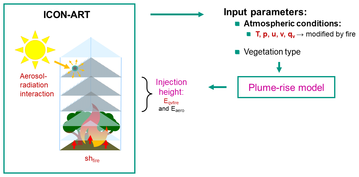
Figure 1 Schematic illustration of the coupling between the plume-rise model and ICON-ART. The diagram shows the sequence of processes: fire-induced sensible heat release, emitted moisture, and aerosol–radiation interaction within ICON-ART, which modify the atmospheric state. These updated conditions are then passed to the Freitas plume-rise model for plume height calculation. Finally, aerosol and moisture is emitted in ICON-ART, and the cycle repeats.

This leads to an emission rate E in kg m⁻² s⁻¹, which is calculated for a respective grid cell and is depending on the height z and the time t.

$$\begin{array}{}\text{(5)}& E(z,t)=M\left(t\right)\times d\left(t\right)\times f(z,t)\times \mathrm{3.4}\end{array}$$

M is the daily mean emission flux in kg m⁻² s⁻¹ based on the GFAS dataset. For this study the aerosol emission flux (E_aero) is assumed to be the sum of the GFAS BC plus OC. d is the diurnal cycle given by Eq. (2) and f is the parabolic emission profile between the upper and lower injection heights. To account for a systematical underestimation of the particulate matter emission in the GFAS dataset, the emission flux is multiplied by an empirical factor of 3.4 as suggested by Kaiser et al. (2012). Later comparisons will demonstrate that the application of this correction factor results in a generally good agreement with observed air quality measurements.

2.1.2 Heat and Moisture Release

In this study, we use the term “fire-induced meteorological changes” to describe modifications, which are induced by fire-related heat and moisture release and/or aerosol-radiation in the ICON-ART model. Thereby, the plume-rise model remains unchanged; it is only influenced by the modified atmospheric state provided by ICON-ART. Figure 1 illustrates how ICON-ART supplies atmospheric input to the plume-rise model. Within the ICON-ART emission routine, the plume-rise model calculates the emission height based on the atmospheric conditions from ICON-ART and the vegetation type of the corresponding grid cell. The plume-rise model internally accounts for latent and sensible heat from the fire as well as cloud formation, but these meteorological changes are not fed back to the ICON host model. Consequently, without the modifications applied in this work, the host model remains unaware, except for the emitted aerosols. In this study, we analyze how incorporating fire-induced heat and moisture release, together with aerosol–radiation interactions, affects atmospheric conditions in ICON-ART and how these changes ultimately influence the calculated plume height, without any tuning of the Freitas model itself.

The parameterizations for heat and moisture release proposed by Muth et al. (2025) are applied and adapted from a convection-resolving to a convection-parameterizing model configuration. Sensible heat release is implemented as a surface-to-atmosphere heat flux within ICON-ART. A brief description of these parameterizations is provided below.

The total energy released by fires is calculated by multiplying the GFAS Fire Radiative Power (FRP) by a factor of 10, as proposed by Val Martin et al. (2012) and applied in Ke et al. (2021). To estimate the portion of this energy contributing to convective processes, a factor of 0.55 is used, following Freitas et al. (2006). Additionally, the FRP is weighted with a diurnal cycle function to account for peak fire intensity typically occurring in the early afternoon. The resulting heat release is implemented as a sensible heat flux from the surface to the atmosphere within the land/surface scheme. ICON-ART then takes this additional heat flux into account when calculating the prognostic variables. The fire-induced sensible heat flux sh_fire defined as:

$$\begin{array}{}\text{(6)}& {\mathrm{sh}}_{\mathrm{fire}}=\mathrm{FRP}\times \mathrm{5.5}\times d\times \mathrm{3.4}\end{array}$$

The FRP and sh_fire both have units of W m⁻². We decided to apply the GFAS correction factor of 3.4 to the heat release estimates as well. Although this factor was originally validated for aerosol emissions only, we extend its application to FRP more broadly. We hypothesize that this adjustment helps compensate for potential underestimations of FRP in cases of intense pyroconvective activity and dense aerosol clouds, which may obscure satellite observations and result in lower FRP retrievals.

The moisture release implementation includes combustion moisture with an emission ratio of 0.75 H₂O $/$ (CO+CO₂) according to Parmar et al. (2008). For the fuel moisture, the burned matter is divided into 30 % dead and 70 % alive components. This follows thresholds from Nolan et al. (2016) and Deb et al. (2020) for southeast Australia and results in an approximate fuel moisture content of 75.42 %.

$$\begin{array}{}\text{(7)}& {\mathrm{qv}}_{\mathrm{fire}}=(\mathrm{0.75}\times (m_{\mathrm{CO}}+m_{{\mathrm{CO}}_{\mathrm{2}}})+\mathrm{0.7542}\times m_{\mathrm{load}})\end{array}$$

The moisture emission flux by the fire is qv_fire in kg m⁻² s⁻¹. m_CO and $m_{{\mathrm{CO}}_{\mathrm{2}}}$ in kg m⁻² s⁻¹ are the mass fluxes of CO and CO₂ from GFAS and m_load in kg m⁻² s⁻¹ is the GFAS combustion rate. The emitted mass is weighted with a diurnal cycle function and again multiplied with the correction factor of 3.4. The moisture is added to the specific humidity tracer in the ICON-ART model. The moisture emission follows the same injection height and profile as the particles, according to the plume-rise model. Therefore, the moisture‑release emission rate E_qvfire can obtained by inserting qv_fire as M in Eq. (5). This additional moisture is added to the existing qv (specific humidity) tracer of ICON and thus, contributes to all physical and dynamical processes. The changes in the atmospheric state by either the heat or moisture release thereby change the atmospheric profiles that are inputs for the plume rise model, and therefore impact the calculated injection height.

2.1.3 Aerosol Optical Properties

As previously noted, ICON-ART incorporates the aging processes of aerosol particles, which significantly influence their optical properties. The methodology employed to represent and simulate this aging is detailed in the following section.

The essential input variables for the ICON-ART radiation calculations include k_ext, ω, and g. These parameters are derived using a Mie code developed by Bond et al. (2006) and Mätzler (2002), based on the work of Bohren and Huffman (2008). Research by Brito et al. (2014) indicates that biomass burning aerosols develop a shell, leading to internal mixing. To account for this particle coating, a core-shell model can be incorporated into the calculations. The input parameters required for the Mie calculations are the median diameter, the shell-to-core fraction, and the refractive index of core and shell. For this study a bi-modal aerosol size distribution with a median number diameter of d_n=20 nm for the smaller Aitken mode and d_n=150 nm for the larger accumulation mode is assumed. The aerosol size distributions and chemical compositions used in this study are consistent with the ranges reported by Brito et al. (2014), based on ground-based measurements during the SAMBBA campaign in September 2012. These findings are further supported by Levin et al. (2010), who investigated the physical, chemical, and optical properties of biomass burning aerosols during controlled combustion experiments in the FLAME campaign. Additionally, Sakamoto et al. (2015) reported similar aerosol characteristics from in-flight sampling conducted with the FAAM research aircraft. Measurements reported by Brito et al. (2014) indicate soluble-to-insoluble fractions of 0.07 and 0.12 for two distinct observational periods. In this study, a shell-to-core volume fraction of 0.1 is adopted, consistent with the range reported by Reid et al. (1998b). Additionally, a BC $/$ OC mass ratio of 0.03, which is within the range reported in Konovalov et al. (2017) is assumed and inorganics $/$ H₂O mass mixing ratio of 0.75. The inorganics-to-H₂O ratio is derived from an analysis of the reference experiment, acknowledging that this parameter is highly uncertain and subject to temporal variability (Zauscher et al., 2013). The results of the Mie calculations is shown in Fig. 2.

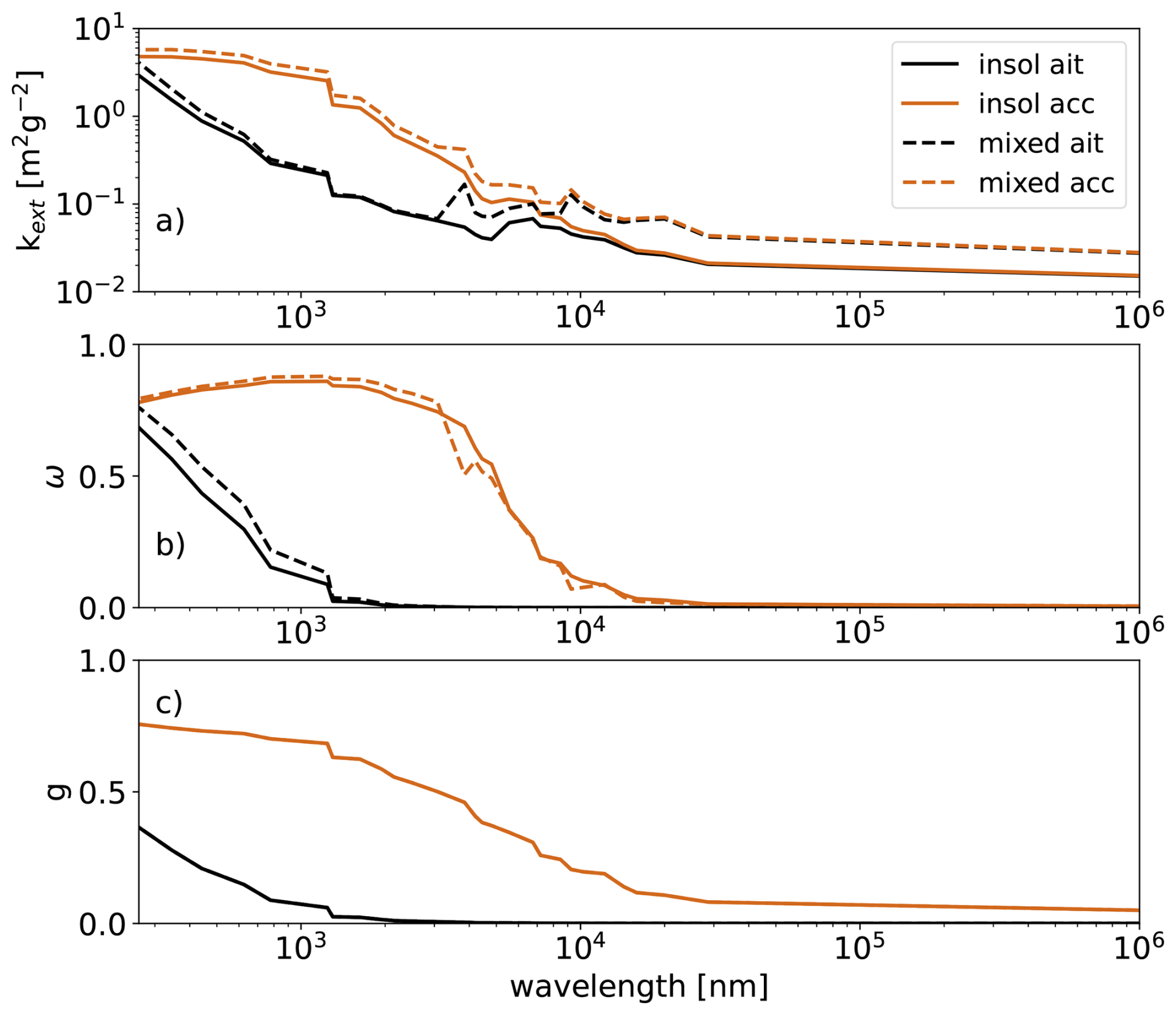
Figure 2 Optical properties of OC+BC containing aerosol modes at ecRad wavelengths. (a) Mass extinction k_ext in m² g⁻², (b) single scattering albedo ω (unit-less), and (c) asymmetry parameter g (unit-less). The black lines show the Aitken mode and the brown lines the accumulation mode. Solid and dashed lines show the insoluble (uncoated aerosol) and mixed (coated aerosol) mode, respectively.

It is evident that the mixed modes (coated aerosol) exhibit higher extinction coefficients and single scattering albedo in the visible range compared to the insoluble modes (uncoated aerosol). This is attributed to the H₂O–H₂SO₄ coating, which acts as a strong scatterer. The Mie theory assumes that particles are spherical. In reality, soot and biomass burning particles have a variety of morphologies: chain aggregates, solid irregulars and more liquid/spherical shapes. The physical and chemical composition is strongly variable and depending on the fuel type, moisture, combustion phase, wind conditions and age of the particles (Reid et al., 1998a). However, the liquid coating can lead to spherical particle surfaces, justifying the assumption of particle sphericity in the mixed mode. For consistency, the sphericity assumption is also applied to the insoluble mode containing uncoated particles, as it is done in Muser et al. (2020).

The calculation of aerosol radiative effects takes place in the ICON-ART model. Aerosol-radiative effects impact the atmospheric stability close to the fire source, which is used by the plume rise model to calculate the emission height, as well as downstream of the plume. Other than the modified atmospheric profiles, the Freitas model does not account for aerosol-radiation interaction.

2.2 Observational data

As a case study, the Australian Black Summer Fires 2019/2020, particularly the initial phase of the Australian New Year's event, has been selected to test the developments. The interaction between the fire, the plumes and the atmosphere during this event was significant. Record-breaking warmth in December, coupled with exceptionally low rainfall, created conditions conducive to extreme fire activity. The ANY event was especially significant due to the passage of a cold front through southeastern Australia. This front was preceded by elevated temperatures and strong wind speeds, which intensified fire behavior. During this event, the fires generated 38 pyroCb clouds, during 18 sub-events (Peterson et al., 2021). This type of intense pyroconvection represents an extreme case and may not be ideal for generalizing fire–atmosphere interactions under typical conditions. However, it provides an excellent opportunity to investigate how extreme wildfires influence meteorological variables and drive plume development.

To validate the results the NASA 3D wind algorithm and CALIPSO data is used. The NASA 3D wind retrieval algorithm, as described by Carr et al. (2018, 2019, 2020), is utilized to determine the heights of plumes and clouds. This algorithm employs stereo imaging, which uses geometric parallax to derive feature heights. By integrating data from geostationary (GEO) and low-earth orbit (LEO) satellites, it produces three-dimensional (3D) atmospheric motion vectors (AMVs) through a multi-platform, multi-angle stereoscopic approach. The term “3D Winds” refers to the three-dimensional positioning of horizontal AMVs within the atmosphere. Observing the parallax of a feature from two different vantage points (stereo) provides direct information about its height.

In this study, the LEO-GEO retrieval method is applied. The LEO satellite data is sourced from Terra and Aqua MODIS Level 1B in the blue band (459–479 nm) with a 500 m resolution. The GEO satellite data is obtained from Himawari-8's blue band (430–480 nm). The Advanced Himawari Imager (AHI), operated by the Japan Meteorological Agency, has a 10 min temporal resolution that is used to track feature movement. MODIS data is then used to calculate parallax, determining AMVs and height. A quality flag is employed to exclude poor retrievals.

Further, analysis of CALIPSO (Cloud-Aerosol Lidar and Infrared Pathfinder Satellite Observation) data is used for validation. The CALIPSO satellite integrates an active lidar instrument with passive infrared and visible imagery to analyze the vertical structure of thin clouds and aerosol layers globally. Launched in 2006 alongside the CloudSat satellite's cloud profiling radar system, CALIPSO provided valuable data on atmospheric clouds and aerosols. The data utilized in this study is the total attenuated backscatter at 532 nm, classified as Level 1 data. These attenuated backscatter profiles are derived from the calibrated, range-corrected, laser energy normalized, and baseline-subtracted lidar return signal. The horizontal resolution ranges from 0.33 to 5 km, while the vertical resolution varies from 30 to 300 m, depending on altitude.

Finally, air quality data from the Centre for Air Pollution, Energy and Health Research’s (CAR) National Air Pollution Monitor Database (NAPMD) were utilized (Centre for Air pollution, energy and health Research, 2021). To reduce noise in the data, three-hourly mean concentrations of PM_2.5 are calculated and compared with corresponding model-derived aerosol concentrations averaged over the respective grid cells. The locations of the monitoring stations are shown in Fig. 3.

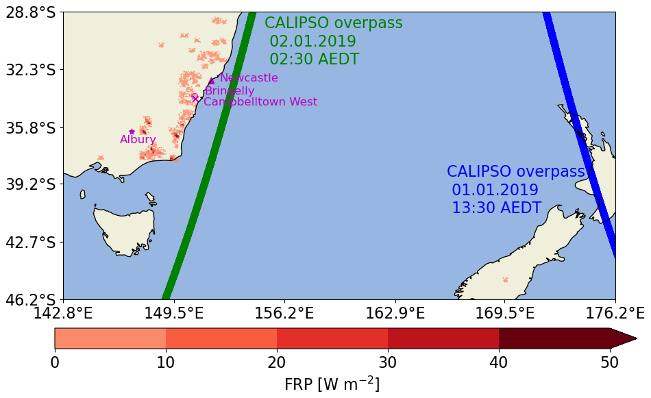
Figure 3 The simulated domain including the GFAS FRP (Copernicus Atmosphere Monitoring Service (CAMS), 2021) remapped to the ICON grid on the 30 December 2019. Generated using Copernicus Atmosphere Monitoring Service information [2023]. The magenta markers show the locations of the air quality stations. The green line shows the CALIPSO overpass on 2 January 2020, at 02:30 AEDT, the blue line corresponds to the CALIPSO overpass on 1 January 2020, at 13:30 AEDT.

2.3 Model Configuration

Prior to the experimental limited-area mode simulations, a global simulation with a grid spacing of 13 km is performed to obtain the input data for the boundary conditions. This global simulation is initialized using the German Weather Service (DWD) analysis product and does not account for fire impacts on the meteorological variables. The limited-area experiment simulations are conducted with a grid spacing of 6.6 km, employing parameterized convection and incorporating a plume-rise model to represent injection heights. It is proposed that at this resolution, the influence of fires on meteorology becomes significant and should not be neglected. However, the grid spacing is still too coarse to explicitly resolve convection and the associated plume-rise processes. The experiment domain extends from southeast Australia to New Zealand, as shown in Fig. 3. The experiments are initialized with the DWD analysis product and meteorological variables of the boundary conditions are read every 3 h. The domain is 30 km high with 70 vertical levels, the vertical grid spacing increases with height. Simulations run from 30 December 2019, at 00:00 UTC to 1 January 2020, at 22:00 UTC and therefore focus on the first phase of the ANY event.

Chemical tracers (CH₄, C₂H₆, C₃H₈, CH₃COCH₃, CO, NH₃, NO₂, SO₂, DMS, HNO₃) are initialized using CAM-Chem data (Buchholz et al., 2019; Emmons et al., 2020). A simplified OH-chemistry mechanism (Weimer et al., 2017) is employed, which additionally includes C₅H₈, CO₂, and OCS. The simulation allows for new particle formation through nucleation, particle coagulation, and condensation of gaseous species. ISORROPIA II (Fountoukis and Nenes, 2007) is used for gas-to-particle partitioning, accounting for H₂O, NO₃, and NH₄. However, secondary organic aerosols are not accounted for.

Emission fluxes for aerosols and the parameterization of moisture and heat release are based on GFAS data (Copernicus Atmosphere Monitoring Service (CAMS), 2021). As mentioned, GFAS has a resolution of 0.1° and is provided on a regular longitude-latitude grid, and therefore needs to be remapped to the ICON triangular grid. This is done using the Radial Basis Function Interpolation. Fire emission data from GFAS is updated daily at 00:00 UTC. The FRP from GFAS is displayed for 30 December in Fig. 3. The GFAS emission flux is proportional to the FRP, indicating fire locations and emission strength. On December 30, the FRP reaches up to 144 W m⁻², on 31 December up to 47 W m⁻², and on 1 January up to 10 W m⁻². This indicates a decrease of fire activity throughout the simulation. In this study, aerosols are treated as an internal mixture of BC and OC to their co-emission from wildfire sources. This representation assumes that both components are part of the same aerosol particle, rather than existing as separate particles. It captures the fact that BC and OC are emitted together and are physically mixed during and shortly after emission. This approach provides a simplified but realistic way to represent wildfire aerosol composition in transport models. 6 % of the particles are emitted in the smaller Aitken mode, with a log-normal distribution around the median diameter of 20 nm and standard deviation of 1.7, and 94 % in the accumulation mode with a with a log-normal distribution around the median diameter of 70 nm and standard deviation of 2.0.

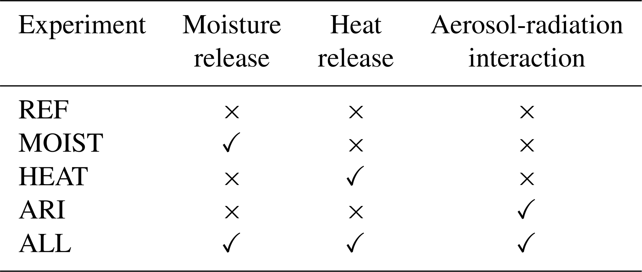
We conducted five experiments (Table 1): a reference run (REF), in which fire aerosol emissions are enabled and the plume-rise model calculates emission heights based on ICON-ART atmospheric conditions without accounting for any fire-induced impacts. In this configuration, aerosol–radiation interactions are not considered, and aerosols are transported as passive tracers. Additionally, three sensitivity experiments were performed based on REF, each isolating a specific process: fire-induced heat release in ICON-ART (HEAT), moisture release in ICON-ART (MOIST), and aerosol–radiation interaction in ICON-ART (ARI). Finally, one combined experiment (ALL) includes all three processes simultaneously.

Table 1 Overview of the performed experiments.

2.4 Definitions and analysis methods

In the following, the evolution of plume is presented. For this analysis, the plume is defined as the set of grid cells in which the aerosol mass mixing ratio exceeds 0.05 µg m⁻³, if not stated otherwise. For vertical profiles within the plume area, the plume area is defined as an aerosol column load exceeding 0.5 g m⁻².

The mass-weighted height is calculated by summing the product of the aerosol mass in each plume grid cell and the corresponding height of the grid cell center. This total is then divided by the overall plume mass to obtain the mass-weighted height.

An additional analysis of surface-based Convective Inhibition (CIN) and Convective Available Potential Energy (CAPE) was performed. Table 2 presents the mean CIN and CAPE values over the fire area derived from the experimental scenarios. The fire area is defined as a grid cell with an aerosol emission larger than $\mathrm{5}\times {\mathrm{10}}^{-\mathrm{12}}$ kg m⁻² s⁻¹, taken from the GFAS dataset. CIN, expressed in J kg⁻¹, quantifies the energy required to lift a surface air parcel to its level of free convection, thereby representing a measure of atmospheric stability. CAPE, also in J kg⁻¹, denotes the amount of buoyant energy available to support convective updrafts, serving as an indicator of the potential intensity of convective processes. For comparison with the NASA 3D wind algorithm, the top height includes contributions from both aerosol plumes and cloud layers, as the retrieval algorithm is unable to distinguish between the two. Therefore, an aerosol plume is defined as a grid cell with an aerosol AOD at 550 nm divided by the vertical extend of the grid cell exceeds a threshold of $\mathrm{50}\times {\mathrm{10}}^{-\mathrm{6}}$ m⁻¹. A cloud is defined as a grid cell in which the combined sum of Liquid Water Content (LWC) and Ice Water Content (IWC) exceeds $\mathrm{0.01}\times {\mathrm{10}}^{-\mathrm{3}}$ g m⁻³. The top height is then determined as the highest altitude level at which either of these thresholds is exceeded.

The comparison between CALIPSO attenuated backscatter and the simulated backscatter reveals several differences. First, the model provides only the total backscatter, not the attenuated backscatter. Second, the simulated backscatter accounts exclusively for wildfire aerosols, excluding contributions from other aerosol sources and clouds. To address the latter limitation, an isosurface corresponding to a combined LWC+IWC of $\mathrm{01}\times {\mathrm{10}}^{-\mathrm{3}}$ g m⁻³ included in the plots. All heights refer to heights above sea level.

3 Results

3.1 Fire-induced meteorological changes in ICON-ART

Firstly, the functionality of the implementations is evaluated. Figure 4a shows the difference in total water vapor column (WVC) (MOIST-REF) at 14:30 AEDT on 30 December. All results are presented in AEDT (Australian Eastern Daylight Time), which corresponds to UTC+11 h. The emission of moisture by the fire causes some noise, especially in areas of smaller fires, but there is an overall increase. In areas with larger fires, the WVC increases by up to 46.6 %. Figure 4b shows the difference in the mean vertical distribution of water vapor concentration (QVC) (MOIST-REF) over the fire area. The areas are divided into three depending on the FRP: the solid line displays the smallest fires with an FRP of up to 25 W m⁻². For these fires, the differences are very small, with maximum increases of 0.003 g m⁻³. For larger fires (25–50 W m⁻²) with the dashed line, the QVC increases up to 0.56 g m⁻², with two peaks around 1 and 5 km. The strongest fires (>50 W m⁻²) show the strongest increase with two peaks, the lower of which is increased up to 1.2 g m⁻³. This shows that the implementation has a notable impact on atmospheric humidity.

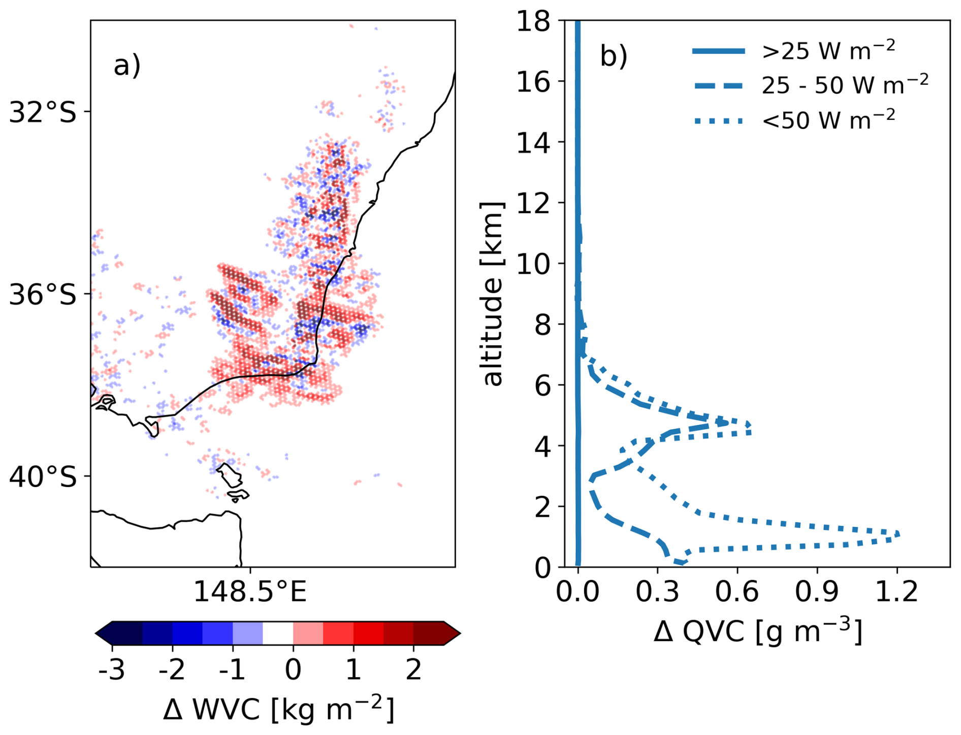
Figure 4 Impact of fire induced moisture release at 14:30 AEDT on 30 December. (a) Difference in WVC MOIST-REF. (b) Mean vertical profile of QVC difference within three different fire areas (MOIST-REF). Solid: 0< FRP >25 W m⁻², dashed: 25 W m${}^{-\mathrm{2}}<$ FRP and FRP >50 W m⁻², dotted: FRP <50 W m⁻².

Figure 5a shows the impact of the heat released by the fire on the 2 m temperature in ICON-ART. The heat release is implemented as a sensible heat flux from the ground to the atmosphere, which strongly affects the temperature beyond other factors. This heat release introduces noise, as well as larger areas of increases of up to 9.3 K, as well as decreases of up to 11.0 K. Here, the areas of increase appear smaller and closer to the fire source, whereas there is a decrease downstream of the fire. This can be attributed to cloud formation and the cloud-radiative effects, which reduce the 2 m temperature in the HEAT experiment and will be discussed in more detail in the following sections. Figure 5b shows the vertical distribution of the mean temperature in the fire area. Again, the effect for fires smaller than 25 W m² (solid line) is minimal, with increases up to 0.1 K. In contrast, fires between 25 and 50 W m² and larger than 50 increase close to the surface by up to 2.1 and 4.0 K, respectively. There are further temperature increases and decreases that can be attributed to dynamics, cloud formation and cloud-radiative effects.

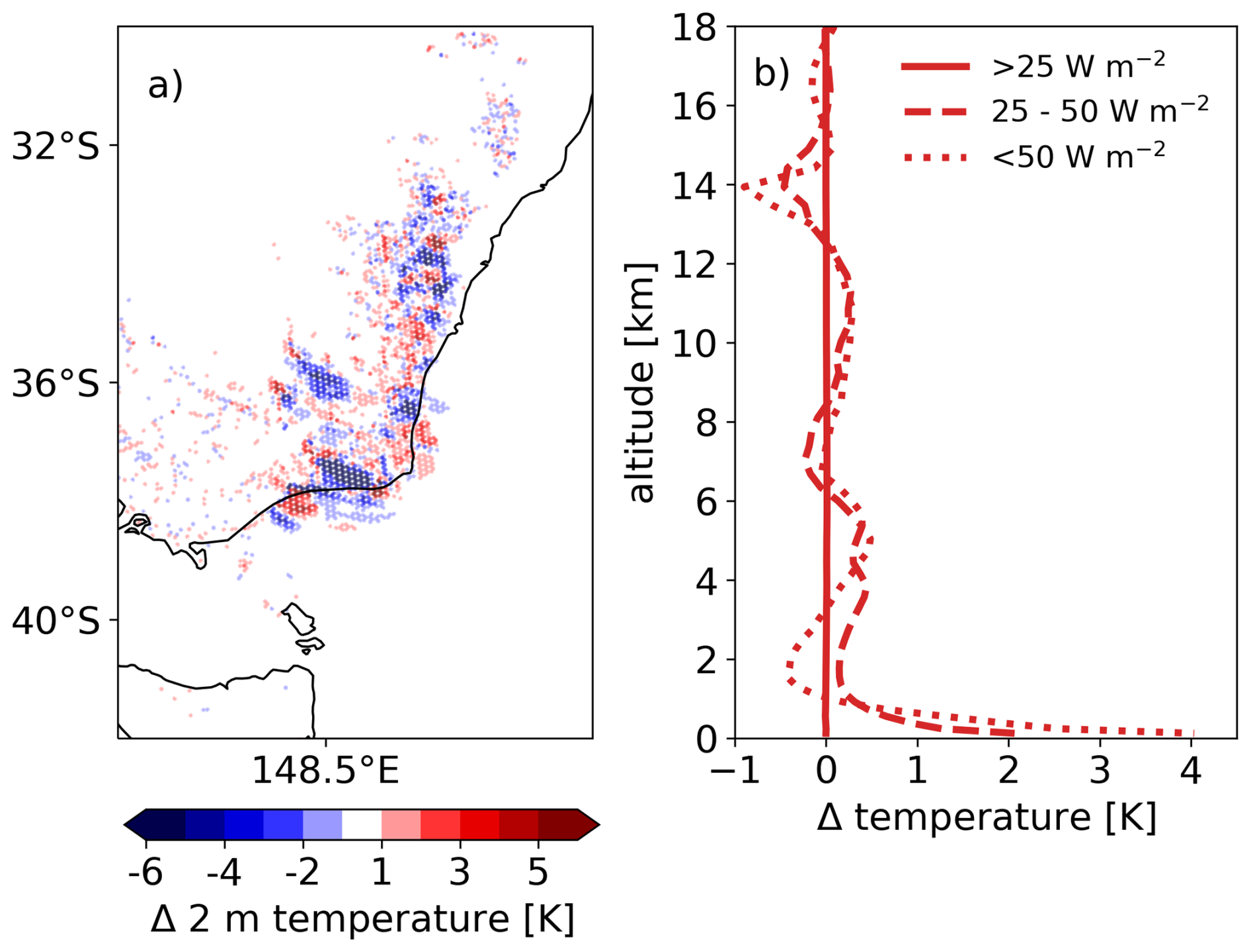
Figure 5 Impact of fire induced moisture release at 14:30 AEDT on 30 December. (a) Difference in 2 m temperature HEAT-REF. (b) Mean vertical profile if temperature difference within three different fire areas (HEAT-REF). Solid: 0< FRP >25 W m⁻², dashed: 25 W m${}^{-\mathrm{2}}<$ FRP and FRP >50 W m⁻², dotted: FRP <50 W m⁻².

Finally, we evaluate the aerosol–radiative effect. Figure 6 illustrates how aerosol–radiation interactions influence vertical wind velocity and temperature within the plume approximately one day after the simulation start. Figure 6a shows that, in the ARI experiment, the probability of stronger updrafts and downdrafts increases, with a more pronounced enhancement in updrafts. This suggests that, compared to the REF experiment, the plume exhibits greater dynamical activity, as well as an overall lofting effect within the plume. Figure 6b presents the mean temperature difference within the plume region. Below 3 km, an overall cooling effect is observed, whereas between 4 and 12 km, there is a warming effect, followed by cooling above 13 km. This pattern indicates warming within the plume core and cooling beneath it. The horizontal distribution of plume-top heights will be discussed later, however, it is important to note that, due to plume lofting, the top heights interacting strongly with radiation vary substantially: from about 2 km up to 16 km. Warming near the plume top is associated with cooling below, and thus spatial averaging significantly smooths these effects.

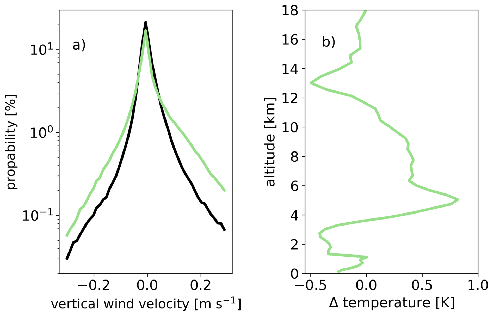
Figure 6 Impact of aerosol-radiation interaction at 14:30 AEDT on 31 December, (a) histogram of vertical wind speeds within the plume area, REF in black and ARI in green, (b) mean vertical profile of temperature difference (ARI-REF) within the plume area.

Overall, Figs. 4–6 illustrate how the ICON-ART meteorology is influenced by the implemented changes and how these modifications in the atmospheric profiles, which serve as input for the Freitas model, can subsequently affect the calculated injection height.

3.2 Comparison to observations

The following section presents a comparative analysis of the different model experiments against observational datasets, including the horizontal and vertical aerosol transport patterns derived from NASA 3D wind retrials and CALIPSO, and the resulting impacts of the ICON-ART modifications on surface-level PM_2.5 concentrations at selected monitoring stations.

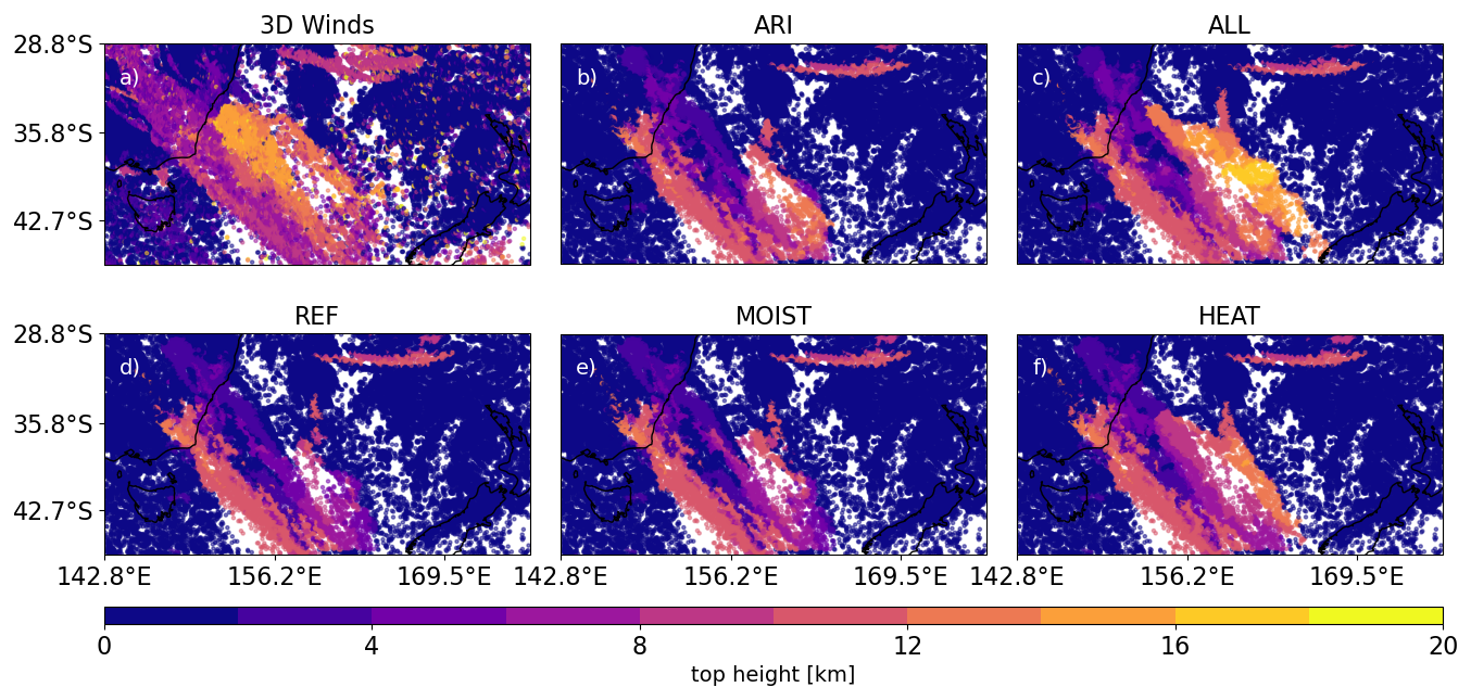
Figure 7 Aerosol and cloud top height on 31 December 2019, at 14:30 AEDT. (a) Retrieved by the NASA 3D wind algorithm. (b–f) Simulated in the experiments: (b) MOIST, (c) ALL, (d) REF, (e) ARI, and (f) HEAT. The dots in panels (b)–(f) represent the top height of either the aerosol plume or a cloud.

Figure 7 shows the 3D wind retrieval compared to the five experiments on December 31st between 13:45 and 15:25 AEDT and the simulation at 14:30 AEDT. The retrieval in Fig. 7a shows a feature almost diagonal through the domain which will be focus of the analysis. Within that feature, there is a convective cell arising southeast of the Australian coastline, with maximum altitudes of 20.0 km. The average heights of the plume and cloud above 2 km are 8.3 km. The REF experiment exhibits similar structural features to those observed in the retrieval. It captures the overlap between the aerosol plume and cloud layers (LWP+IWP is shown in the following section and the plume top height can be found in Appendix B3). Within, there are two distinct elevated regions are evident: one shifted toward the southeast, characterized by both cloud and aerosol presence, and another toward the northwest, dominated primarily by aerosols. The maximum top height within the REF experiment reaches 13.0 km and the average height above 2 km are 6.7 km. This outlines an underestimation of the top heights in REF. The MOIST experiment exhibits similar characteristics to the REF experiment, but with more extensive elevated regions downstream of the plume, outlined by an average top height of 7.0 km and an increase in maximum height of 13.4 km. These results suggest that the release of moisture influences the initial stages of plume development; however, its overall impact on the vertical structure remains limited. The ARI experiment also exhibits similarities to the REF experiment but demonstrates enhanced plume elevation downstream, with a maximum top height of 13.0 km and an average top height of 7.3 km. After the emisssion in ICON-ART, aerosol–radiation interactions contribute to a gradual rise in plume altitude over time. Initially, the top heights in the ARI experiment are underestimated; however, as the plume ascends due to these interactions, the top heights increasingly align with observational data, showing improved agreement compared to the REF experiment. In the HEAT experiment, a pronounced elevation of the plume is observed downstream of the coastline, closely matching the spatial distribution seen in the observations. The maximum top height reaches 14.4 km, with an average top height of 7.6 km. Although an underestimation remains, the release of sensible heat in the ICON-ART model increases the buoyancy and and emission initial emission height, which improves the transport and the HEAT experiments aligns agreeably with the observations. In the ALL experiment, a dominant elevation is simulated southeast of the Australian coast, with a maximum altitude of 18.0 km and an average top height of 8.6 km, aligning even better with the observations. The maximum plume height is still underestimated; however, the retrievals reach altitudes of up to 20 km in localized regions. In contrast to this underestimation, the average top height exceeds the observed value by 0.5 km. Nevertheless, the initially increased buoyancy and through heat and moisture release, combined with lofting induced by aerosol–radiation interactions in the ALL setup, effectively reproduces the observed patterns.

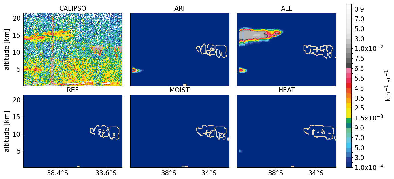
Figure 8 CALIPSO attenuated backscatter at 532 nm and simulated backscatter at 532 nm on 1 January 2020, at 13:30 AEDT. (a) CALIPSO data. (b–f) Simulated in the experiments: (b) MOIST, (c) ALL, (d) REF, (e) ARI, and (f) HEAT. The light yellow line displays the $\mathrm{0.01}\times {\mathrm{10}}^{-\mathrm{3}}$ g m⁻³ LWP+IWP isosurface.

The CALIPSO attenuated backscatter at 532 nm is compared to the simulated backscatter from the experiments (Fig. 8), along a satellite overpass near New Zealand on 1 January 2020, at 13:30 AEDT, see Fig. 3. The CALIPSO cross-section reveals signal centered around 15 km altitude, accompanied by a second feature near 5 km in the southern portion of the transect, both classified as a mixture of cloud and aerosol. Additionally, a signal is visible above 10 km in the northern half of the overpass, classified as cloud. The near-surface signal is primarily classified as marine aerosol with localized cloud contributions. Our simulations only account for wildfire aerosols; therefore, the absence of background signals and the maritime aerosol layer is expected. The lack of clouds can be explained by the omission of aerosol–cloud interactions in the model configuration close to the surface. Other discrepancies also fall into the expected range. In the REF and MOIST experiments, no aerosol backscatter is simulated. However, the simulated $\mathrm{01}\times {\mathrm{10}}^{-\mathrm{3}}$ g m⁻³ LWP+IWP isosurface around 10 km aligns with the observed cloud structures, and some low-level clouds are also simulated. The HEAT experiment captures the cloud signals and shows a small aerosol signal at the southern border of the shown overpass, indicating that the initially increased injection height improves aerosol transport compared to observations. However, the signal is underestimated in size, which can be attributed to a general underestimation, or as the overpass is along the edge of the plume (see Figs. 3 and 7) the simulation slightly mismatches the transport. The ARI experiment successfully reproduces the observed cloud signals. Additionally, an aerosol backscatter signal around 5 km is present at the southern edge of the overpass, consistent with CALIPSO observations. This suggests that a lofting mechanism is necessary and more effective than an increased emission height to transport aerosols to the observed location. The ALL experiment captures the cloud layer at 10 km but lacks near-surface cloud features. The aerosol backscatter matches the observations well, reproducing both the signal at 5 km and the elevated layer at 15 km. Overall, the findings highlight the limited impact of fire-induced moisture on aerosol transport in the MOIST experiment. The absence of a signal in the HEAT experiment suggests that, despite a higher initial emission profile, aerosol lofting is essential for transporting particles into the UTLS. Moreover, the signal around 5 km underscores the importance of lofting processes at lower altitudes. The comparison of ALL and ARI outlines an increased lofting effect of for and initially higher injection height. It should be noted that no clouds are simulated within the regions containing aerosol in the model output. Given reports of potential misclassifications of dense aerosol plumes in high altitudes (Liu et al., 2019), it remains unclear whether this discrepancy arises from limitations in the simulation (e. g. missing aerosol-cloud interactions) or from flaws in the observational classification. The absence of low-level clouds in the ALL experiment further underscores the semi-direct aerosol effect, where stabilization through aerosols-radiation interaction suppresses cloud formation.

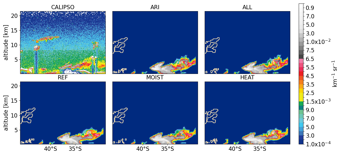
Figure 9 CALIPSO attenuated backscatter at 532 nm and simulated backscatter at 532 nm on 2 January 2020, at 02:30 AEDT. (a) CALIPSO data. (b–f) Simulated in the experiments: (b) MOIST, (c) ALL, (d) REF, (e) ARI, and (f) HEAT. The light yellow line displays the $\mathrm{0.01}\times {\mathrm{10}}^{-\mathrm{3}}$ g m⁻³ LWP+IWP isosurface.

Figure 9 presents the CALIPSO 532 nm attenuated backscatter cross-section south of the Australian coast on 2 January 2020 at approximately 02:30 AEDT. The satellite data reveals backscatter between 2 and 5 km, with additional features at 10 km (31° S), 8 km (34° S), and 12 km (between 43 and 38° S), all classified as clouds by the CALIPSO algorithm. The model simulations also reproduce cloud structures in these regions, including those south of 43° S. The REF experiment aligns well with the observations, capturing the signals below 2 km north of 43° S. The signal north of 38° S matches well in both height and magnitude. The LWP+IWP isosurface matches, although shifted to the south with the detected cloud signal. The other experiments show similar results to REF and therefore also align well with the observations. This agreement indicates that the baseline model configuration is sufficient to reproduce the observed plume structure under these conditions. The similarity between REF and the other experiments (MOIST, ARI, HEAT, and ALL) suggests that fire-induced meteorological changes have a limited influence on plume height for this overpass.

Therefore, the differences between the two CALIPSO observations need to be discussed. Firstly, the age of the plume is different. In Fig. 9, the plume is close to the source on 1 January. It has been established that on this day the FRP is smallest, resulting in lower moisture, heat release, and aerosol emission. Secondly, the overpass occurs during the night, when the atmosphere is more stable. This generally decreases vertical transport in all experiments. The diurnal cycle reduces heat and moisture during the night further, and the aerosol-radiative effects are limited to terrestrial radiation and remain small. All these factors reduce the impact of the implemented features, leading to similar results. However, the good agreement with the observations and the significant decrease in fire and moisture release indicate that for less intense fires, the plume-rise model performs well without the additional implementations. Therefore, it can be concluded that the fire's impact on the meteorology in the host model can be neglected for small to moderate fires. However, for extreme events, these effects are crucial.

So far the focus has been on the plume development and height but we further want to analyze how the different emission profiles impact the surface-level air quality. Figure 10 compares simulated wildfire aerosol concentrations below 2.5 µm in diameter with observed PM_2.5 measurements at several monitoring stations (locations shown in Fig. 3). It is important to note that, the measurements reflect total particulate matter, including non-wildfire sources not represented in the model. These factors introduce inherent uncertainties in the comparison. However the close proximity of the stations to fire areas (Fig. 3) suggests that wildfire aerosols are the dominant source. At Station Albury, all simulations tend to underestimate PM2.5 concentrations; however, the observed peak on 31 January is reasonably well captured, except for the HEAT experiment. At Stations Bringelly and Campbelltown West, which are located near the emission source and in close proximity to one another, the REF and MOIST and HEAT experiments overestimate observed concentrations. In contrast, the ARI, and ALL experiments show improved agreement with measurements, indicating that the inclusion of fire-induced processes helps constrain near-source concentrations. At Station Newcastle, inter-experiment variability is minimal, with consistently lower concentrations in the HEAT, ARI, and ALL experiments. Overall, the simulations reproduce the observed concentration patterns reasonably well, thereby validating our assumptions regarding the aerosol emission flux, which consists of BC and OC, using a correction factor of 3.4.

However, point-to-point comparisons remain sensitive to small discrepancies in simulated plume height and transport pathways, which can lead to substantial local deviations. This is particularly evident at Stations Bringelly and Campbelltown West, where, despite their close spatial proximity (approximately 20 km), the temporal evolution of concentrations differs markedly, underscoring the complexity of near-source plume dynamics In summary, the impact of varying experimental configurations appears to be non-linear. In some cases, enhancements such as heat release lead to a reduction in near-surface aerosol concentrations, whereas in others, concentrations increase. Notably, at the Bringelly and Campbelltown West stations, the overestimations observed in the REF, MOIST, and HEAT experiments are mitigated in the ARI and ALL setups, highlighting the importance of lofting for accurate near-source air quality representation.

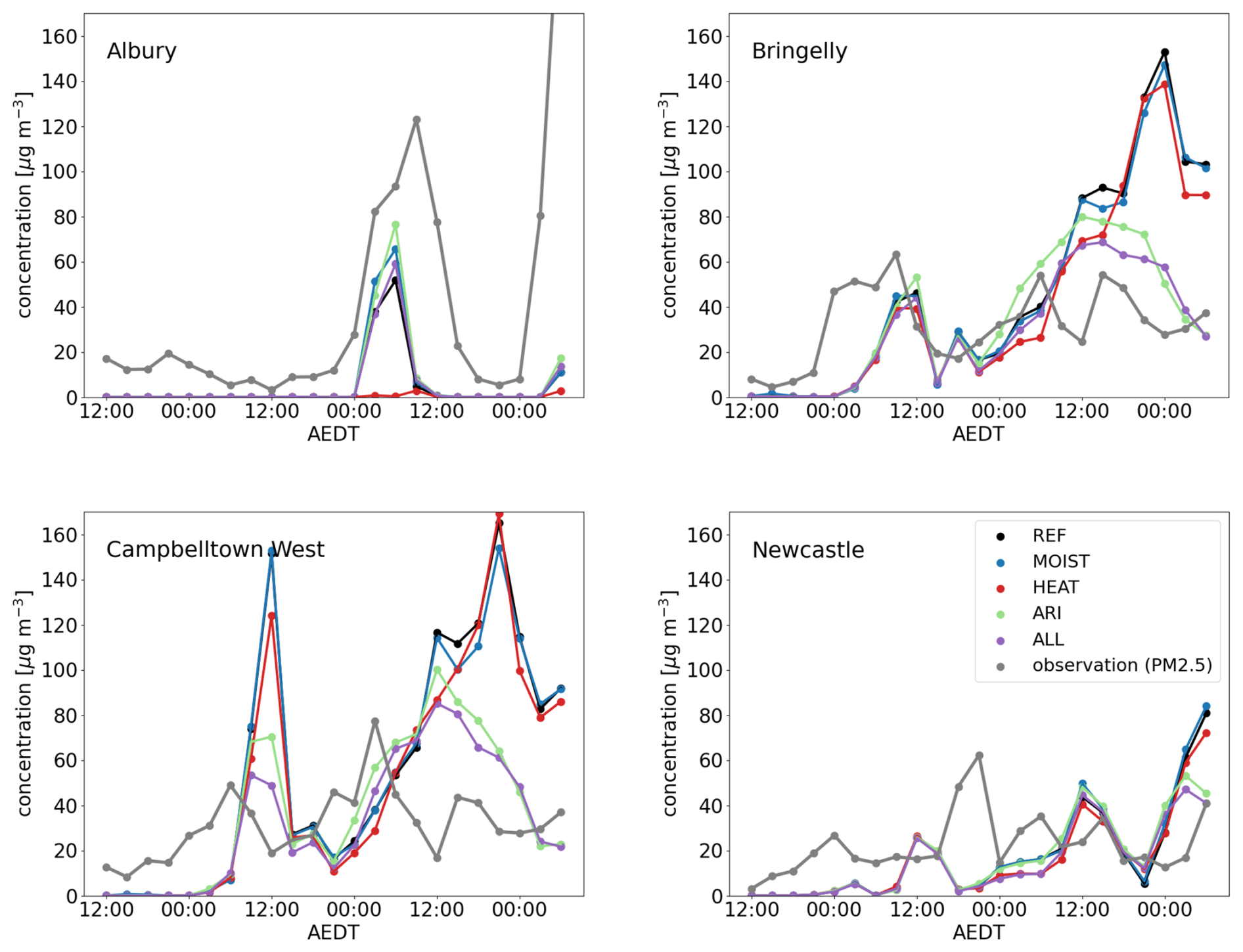
Figure 10 Comparison of 3 h mean PM_2.5 air quality measurements and simulated ICON-ART aerosol at four different locations, shown in Fig. 3. Observations are shown in gray, the simulation REF in black, MOIST in blue, HEAT in red, ARI in light green, and ALL in purple.

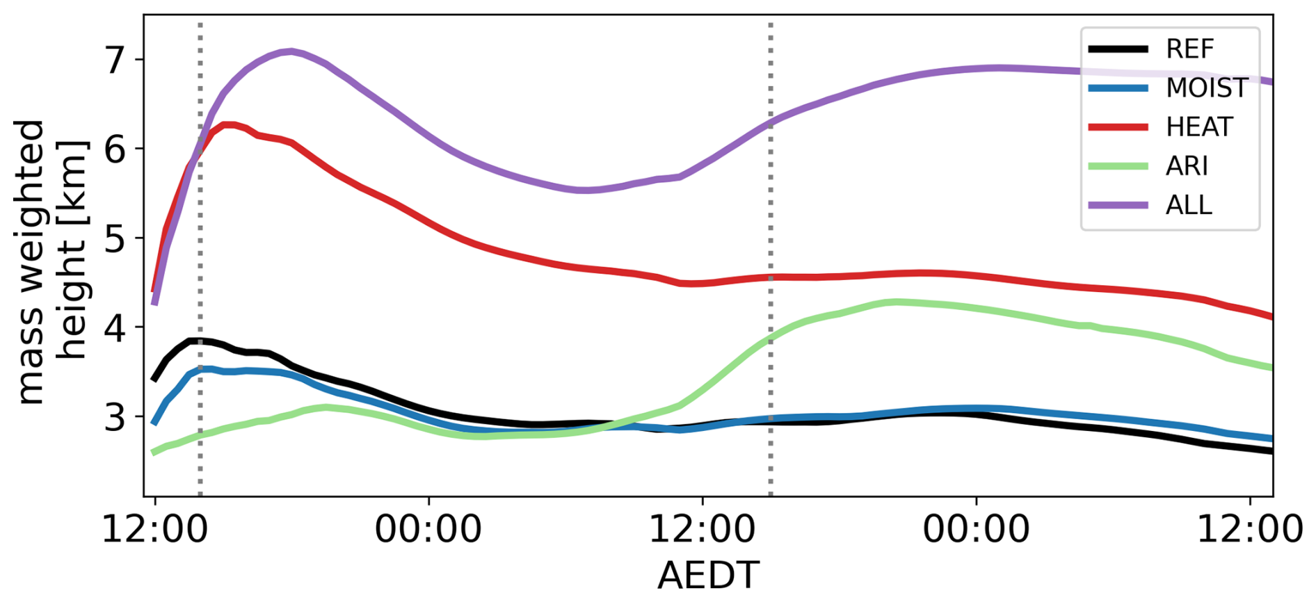
Figure 11 Temporal evolution of mass weighted height of the plume during the first two simulation days. REF is in black, MOIST in blue, HEAT in red, ARI in green, and ALL in purple. The gray dotted lines indicate 14:30 AEDT on 30 and 31 December.

3.3 Impact of Fire-induced atmosphere changes on Plume and Clouds

The comparison with observations established, that accounting for heat and moisture release, as well as aerosol-radiation interaction in ICON-ART improves the simulation. The different mechanisms are analyzed in the following.

Figure 11 illustrates the plume mass-weighted height for the performed experiments. In the REF experiment, the mass-weighted height increases to a peak at 3.8 km after 4 h, and declines by 1.2 km within the next 48 h. Since the ICON-ART meteorological input remains unaffected by the fire, the evolution of the calculated injection heights during the first day is driven by the typical diurnal cycle of atmospheric stability, which decreases throughout the day due to increased solar radiation. This destabilization is reflected in the ICON-ART atmospheric profiles used by the plume-rise model to calculate emission height, together with the diurnal cycle of fire intensity assumed in the plume-rise model. The combination of increasing fire intensity and decreasing atmospheric stability during the day leads to higher plume heights. As previously explained, FRP and consequently the emission strength decreases over the time span of the simulation. Therefore, the mass-weighted plume height is primarily influenced by emissions occurring during the first day of the simulation. The decline observed after the peak can be attributed to sedimentation processes and emissions occurring at lower altitudes. The MOIST experiment follows a similar evolution as REF, but with a lower peak at 3.5 km after 3.5 h. The impact of water vapor release is greatest on the first day, when emissions are strongest, and has no significant impact on the overall mass weighted height development thereafter. In contrast, the HEAT experiment shows substantially higher values, peaking at 6.3 km after 4.5 h, and minimum values of 4.0 km after two days. This can be explained by two main factors. First, the sensible heat release by the fire destabilizes the atmosphere and creates buoyancy, which lifts the plume within ICON-ART higher and second, this less stable atmosphere in ICON-ART is now used by the plume-rise model to calculate the injection height, thereby increasing the height. The effect is strongest on the first day, as it is proportional to the FRP. Constant emissions at lower levels and sedimentation decrease the mass-weighted height thereafter. The ARI experiment starts with the lowest mass-weighted height. This can be explained by the absorption of solar radiation by the dense aerosol plume above the fire area. This leads to a stabilization of the atmosphere in ICON-ART over the fire area, which reduces the calculated injection height by the plume-rise model. The maximum height of 4.3 km is observed on 31 December at 20:30 AEDT. The scattering and mainly absorption of solar radiation can warm the plume top and create buoyancy within ICON-ART. The ALL experiment exhibits the most pronounced plume development, the top height of 7.1 km is reached after 5 h, followed by a decrease during night and an increase after noon. This shows that destabilization due to the sensible heat release counteracts the stabilizing effects of additional cloud formation and aerosol-radiation interaction in ICON-ART. It appears that the lofting effect in comparison to ARI is increased, outlining again a correlation of the lofting effect with the injection height. The aerosol radiative effect is modulated by both cloud cover and the relative positioning of the aerosol plume. The initial lofting, driven by fire-induced heat and moisture release, increases the area of the plume exposed to solar radiation. This enhancement is attributed to the elevated initial plume height, its positioning above optically thick clouds, and a broader horizontal distribution.

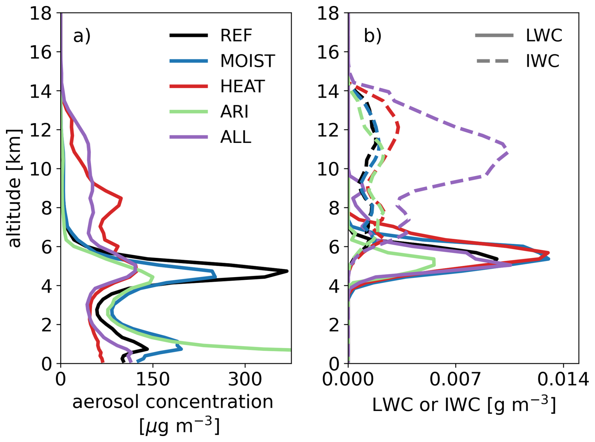
Figure 12 Mean vertical profile within the fire area at 14:30 AEDT on 30 December. (a) Aerosol concentration. (b) LWC (solid line) and IWC (dashed line). The profiles are color-coded as follows: REF (black), MOIST (blue), HEAT (red), ARI (light green), and ALL (purple).

To explain the initial difference in mass-weighted height Fig. 12 illustrates the mean vertical profile of the mean aerosol concentration over the fire area in (a) and LWC and IWC over fire area in (b), on 30 December at 15:00, 2 h after peak fire intensity in the simulation. In Fig. 12a, the REF experiment shows two peaks in the aerosol concentration: the maximum at 4.7 km and a local peak at 0.7 km. The mean LWC and IWC in Fig. 12b shows, that in the REF experiment clouds form between 3.5 and 14.4 km, with a peak condensate at 5.4 km. This indicates some convection, at least in parts of the fire area, which can further be connected to the passing cold front and the thereby caused instability. The aerosol concentration in the MOIST experiment also shows two peaks, however the upper peak is reduced by 31.6 %, while the lower peak increases by 39.3 %. IWC and LWC also show a similar distribution as REF. However, the peak of LWC increases by 30 %. It is shown that additional water vapor leads to more cloud formation in areas of preexisting clouds. The additional energy from the latent heat release, which is hypothesized to lift the aerosols higher, is counteracted by the stabilization of the atmosphere due to cloud radiative effects. This more stable atmosphere is now used by the plume-rise model to calculate the emission height. The aerosol concentration in the ARI experiment again shows two peaks. In comparison to REF and MOIST, the maximum is closer to the surface at 0.2 km height with a mean concentration more than twice as high as the REF maximum. Further, in the ARI experiment, there is an overall decrease in LWC, with a reduced mean of 50 % at 5.4 km. This reduction indicates a stabilization of the atmosphere due to aerosol-radiation interaction, and results in most of the aerosol plume remaining close to the surface. The IWC remains comparable to the REF experiment. The aerosol distribution in the HEAT experiment exhibits a markedly different vertical profile, characterized by a more stratiform structure with emissions reaching up to 13.9 km. Notably, two smaller peaks at 4.7 and 8.5 km are observed, with a maximum concentration of 121.5 µg m⁻³. Additionally, cloud formation increases. The LWC rises to levels comparable to those in the MOIST experiment. A local maximum at 12.1 km further indicates enhanced cloud ice formation, suggesting that clouds can develop even in the absence of additional moisture. In the ALL experiment, the vertical aerosol distribution shows emissions extending up to 14.8 km. The concentration peaks at 5.0 km; however, due to the more uniform profile, this peak is reduced by 67 % compared to the REF experiment. Near-surface concentrations are only slightly reduced by up to 19 % relative to REF. This highlights, on one hand, the increased buoyancy resulting from heat release and enhanced convection, and on the other hand, the stabilizing effects of aerosol- and cloud-radiation interactions. The ALL experiment integrates all contributing factors, producing the strongest cloud response. Although the peak at 5.5 km increases only slightly, the LWC shows a consistent rise to up to 9.9 km. The IWC exhibits a distinct local maximum at 10.8 km, with peak concentrations increasing by a factor of 5.7 compared to REF. It is important to note that the presented profiles represent spatial averages; thus, the stabilizing effects are more pronounced in regions with smaller fires, while increased convective cloud formation is observed in areas with higher emissions and more intense fires. Furthermore, a considerable amount of aerosols is emitted above the cloud peak concentration level in the ALL experiment, whereas in the ARI experiment, the majority of aerosols remain below the cloud layer. This suggests that the lofting effect in the ALL experiment may be stronger due to less absorption and scattering of solar radiation by clouds above the aerosol layer, allowing more energy to reach and heat the aerosol layer, thereby enhancing vertical transport.

Additionally, the influence of the different experimental setups on surface pollutant concentrations is noteworthy, given the substantial impact of wildfire emissions on air quality. The results suggest that the stabilizing effects of aerosol- and cloud-radiation interactions lead to elevated surface concentrations compared to scenarios dominated by heat release. However, this was only observed at station Albury.

Table 2 Mean CIN and CAPE in the fire areas for the REF, MOIST, HEAT, ARI, and ALL experiments on 30 December, 15:00 AEDT. The values are given J kg⁻¹.

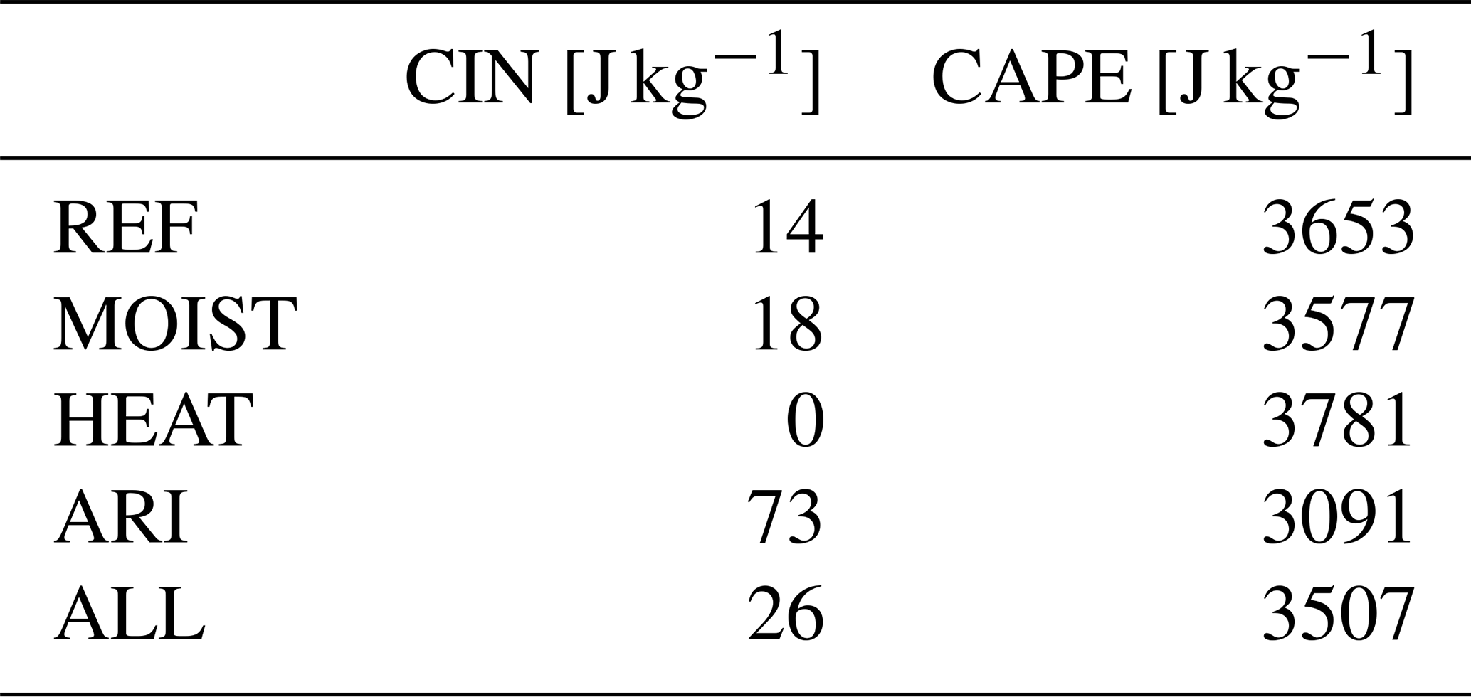
In the next step, the impact of the different experiments on atmospheric stability in ICON-ART is examined. Table 2 indicates that all experiments exhibit atmospheric instability within the fire areas, with CAPE values suggesting the potential for deep convection. However, the interplay of fire-induced effects including moisture release, heat fluxes, and aerosol–radiation interactions leads to notable variations in both CIN and CAPE. These variations reflect the complex feedback mechanisms between the emissions and convective processes. In the REF experiment, CIN is 14 J kg⁻¹ and CAPE is 3653 J kg⁻¹, providing baseline conditions for convective development. The addition of water vapor in the MOIST experiment slightly increases CIN to 18 J kg⁻¹ and decreases CAPE to 3577 J kg⁻¹. Increased humidity generally leads to more rapid saturation of rising air parcels, resulting in the release of latent heat. As a consequence, the parcel becomes positively buoyant, meaning it is more capable of rising through the atmosphere. Thus, CIN/CAPE should decrease/increase as humidity increases. Figure 12 also indicates an increase in cloud formation, which contributes to atmospheric stabilization through cloud radiative effects. This stabilization is primarily associated with surface cooling due to reduced incoming solar radiation. Nevertheless, the overall changes remain small. The ARI experiment exhibits the highest CIN (73 J kg⁻¹) and the lowest CAPE (3091 J kg⁻¹), consistent with aerosol–radiation interactions stabilizing the lower atmosphere and suppressing convective activity. In contrast, the HEAT experiment shows the strongest convective potential, with no inhibition (CIN = 0 J kg⁻¹) and the highest CAPE (3781 J kg⁻¹), suggesting that fire-induced heating strongly promotes convective initiation and vertical development. In the combined experiment ALL, CIN is 26 J kg⁻¹ and CAPE is 3507 J kg⁻¹, reflecting the net effect of competing processes. Again, the values represent area-averaged quantities. The high CIN values indicate the presence of regions with increased atmospheric stability, typically associated with smaller fires. In contrast, larger fires exhibit substantial heat release, which counteracts the stabilizing effects and promotes convective activity.

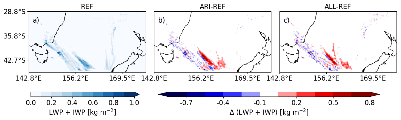
Figure 13 LWP+IWP for the (a) REF, difference in LWP+IWP for (b) ARI-REF, and (c) ALL-REF on 31 December at 14:30 AEDT.

In a next step, the impact of aerosol-radiation interaction on the cloud development downstream of the plume is analyzed. Figure 13a displays the sum of LWP + IWP for the reference experiment. The individual contributions of LWP and IWP are shown separately in Appendix B1 and B2. A cloud band spreads from the northwestern corner southeast through the domain, overlapping with the aerosol plume. This cloud band is associated with a front passing through. Figure 13b shows the difference of ARI – REF. There is noise within the cloudy areas, but significant increases in LWP + IWP are observed in the southeastern region of the cloud band. This clear increase stems from an increase in liquid clouds forming due to the aerosol-radiative effect. West of the cloud band, there is an increase in cloud ice caused by aerosol-radiative effects. Figure 13c shows the differences between ALL and REF. Again, there is noise, but also areas of increase. The areas of increase are evident in the southeastern part of the cloud band and east of the cloud band where the plume is located. The increases within the cloud areas are predominantly in liquid clouds, while east of the cloud band, there is a dominant increase in cloud ice. Therefore, aerosol-radiation induced plume warming increases the buoyancy of rising air parcels, allowing the plume to ascend higher and promote cloud formation. In contrast to the beginning of the simulation, where the dense aerosol plume induces atmospheric stabilization. This highlights the semi-direct aerosol effect, which can exert both stabilizing and destabilizing influences on atmospheric dynamics, depending on the vertical distribution and optical thickness of the aerosol plume. When aerosols absorb solar radiation, they can heat the surrounding air, potentially stabilizing the lower atmosphere by suppressing convection. This effect tends to trap pollutants near the surface, enhancing surface concentrations, as seen close to the source. Conversely, if the aerosol layer is elevated and sufficiently dense, it can destabilize the atmosphere by creating temperature gradients that promote vertical mixing. The net impact of the semi-direct effect is therefore highly sensitive to plume height, aerosol concentration, atmospheric stratification and the aerosol optical properties. Furthermore, a distinction between the ARI and ALL experiments is evident. While some of these differences can be attributed to initial conditions, such as the plume injection profile, the vertical positioning of the aerosol plume relative to cloud layers further contributes to the observed discrepancies.

4 Discussion

4.1 Uncertainty in model configuration and parameterization

Previous studies have documented limitations of the Freitas plume-rise scheme (Val Martin et al., 2012; Wilmot et al., 2022; Wang, 2024), notably its tendency to underestimate the dynamic range of injection heights. Our results confirm this bias for high-intensity fires. To evaluate these limitations, we employed a configuration with 6.6 km horizontal resolution that does not explicitly resolve deep convection. This choice provides a stringent test of a parameterization originally designed for coarser grids (∼100 km). While underestimation of plume heights has been documented for plume-rise models, including Freitas, attributing this bias solely to the parameterization may be overly simplistic. Heat-flux density – a key driver of plume buoyancy – is poorly constrained outside of limited field campaigns. Satellite-derived fire products, which provide the majority of input data, may systematically underestimate this quantity, complicating the interpretation of model–observation differences. Enhancements such as fire-induced meteorological changes within the ICON framework may partly compensate for low-biased inputs rather than exclusively correcting physical parameterizations. However, this study aims to develop a model setup that can be applied globally and in near real time, and is therefore restricted to suitable available datasets and the information they provide which as of right now are based on satellite data.

The emission estimates are subject to several uncertainties. First, the emission profile, which is assumed to be parabolic, whereas studies such as (Moisseeva and Stull, 2021; Wilmot et al., 2022) indicate that the majority of aerosols are concentrated near the plume top. However, when considering the fire's impact on meteorology, additional vertical transport within the host model enhances upward motion and therefore aerosol transport toward the plume top, which may partially correct this discrepancy. Second, Eq. (1) assumes a linear relationship between FRP and burned area, which may not hold in all cases. For example, although forest fires typically burn smaller areas than grass fires, they can exhibit higher FRP due to denser fuel loads (Zheng et al., 2021). Next, applying a typical diurnal cycle function introduces uncertainties that vary across different climate zones and fire regimes. Weighting the diurnal cycle according to vegetation type is an important first step; however, impacts like combustion phases, for example, are neglected. Additionally, in contrast to the typical diurnal pattern of atmospheric stability and fire intensity – where pyroCb clouds generally form in the early to late afternoon – some of the most intense pyroCb activity during the ANY event occurred at night (Peterson et al., 2021). This discrepancy between the expected diurnal cycle of atmospheric stability, fire intensity, and observed nighttime pyroCb activity is not captured in the simulation and is discussed in more detail in Muth et al. (2025), and can also be seen in Appendix A1. Furthermore, GFAS inputs derived from MODIS FRP are subject to cloud and smoke interference, view-angle effects, and potential sensor saturation, all of which bias fire intensity estimates low (Kaiser et al., 2012). The conversion of the FRP into emission factors introduces additional uncertainties. The conversion from FRP to convective heat flux relies on empirical coefficients that vary with fuel type and combustion conditions (Val Martin et al., 2012). Moisture release estimates introduce additional uncertainty, as weighting factors in Eq. (7) are based on fuel-moisture characteristics from Nolan et al. (2016) and Deb et al. (2020) for southeast Australia, they may not be generally applicable. For particulate matter, Kaiser et al. (2012) shows that there is a systematical underestimation by GFAS and therefore introduces a correction factor of 3.4. We also applied this factor to our aerosol emissions, and based on Fig. 10, the application of this factor shows overall good agreement with observations. This factor was empirically derived for particulate matter and may be attributed either to uncertainties in the emission parameterization, which can be substantial (Urbanski, 2014), or to a general underestimation of the FRP on which the parameterization is based. The comparison of direct MODIS FRP measurements with the FRP assumed in ICON, both with and without the 3.4 emission factor (see Appendix A1), demonstrates that applying the enhancement factor improves the agreement between the assumed FRP and MODIS observations. Although this does not constitute proof that the enhancement factor is universally applicable due to systematic underestimation, it can reasonably be assumed for the case considered here.

4.2 Subgrid treatment of fire forcing.

Fire-induced heat and moisture release were distributed uniformly across each grid cell, rather than applied at subgrid scale, as proposed by Ma et al. (2025). In their approach, fire heat was explicitly represented within the superparameterized Community Earth System Model (SP-CESM), which embeds 2-dimensional cloud-resolving models (CRMs) at 4 km resolution inside each GCM grid cell. Fire heat fluxes were applied only to a subset of CRM columns proportional to the burned area, creating horizontal heterogeneity and localized buoyancy maxima that drive secondary circulations and more realistic convection. In our simulation the grid spacing of 6.6 km is comparable to the 4 km resolution of the CRMs. Further, the GFAS input resolution (0.1°, ≈11 km) allows no further subdivision. Nevertheless, neglecting localized buoyancy maxima may dilute effective heat-flux density and can reduce injection heights. However, injection height is parameterized within the plume rise model, and the implementation of heat and moisture release in ICON-ART allows for an averaged fire effect on meteorological variables in the host model, ensuring that large-scale atmospheric responses to fire heat are still represented.

4.3 Aerosol–radiation interactions

Biomass-burning aerosols exert significant radiative effects on plume dynamics, including plume rise (Ohneiser et al., 2023). These effects depend strongly on aerosol optical properties, which in turn vary with OC $/$ BC ratios, vegetation type, combustion efficiency, and fuel moisture (Janhäll et al., 2010). Higher BC fractions enhance absorption and reduce the single scattering albedo, whereas higher OC fractions increase scattering. In this study, aerosols are represented as internally mixed particles with fixed optical properties, a simplification that neglects dynamic aging processes such as condensation, coagulation, and chemical transformation (Seinfeld and Pandis, 2006). These processes alter size distribution, refractive index, and hygroscopicity, and recent observations indicate that stratospheric BC particles are heavily coated with organics during pyroCb events (Beeler et al., 2024). Furthermore, assuming spherical morphology introduces substantial error: Romshoo et al. (2022) report overestimations of the single scattering albedo by up to a factor of five and absorption coefficients by up to a factor of three. Incorporating morphology-aware optical models and dynamic mixing-state representations would improve accuracy, particularly for fresh emissions undergoing rapid chemical processing.

4.4 Aerosol–cloud interactions

Aerosol–cloud interactions, which influence pyroCb formation, were not represented. While some studies report enhanced updrafts due to increased CCN concentrations (Andreae et al., 2004; Koren et al., 2005; Wang et al., 2009), others find limited dynamical impact compared to fire-generated heat fluxes (Luderer et al., 2006; Kablick III et al., 2018). Based on these findings, we assume aerosol–cloud interactions exert a secondary influence relative to meteorological impacts in our simulations.

4.5 Comparison with observations

Uncertainty in observational benchmarks further complicates evaluation. NASA 3D wind retrievals carry height uncertainties of ±200–300 m, consistent with Carr et al. (2019), and depend on LEO–GEO viewing geometry. Detection thresholds for plume/cloud identification are not standardized, introducing ambiguity in comparisons. Model vertical resolution (200–250 m between 9–15 km) is comparable to observational error but increases with altitude, potentially biasing analysis toward higher levels. Despite these limitations, the adopted approach provides a consistent framework for identifying maximum plume altitudes across scenarios.

5 Conclusions

The Australian New Year's event serves as a test case for the analyses of the impact of intense fires in extreme meteorological variables. Our simulation captures the first phase of extreme pyro-convection during the first simulation day and the decline in fire activity over the following two days. We chose a resolution, at which it is not possible to resolve convection, so a plume-rise model is used to parameterize the injection height. However, the resolution is fine enough that the impact of the fire on meteorological variables in ICON-ART cannot be neglected. It is analysed how fire-induced changes in the host-model impacts the calculated injection height as well as the plume evolution.

We demonstrate that for these intense fires, the implemented plume-rise model underestimates the injection height. The inclusion of fire-induced meteorological changes within the host model helps bridge this gap. The impact of fire-induced moisture is overall small for this test case. The fire-induced heat release shows that due to additional buoyancy, the injection height is increased, and cloud formation is possible without additional moisture release. Furthermore, it is shown that aerosol-radiative effects enhance the plume height downstream. The lofting is accompanied by additional cloud formation (semi-direct aerosol effect). Overall, the simulations accounting for aerosol-radiation interaction align better with the observations. The comparison to CALIPSO data indicates that all fire-induced meteorological changes need to be accounted for to reproduce a aerosol layer above 15 km, as observed two days after the extreme pyro-convection. Therefore, a combination of increased injection height and aerosol lofting is necessary. In conclusion, the strong impact of the fire on meteorology significantly influences the calculation of the injection height by the plume-rise model. Our results highlight the critical role of fire-induced heat release in accurately capturing the initial emission height of intense wildfires. We propose a simple parameterization based on GFAS data to account for this effect. Incorporating this mechanism not only improves the representation of plume rise but also enhances the simulation of aerosol-radiation interactions, which are amplified due to the increased emission height. Additionally, we show that the plume-rise model performs well for moderate fires, and the effects of fire-induced heat and moisture become negligible.

Appendix A

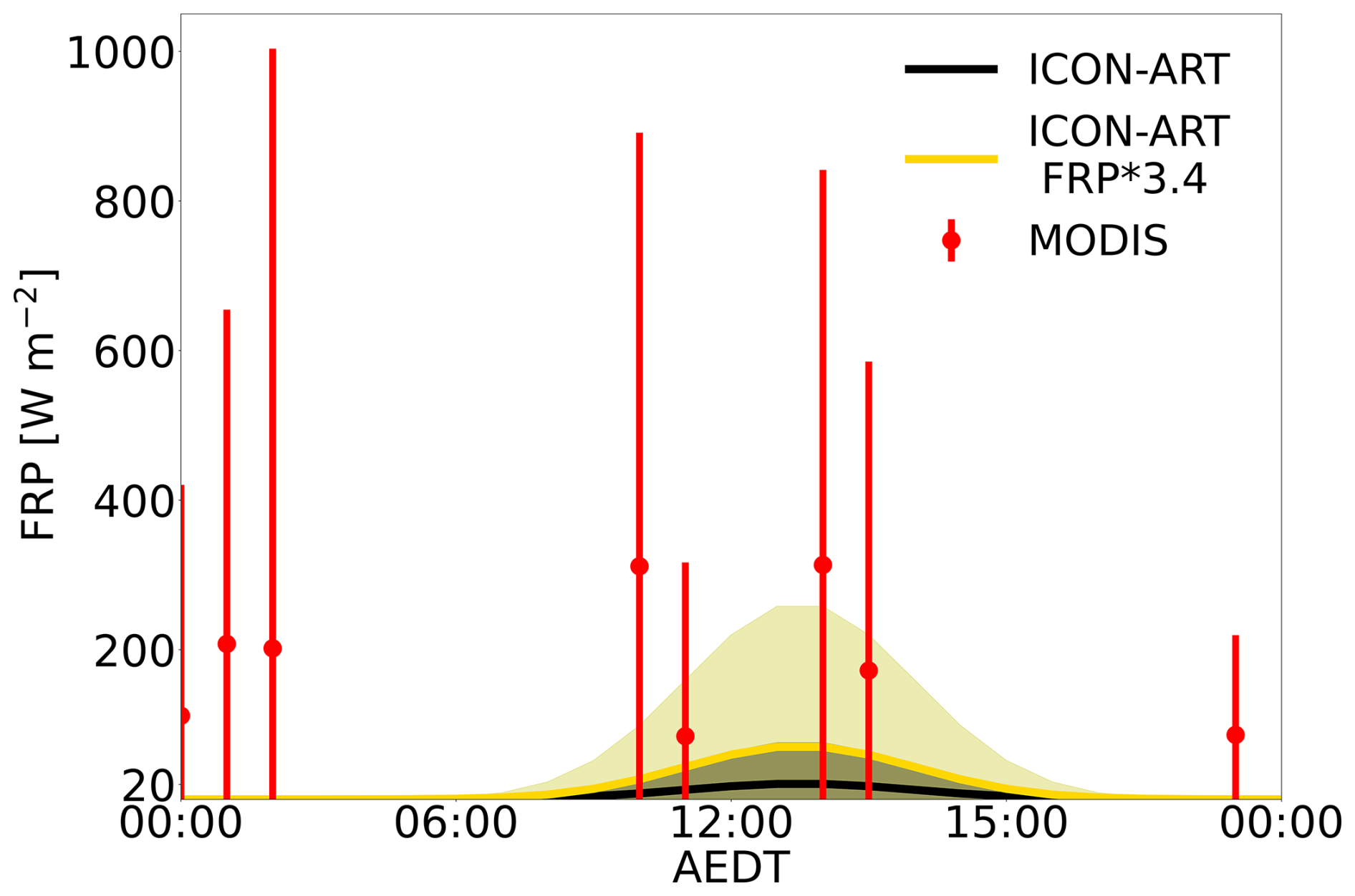
Figure A1 The averaged FRP assumed in the simulations (black line), and the standard deviation in gray without enhancement factor and FRP with 3.4 enhancement factor in yellow, with the standard deviation in dark yellow. Red dots represent the mean MODIS active FRP (NASA and University of Maryland, 2025) for each hour with measurements during the first simulation day (30 December 2029), along with the standard deviation.

Appendix B

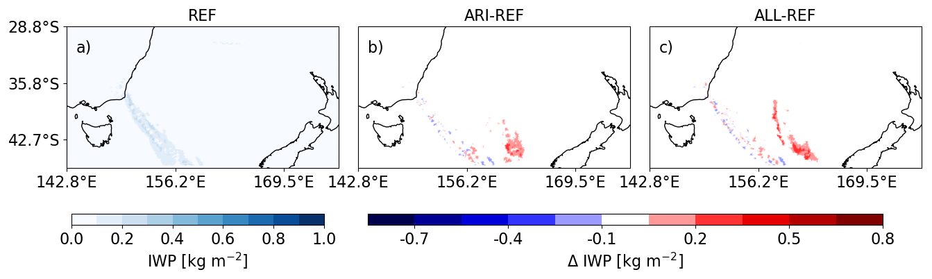
Figure B1 LWP for the (a) REF, difference in LWP for (b) ARI-REF, and (c) ALL-REF on 31 December at 14:30 AEDT.

Figure B2 IWP for the (a) REF, difference in IWP for (b) ARI-REF, and (c) ALL-REF on 31 December at 14:30 AEDT.

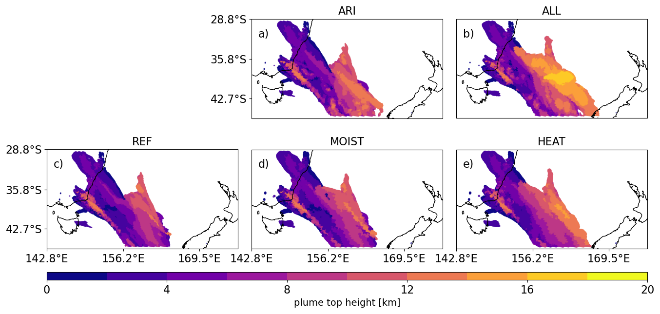
Figure B3 Plume top height for the (a) ARI, (b) ALL, (c) REF, (d) MOIST, (e) HEAT on 31 December at 14:30 AEDT.