Technical note: DACNO₂ – a multi-constraint deep learning framework for high-resolution 3D NO₂ field estimation

High-resolution 3D fields of nitrogen dioxide (NO₂) are critical for air quality management and satellite retrievals, yet traditional chemistry-transport models (CTMs) face challenges in fine-scale modeling. Machine learning (ML) alternatives often struggle with generalization and transferability, inheriting biases from CTMs or being limited by sparse surface measurements. We present the Deep Atmospheric Chemistry NO₂ model (DACNO₂), a deep learning model that generates daily 2 km × 2 km 3D NO₂ fields over Western Europe. The model's three-phase multi-constraint training strategy begins by pre-training on European Copernicus Atmosphere Monitoring Service (CAMS) reanalysis data to learn large-scale atmospheric patterns, then fine-tunes with CAMS and in-situ European Environmental Agency (EEA) surface data to correct biases and refine local detail, and completes with an adaptive fine-tuning to capture evolving trends. An evaluation for 2023 shows that DACNO₂ reproduces broad-scale 3D CAMS fields (R²=0.90) and improves agreement with independent EEA stations over the CAMS reanalysis (R² enhanced from 0.61 to 0.66; bias reduced from −1.15 to −0.38 µg m⁻³). The model resolves spatial details and exhibits physically plausible behavior. This hybrid training approach fuses the physical consistency of a process-based model with the real-world surface measurements, overcoming the limitations of using either constraint alone. Applying DACNO₂ a-priori profiles to TROPOMI retrievals increases tropospheric NO₂ columns by 3 % on average over those using European CAMS profiles, with enhanced contrast between low- and high-NO₂ regions, primarily attributable to improved resolution. These results demonstrate the framework's potential to advance air quality monitoring and satellite remote sensing.

1 Introduction

Nitrogen dioxide (NO₂) is a key atmospheric pollutant with significant impacts on air quality, human health, ecosystems, and atmospheric chemistry. Primary sources include traffic, industrial activities, and energy production, with additional contributions from natural emissions (Crippa et al., 2018). Accurate characterization of the spatiotemporal distribution of NO₂ is critical for both air pollution management and atmospheric chemistry research.

Chemistry Transport Models (CTMs) such as GEOS-Chem (Bey et al., 2001), TM5-MP (Krol et al., 2005; Williams et al., 2017; Huijnen et al., 2010), WRF-Chem (Grell et al., 2005), and the Copernicus Atmosphere Monitoring Service (CAMS) (Peuch et al., 2022; Inness et al., 2019) are widely used to simulate atmospheric NO₂ based on physical and chemical processes. However, most CTMs operate at coarse spatial resolution due to computational constraints and the limited availability of high-resolution emission inventories. This restricts their ability to represent fine-scale NO₂ variability and often results in spatial smoothing and underestimation, particularly in urban environments. Emission inventories are usually outdated and may omit localized and small-scale sources (Lu et al., 2025), contributing to uncertainties and discrepancies between bottom-up and top-down emission estimates (Kuik et al., 2018; Yang et al., 2021). While regional high-resolution CTMs are available, such as CAMS at 10 km × 10 km resolution (Douros et al., 2023; Ialongo et al., 2020) and regional WRF-Chem at 3 km × 3 km resolution (Kuhn et al., 2024b), challenges remain in accurately capturing urban and fine-scale NO₂ patterns (Meleux et al., 2024), and model optimization is often resource-intensive (Kuhn et al., 2024a, b).

CTM outputs also serve as a-priori NO₂ profiles for satellite retrievals (Palmer et al., 2001; Douros et al., 2023; Yang et al., 2023), supporting large-scale NO₂ monitoring. Over the past three decades, satellite NO₂ observations have been advancing toward higher spatiotemporal resolution. Satellite instruments such as the TROPOspheric Monitoring Instrument (TROPOMI, 7 km × 3.5 km, 5.5 km × 3.5 km since August 2019) on Sentinel-5P (Veefkind et al., 2012), the Geostationary Environment Monitoring Spectrometer (GEMS, 3.5 km × 8 km) (Kim et al., 2020), Tropospheric emissions: Monitoring of pollution (TEMPO, 2 km × 4.75 km) (Zoogman et al., 2017), Sentinel-4 (8 km × 8 km) (Gulde et al., 2017), Sentinel-5 (7.5 km × 7.5 km) (Bézy et al., 2014), Twin ANthropogenic Greenhouse Gas Observers (TANGO, 300 m × 300 m) (Landgraf et al., 2020), and the Copernicus Anthropogenic Carbon Dioxide Monitoring constellation (CO2M, 2 km × 2 km) (Sierk et al., 2021) are advancing spaceborne NO₂ observations to kilometer-scale resolution. This progress has increased demand for high-resolution a-priori profiles, which can better account for near-surface NO₂ enhancements and strong spatial gradients over emission hotspots in satellite NO₂ retrieval products. It motivates us to develop a 3D NO₂ product on a 2 km × 2 km horizontal grid (hereafter referred to as the 2 km grid) to better resolve fine-scale spatial heterogeneity and support the emerging high-resolution satellite missions (e.g., CO2M). However, CTM-based profiles remain constrained by the limitations mentioned above, highlighting the need for alternative modeling approaches.

Machine learning (ML) provides an efficient alternative for high-resolution NO₂ estimation. ML techniques have been widely applied for surface NO₂ mapping (Sun et al., 2024; Kim et al., 2021; Wei et al., 2022), and recent studies have extended these approaches for 3D NO₂ modeling above the surface. These studies have trained models on process-based 3D NO₂ fields generated by CTMs (Bodnar et al., 2024; Kuhn et al., 2024a), on vertical profiles from MAX-DOAS observations (Zhang et al., 2025; Zhang et al., 2022b; Jiang et al., 2025), and on a combination of process-based 3D NO₂ fields with satellite observations (Li and Xing, 2024). While these studies demonstrate the feasibility of ML-based 3D NO₂ modeling, challenges remain in achieving high spatial resolution, robust generalization, and transferability. Process-based data carries inherent biases and has relatively coarse resolution. Ground-based observations are sparse and unevenly distributed, limiting the model's spatial generalization. While Li and Xing (2024) combine process-based NO₂ fields with satellite NO₂ observations from the Ozone Monitoring Instrument (OMI) to train the ML model, the resulting product is still limited to a coarse resolution (27 km × 27 km).

In this study, we present the Deep Atmospheric Chemistry NO₂ model (DACNO₂), a deep learning model developed to produce daily, high-resolution 3D NO₂ fields on the 2 km grid with high accuracy, robust generalization, and transferability. DACNO₂ integrates multi-source inputs, including emissions, geography, meteorology, and temporal indicators. The model is trained using a phased, multi-constraint approach that combines process-based CAMS fields with ground-based EEA measurements. This method enables the model to reproduce broad-scale, process-based NO₂ patterns and capture local NO₂ gradients. The training strategy consists of three phases: pre-training, multi-constraint fine-tuning, and adaptive fine-tuning. Western Europe (5° W–9° E, 42–54° N) is chosen as the study region, given its diverse topography, high urbanization, and substantial industrial activity.

This study addresses two key research questions: (1) Can a deep learning framework combining multi-constraint and phased training overcome the resolution, bias, and generalization limitations of current CTM and ML approaches for 3D NO₂ modeling? (2) Does the DACNO₂ product on the 2 km grid improve fine-scale NO₂ representation to support applications in regional air quality management and satellite retrievals?

The remainder of this paper is organized as follows. Section 2 describes the DACNO₂ development framework, including dataset preparation, model architecture, and training strategy. Section 3 evaluates model performance. Section 4 discusses broader insights and implications. Conclusions and outlook are provided in Sect. 5.

2 Development Framework for DACNO₂

2.1 Framework Overview

DACNO₂ is developed to provide daily 3D NO₂ fields at high spatial resolution (2 km × 2 km) with improved accuracy and generalizability by integrating multi-source data, physically consistent process-based datasets, and real-world measurements. The overall framework, illustrated in Fig. 1, combines diverse data streams with a phased training strategy.

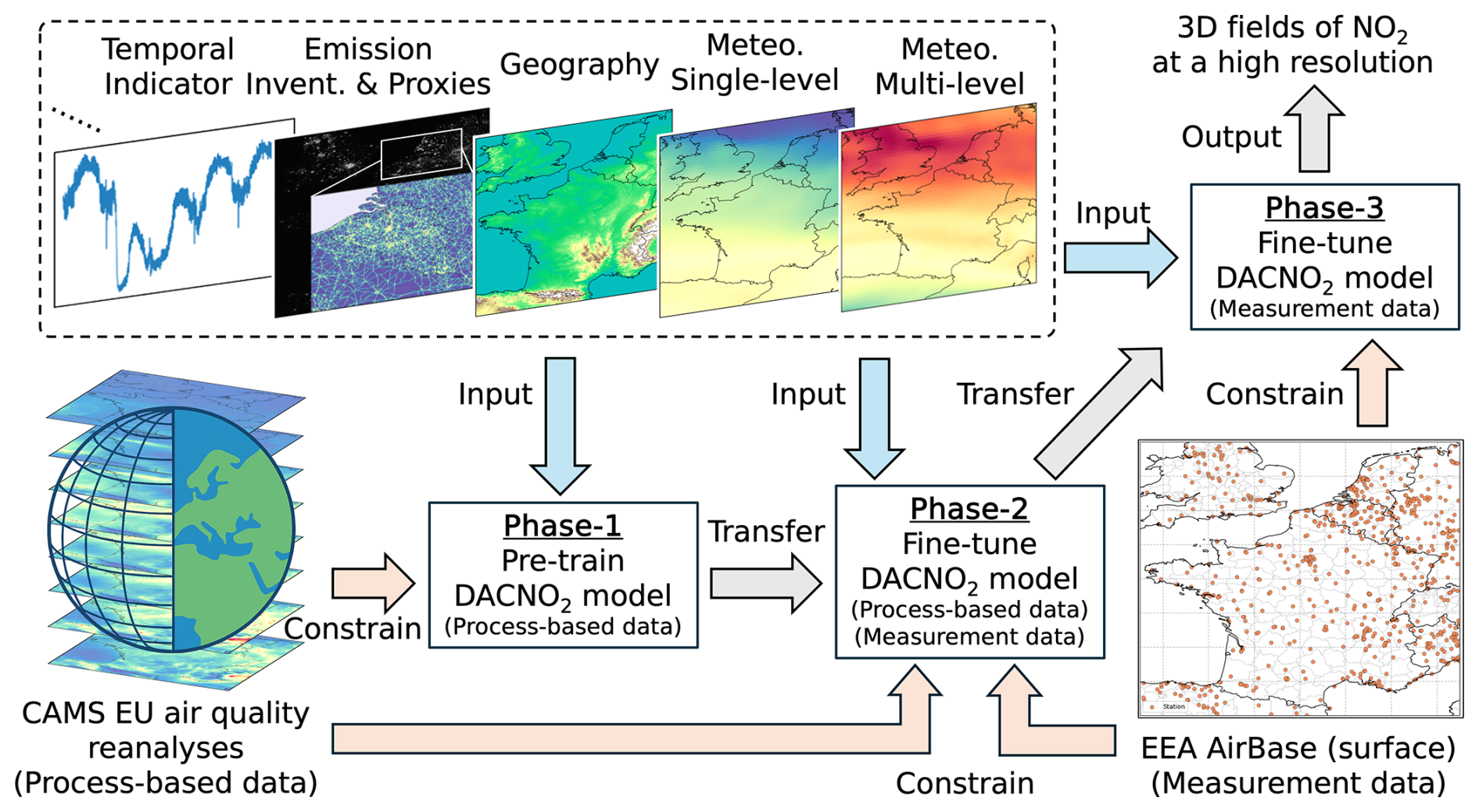
Figure 1 Overview of the DACNO₂ model development framework. The framework integrates multiple input data streams: temporal indicators, emission inventories and proxies, geography, and ERA5 meteorological data, with two target datasets: process-based NO₂ from CAMS European air quality reanalysis and ground-based in-situ EEA NO₂ measurements. The training is organized in three sequential phases: pre-training on process-based CAMS NO₂, multi-constraint fine-tuning with both CAMS and EEA data, and adaptive fine-tuning to recent NO₂ trends. The resulting model generates daily, high-resolution (2 km × 2 km) 3D NO₂ fields. Arrows indicate the data flow and phased training process.

DACNO₂ uses five groups of input features: temporal indicators, emission inventories and proxies, geographic data, ERA5 single-level meteorological variables, and ERA5 multi-level meteorological variables. Together, they provide complementary information on spatial and temporal NO₂ variability. For model training, the targets are process-based NO₂ fields from the CAMS European air quality reanalyses (Inness et al., 2019; Peuch et al., 2022) and real-world surface NO₂ measurements from the EEA AirBase network (European Environment Agency, 2024). CAMS supplies physically consistent large-scale 3D NO₂ distributions, while EEA data constrain the model to match local concentration patterns. Details on data preparation are provided in Sect. 2.2.

To effectively learn NO₂ patterns from diverse datasets, DACNO₂ employs an encoder–decoder architecture with five dedicated encoder branches, each tailored to a specific group of input features. The model structure is described in Sect. 2.3.

Model training is organized into three sequential phases. In Phase 1, a baseline model is pre-trained on process-based CAMS data. In Phase 2, the model is further trained with both process-based and measurement data, improving its ability to represent local NO₂ gradients. In Phase 3, the model is fine-tuned using recent measurements to reflect current NO₂ trends and support real-world applications. Details of the training approach are provided in Sect. 2.4.

2.2 Dataset Preparation

2.2.1 Input Features

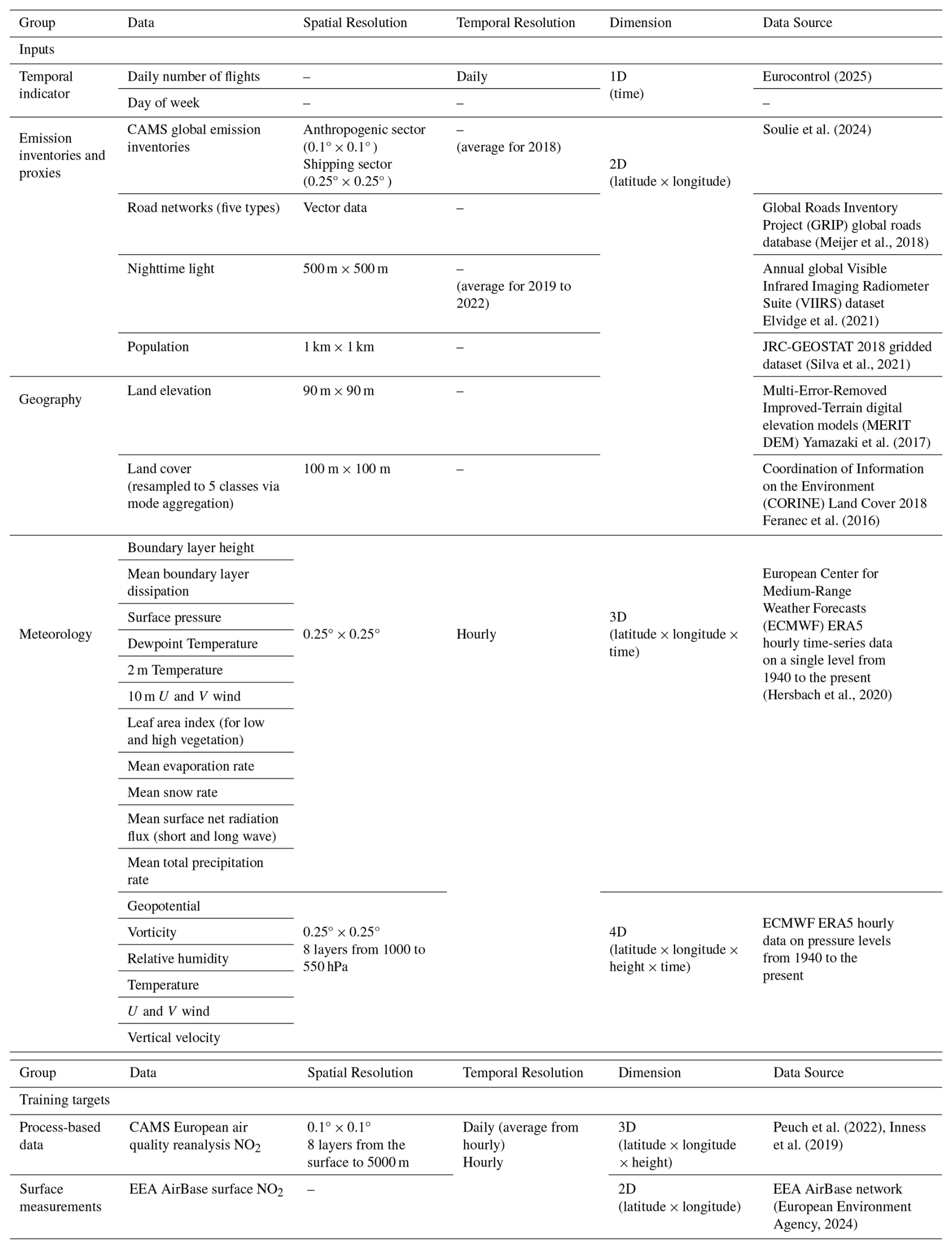
DACNO₂ utilizes 38 input datasets, organized into five groups: temporal indicators, emission inventories and proxies, geography, single-level meteorology, and multi-level meteorology. Details of all input features and their sources are provided in Table 1.

The temporal indicator group consists of the day of the week and the daily number of flights. The day of the week captures regular human activity cycles, reflecting variability between weekdays and weekends. Data on the daily number of flights, aggregated for nine countries in the study area (Eurocontrol, 2025), can indicate irregular activity such as holiday periods or major events, which may help explain the irregular changes in NO₂ emissions.

Emission inventories and proxies include anthropogenic NO_x emission inventories, road density, population density, and nighttime light. These features provide direct and indirect measures of NO_x emissions, with high-resolution proxies complementing inventories at finer spatial scales. All datasets are resampled to the 2 km grid using interpolation, averaging, or rasterization methods.

Geographic datasets include land elevation and land cover, providing terrain context to the ML model. Elevation influences atmospheric transport by creating physical barriers that can trap pollutants (Giovannini et al., 2020), while land cover serves as a proxy for the location and type of surface emissions (Beelen et al., 2013). Land cover is categorized into five classes: artificial surfaces, agricultural areas, forests and semi-natural areas, wetlands, and water bodies, aggregated from the original 44 categories by the mode method (the most frequently occurring land cover type). Both elevation and land cover data are resampled to the 2 km grid.

Meteorological features provide atmospheric information from the surface through the free troposphere, obtained from the European Centre for Medium-Range Weather Forecasts (ECMWF) ERA5 hourly single-level and multi-level (pressure-level) datasets (Hersbach et al., 2020). We use 24 h meteorological features for the target day. Meteorological data are horizontally resampled to the 16 km grid, for three reasons: (1) the native ERA5 resolution (0.25° × 0.25°, approximately 25 km × 25 km) is coarser than 2 km × 2 km, and bilinear interpolation would mainly introduce artificial smoothness rather than genuine fine-scale gradients; (2) retaining many meteorological variables at 2 km × 2 km would impose a significant computational burden; and (3) the DACNO₂ architecture uses a hierarchical encoder-decoder, where upscaling and downscaling follow a factor-of-two scaling scheme (e.g., 2, 4, 8, 16 km). Although the ERA5-Land data can provide higher resolution (0.1° × 0.1°, approximately 9 km × 9 km), it only covers the continental areas, which is inconsistent with the model application scope.

The day-of-week feature is normalized using sine and cosine transforms to retain its cyclical nature. Land cover is one-hot encoded to convert categorical data into a numerical format. All other input features are normalized with z-scores, based on the mean and standard deviation of the training set.

Notably, satellite-derived NO₂ products were deliberately excluded from the input features for two key reasons. First, frequent data gaps in satellite products, due to cloud cover and quality control, would propagate into the model's output, preventing the generation of continuous, gap-free fields. Second, this exclusion allows for an independent evaluation of the model against satellite observations and preserves the potential to use satellite data as an independent constraint in future work.

Table 1 Summary of inputs and training targets for the DACNO₂ model development.

2.2.2 Training Targets

The training targets include CAMS European air quality reanalysis profile data (CAMS NO₂) and in-situ measurements from the EEA AirBase network (EEA NO₂). The datasets are both listed in Table 1. CAMS NO₂ offers extensive and continuous 3D NO₂ data aligned with physical and chemical processes, while EEA NO₂ provides ground-based in-situ measurements from sparsely distributed monitoring stations.

CAMS NO₂ is the median ensemble of 11 different regional models (Inness et al., 2019; Peuch et al., 2022). The dataset provides hourly NO₂ distributions at eight vertical heights above the surface (surface, 50, 100, 250, 500, 750, 1000, 2000, 3000, and 5000 m) and has a horizontal resolution of 0.1° × 0.1° (10 km × 10 km). CAMS NO₂ has assimilated EEA observations and includes both interim and validated reanalyses. Interim data relies on near-real-time observations without full validation, whereas validated data undergo rigorous quality control with an additional delay. In this study, we used CAMS NO₂ data from 2019 to 2023, where the 2019–2021 data are validated reanalysis data and the 2022–2023 data are interim reanalysis data, based on data availability. CAMS NO₂ was processed by averaging hourly data to daily values and by bilinearly interpolating its horizontal resolution from 10 to 8 km to match the model's factor-of-two scaling scheme. This regridding is used for grid alignment only and supports the computation of the loss function during training. In addition, CAMS NO₂ concentrations at each vertical layer were rescaled by dividing them by the ratio of the mean NO₂ concentration at that layer to the mean surface-layer NO₂ concentration, where this ratio was calculated from the training dataset. This adjustment ensures that the model gives adequate attention to higher-altitude NO₂ concentrations, which are otherwise much lower than surface values and could be neglected during training (Li and Xing, 2024; Kuhn et al., 2024a). During model inference, the predicted NO₂ concentrations at each layer were multiplied by the corresponding ratio to restore the original vertical profile.

EEA NO₂ was collected from background and industrial monitoring stations (European Environment Agency, 2024) and mapped onto the 2 km grid. Such stations have spatial representativeness of several to dozens of square kilometers, enabling cover our target grid size. However, traffic stations were excluded because their measurements represent a very local area (< 1 km²), significantly smaller than the 2 km grid cells of our study (Kracht et al., 2017). If multiple stations were located within the same grid cell, their values were averaged. When both background and industrial stations existed in a grid cell, the cell was classified as background. The stations with at least 20 % effective observations per year are selected. In total, 748 grid cells with measurements were identified, with 575 assigned for training and 173 for final evaluation. Because background EEA NO₂ is assimilated into CAMS, the split of background stations followed the CAMS model assimilation system (Copernicus Atmosphere Monitoring Service, 2024) to prevent data leakage, while industrial stations were randomly split. All EEA NO₂ data were converted from hourly to daily averages. The spatial distribution of training and evaluation stations is shown in Fig. S1 in the Supplement, along with the distribution density and the average surface NO₂ concentration map. It is important to note that some in-situ NO₂ measurements can be biased positively. This occurs because chemiluminescence instruments equipped with heated molybdenum converters can partially convert other reactive nitrogen species (NO_z, such as peroxyacetyl nitrate (PAN) and HNO₃) and misreport them as NO₂. This introduces an NO_y bias into the EEA measurements (Lamsal et al., 2008; Villena et al., 2012). To address this issue in future research, one potential approach is to use chemical model simulations, such as WRF-Chem, to estimate this interference and adjust the affected monitoring stations (Kuhn et al., 2024a).

2.2.3 Patch-Based Data Processing and Reconstruction

To balance the model's receptive field and computational efficiency, we used a patching method because training and inference on the full domain on the 2 km grid as a single sample is not feasible, given the multi-branch 2D and 3D inputs and the 3D decoder. Specifically, all datasets except the temporal indicator were divided into patches of 512 km × 512 km with partial overlap. This produced grid sizes of 32 × 32 for ERA5 meteorological data, 64 × 64 for CAMS NO₂ data, and 256 × 256 for emission inventories and proxies, geographic data, and EEA NO₂ data. The patch size retains regional spatial context relevant for NO₂ variability while remaining compatible with the factor-of-two scaling scheme used in the encoder–decoder. Partial overlapping is used to reduce boundary effects because predictions near patch edges have reduced spatial context, and overlapping patches ensure each grid cell is predicted from at least one patch interior. In this study, each patch was treated as a single input sample, and the stride was set to generate 12 overlapping samples per day, covering the full domain while keeping the daily sample count computationally manageable. More samples can be generated as needed by reducing the stride of the sliding window. Additionally, if targeting higher resolution (e.g., 1 km × 1 km or 500 m × 500 m), larger patches are required, resulting in an exponential increase in computational cost.

During model inference, the output patches were merged using a weighted averaging scheme based on a 2D Hann window (Oppenheim, 1999), which assigns lower weights to patch edges and higher weights to central regions. For each grid cell, weighted values from all overlapping patches were summed and normalized by the total weights. This reconstruction method reduced edge artifacts in overlapping areas and ensured smooth transitions across patch boundaries.

2.3 Model Architecture and Design

The architecture of the DACNO₂ model is illustrated in Fig. 2. The model adopts an encoder–decoder framework with residual connections (He et al., 2016) to map multi-source input features to the daily 3D NO₂ field. The residual connections pass intermediate feature maps from the encoder directly to matching decoder stages, which helps retain fine-scale information across the upscaling path and improves training stability. DACNO₂ integrates several types of neural network modules, including multilayer perceptron (MLP), convolutional neural network (CNN), and convolutional long short-term memory (ConvLSTM), to process and fuse heterogeneous input tensors. Each module is chosen for its specific strengths in handling different data structures. ConvLSTM is for spatiotemporal sequences, CNN is for spatial hierarchies, and MLP is for tabular feature vectors. Inception-style structures are applied in several neural network modules to enable the model to capture both local-scale and broader-scale spatial features.

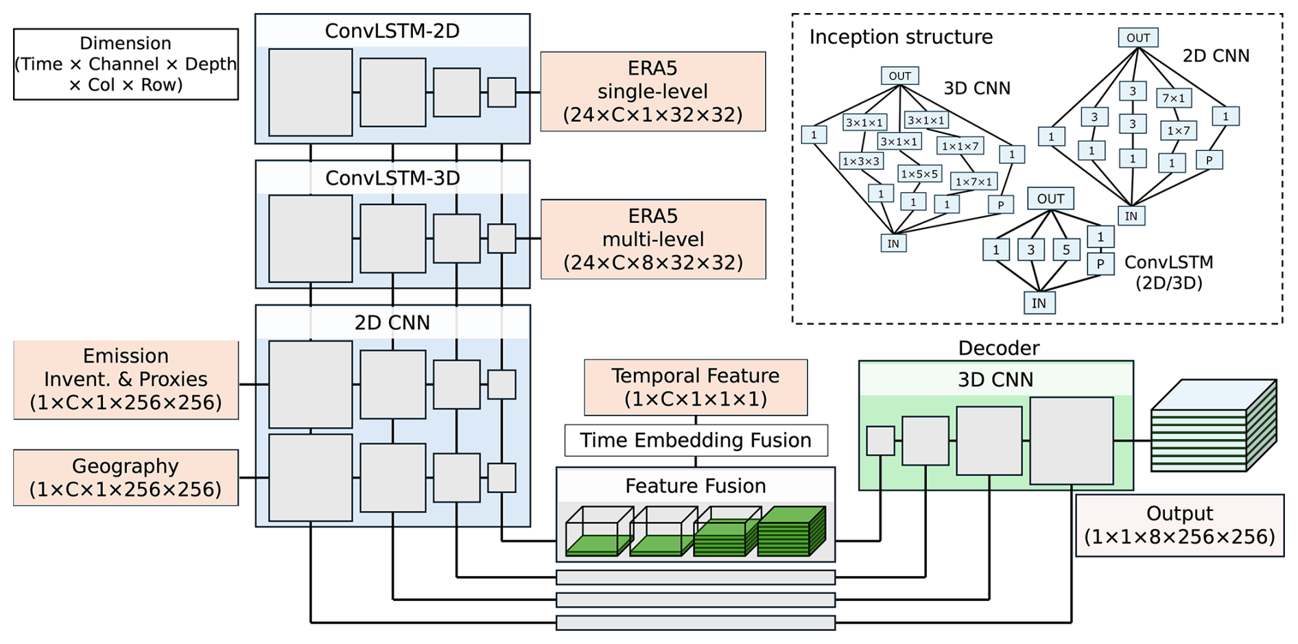
Figure 2 DACNO₂ model architecture. The model features a multi-branch encoder–decoder design for daily 3D NO₂ prediction. Five input groups are processed separately: ERA5 single-level meteorological variables (ConvLSTM-2D), ERA5 multi-level meteorological variables (ConvLSTM-3D), emission inventories and proxies (2D CNN), geography (2D CNN), and temporal features (MLP-based embedding fusion). Outputs from all encoder branches are fused and passed into a unified 3D CNN decoder to generate high-resolution NO₂ fields. The architecture enables the extraction of spatial, temporal, and multi-level atmospheric features, supporting fine-scale NO₂ modeling. Input and output dimensions are indicated for each module.

2.3.1 Encoder and Decoder

DACNO₂ encodes ERA5 single-level (hourly 2D) and multi-level (hourly 3D) meteorological data using ConvLSTM-2D and ConvLSTM-3D modules, respectively. Both modules are based on the ConvLSTM architecture proposed by Shi et al. (2015), which combines convolutional layers for spatial feature extraction with long short-term memory (LSTM) units for temporal sequence modeling. LSTM units use gated memory to retain information from earlier time steps (Hochreiter and Schmidhuber, 1997), so the ConvLSTM branches can learn day-scale meteorological evolution rather than treating each hour independently. ERA5 data are processed using a progressive upscaling strategy, where the horizontal grid size increases stepwise from 32 × 32 to 64 × 64, 128 × 128, and 256 × 256, while the vertical dimension remains at 8 for multi-level inputs. This upscaling preserves spatial detail and enables residual connections to the decoder, unlike conventional encoders that downsample feature maps. To manage computational cost, the temporal sequence length is halved after each ConvLSTM block through subsampling, resulting in sequence lengths of 24, 12, 6, and 3 at successive stages. At each stage, the last time slice is extracted for feature fusion.

Emission and geographic variables are encoded by dedicated 2D CNN blocks, which extract hierarchical spatial features as the resolution decreases from 256 × 256 to 32 × 32. At the 32 × 32 latent stage, features from all four branches are passed through CNN-based transition layers, each forming a 3D tensor. The latent space represents a compressed internal representation where all encoder branches are mapped onto a common 3D tensor before the decoder reconstructs the 2 km × 2 km output fields. For each branch, feature values are assigned only to physically relevant vertical layers within the tensor, while all other layers are set to zero. Specifically, emission and geographic features are assigned to the surface layer, ERA5 single-level features are placed in the lowest five layers, and ERA5 multi-level features span all vertical layers. The resulting tensors are concatenated along the channel dimension and fused using a 3D CNN block. Temporal indicators are encoded by an MLP, then expanded to match the latent spatial dimensions, and integrated at this stage, allowing the model to capture both spatial and temporal context. The same feature fusion scheme is applied to residual connections between the encoder and decoder across multiple spatial scales, although temporal embedding is used only at the 32 × 32 stage.

The decoder uses 3D CNN modules with hierarchical upscaling from 32 × 32 to 256 × 256 in the horizontal dimension, while maintaining a vertical size of 8. This structure learns spatial correlations across multiple altitude layers and captures both horizontal and vertical dependencies in NO₂ distributions. All 2D and 3D CNN blocks use the sigmoid linear unit (SiLU) activation function (Elfwing et al., 2017), while the output layer uses the softplus activation function to ensure non-negative estimates of the 3D NO₂ field.

2.3.2 Inception-Based Modules

To enhance multi-scale feature extraction, DACNO₂ incorporates inception modules throughout its architecture (Fig. 2), inspired by the work of inception architecture (Szegedy et al., 2014, 2015). Each inception module runs multiple convolutional paths with different kernel sizes in parallel and concatenates their outputs, so DACNO₂ can capture both local gradients and broader regional structure within the same layer. In the ConvLSTM-2D and ConvLSTM-3D branches, each inception block applies parallel convolutional operations with varying kernel sizes (1 × 1, 3 × 3, 5 × 5) and a max-pooling branch, enabling the model to capture both local and broader spatiotemporal patterns. The max-pooling branch performs spatial downsampling by taking local maxima, which provides a coarse-scale summary that complements the convolution branches and improves multi-scale feature extraction. The 2D CNN modules extend this approach, combining parallel 1 × 1, 3 × 3, and 5 × 5 convolutions, a factorized 7 × 7 path (decomposed into 1 × 7 and 7 × 1 convolutions), and a pooling branch. For 3D CNN modules, inception blocks use parallel convolutions with different spatial and vertical kernel shapes, such as 1 × 1 × 1, 1 × 3 × 3, and 3 × 1 × 1, along with a pooling branch. In all cases, each parallel branch includes its own batch normalization, activation, and dropout, after which the outputs are concatenated along the channel dimension. Batch normalization normalizes intermediate activations within each mini-batch, reducing sensitivity to feature scaling and often improving optimization behavior (Ioffe and Szegedy, 2015). Dropout randomly masks a fraction of activations during training, which reduces overfitting and helps generalization when training on heterogeneous inputs (Srivastava et al., 2014). A similar design has been applied in a previous deep learning model for NO₂ estimation (Zhang et al., 2022a). It enables the model to effectively integrate information across multiple spatial and vertical scales, improving the representation of complex atmospheric NO₂ distributions.

2.4 Three-Phase Training Strategy

The DACNO₂ model development employs a three-phase training strategy, including pre-training, multi-constraint fine-tuning, and adaptive fine-tuning. Such a strategy enables the model to learn general patterns (e.g., a-priori knowledge) from a broad dataset and then transfer this internal knowledge to improve its performance on a new, more specific task. Similar approaches have been widely adopted in the development of artificial intelligence (AI) models across various domains, such as earth system modeling, large language models, and biomedical image analysis (Zhuang et al., 2019; Zhou et al., 2017; Ding et al., 2023; Bodnar et al., 2024).

2.4.1 Phase-1

In the first phase, the DACNO₂ model was pre-trained on the CAMS NO₂ data. This dataset provides physically consistent 3D NO₂ distributions by assimilating real-world observations into chemical transport models (Inness et al., 2019), enabling the model to learn comprehensive 3D NO₂ patterns governed by broad-scale atmospheric processes. This approach is inspired by recent progress in AI weather modeling (Bi et al., 2023; Lam et al., 2023) and the earth system foundation model (Bodnar et al., 2025), which uses ERA5 and CAMS data for 3D forecasting of weather and air quality.

In this step, the training loss is defined as the sum of the Mean Squared Error (MSE) loss and the Structural Similarity Index Measure (SSIM) loss (Zhao et al., 2017; Zhou et al., 2004) between the DACNO₂ prediction and the CAMS NO₂ data on the 8 km grid.

$$\begin{array}{}\text{(1)}& \begin{array}{rl}\mathrm{Loss}& ={\mathrm{LossMSE}}_{{\mathrm{DACNO}}_{\mathrm{2}}-\mathrm{CAMS}}\\ & +{\mathrm{LossSSIM}}_{{\mathrm{DACNO}}_{\mathrm{2}}-\mathrm{CAMS}}\end{array}\end{array}$$

MSE quantifies the absolute differences in NO₂ concentrations, while SSIM evaluates the similarity of spatial patterns between model outputs and the CAMS reference. SSIM is computed independently at each vertical layer by comparing normalized 2D horizontal slices of the predicted and reference NO₂ fields. Specifically, each slice is min-max normalized to the range of 0 to 1 prior to SSIM calculation, ensuring that the SSIM loss reflects only structural similarity rather than magnitude differences. The final SSIM loss is calculated as one minus the mean SSIM across all vertical layers. This dual-loss formulation encourages the model to match both the overall concentration values and the spatial structures of 3D NO₂ fields.

The model was trained and validated using a random sample split from the 2019, 2021, and 2022 datasets (13 140 samples, 80 % for training, 20 % for validation), with 2023 reserved as an independent test set. Data from 2020 was excluded from this process because a preliminary experiment showed that its inclusion substantially degraded the model performance on the unknown period (i.e., 2022 data, which was initially held out as an independent validation year in that experiment). This might be due to the unexpectedly higher NO₂ concentrations above 1000 m in that year (Fig. S2), which is also documented in the CAMS Evaluation and Quality Control (EQC) report (Meleux et al., 2023). While the cause remains unclear, we speculate that this anomaly is related to the substantial decrease in NO_x emissions during 2020 due to the COVID-19 pandemic (Levelt et al., 2022) and not well accounted for in the CAMS model. We evaluate and discuss DACNO₂ performance for that special year in Sect. 4.4.

2.4.2 Phase-2

In the second phase, we fine-tuned DACNO₂-Phase-1 by introducing an additional MSE constraint based on EEA NO₂, while maintaining the CAMS NO₂ constraints, as shown in Eq. (2). The EEA NO₂ MSE was computed at the surface layer and only on the 2 km grid with available EEA data

$$\begin{array}{}\text{(2)}& \begin{array}{rl}\mathrm{Loss}& ={\mathrm{LossMSE}}_{{\mathrm{DACNO}}_{\mathrm{2}}-\mathrm{CAMS}}\\ & +{\mathrm{LossSSIM}}_{{\mathrm{DACNO}}_{\mathrm{2}}-\mathrm{CAMS}}\\ & +{\mathrm{LossMSE}}_{{\mathrm{DACNO}}_{\mathrm{2}}-\mathrm{EEA}}\end{array}\end{array}$$

The EEA NO₂ data were split into training and evaluation sets using the same spatiotemporal alignment as the CAMS NO₂ split. Most training settings remained consistent with the first phase, except that the learning rate was reduced and the EEA NO₂ MSE term was added to both the training loss and the validation metric. The model checkpoint with the best validation performance was selected and is referred to as DACNO₂-Phase-2 for subsequent use. Although Phase-2 includes the same CAMS constraint as Phase-1, which may make Phase-1 appear redundant, we recommend retaining Phase-1. Skipping directly to Phase-2 can cause the model to overfit local EEA observations and limit its ability to learn generalizable NO₂ patterns from process-based data.

2.4.3 Phase-3

Recent changes in air quality policies and emission technologies (Castellanos and Boersma, 2012; Wang et al., 2021; Chang et al., 2023) may introduce systematic NO₂ variations that are not well represented in the historical training dataset (Fig. S7). To ensure the DACNO₂ model remains adaptable to such real-world changes, we introduced a third phase. In this step, we adopted a strategy inspired by the data assimilation system in the CAMS model (Inness et al., 2019). DACNO₂-Phase-3 is initialized from the DACNO₂-Phase-2 weights and further fine-tuned using EEA NO₂ data from the training stations during the test period (2023 in this study) to reflect a typical application scenario. To maintain spatial patterns learned from earlier phases, a regularization term based on SSIM was added to both the training loss and validation metric. SSIM was computed at 8 km × 8 km resolution between predictions from the updated model and DACNO₂-Phase-2 (Eq. 3):

$$\begin{array}{}\text{(3)}& \begin{array}{rl}\mathrm{Loss}& ={\mathrm{LossMSE}}_{{\mathrm{DACNO}}_{\mathrm{2}}\left(\mathrm{new}\right)-\mathrm{EEA}}\\ & +{\mathrm{LossSSIM}}_{{\mathrm{DACNO}}_{\mathrm{2}}\left(\mathrm{new}\right)-{\mathrm{DACNO}}_{\mathrm{2}}(\mathrm{Phase}-\mathrm{2})}\end{array}\end{array}$$

This approach allows the updated model to adjust prediction magnitudes in response to new measurements while preserving spatial patterns established in previous phases, since the CAMS constraint is no longer available in Phase-3. The model checkpoint with the best validation performance was selected and is referred to as DACNO₂-Phase-3, which incorporates recent real-world NO₂ variations while retaining consistency with patterns learned during earlier training.

2.4.4 Training and Implementation

DACNO₂ was trained and implemented in Python using PyTorch on two NVIDIA A30 GPUs. Training was performed with a batch size of 56, achieved by gradient accumulation. The first and second training phases each required approximately three weeks to complete 200 epochs on three years of data. The third training phase required about one week for 100 epochs on a single year of data. Once trained, the model generates daily NO₂ estimates for the whole area within minutes. Further efficiency improvements are possible through hardware upgrades or model optimization.

3 Assessing DACNO₂ Performance and Evolution

3.1 Model Performance Across Training Phases

The performance of the DACNO₂ model was evaluated using both EEA NO₂ and CAMS NO₂ test data from 2023. For the comparison against EEA NO₂ (results in the upper panel of Table 2), both DACNO₂ outputs and CAMS NO₂ were evaluated on the 2 km grid. The CAMS NO₂ data was interpolated to 2 km × 2 km resolution (CAMS-2km) and served as the baseline for this comparison. The performance results were calculated across all paired measurements and model estimations. The station-specific time-series consistency analyses are provided in Fig. S3, where the results for each EEA evaluation station were calculated along the daily time-series independently. The average time-series consistency between models and EEA NO₂ is shown in Fig. S4. For the evaluation of DACNO₂ using CAMS NO₂ (results in the lower panel of Table 2), DACNO₂ outputs were evaluated at the CAMS original 10 km × 10 km resolution across all vertical layers, as well as for individual layers. The layer-wise temporal correlations at the regional average and grid scales are illustrated in Fig. S6. Evaluation metrics included the root mean squared error (RMSE), Pearson correlation coefficient (r), coefficient of determination (R²), and bias.

Table 2 Performance of DACNO₂ on the 2023 test dataset.

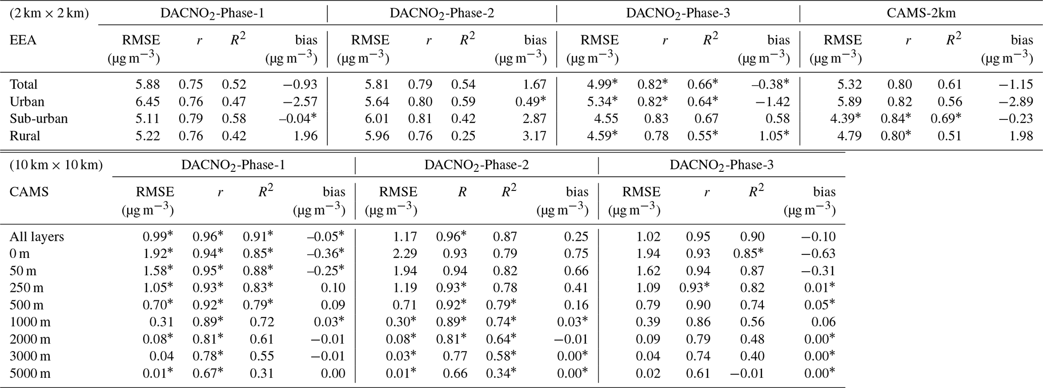
Note: For the comparison against EEA NO₂ (shown in the upper panel), both DACNO₂ outputs and CAMS NO₂ were evaluated on the 2 km grid. In this comparison, CAMS is a reanalysis product that has assimilated EEA NO₂ for 2023. The CAMS NO₂ data was interpolated to a 2 km × 2 km resolution (CAMS-2km) and used as a baseline in this comparison. For evaluating DACNO₂ using CAMS NO₂ (shown in the lower panel), DACNO₂ outputs were downsampled and evaluated at the original 10 km × 10 km resolution of CAMS across all vertical layers as well as for individual layers. Best values within each row are marked with an asterisk (^*).

Phases 1–3 represent successive development stages of the DACNO₂ model. The phase-to-phase comparison in Table 2 is used to quantify the incremental effect of adding constraints and the final adaptation step. In Phase-3, the fine-tuning step uses EEA observations from the training stations in 2023. All reported EEA-based metrics are computed on the held-out evaluation stations. Comparisons with EEA NO₂ indicate progressive improvement across DACNO₂ training phases. DACNO₂-Phase-3 achieves the best overall agreement (RMSE = 4.99 µg m⁻³, r=0.82, R²=0.66, bias = −0.38 µg m⁻³), outperforming both DACNO₂-Phase-1 (RMSE = 5.88 µg m⁻³,r=0.75, R²= 0.52, bias = −0.93 µg m⁻³) and DACNO₂-Phase-2 (RMSE = 5.81 µg m⁻³, r=0.79, R²=0.54, bias = 1.67 µg m⁻³). Figure S4 shows that the DACNO₂ model learns reliable temporal correlations with EEA NO₂ at the daily and seasonal scales since Phase-1 (r=0.94), and these correlations are further enhanced in Phase-2 (r=0.95) and Phase-3 (r=0.98). This indicates that the model can represent temporal variability without using satellite NO₂ as an input, relying instead on meteorological and temporal indicators. Moreover, Table 2 and Fig. S4 show a positive bias for DACNO₂-Phase-2 in 2023. This offset is consistent with the fact that the NO₂ level in 2023 is lower than in the Phase-2 training years (2019, 2021, 2022), as illustrated in Fig. S7. DACNO₂-Phase-3 reduces the effect of the interannual variation while maintaining the temporal correlation, highlighting the role of the adaptive fine-tuning step.

Compared to the interpolated CAMS-2km dataset (RMSE = 5.32 µg m⁻³, r=0.80, R²=0.61, bias = −1.15 µg m⁻³), DACNO₂-Phase-3 shows improved accuracy and reduced bias. Station-type analysis further highlights the advantages of DACNO₂-Phase-3, especially at urban and rural sites. For urban locations, DACNO₂-Phase-3 achieves better agreement (RMSE = 5.34 µg m⁻³, r=0.82, R²=0.64, bias = −1.42 µg m⁻³) compared with CAMS-2km (RMSE = 5.89 µg m⁻³, r=0.82, R²=0.56, bias = −2.89 µg m⁻³). In rural areas, DACNO₂-Phase-3 reduces the bias (RMSE = 4.59 µg m⁻³, bias = 1.05 µg m⁻³) compared to CAMS-2km (RMSE = 4.79 µg m⁻³, bias = 1.98 µg m⁻³). Such improvement is consistent with station-specific time-series consistency analysis (Fig. S3). It indicates that DACNO₂-Phase-3 achieves station-specific Pearson correlations comparable to CAMS-2km (CAMS-2km: r-mean = 0.85, r-median = 0.88; DACNO₂-Phase-3: r-mean = 0.84, r-median = 0.87), while exhibiting higher station-specific R² (CAMS-2km: R²-mean = 0.09, R²-median = 0.52; DACNO₂-Phase-3: R²-mean = 0.23, R²-median = 0.61). The R² improvements are attributed to more high-R² sites at urban stations and fewer very low-R² sites at rural stations. The large difference between the mean and median R² is primarily caused by negative R² values at a subset of rural stations, likely due to uneven station distribution across the network and the challenge of modeling weaker, noisier signals in rural environments. Overall, these results suggest that the DACNO₂ model improves agreement with the independent EEA evaluation stations relative to the CAMS-2km baseline across station types. The associated spatial redistribution and localized patterns are examined explicitly in Sect. 3.2.

In addition, Fig. S3 shows that DACNO₂-Phase-3 achieves better station-specific agreement in the central domain than near the boundaries. This may be due to boundary areas that lack sufficient spatial context and have complex mountainous terrain. Additionally, a slight overestimation of DACNO₂-Phase-3 at EEA rural stations persists despite adaptive fine-tuning. A possible reason is the imbalance in the EEA constraint. Figure S1 shows that most stations are located in urban and suburban areas with relatively higher NO₂ concentrations, whereas fewer stations are in rural areas. This may lead to positive bias in the model's estimates for rural areas, and the solutions require further investigation, including sample rebalancing strategies, expanding the study region to include more rural sites, and additional constraints. Meanwhile, given the R² definition, positive prediction bias at rural stations may be influential, as these stations generally have low NO₂ standard deviations and a smaller tolerance for prediction bias.

Comparisons with CAMS NO₂ across all layers show that DACNO₂ effectively learns and preserves 3D NO₂ distributions through all training phases (Table 2). Figure S6 further presents a layer-wise comparison between DACNO₂-Phase-3 and CAMS at the temporal and grid scales, showing that DACNO₂-Phase-3 can capture the temporal variability of NO₂ in 3D space. Near the surface, DACNO₂-Phase-3 maintains strong agreement with CAMS (Layer 0 m: RMSE = 1.94 µg m⁻³, r = 0.93, R²=0.85, bias = −0.63 µg m⁻³, Table 2), and performance remains robust at mid-altitudes (Layer 500 m: RMSE = 0.79 µg m⁻³, r = 0.90, R²=0.74, bias = 0.05 µg m⁻³), similar to earlier phases. However, a weak correlation is observed in the mountainous region (i.e., the Alps and the Pyrenees, Fig. S6). At higher layers above 1000 m, the agreement in R² starts to decrease while the correlation remains stable. At 5000 m, DACNO₂-Phase-3 yields a near-zero R² (−0.01), which is lower than DACNO₂-Phase-1 (0.31) and DACNO₂-Phase-2 (0.34), but the correlation remains moderate (r≥0.6). Figure S6 indicates that the differences between DACNO₂-phase-3 and CAMS at these higher layers are mainly due to magnitude adjustment rather than loss of spatial structure. In addition, predicting very low NO₂ concentrations (approximately 0.05 µg m⁻³ at 3000 m and 0.02 µg m⁻³ at 5000 m, Fig. S2) at high layers is challenged by relatively higher noise. This reduction in agreement at upper layers remains a key challenge for ML-based 3D air quality modeling, which may require additional constraints from space-based observations or physical processes.

3.2 Model Evolution in the Multi-constraint Strategy

To further illustrate the evolution of estimated NO₂ spatial distributions achieved through a phased training, multi-constraint strategy, Fig. 3 compares average surface NO₂ estimates for 2023 from DACNO₂-Phase-1, DACNO₂-Phase-2, DACNO₂-Phase-3, CAMS, and CAMS-2km. Results are shown for the full study region and three representative local areas of Paris, the northern region (NO₂ hotspot area encompassing the Netherlands, Belgium, and the Ruhr area), and the Alpine region.

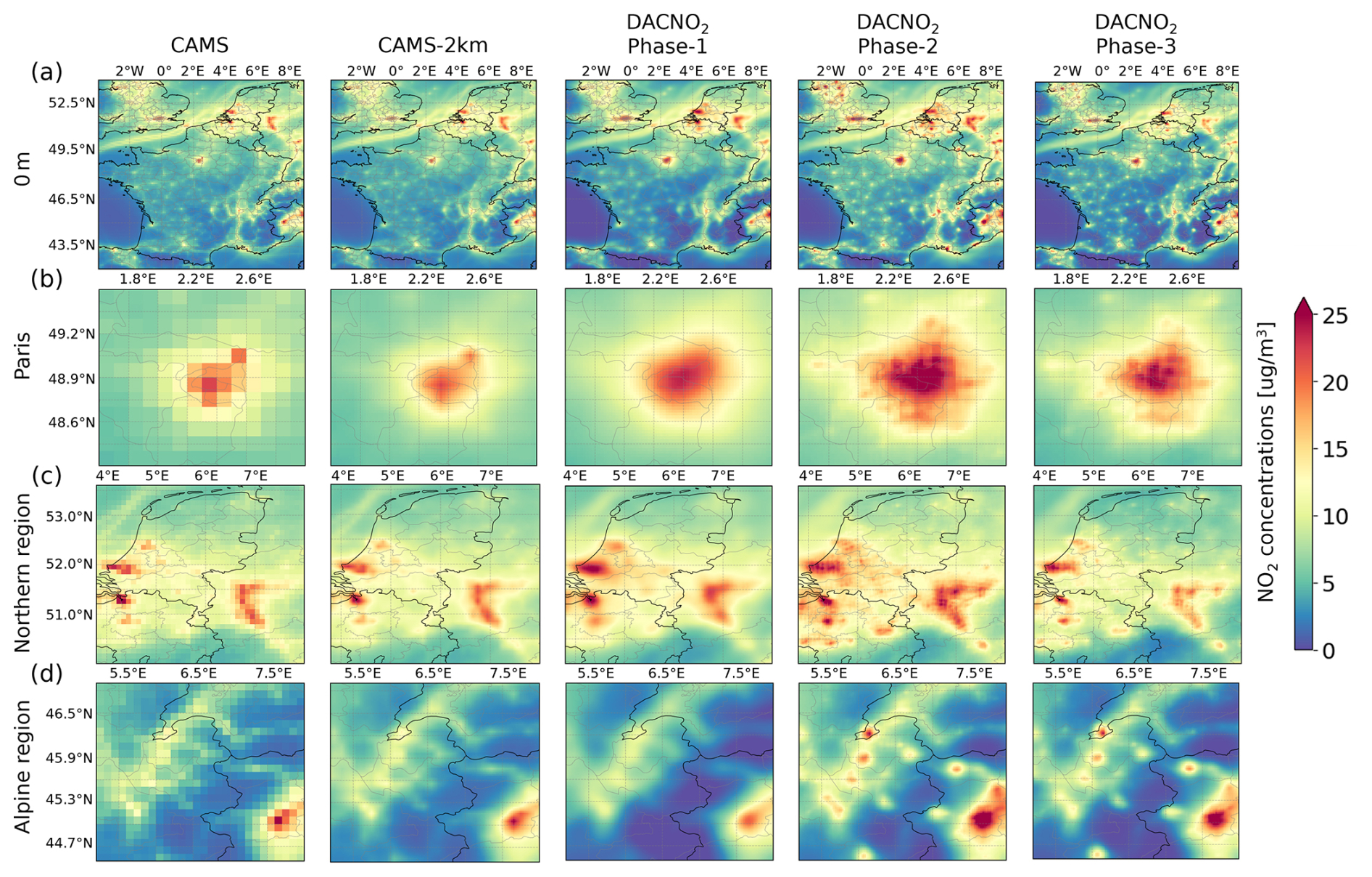
Figure 3 Spatial comparison of surface NO₂ estimates for 2023 from multiple models. (a) Annual mean surface NO₂ fields over the entire study region from DACNO₂-Phase-1, DACNO₂-Phase-2, DACNO₂-Phase-3, CAMS (10 km × 10 km), and CAMS-2km (bilinearly interpolated to 2 km × 2 km). (b–d) Enlarged views for three representative local areas: (b) Paris, (c) the northern region (NO₂ hotspot area encompassing the Netherlands, Belgium, and the Ruhr area), and (d) the Alpine region.

Across the study region (Fig. 3a), all models exhibit broad and similar NO₂ patterns over land and ocean, consistent with the high spatial agreement between DACNO₂ and CAMS NO₂ reported in Sect. 3.1. Nonetheless, DACNO₂-Phase-2 and DACNO₂-Phase-3 yield sharper spatial contrasts and more clearly defined local NO₂ hotspots than CAMS and DACNO₂-Phase-1. As an additional experiment, we trained the model using only EEA NO₂ data, resulting in the DACNO₂-onlyobs version. As shown in Fig. S8, this model yields effective NO₂ estimates primarily limited to the land surface and cannot reproduce the shipping track patterns, which are visible in the CAMS and DACNO₂ results. Meanwhile, this model produces obvious artifacts over the ocean and at higher altitudes due to the lack of training constraints. These differences highlight the significance of the CAMS NO₂ constraint in facilitating broad spatial generalization in ML-based models.

Differences between models become more pronounced when focusing on local regions (Fig. 3b–d). CAMS NO₂ exhibits visible pixelation effects in these areas due to its coarse native resolution. While bilinear interpolation (as in CAMS-2km) can smooth these effects, it does not introduce additional spatial detail, resulting in oversmoothed patterns. DACNO₂-Phase-1 shows a spatial NO₂ distribution similar to CAMS-2km, despite using high-resolution input features from emission proxies and geography. This indicates that constraints from CAMS NO₂ alone are insufficient for the model to capture fine-scale local NO₂ variability. Incorporating the EEA NO₂ constraint in DACNO₂-Phase-2 addresses this limitation, inspired by approaches in recent ML-based high-resolution surface NO₂ modeling studies using ground measurements as targets (Sun et al., 2024; Wei et al., 2022; Kim et al., 2021; Ghahremanloo et al., 2023). DACNO₂-Phase-2 reconstructs spatial patterns of NO₂ that better match urban layout in Paris (Fig. 3b), identifies more small-scale emission hotspots in the northern region (Fig. 3c), and enhances hotspot signals in the Alpine region (Fig. 3d). DACNO₂-Phase-3 retains these spatial characteristics and primarily adjusts concentration magnitudes by assimilating new measurements to better represent actual NO₂ levels during the application period. For example, the average surface NO₂ concentration estimate in Paris decreases from 11.89 µg m⁻³ in DACNO₂-Phase-2 to 10.08 µg m⁻³ in DACNO₂-Phase-3. This evolution demonstrates the value of integrating multiple constraints and adaptive fine-tuning for high-resolution NO₂ estimation.

3.3 Global and Local Differences Between DACNO₂ and CAMS

To further analyze differences in 3D NO₂ estimates between DACNO₂ and CAMS, Fig. 4 compares their annual average NO₂ distributions for 2023 across all vertical layers over the entire study region and three selected local areas. At the regional scale (Fig. 4a), DACNO₂ and CAMS show strong overall agreement at all altitudes, demonstrating that DACNO₂ effectively learns and reproduces large-scale 3D NO₂ structures from CAMS. However, DACNO₂ provides enhanced spatial detail, presenting sharper gradients and better-defined urban and industrial hotspots, particularly from the surface up to 250 m. At higher altitudes, the differences between the two models gradually diminish, accompanied by a decrease in NO₂ concentrations. Nevertheless, subtle magnitude discrepancies persist, with DACNO₂ estimates reaching lower values, sometimes approaching zero.

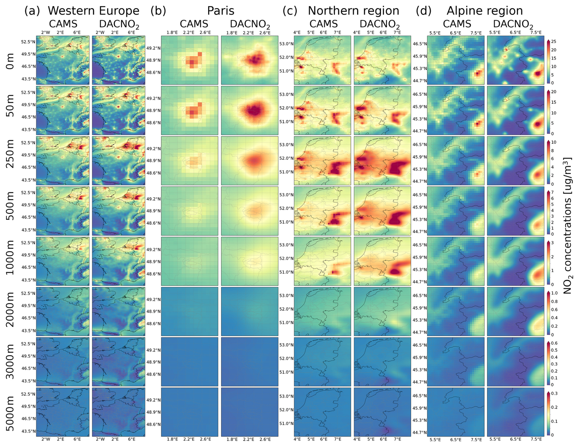
Figure 4 Annual mean NO₂ distributions for 2023 estimated from DACNO₂-Phase-3 (2 km × 2 km) and CAMS (10 km × 10 km) at multiple vertical layers. Layer-wise average NO₂ distributions over (a) Western Europe (entire study region), (b) Paris, (c) the northern region, and (d) the Alpine region.

Local-scale comparisons further highlight the advantages of DACNO₂ (Fig. 4b–d). In the Paris region (Fig. 4b), DACNO₂ provides finer spatial detail and greater NO₂ levels at lower altitudes (e.g., 0 m: 10.08 µg m⁻³; 50 m: 8.94 µg m⁻³; 250 m: 4.65 µg m⁻³), whereas CAMS results remain coarser with generally lower estimates (0 m: 8.43 µg m⁻³; 50 m: 7.15 µg m⁻³; 250 m: 3.63 µg m⁻³). In the northern region (Fig. 4c), DACNO₂ more distinctly resolves localized emission sources at low layers, capturing a greater number of hotspots than CAMS. As a result, the average NO₂ concentration from DACNO₂ is elevated throughout the boundary layer (up to 1000 m), with mean values 8.8 % higher than those from CAMS. In the Alpine region (Fig. 4d), DACNO₂ more effectively represents terrain-driven gradients and captures NO₂ enhancements within mountainous areas, demonstrating greater sensitivity to complex topographic influences. At higher altitudes, fine-scale variability diminishes in both models and their predicted NO₂ fields become more similar. This is because the influence of local emissions and surface features weakens, while regional-scale processes and long-range transport dominate (see Sect. 4.1). This reduced difference is also accompanied by much lower NO₂ concentrations at higher altitudes.

4 Insights and Implications of DACNO₂

4.1 Feature Importance and Data-driven Insights

We assessed the relative importance of input feature groups in DACNO₂ using the integrated gradients (IG) method (Sundararajan et al., 2017) implemented via the Captum interpretability library (Kokhlikyan et al., 2020). IG quantifies the effect of varying each input feature from a zero baseline to its actual value on a selected target function. In this analysis, we computed IG at two targets: (1) the RMSE between DACNO₂ predictions and 2023 EEA NO₂ training measurements at the surface, and (2) the RMSE between DACNO₂ predictions and 2023 CAMS NO₂ at multiple vertical layers. Feature group results are shown in Fig. 5, and results for individual features are provided in Fig. S9.

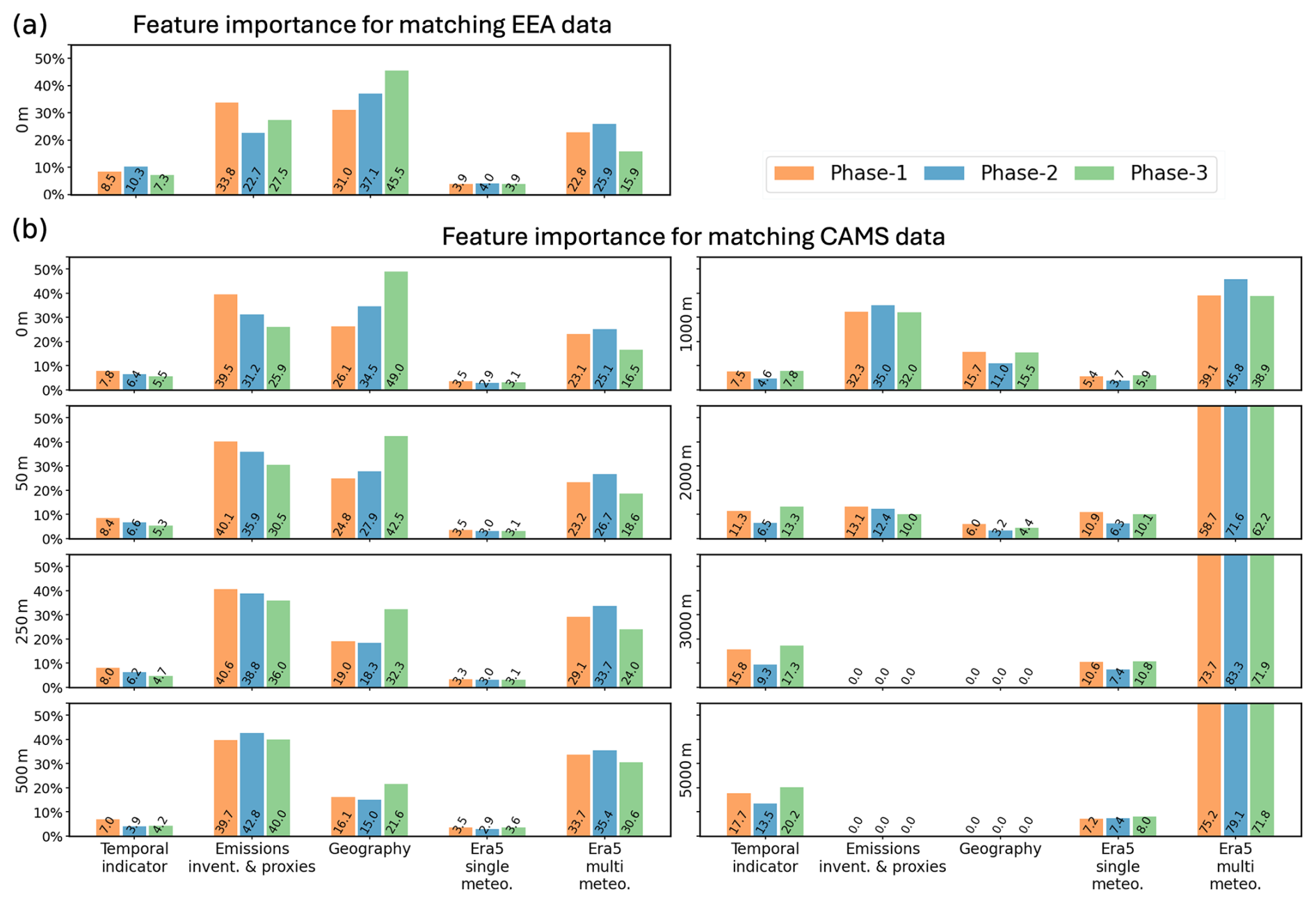
Figure 5 Relative importance of each input feature group for DACNO₂ model predictions, evaluated using the integrated gradients (IG) method. (a) Feature group contributions to RMSE between DACNO₂ surface NO₂ estimates and EEA ground-based measurements for 2023. (b) Feature group contributions to RMSE between DACNO₂ and CAMS NO₂ estimates at different vertical layers for 2023. The five feature groups are: temporal indicators, emission inventories and proxies, geography, ERA5 single-level meteorology, and ERA5 multi-level meteorology. Results are shown for each model training phase (Phase-1, Phase-2, and Phase-3), illustrating how the relative influence of input feature groups varies with training constraints and altitude. See Fig. S9 for the contributions of individual features within each group.

For surface NO₂ predictions evaluated against EEA measurements, DACNO₂ relies primarily on emission proxies, geographic features, and multi-level meteorological variables, while temporal indicators and single-level meteorological features play a lesser role. The addition of the EEA NO₂ constraint in Phase-2 and Phase-3 increases the importance of geographic data, highlighting its value for high-resolution surface NO₂ estimation. As shown in Fig. S9, land cover emerges as the most influential single feature (36.6 %) in DACNO₂-Phase-3. Multi-level meteorological variables dominate the meteorological contribution, suggesting partial redundancy between single-level and multi-level meteorological inputs.

For NO₂ estimates by layer evaluated against CAMS, the distribution of input feature importance at lower layers (up to 1000 m) is similar to that for surface NO₂ evaluated against EEA, suggesting that DACNO₂ remains relatively stable across training phases with different constraints. Differences between the three-phase models are most apparent near the surface but gradually diminish with height. The importance of geographic features steadily decreases with height, whereas emission features reach their strongest influence at approximately 500 m before declining. Above 3000 m, both become negligible, reflecting the transition from the Planetary Boundary Layer (PBL), which is influenced by local surface features, into the free troposphere, which is dominated by broad-scale processes. In contrast, temporal indicators, single-level meteorological features, and especially multi-level meteorological features become increasingly important with height. This shift highlights the greater reliance on temporal and large-scale atmospheric information for NO₂ estimates at higher layers. Among these features, radiation flux is the most important single-level meteorological variable, and wind is the dominant variable among all meteorological features (Fig. S9). Given the consistently low overall contribution of single-level meteorological variables, future model development may consider reducing or refining the use of this feature group to streamline the input space.

Overall, the DACNO₂ model is developed by combining multi-scale inputs and multi-source constraints. The fine-scale spatial structure on the 2 km grid is primarily informed by high-resolution emission-related proxies and geographic features, whereas large-scale spatiotemporal variation and vertical structure are driven by meteorological variables and temporal indicators. Through the phased training strategy, the CAMS constraint transfers large-scale spatiotemporal variation to the DACNO₂ model, and the EEA constraint guides the model to use fine-scale static inputs to shape this variation on the 2 km grid spatially.

4.2 Enhanced Vertical NO₂ Profile Representation

Figure 6 compares the average 2023 NO₂ profile estimates from DACNO₂-Phase-3 (2 km × 2 km) and CAMS (10 km × 10 km) for the Paris and Alpine regions, with results overlaid on Google Earth imagery for geographic context. In Paris, the regional average profile (Fig. 6a) indicates that DACNO₂ yields higher NO₂ concentrations up to 2000 m and steeper vertical gradients compared to CAMS. This enhancement likely results from DACNO₂'s use of high-resolution emission proxies and land cover information, allowing the model to resolve smaller and more localized emission sources (Kuik et al., 2018; Shahrokhishahraki et al., 2022). At the local scale, we take a transect over the grids of 100 km over Paris to compare the interpixel profile variability from CAMS and DACNO₂ (Fig. 6c). It is observed that DACNO₂ more clearly distinguishes spatial variability in the vertical structure, showing sharper contrasts and more pronounced local peaks than CAMS, particularly below 250 m. The regional average profiles for the Alpine area are similar between DACNO₂ and CAMS (Fig. 6b), which is due to the overall lower concentrations over this region with limited emission sources. However, local differences remain visible across a 200 km transect (Fig. 6d). DACNO₂ captures higher NO₂ concentrations around urban and small-scale hotspots, especially in valleys and canyons where pollutants tend to accumulate. Conversely, DACNO₂ provides lower NO₂ estimates in areas between the mountains with few sources. Overall, DACNO₂ provides more spatially detailed 3D NO₂ fields, revealing greater variability in the vertical profiles across different grids in this complex terrain. This refinement is important, as small point and line sources can contribute significantly NO₂ in mountainous regions (Kim et al., 2021).

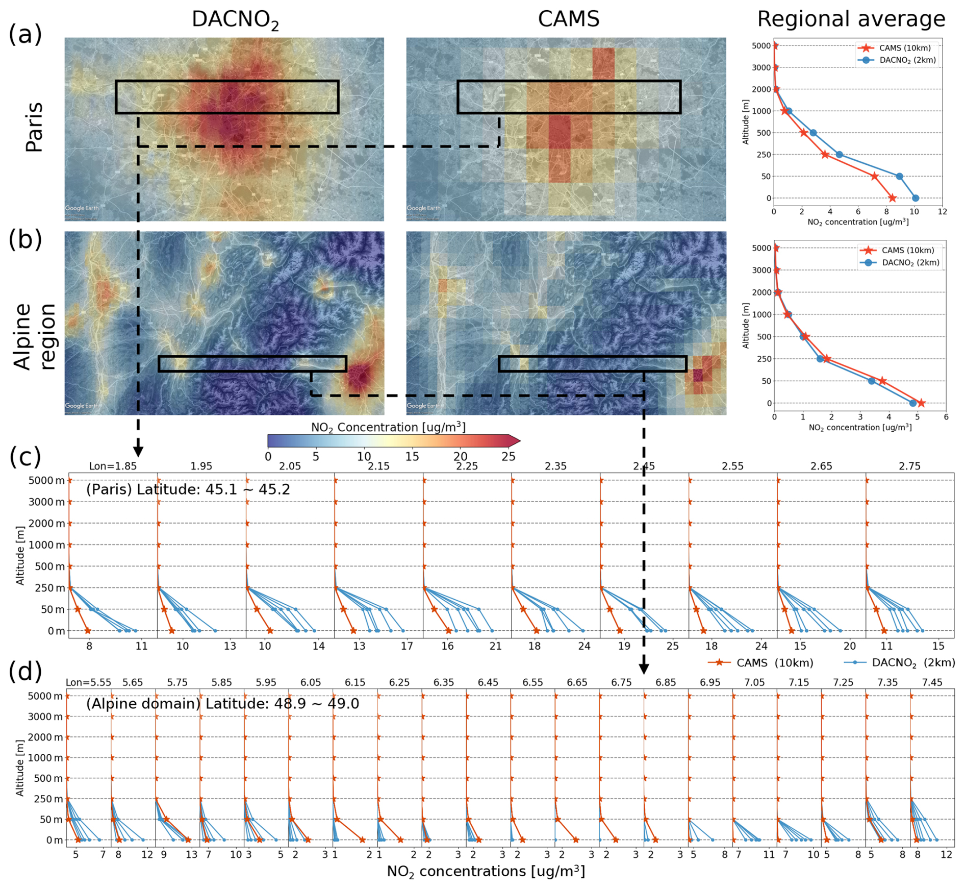
Figure 6 Comparison of NO₂ profile estimates from DACNO₂-Phase-3 (2 km × 2 km) and CAMS (10 km × 10 km) for the Paris and Alpine regions in 2023. Regional average vertical profiles and surface NO₂ distributions for Paris (a) and the Alpine region (b), with results shown over Google Earth imagery (Imagery © 2025 Airbus, Landsat/Copernicus, Map data © 2025 Google). Interpixel variability of NO₂ profiles from DACNO₂ and CAMS along a 100 km transect (black boxes) in the Paris area (c) and a 200 km transect in the Alpine region (d), illustrating local-scale differences in vertical structure.

To assess how vertical profiles differ between the two models across environments, we analyzed the mean DACNO₂-to-CAMS profile ratio across the entire study region in urban, suburban, rural, and uninhabited environments classified based on population density (Fig. S10) and the urbanization definition (Dijkstra et al., 2021). The results indicate that the DACNO₂-Phase-3 adjustment is not a uniform scaling of the CAMS field. Instead, near the surface, DACNO₂-Phase-3 shows higher concentrations relative to CAMS in urban regions (about 6 %) and lower concentrations in other areas (from about −20 % to −1 %). In the boundary layer (1000 m), the NO₂ concentrations are systematically higher in DACNO₂-Phase-3 compared to CAMS (from 10 % to 30 %), except in the uninhabited area (remains the same). At higher layers, DACNO₂-Phase-3 values converge to a lower ratio (about −22 % to −15 %) at 5000 m for the entire region. This behavior is also reflected in the layer-integrated column diagnostics shown in Fig. S11, which indicate near preservation of the regional column (0–5000 m), accompanied by a significant redistribution in the lower (0–1000 m) and conservative adjustment in upper (1000–5000 m) layers. Together, these results suggest that the DACNO₂-Phase-3 primarily redistributes NO₂ within the lower layers, enhancing horizontal contrast linked to human activity and emission strength, while maintaining consistently low estimates in the upper layers.

Additionally, we assessed the profile ratio across the three phases (Fig. S10). The results indicate that applying EEA constraints almost systematically increases NO₂ estimates in DACNO₂-Phase-2 relative to DACNO₂-Phase-1, likely because the CAMS data used for pretraining in Phase-1 underestimates NO₂ at EEA measurement stations. In contrast, the EEA constraint reduces NO₂ estimates in DACNO₂-Phase 3 relative to DACNO₂-Phase-2, consistent with the lower surface NO₂ levels observed in 2023 compared with the training years (2019, 2021, 2022, Fig. S7). However, the boundary-layer NO₂ estimates exhibit different trends that do not align with phase-dependent changes, which warrants further investigation.

In this work, the vertical structure of DACNO₂ is assessed through comparison with CAMS. Independent evaluation against vertically resolved observations, such as MAX-DOAS or aircraft measurements, would be the next step in future work. Such an analysis would require an hourly version of the DACNO₂ fields to provide daytime data and the application of appropriate observation operators to ensure comparability between the model and the observational data.

4.3 Implications for Satellite NO₂ Retrievals

To assess the potential of DACNO₂ for satellite NO₂ product improvement and development, we tested its use as a source of a-priori NO₂ profiles in TROPOMI retrievals. For this, a dedicated version of the model (DACNO₂-S5P) was developed for the TROPOMI overpass time, predicting a 3 h average NO₂ (11:00–13:00 UTC) using the same three-phase strategy. The model targets, named CAMS-S5P and EEA-S5P, represent process-based and measured NO₂ data during this period.

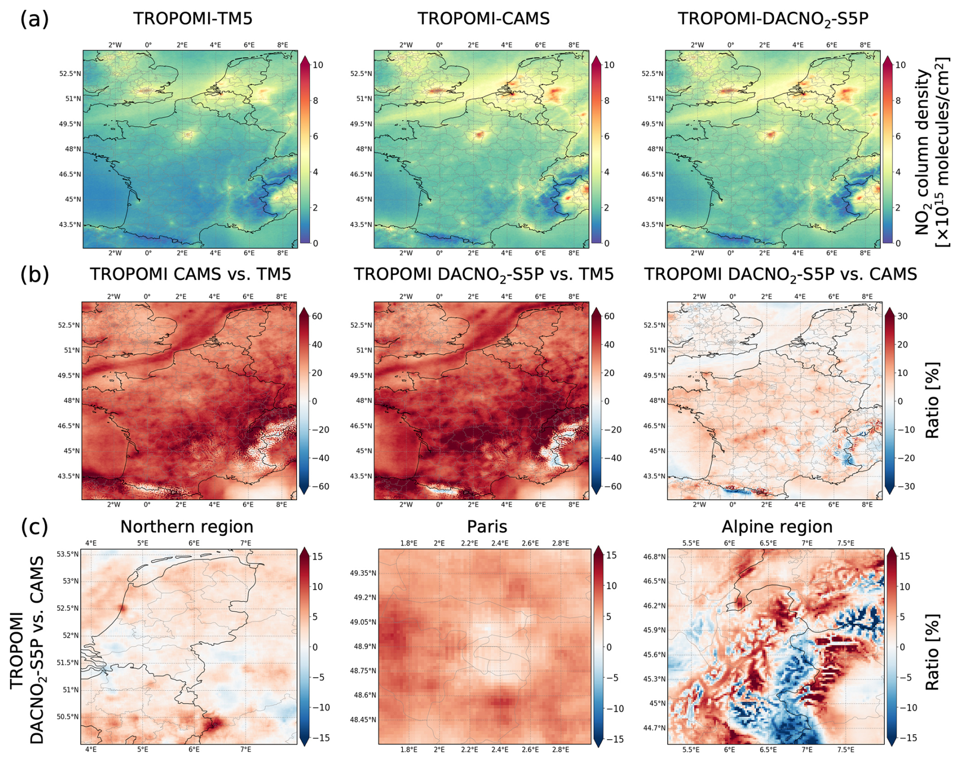
Figure 7 Impact of a-priori profile selection on TROPOMI tropospheric NO₂ column retrievals for 2023. (a) Annual mean TROPOMI NO₂ columns retrieved using the original TM5 (1° × 1°, approximately 100 km × 100 km), CAMS-S5P (10 km × 10 km), and DACNO₂-S5P (2 km × 2 km) a-priori profiles. (b) Spatial distribution of the relative difference (%) in TROPOMI NO₂ columns retrieved with three profiles. (c) The relative change in retrieved NO₂ columns across three subregions (the northern region, Paris, and the Alpine region) when using DACNO₂-S5P versus CAMS-S5P profiles.

Model evaluation (Table S1) shows DACNO₂-S5P agrees well with CAMS-S5P (RMSE = 0.98 µg m⁻³, r = 0.94, R²=0.88, bias = 0.03 µg m⁻³) on the 10 km grid. Compared to EEA-S5P measurements, DACNO₂-S5P achieves better agreement (RMSE = 5.07 µg m⁻³, r=0.77, R²=0.59, bias = 0.05 µg m⁻³) than CAMS-S5P (RMSE = 5.27 µg m⁻³, r = 0.76, R²=0.55, bias = −0.94 µg m⁻³).

We replaced the original TM5 a-priori profiles (1° × 1°, approximately 100 km × 100 km) in the TROPOMI retrievals with CAMS-S5P and DACNO₂-S5P profiles, following the approach described in Douros et al. (2023) and focusing on the troposphere. Figure 7a presents the annual mean TROPOMI NO₂ columns retrieved using these different a-priori profiles, with inter-comparisons shown in Fig. 7b and c. Both CAMS-S5P and DACNO₂-S5P profiles lead to substantial increases in the retrieved NO₂ columns, by 36.2 % and 39.8 % on average, respectively. The increase associated with CAMS-S5P is consistent with previous findings (Douros et al., 2023) and is primarily attributable to the improved spatial resolution of the a-priori profile, which better represents near-surface NO₂ enhancements and fine-scale spatial gradients, resulting in larger retrieved tropospheric columns over emission hotspots (Tack et al., 2021; Ialongo et al., 2020).

Compared to the CAMS-S5P profile, using DACNO₂-S5P as the a-priori increases retrieved NO₂ columns by about 3.0 % on average (Fig. 7b), associated with the reduced negative bias against EEA-S5P measurements reported above. This change is accompanied by a clear spatial structure in the differences, with localized increases over small-scale emission hotspots and decreases over low-emission regions. In central-western France (0–2.6° E, 45.6–46.3° N), a distinct southwest-to-northeast line of reinforced NO₂ columns appears because DACNO₂-S5P enhances the emission signals from the cities of Angoulême, Guéret, and Montluçon. Regional comparisons (Fig. 7c) show that the DACNO₂-S5P profile leads to a 1.8 % increase in the northern region and 5.9 % in Paris, with the most significant increases surrounding major emission hotspots. This is likely due to DACNO₂'s enhanced ability, based on finer resolution, to capture small-scale emission sources and resolve strong spatial gradients around NO₂ hotspots. In the Alpine region, the average increase reaches 1.7 %, ranging from −18.1 % (5th percentile) to +24.1 % (95th percentile) between the surrounding areas and the central mountains, with a similar pattern observed in the Pyrenees. The absolute difference remains small, ranging from −3.94 × 10¹⁴ molecules cm⁻² (5th percentile) to 5.39 × 10¹⁴ molecules cm⁻² (95th percentile). This large fluctuation reflects the complex NO₂ distribution in the mountainous region and benefits from high-resolution modeling, as DACNO₂ estimates can reach lower background values or enhance the hotspots signal in this region.

These results illustrate the potential of using DACNO₂ profiles to improve satellite NO₂ retrievals, particularly for evolving high-resolution instruments. However, the DACNO₂ product remains a prototype, and we outline a brief roadmap for operational deployment in the conclusion section. In addition, DACNO₂ provides a-priori NO₂ profiles up to 5000 m, while NO₂ levels at roughly 8–12 km show a slight enhancement, possibly linked to aviation and lightning (Douros et al., 2023; Kuhn et al., 2024a; Dahlmann et al., 2011; Richter, 2009). This should also be considered in future DACNO₂ development.

4.4 Generalization Capability and Data Quality: Insights from the COVID-19 Period

As noted in Sect. 2.4.1, CAMS NO₂ data for 2020 were excluded from the training set based on preliminary experiments showing that their inclusion substantially reduced model generalization at higher layers. Since 2020 was marked by the COVID-19 pandemic and large reductions in anthropogenic emissions (Levelt et al., 2022), we specifically evaluated DACNO₂'s predictive performance for this anomalous year. To this end, the DACNO₂-Phase-2 model was fine-tuned on 2020 EEA NO₂ data, following the same phased development strategy, to produce DACNO₂-Phase-3-2020.

Table 3 summarizes the 2020 evaluation results, following the format of Table 2. Both DACNO₂-Phase-2 and DACNO₂-Phase-3-2020 reproduced observed surface NO₂ concentrations well (e.g., DACNO₂-Phase-3-2020: RMSE = 5.47 µg m⁻³, r = 0.82, R² = 0.67, bias = 0.01 µg m⁻³), with performance comparable to CAMS (RMSE = 4.99 µg m⁻³, r = 0.88, R²=0.73, bias = −2.05 µg m⁻³) but notably lower bias. Figure S5 shows the temporal trend between model estimations and EEA measurements. It is observed that DACNO₂-Phase-2 can still capture the temporal trend of NO₂ in this unknown and anomalous year, while a positive bias appears during March and May when COVID-19 control measures took place. DACNO₂-Phase-3-2020 has successfully reduced the remaining bias with the adaptive fine-tuning. This demonstrates the robustness of the DACNO₂ model and the necessity of adaptive fine-tuning to capture anomalous events. Additionally, CAMS maintains overall consistency across measurements but exhibits a pronounced negative bias, primarily in urban areas.

Table 3 Performance of DACNO₂ on the 2020 dataset.

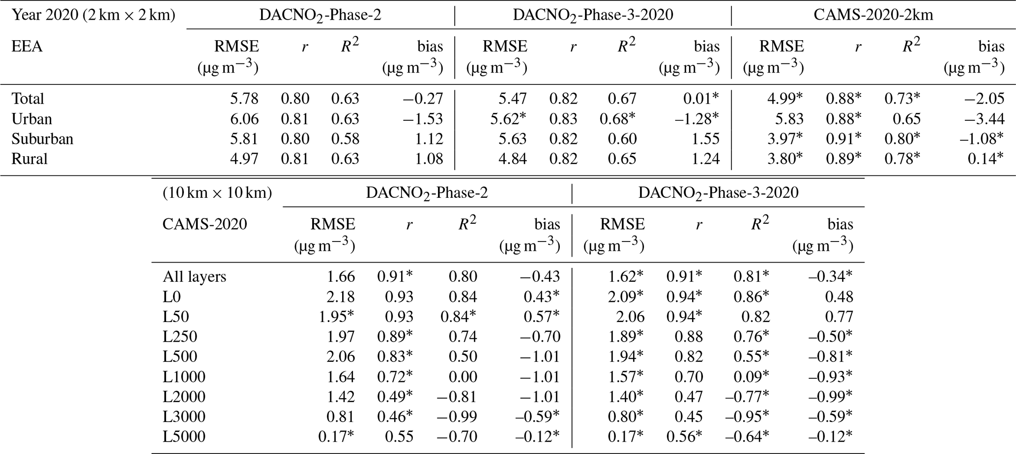
Note: Similar to Table 2, but for the year 2020.

Agreement between DACNO₂ and CAMS remains strong at low altitudes (e.g., surface: RMSE = 2.09 µg m⁻³, r = 0.94, R²= 0.86, bias = 0.48 µg m⁻³), but declines rapidly above 1000 m, where R² values approach zero or become negative, indicating a failure to reproduce high altitude CAMS NO₂ distributions for 2020. Comparison of CAMS NO₂ vertical distributions from 2019 to 2023 (Fig. S2) shows generally consistent annual patterns, except for 2020, which is characterized by anomalously high values above 1000 m. This anomaly is also noted in the CAMS 2020 annual evaluation report (Meleux et al., 2023), which attributes it to some sub-models producing unexpectedly high NO₂ in the upper layers, resulting in inflated tropospheric column estimates. The underlying causes remain unresolved and require further investigation. These findings highlight the importance of data screening, such as checking distributions and identifying outliers, before model training. Including biased or anomalous target data can introduce noise, increase the risk of overfitting, and reduce generalization performance.

5 Conclusions and Outlook

This study presents the Deep Atmospheric Chemistry NO₂ model (DACNO₂), a deep learning model for daily, high-resolution (2 km × 2 km) 3D NO₂ estimation. DACNO₂ integrates multi-source and multi-modal input features, including emissions, geography, meteorology, and temporal indicators. It uses a multi-constraint and phased training approach to learn from both process-based CAMS NO₂ and measured EEA NO₂ data. This approach allows DACNO₂ to reproduce broad-scale, process-based NO₂ patterns and capture local NO₂ gradients. Results show that DACNO₂ significantly improves the ability to resolve fine-scale spatial patterns, near-surface NO₂ variability, and vertical distribution. It also generalizes well across different spatial areas (urban, rural, mountainous, and emission hotspot regions) and periods of anomalous emissions. At the 2 km grid resolution, most spatial detail is provided by high-resolution, time-independent geographic data and emission-related proxies. Meanwhile, large-scale variability is driven primarily by meteorological variables and temporal indicators at coarse scales. The DACNO₂ model learns, through a phased training strategy, how these dynamic coarse-scale drivers interact with fine-scale spatial inputs to improve the spatiotemporal representation of the NO₂ variability. Furthermore, the framework demonstrates transferability and flexibility, allowing the model to be fine-tuned to adapt to future emission scenarios and to be adjusted to produce outputs for specific satellite overpass times in addition to daily averages.

A systematic evaluation shows that DACNO₂ outperforms the state-of-the-art regional CAMS product in reproducing measured surface NO₂ concentrations. Overall, DACNO₂ achieves a lower RMSE (4.99 vs. 5.32 µg m⁻³), higher correlation (r = 0.82 vs. 0.80, R²=0.66 vs. 0.61), and a substantially reduced bias (−0.38 vs. −1.15 µg m⁻³). The improvement is most evident at urban sites, where spatial variability is strongest, and DACNO₂ also reduces the positive bias at rural sites with low background concentrations. Vertical profile analysis indicates that DACNO₂ provides greater spatial detail and variation than CAMS, capturing small-scale emission sources and topographic influences more effectively. Feature importance analysis indicates that high-resolution emission proxies, land cover, and multi-level meteorological variables are key contributors to constructing spatial and vertical NO₂ patterns. In contrast, single-level meteorological variables provide only limited incremental information, likely due to some redundancy with the multi-level data, suggesting opportunities for future model optimization. In addition, the EEA-based examination indicates that future EEA constraint usage should consider sample rebalancing and provide sufficient spatial context.

Application to satellite NO₂ retrievals demonstrates that using DACNO₂-generated a-priori profiles makes the TROPOMI NO₂ products better account for near-surface concentrations and emission hotspots, particularly for small-scale emission sources and complex geographic regions. These findings underscore the potential of high-resolution ML-based profiles for future high-resolution satellite retrievals. However, DACNO₂ remains a prototype, and further work is needed for operational deployment. First, this would involve extending the model's output to continuous hourly profiles across a broader geographic domain and considering profiles above 5000 m. Second, the model would need to be operated on a robust GPU computational platform with automated data pipelines. Third, a routine validation framework would need to be established to continuously monitor performance against various data, such as CAMS NO₂, EEA NO₂, and vertical measurements (e.g., MAX-DOAS). Finally, this operational system would require a strategy for periodic model fine-tuning to adapt to evolving emission patterns and maintain long-term accuracy.

Analysis of model performance during COVID-19 indicates that DACNO₂ consistently generalizes well despite emission anomalies. The inconsistencies observed in CAMS reanalysis for 2020 at high layers highlight the need for screening and quality assurance in model training data to avoid learning biased patterns and degrading model reliability.

The constraint strategy still needs improvement, as the model's fine-tuning currently relies heavily on surface EEA measurements, which are biased due to uneven distribution, measurement methods, and spatial representativeness. Future development of DACNO₂ could incorporate constraints above the surface, such as integrating high-resolution 3D process-based NO₂ fields from models (e.g., WRF-Chem) and column observations from satellites, and embedding additional physical constraints into the loss function. Moreover, one can explore transformer architectures for improved scalability and multimodal data processing, and extend the model to continental or global applications (including data-poor regions such as the African continent). This will further support large-scale air quality management and atmospheric chemistry research.