The impact of the stratospheric quasi-biennial oscillation on Arctic polar stratospheric cloud occurrence

Polar stratospheric clouds (PSCs) play a critical role in stratospheric ozone depletion. Previous studies have shown that the quasi-biennial oscillation (QBO) influences the Arctic stratospheric polar vortex and ozone, yet few studies have thoroughly analyzed the impact of the QBO on Arctic PSC occurrence. This study examines this impact using CALIPSO observations from 2006 to 2021 and SLIMCAT simulations from 1979 to 2022. The results show that the winter PSC coverage area is significantly larger during the westerly QBO (WQBO) phase than during the easterly QBO (EQBO) phase, with a zonal asymmetry in PSC occurrence frequency anomalies. The QBO influences the temperature, water vapour (H₂O), and nitric acid (HNO₃) in the Arctic stratosphere, which are key factors affecting PSC formation. During the WQBO phase, Arctic stratospheric temperatures show negative anomalies, with the centre of this anomaly biased towards North America. In addition, H₂O shows positive anomalies in the Arctic lower stratosphere, mainly due to the stronger polar vortex preventing the transport of high-moisture air at high latitudes to mid-latitudes, causing H₂O to accumulate inside the polar vortex. HNO₃ shows negative anomalies, primarily caused by denitrification through nitric acid trihydrate (NAT) sedimentation. Sensitivity analyses further indicate that QBO-induced temperature anomalies are the dominant driver of PSC variability, while the direct effect of H₂O anomalies on PSCs is relatively small. The reduction of HNO₃ mainly affects PSCs in February and March. This work implies that future changes in the QBO may influence ozone by affecting PSCs.

1 Introduction

Polar stratospheric clouds (PSCs) form at low temperatures in the lower and middle polar stratosphere during winter and early spring, and their particle surfaces provide sites for heterogeneous chemical reactions that can convert chlorine reservoir species (HCl, ClONO₂, etc.) into active forms (Cl, ClO, etc.). When spring arrives, these reactive chlorine atoms participate in the Cl_x (= Cl + ClO + 2Cl₂O₂) catalytic cycles that destroy stratospheric ozone (Solomon et al., 1986, 2015). Previous studies have shown that there exists a linear relationship between ozone loss and the volume of PSCs exposed to sunlight (Rex et al., 2004; Pommereau et al., 2018). Therefore, the PSCs play an important role in the Antarctic ozone hole and Arctic stratospheric ozone depletion. Over the past four decades, since the emergence of ozone depletion, much research has been conducted on PSCs (e.g., McCormick et al., 1982; Schreiner et al., 2002; Lowe and MacKenzie, 2008; Pitts et al., 2018; Voigt et al., 2018; Tritscher et al., 2021). According to their composition and physical phase state, PSCs are classified into three basic types (Browell et al., 1990; Toon et al., 1990; Carslaw et al., 1994; Hanson and Mauersberger, 1988; Tritscher et al., 2021): nitric acid trihydrate (NAT), supercooled ternary solution (STS; Tabazadeh et al., 1994), and ice. The formation processes of these three PSC types differ significantly and are strongly temperature-dependent. STS forms from stratospheric sulfuric acid aerosols (SSA) in the global Junge layer, which is located around 20 km and composed of sulfuric acid (H₂SO₄) and water (Junge et al., 1961). As the temperature decreases in polar winter, the SSA grows by absorbing nitric acid (HNO₃) and water vapour (H₂O) until the temperature drops to about 192 K to form STS. The formation of ice can occur via two pathways: one is homogeneous nucleation at a supercooling of ∼ 3 K below the ice frost point T_ice (∼ 184 K) (Carslaw et al., 1998; Koop et al., 1998), while the other is heterogeneous nucleation below T_ice (Engel et al., 2013; Voigt et al., 2018). NAT can form on the pre-existing ice particles (Carslaw et al., 1998; Wirth et al., 1999) or on the SSA particles containing meteoritic dust (Lambert et al., 2016) or wildfire smoke (Ansmann et al., 2022). The existence temperature of NAT (T_NAT) is not too low, typically around 195 K. However, studies show that heterogeneous chlorine activation occurs predominantly on STS (Wegner et al., 2012), which does not mean that the NAT and ice are not important for ozone depletion. In contrast, NAT and ice can redistribute the HNO₃ and H₂O in the polar stratosphere through sedimentation, which will affect further PSC formation as well as ozone depletion (Hunt, 1966; Nicolet, 1970; Salawitch et al., 1993).

The formation of PSCs is primarily influenced by temperature and concentrations of H₂O, HNO₃, and H₂SO₄ in the gas phase (Leroux and Noel, 2024). It is noteworthy that the temperature and chemical species in the polar stratosphere are not only influenced by polar physical and dynamical processes but also by the tropical atmosphere (Strahan et al., 2009; Bittner et al., 2016; Matsumura et al., 2021). The quasi-biennial oscillation (QBO) is the dominant mode of variability in the tropical stratosphere (Hansen et al., 2013) and one of the major external drivers of the wintertime polar vortex in the Northern Hemisphere (NH) stratosphere (Garfinkel et al., 2012). The QBO is characterized by an alternating pattern of easterly and westerly winds propagating downward through the tropical stratosphere, with a period of approximately 28 months. It is primarily driven by upward-propagating gravity waves, inertia-gravity waves, Kelvin waves, and Rossby-gravity waves (Holton and Lindzen, 1972; Plumb, 1977; Dunkerton, 1997; Baldwin et al., 2001).

Many studies based on observations or reanalysis (Holton and Tan, 1980; Lu et al., 2014; Yamazaki et al., 2020) and numerical models (Garfinkel et al., 2012; Hansen et al., 2013; Elsbury et al., 2021) indicate that the NH polar vortex is weaker during the easterly QBO (EQBO) phase compared to the westerly QBO (WQBO) phase, which is known as the “Holton-Tan (HT) effect” (Holton and Tan, 1980). Various explanations have been proposed to account for this phenomenon, which can be categorized into two mechanisms. The first mechanism, proposed by Holton and Tan (1980, 1982), suggests that the QBO affects the NH polar vortex by adjusting the position of the critical line (i.e., zero wind line). During the EQBO phase, the critical line is shifted to the NH subtropics, which reflects more planetary waves toward the Arctic, weakening the polar vortex. In contrast, during the WQBO phase, the critical line located in the Southern Hemisphere (SH) allows more planetary waves to propagate toward the equator, resulting in a stronger Arctic stratospheric polar vortex (Lu et al., 2014). However, another mechanism suggests that the critical line mechanism is not important in the HT effect, arguing that meridional circulation induced by QBO can affect the propagation of planetary waves by influencing the wave refraction index (Garfinkel et al., 2012; White et al., 2016). Overall, the QBO influences the strength and temperature of the NH polar vortex through the dynamical interactions between wave and mean flows. Furthermore, studies have shown that the frequency of sudden stratospheric warmings (SSWs) in the Arctic is higher during the EQBO phase than during the WQBO phase (Holton and Tan, 1980; Salminen et al., 2020), which has a significant impact on the polar vortex and temperature. Since PSCs are temperature-sensitive, the QBO may have a potential influence on PSC occurrence by influencing the polar vortex.

On the other hand, the QBO also influences stratospheric chemical species through dynamical and chemical processes. Previous studies have focused on the impact of the QBO on stratospheric chemical species such as ozone, H₂O, and methane (CH₄) (Hansen et al., 2013; Tweedy et al., 2017; Zhang et al., 2021; Wang et al., 2022). Among these, the transport of dynamical processes is the primary pathway by which the QBO affects stratospheric chemical species. For instance, some studies have linked anomalies in tropical stratospheric chemical species to vertical motion anomalies induced by the QBO. During the EQBO phase, anomalous upward motion in the lower tropical stratosphere induced by the QBO leads to the transport of ozone-poor air from the troposphere into the lower stratosphere, resulting in a negative ozone anomaly in the lower tropical stratosphere (Gray and Pyle, 1989; Butchart et al., 2003; Zhang et al., 2021). In contrast, during the WQBO phase, the weakening of the upward motion results in a positive ozone anomaly in the lower tropical stratosphere. Furthermore, the QBO's influence on the tropical secondary circulation also affects the transport of other gases into the stratosphere, such as CH₄ (Xia et al., 2019), HCl (Chen et al., 2005), and N₂O (Park et al., 2017). Notably, H₂O entering the stratosphere is influenced by the temperature of the tropical tropopause (cold point temperature), which can lead to the condensation and dehydration of H₂O (Holton and Gettelman, 2001; Tian et al., 2019; Keeble et al., 2021). Anomalous upward motion near the tropopause during the EQBO phase leads to a decrease in the cold point temperature, thereby reducing the amount of H₂O entering the stratosphere. Consequently, a negative H₂O anomaly is observed in the lower tropical stratosphere during the EQBO phase (Hansen et al., 2013; Diallo et al., 2022). In addition to modulating the ascent of the Brewer-Dobson (BD) circulation in the tropics and affecting the distribution of chemical species in the tropical stratosphere, the QBO may also influence the downward branch of the BD circulation to further affect the chemical composition in high-latitude regions of the stratosphere. Hansen et al. (2013) found that, compared to the EQBO phase, the downward branch of the BD circulation in the polar regions above the tropopause is weakened during the WQBO phase, leading to less H₂O being transported downward to the tropopause, which results in the accumulation and a positive anomaly of H₂O in the Arctic lower and middle stratosphere.

Compared to dynamical processes, the QBO has a relatively small impact on stratospheric species through chemical processes, primarily affecting reaction rates by modulating temperature. Previous studies have shown that temperature anomalies in the lower tropical stratosphere induced by the QBO contribute to ozone anomalies to some extent (Ling and London, 1986; Zhang et al., 2021). Additionally, Zhang et al. (2021) found that during the EQBO phase, a reduction in PSCs associated with QBO-induced warming weakens heterogeneous chemical processing, leading to a decrease in active chlorine and an increase in ozone in the Arctic lower stratosphere. It is worth noting that their study primarily focused on the dynamical and chemical effects of the QBO on stratospheric ozone, without a detailed exploration of the QBO's impact on PSCs. Given that the QBO not only influences the temperature in the Arctic lower stratosphere but also affects chemical species, these key factors can impact the formation of PSCs. However, no study has deeply investigated the processes and mechanisms of the QBO effects on PSCs. From 2006 to 2021, the Cloud-Aerosol Lidar and Infrared Pathfinder Satellite Observations (CALIPSO) mission continuously observed PSCs over both the Arctic and Antarctic, providing an unprecedented view of PSC occurrence and composition (Tritscher et al., 2021). In this study, we utilize CALIPSO PSC observations (Pitts et al., 2018) to investigate the potential impact of the QBO on Arctic PSC occurrence. However, the CALIPSO record includes only 15 Arctic winters, which may limit the statistical robustness of the results – for instance, the results could be affected by extreme events. To address this limitation, we also incorporate simulations from the SLIMCAT 3D chemical transport model, which spans over 40 years from 1979 to 2022, to complement the observational analysis.

2 Data and methods

2.1 Data

2.1.1 PSC observations

As a part of the A-Train, CALIPSO provides global profiling of aerosols and clouds in the troposphere and lower stratosphere. Following its launch in 2006 and operating continuously until 2023, CALIPSO collected data nearly every day along 14–15 orbits between 82° S and 82° N (Winker et al., 2009). The Cloud-Aerosol Lidar with Orthogonal Polarization (CALIOP) aboard CALIPSO is a dual-wavelength polarization-sensitive lidar that simultaneously produces linearly polarized pulses at 532 and 1064 nm and receives both parallel and perpendicular components of the 532 nm return signal (orthogonal polarization channels), as well as the total 1064 nm return signal (Winker et al., 2007). The depolarization measurements of CALIOP make it possible to distinguish between spherical and non-spherical aerosols (Sassen, 1991), and the signal strength also being influenced by aerosol particle size. Due to the differences in morphology (aspect ratio) and size of the various components of PSC particles, CALIOP can classify PSC particles. Based on this principle, Pitts et al. (2007) developed a PSC classification algorithm using CALIOP data, which has been continuously refined and optimized in subsequent years (Pitts et al., 2009, 2011, 2013, 2018).

In this study, we use the latest CALIPSO Level 2 Polar Stratospheric Cloud Mask V2.00 product (Pitts et al., 2018) from 2006 to 2021, which includes five types of PSCs (STS, NAT-mix, Ice, NAT-enhanced, and wave ice) along CALIPSO orbit tracks and has been widely used to study the characteristics of PSCs and to compare them with model simulations to improve the representation of PSCs in global models (e.g. Tritscher et al., 2021; Zhao et al., 2023; Li et al., 2024). The data span altitudes from 8.4 to 30 km, with a vertical resolution of 180 m and a horizontal resolution of 5 km. Benefiting from CALIPSO's polar orbit, the number of observations in the polar regions is significantly higher than in the mid- and low-latitude regions.

2.1.2 Aura MLS measurements

The Microwave Limb Sounder (MLS), on board the National Aeronautics and Space Administration (NASA) Aura satellite launched on 15 July 2004, uses microwave limb sounding technology to provide information from the upper troposphere to the mesosphere (Waters et al., 2006). Aura MLS takes measurements approximately every 25 s, recording atmospheric parameters such as temperature and atmospheric constituents from the surface to 90 km. It generates about 3500 scans per day, covering latitudes from 82° S to 82° N (Livesey et al., 2006; Read et al., 2006, Livesey et al., 2021). In this study, we use MLS V5.0, Level 3 H₂O and HNO₃ from 2004 to 2022. H₂O is retrieved using 190 GHz radiation, with the recommended vertical range of 316 to 0.00215 hPa and accuracy between 6 % and 22 % in the stratosphere. HNO₃ is retrieved using 190 GHz (below 22 hPa) and 240 GHz (above or equal to 22 hPa) radiation, with a recommended vertical range of 215 to 1.5 hPa and an uncertainty range of approximately 0.1 to 2.2 ppbv. V5 data, as recommended by the MLS science team, show improved accuracy over V4, particularly in reducing H₂O drift by about 2–4 % per decade (Livesey et al., 2021). Additionally, we utilize daily level 3 data from MLS V5, which are gridded datasets generated by applying a simple “binning” method to the level 2 orbital data.

2.1.3 Reanalysis data

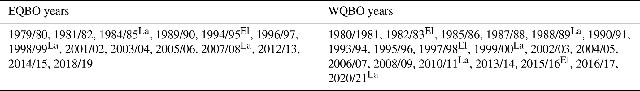
The European Centre for Medium-Range Weather Forecasts (ECMWF) ERA5 reanalysis data for temperature and wind from 1979 to 2022 are used in this study, with a spatial resolution of 1° latitude × 1° longitude and 37 levels from 1000 to 1 hPa (Hersbach et al., 2020). The QBO index and the BD circulation are calculated using this dataset. Consistent with previous studies (Zhang et al., 2021), the QBO index in this study is defined as the standardized zonal mean wind between 10° S and 10° N at 50 hPa. The WQBO phase is defined as the QBO index in December greater than 0.5, and the EQBO phase is defined as less than −0.5. The dataset from 1979 to 2022 includes 14 EQBO phases from December to March and 19 WQBO phases (see Table 1). “El” and “La” in Table 1 refer to the years with strong El Niño and La Niña events, respectively, defined by an Oceanic Niño Index (ONI, https://cpc.ncep.noaa.gov/products/analysis_monitoring/ensostuff/ONI_v5.php, last access: 18 November 2025) (Glantz and Ramirez, 2020) greater than 1 °C or less than −1 °C during winter.

Table 1 List of EQBO and WQBO years from December to March during the study period (1979–2022).

2.2 SLIMCAT Model

TOMCAT/SLIMCAT (hereafter SLIMCAT) is an offline three-dimensional chemical transport model (CTM). It is forced by the ECMWF ERA5 winds and temperatures, which are interpolated to the model grid with a horizontal resolution of 2.8° × 2.8° and a total of 32 levels from the surface to ∼ 60 km (Feng et al., 2021). The model contains a detailed description of stratospheric chemistry, including heterogeneous reactions on sulfate aerosol and PSC surfaces. It has been widely used in studies of the dynamical transport and chemical reactions in the stratosphere (Dhomse et al., 2011; Chipperfield et al., 2017; Weber et al., 2021) and has been shown to accurately simulate key stratospheric chemical species (Feng et al., 2021; Li et al., 2022). The standard version of the model uses a simplified thermodynamic equilibrium PSC scheme, which includes the parameterization of liquid sulfate aerosols (LA, including binary sulfate aerosols and supercooled ternary solution, STS), solid nitric acid trihydrate (NAT), and ice. The model calculates the equilibrium vapor pressure of H₂SO₄ using the expression from Ayers et al. (1980), and when the H₂SO₄ concentration exceeds the equilibrium vapour pressure, sulfate aerosol is considered to be present. Notably, the stratospheric H₂SO₄ in the model is not provided by initial conditions but is instead calculated based on an assumed number density (10 cm⁻³) of sulfate aerosol, with the stratospheric aerosol surface area density (SAD) derived from ftp://iacftp.ethz.ch/pub_read/luo/CMIP6 (last access: 18 November 2025; Arfeuille et al., 2013; Dhomse et al., 2015; Feng et al., 2021). This scheme also calculates the concentrations, mass fractions, and solubilities of H₂SO₄, HNO₃, HCl, HBr, HOCl, and HOBr in liquid aerosols (Carslaw et al., 1995a, b).

The presence of NAT and ice is determined based on HNO₃, H₂O, and temperature using expressions from Hanson and Mauersberger (1988). NAT is considered to be present when the concentration of HNO₃ exceeds 10 times its equilibrium vapour pressure (Grooß et al., 2018). The model assumes that NAT particles exist in two modal radii (0.5 and 6.5 µm), and the SAD required for heterogeneous reactions is derived from small-radius NAT particles calculated by the condensable amount of HNO₃, with a limit of 1 cm⁻³ for the number density of small particles. The remaining HNO₃ condenses into large-radius NAT particles (Davies et al., 2002; Feng et al., 2005). Ice is assumed to form when H₂O concentration exceeds its equilibrium vapour pressure, and the model assumes a number density of 10 cm⁻³ for ice particles, with their SAD calculated from the condensable amount of H₂O. The model also uses simplified denitrification and dehydration schemes, with large-radius NAT particles and ice particles assumed to settle at velocities of 1100 and 1500 m d⁻¹, respectively (Feng et al., 2011), to redistribute HNO₃ and H₂O.

In this study, we use SLIMCAT to simulate the period 1979–2022. In addition, fixed ozone-depleting substances (ODS) for the year 2000 and climatologies of sulfate aerosol SAD and solar flux were used to exclude the effects of variations in sulfate aerosol SAD, solar flux, and anthropogenic ODS emissions. Based on the Arctic winter and early spring HNO₃ and H₂O derived from SLIMCAT, we diagnosed offline the equilibrium temperature of NAT (T_NAT) according to Hanson and Mauersberger (1988), which is the warmest temperature at which PSC particles can theoretically start to form and persist (Tritscher et al., 2021; Leroux and Noel, 2024). We consider PSCs to be present when the temperature at the grid point falls below T_NAT and calculate the PSC coverage areas. These areas, based on T_NAT, are the theoretical maximum areas of PSC. Li et al. (2024) showed that the PSC area derived from SLIMCAT is in good agreement with CALIPSO observations in terms of seasonal evolution, interannual variability, and spatial distribution. This strengthens confidence in the performance of the SLIMCAT model in simulating PSCs.

2.3 PSC area and volume calculation

In this study, two different methods are used to calculate the daily PSC coverage areas of CALIPSO and SLIMCAT, respectively. For SLIMCAT, the PSC coverage area is computed by summing the areas of model grid cells containing PSCs, hereafter referred to as the “Grid method”. Since CALIPSO observations of PSCs along its orbit do not cover all model grid cells, the CALIPSO PSC area is calculated using a statistical method referred to Pitts et al. (2018) (hereafter, the “P18 method”), which divides 50–90° N into 10 latitude bands, and the PSC area is estimated as the sum of the occurrence frequency of PSC in the 10 latitude bands multiplied by the area of each band. Li et al. (2024) compared the differences in SLIMCAT PSC areas calculated using the “Grid method” and the “P18 method”. They indicated that the areas derived from both methods are similar. However, when the “P18 method” is used, the daily variability in the SLIMCAT PSC area increases slightly. To avoid this issue, the “P18 method” is used to calculate the PSC coverage areas of CALIPSO, while the “Grid method” is applied to SLIMCAT.

The PSC volume is then derived by vertically integrating the PSC area from CALIPSO, MIPAS, and SLIMCAT. For MIPAS, the PSC area is calculated using the “P18 method” applied to all PSC detections up to 6 km below the cloud top height (Spang et al., 2018).

3 Results

3.1 Impact of QBO on Arctic PSCs

Figure 1a shows the interannual variation of Arctic PSC volume anomalies from CALIPSO and MIPAS observations and SLIMCAT simulations. Due to CALIPSO's higher detection threshold, the observed PSC volume is significantly smaller than the volumes of MIPAS and SLIMCAT (Li et al., 2024). Nevertheless, all three datasets exhibit remarkably consistent interannual variability in PSC volumes, indicating that the SLIMCAT model realistically captures observed interannual variation in Arctic PSC. Figure 1b and c (left) show the relationship between the Arctic PSC volume and the QBO index of December. Due to the limited number of MIPAS samples, we only perform linear regression on the PSC volume and QBO index for CALIPSO and SLIMCAT. Both CALIPSO and MIPAS observations and SLIMCAT simulations show that the PSC volume increases with increasing QBO index. However, the CALIPSO PSC volume does not show a statistically significant correlation with the QBO index (p = 0.38), with the limited sample size of satellite observations likely contributing to this result. In contrast, the SLIMCAT PSC volume shows greater variation with the QBO index, and the regression line passes the significance test (p = 0.01), likely due to the larger sample size. In addition to the correlation, the probability distribution of the PSC volume also shows a distinct difference between the WQBO and EQBO phases. During the EQBO phase, a large portion of the PSC volume is near zero. For example, of the 14 SLIMCAT simulations, 5 show values below 1×10⁶ km³. In contrast, during the WQBO phase, all SLIMCAT simulations exceed 1×10⁶ km³. The probability distribution functions (PDF) of the PSC volume during the WQBO and EQBO phases also support the above conclusions (right panel of Fig. 1b and c). The results show that the PDFs of PSC volume during both WQBO and EQBO phases exhibit skewed distributions. Compared to the WQBO, the PSC volume during the EQBO phase shifts to smaller values, suggesting that the tropical QBO can influence Arctic PSC. Note that large PSC volumes can occur during the EQBO phase, because the Arctic stratospheric vortex is influenced not only by the QBO but also by other factors, such as ENSO (Brönnimann et al., 2004; Garfinkel and Hartmann, 2008; Zhang et al., 2022).

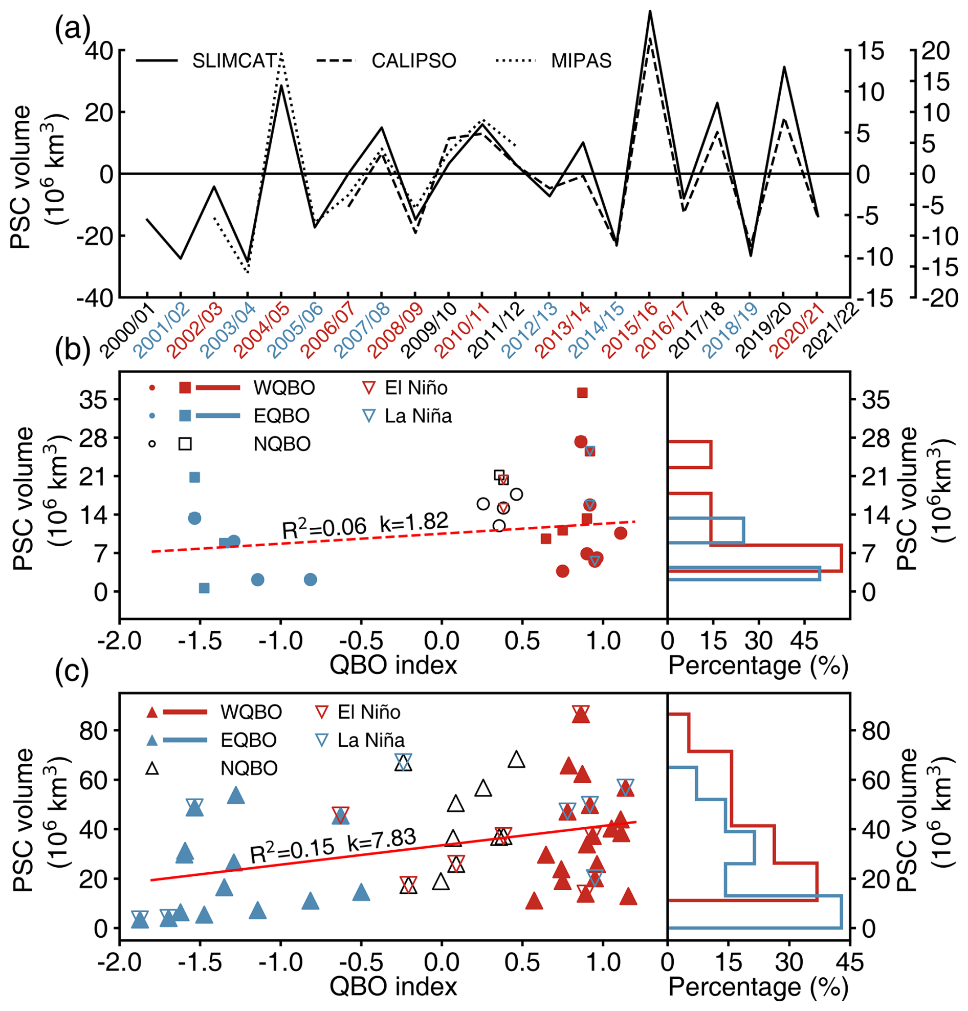
Figure 1 (a) Interannual variation of Arctic PSC volume (December–March mean) anomalies observed by CALIPSO and MIPAS and simulated by SLIMCAT. In the horizontal axis, blue and red labels indicate EQBO and WQBO winters, respectively. (b, c) Arctic PSC volume (December–March mean) plotted against the QBO index in December (left) from (b) CALIPSO and MIPAS observations and (c) SLIMCAT simulations. Triangles represent the PSC volume simulated by SLIMCAT from 1980 to 2022, circles represent the PSC volume observed by CALIPSO from 2007 to 2021, and squares represent the PSC volume observed by MIPAS from 2003 to 2012. Blue markers and red markers represent the PSC volume during EQBO and WQBO, respectively. In addition, red and blue downward-pointing triangles denote El Niño and La Niña winters, respectively. The red lines show the linear regression of the QBO index and the PSC volume for SLIMCAT and CALIPSO, respectively, with slopes (k) and coefficients of determination (R²) labeled. The solid line is statistically significant at the 95 % confidence level, while the dashed line is not. The probability distribution functions (PDF) of the PSC volume for the two QBO phases are shown on the right in (b) for CALIPSO and (c) for SLIMCAT.

To investigate the relationship between the QBO and PSCs, composite analyses of PSCs are performed (WQBO minus EQBO). It is important to note that before performing the composite analysis on all variables, the linear trends of the variables were removed. However, our results indicate that the detrending has a minimal impact on the composite results. Figure 2 shows the differences in the Arctic PSC area during winter between the WQBO and EQBO phases derived from the CALIPSO observations and the SLIMCAT simulations. The CALIPSO observations show that during the WQBO phase, the PSC area in January and February on 400–600 K isentropic levels is significantly larger than during the EQBO phase, whereas there is a non-significant negative area anomaly in mid-December. The differences in PSC area derived from SLIMCAT for the same periods are shown in Fig. 2b. Although the differences in the SLIMCAT PSC area are larger than those observed by CALIPSO, the simulations successfully reproduce the temporal and spatial distribution of the anomalies, such as the negative area anomaly in mid-December and the maximum positive anomaly on ∼ 500 K in January. The greater differences in SLIMCAT PSC area between the WQBO and EQBO phases primarily result from SLIMCAT simulating larger PSC areas than CALIPSO observations, likely due to CALIPSO's higher detection threshold (Li et al., 2024). We then analyze a longer dataset derived from SLIMCAT simulations from 1979–2022 (Fig. 2c). With increasing sample size, significant regions markedly increase. Furthermore, the negative area anomaly in mid-December shifts to a positive anomaly, although these positive anomalies are not significant, possibly due to the influence of negative anomalies in the 2006–2021 period. In contrast, the significance of the mean anomalies in December increases, as can be seen in the right panel of Fig. 2c. Furthermore, the maximum positive anomaly appears in January on ∼ 500 K isentropic level, and the height of the maximum anomaly gradually decreases from December to February, which is consistent with the climatological characteristics of the PSC area (Pitts et al., 2018; Li et al., 2024). These results confirm that the December QBO phase can significantly influence the PSC area in winter, with consistently larger areas observed during the WQBO phases compared to the EQBO phase.

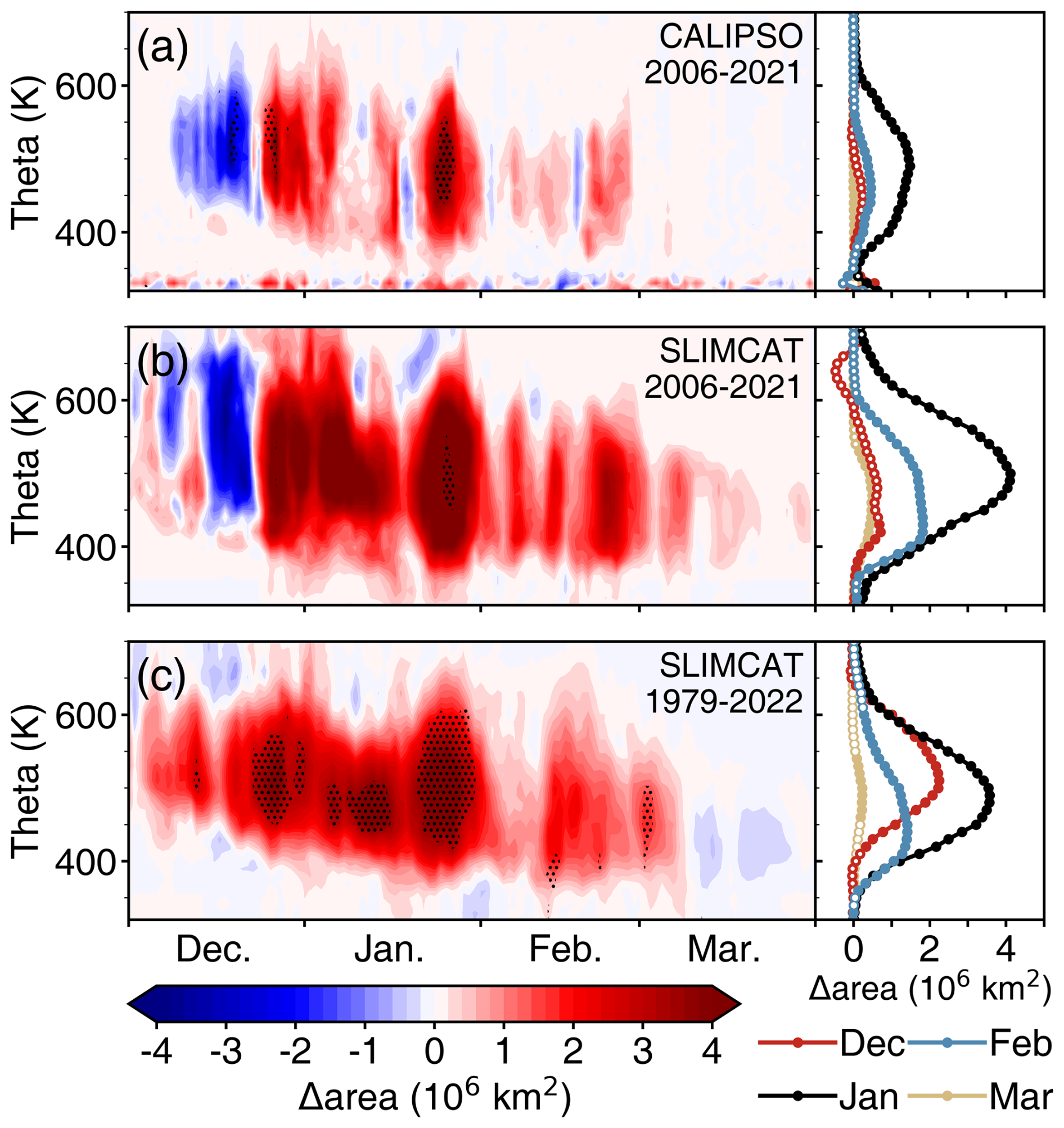
Figure 2 Differences in Arctic PSC area between the WQBO and EQBO phases, with variation over time on the left panel and monthly averages on the right panel, derived from (a) CALIPSO observations from 2006–2021, and SLIMCAT simulations from (b) 2006–2021 and (c) 1979–2022. Black dotted regions in the left panels and solid filled symbols in the right panels indicate the differences in PSC area are statistically significant at the 95 % confidence level according to the Student's t-test.

We bin the CALIPSO PSC data into the SLIMCAT model grid, where the monthly mean CALIPSO PSC occurrence frequency is defined as the number of PSC observations in each month per grid point divided by the total number of observations. The SLIMCAT PSC occurrence frequency is defined as the number of PSC occurrences at a grid point within a month divided by the number of days in that month. Figure 3 presents the spatial distribution of the differences in PSC occurrence frequency on 500 K derived from the CALIPSO observations. During the WQBO phase, the Arctic PSC occurrence frequency shows an overall positive anomaly in winter (Fig. 3a), with a clear zonal asymmetry. The largest positive anomaly occurs over Greenland and the Barents Sea. The anomaly is largest in January, followed by December, and smallest in February. The spatial distribution of this anomaly may be related to the climatology of PSC occurrence frequency. According to Pitts et al. (2018), the monthly mean PSC occurrence frequency in the Arctic peaks in January, with a clear zonal asymmetry, and the highest frequency is centered over the Barents Sea, corresponding to the lowest geopotential height of the Arctic stratospheric vortex (Zhang et al., 2016). The zonal asymmetry in PSC occurrence frequency anomalies in Fig. 3 may also be influenced by QBO-induced shifts in the polar vortex position, which we discuss further below. In addition, due to the smaller sample size, especially at lower latitudes, banded areas of positive and negative anomalies similar to the CALIPSO satellite orbit are exhibited.

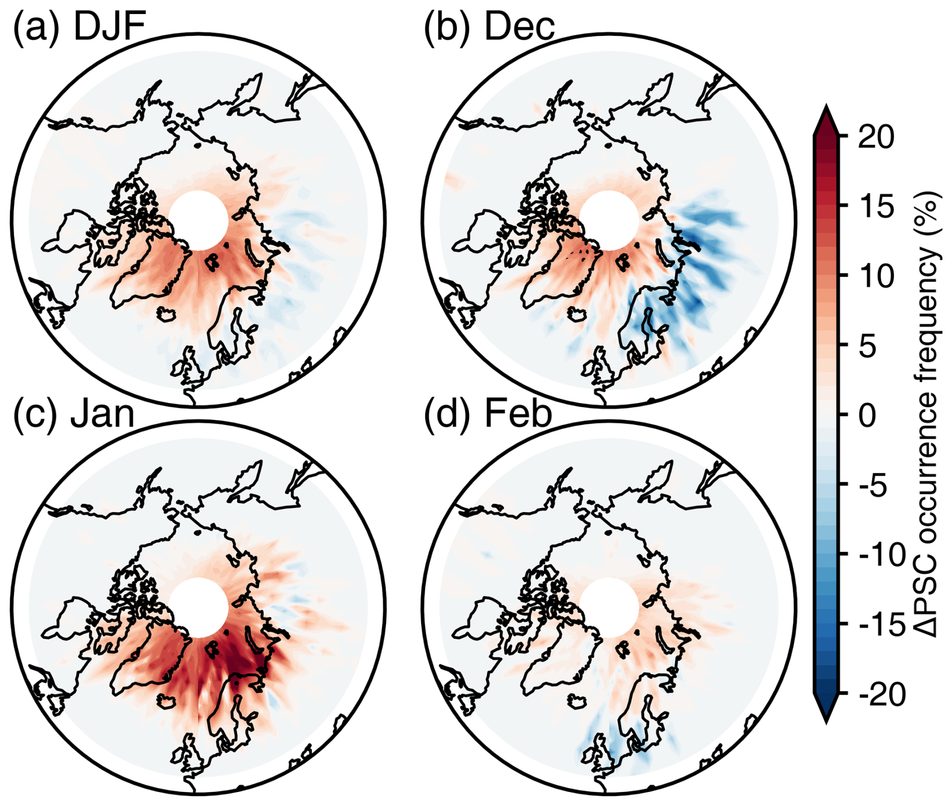
Figure 3 Differences in PSC occurrence frequency between the WQBO and EQBO phases on the 500 K isentropic level derived from the CALIPSO observations for the period 2006–2021 for (a) winter average (December to February), (b) December, (c) January, and (d) February. Black dotted regions indicate the differences in PSC occurrence frequency are statistically significant at the 95 % confidence level according to the Student's t-test.

Figure 4 presents the spatial distribution of the differences in the PSC occurrence frequency between the WQBO and EQBO phases from 1979 to 2022, as simulated by SLIMCAT. Compared to the CALIPSO results (Fig. 3), the increased sample size from SLIMCAT simulations leads to a larger anomalous region being statistically significant. In addition, the differences in SLIMCAT PSC occurrence frequency between the WQBO and EQBO phases are greater than those in CALIPSO PSC. Similar to the CALIPSO results, SLIMCAT simulations show notable positive anomalies during the WQBO phase compared to the EQBO phase, which also shows a zonal asymmetric structure. Furthermore, the zonal asymmetry appears to be more pronounced in December and February than in January. The non-significant negative anomalies over northern Eurasia are observed in December and February (Fig. 4b and d), which is also present in the CALIPSO observations (Fig. 3b). Zhang et al. (2019) suggested that during the WQBO phase, the NH polar vortex tends to shift towards North America and away from Eurasia during winter, compared to the EQBO phase. This shift may affect the distribution of PSCs, resulting in a reduction over Eurasia. However, this negative anomaly does not occur in January, probably due to a less pronounced polar vortex shift associated with the QBO. Overall, during the WQBO phase, the Arctic winter shows a positive anomaly in PSC occurrence frequency, the centre of which is located between Greenland and the Barents Sea. Compared to the climatological maximum frequency of PSC occurrence (Li et al., 2024), this positive anomaly lies upstream (west) of the maximum occurrence frequency.

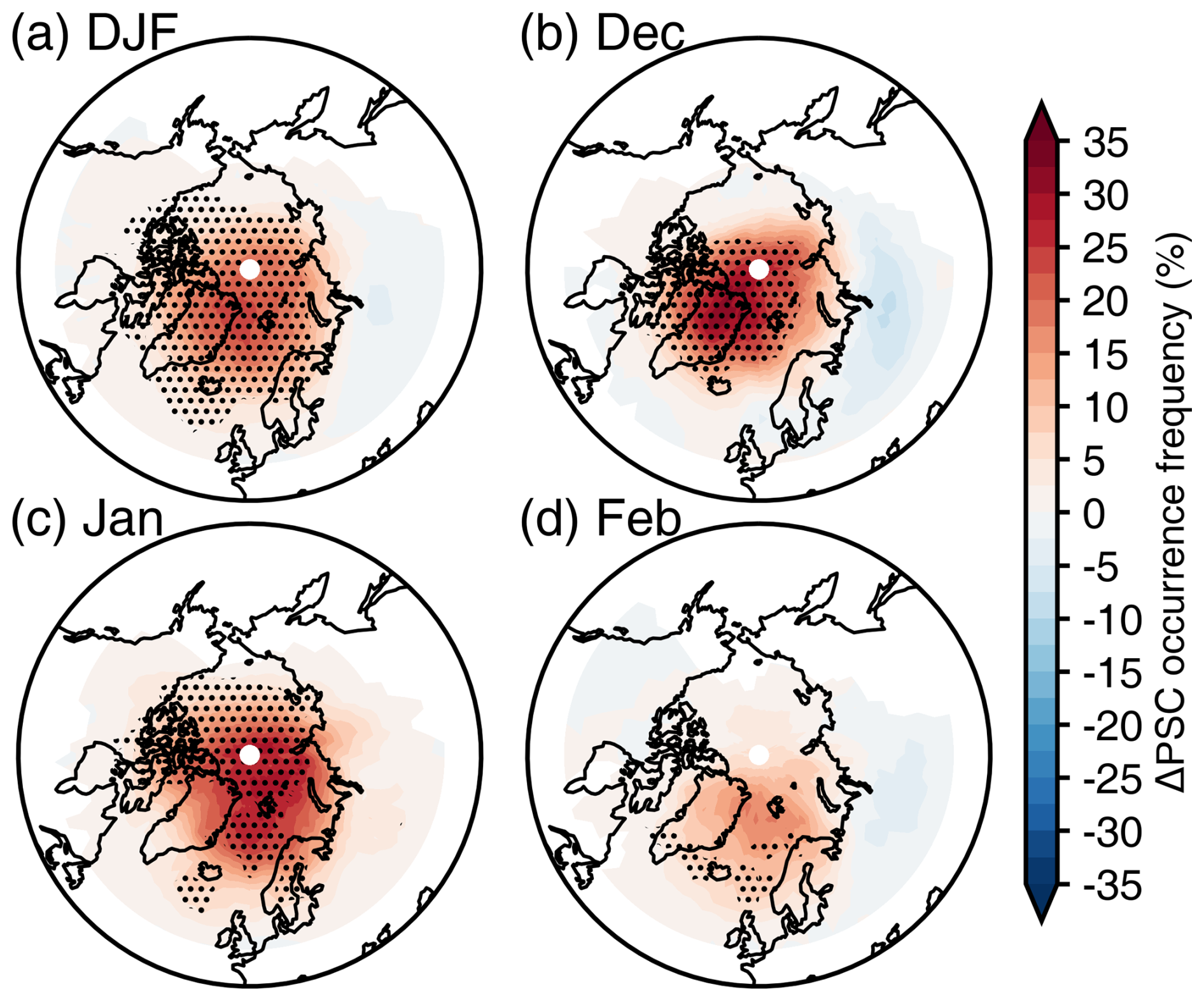
Figure 4 Same as Fig. 3 but derived from the SLIMCAT simulations for the period 1979–2022.

It is known that ENSO is another important factor influencing the Arctic stratospheric vortex in winter. During El Niño events, the Aleutian Low is deepened, planetary wave activity intensifies, and more planetary waves propagate into the mid- and high-latitudes of the NH stratosphere, thereby making the Arctic stratospheric polar vortex weaker and warmer than during La Niña events (Garfinkel and Hartmann, 2008; Salminen et al., 2020). Therefore, we should examine whether the conclusions that the QBO affects the PSC still hold after excluding the ENSO years. Figure 5 shows the differences in PSC occurrence frequency between the WQBO and EQBO phases, excluding years with strong ENSO. The results show similar patterns to Fig. 4, indicating that strong ENSO exclusion maintains the primary conclusions despite reducing the spatial significance extent due to reduced sample size.

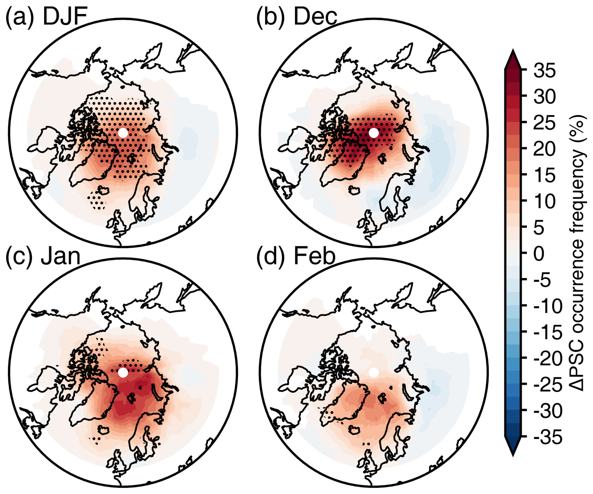
Figure 5 Differences in PSC occurrence frequency between the WQBO and EQBO phases on the 500 K isentropic level (excluding strong ENSO events) from SLIMCAT simulations for (a) winter average (December to February), (b) December, (c) January, and (d) February for the period 1979–2022. Black dotted regions indicate that the differences in PSC occurrence frequency are statistically significant at the 95 % confidence level according to the Student's t-test.

Figure 6 shows the zonal mean differences in PSC occurrence frequency during the WQBO and EQBO phases derived from the SLIMCAT simulations. Consistent with the result from Zhang et al. (2021), which reports differences in the number of days with temperatures below 195 K, PSC occurrence frequencies are higher during the WQBO phase compared to the EQBO phase, especially in December and January. Furthermore, the seasonal variation of the differences in PSC occurrence frequency is consistent with the seasonal variation in PSC area differences shown in Fig. 2, with the altitude of maximum difference progressively decreasing from December to February. Overall, in Fig. 6a, the differences in PSC occurrence frequency peaks near 500 K, with positive anomalies exceeding 10 % north of 75° N.

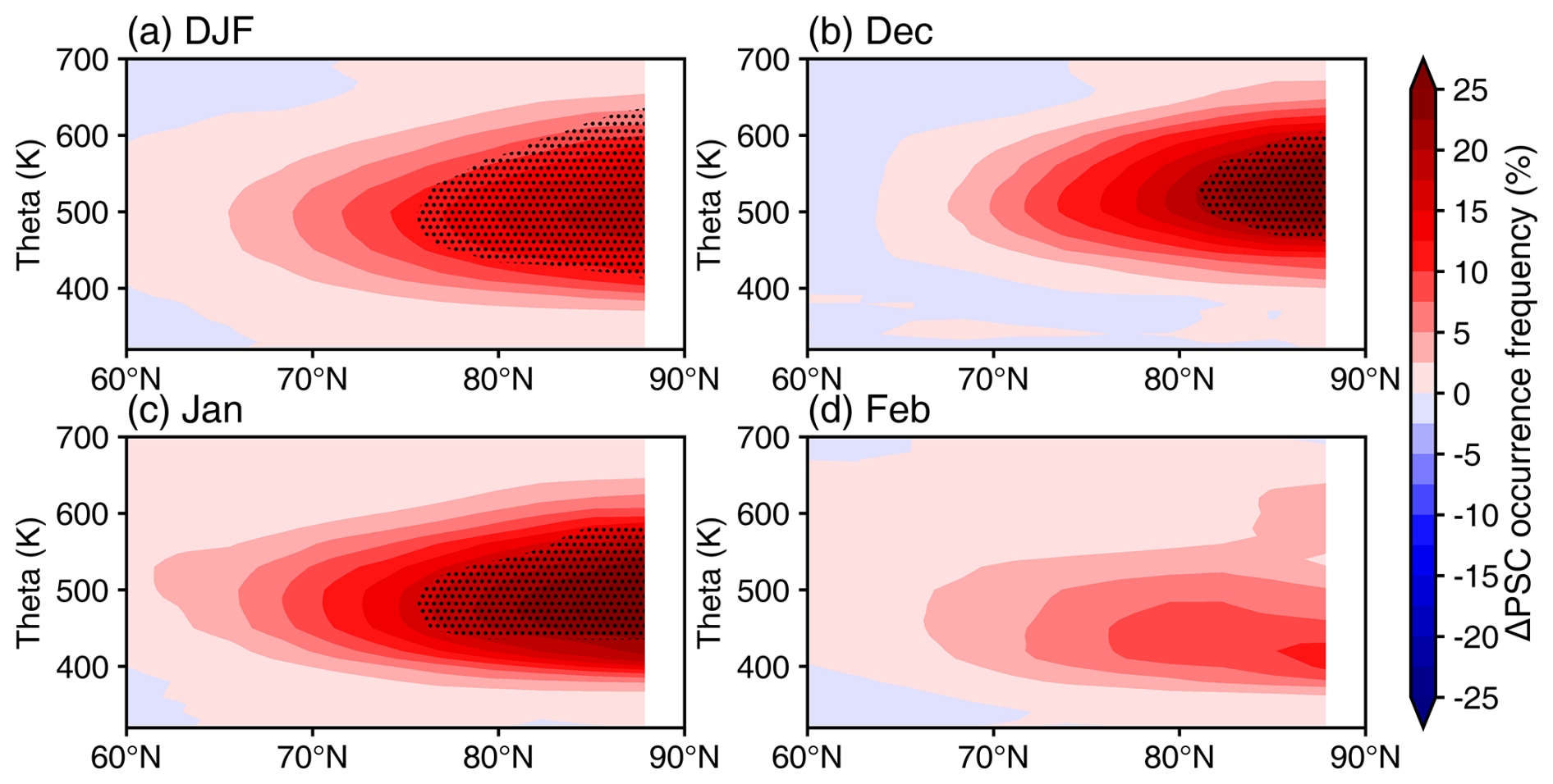
Figure 6 Differences in zonal-mean PSC occurrence frequency between the WQBO and EQBO derived from the SLIMCAT simulations for the period 1979–2022 for (a) winter average (December to February), (b) December, (c) January, and (d) February. Black dotted regions indicate that the differences in PSC occurrence frequency are statistically significant at the 95 % confidence level according to the Student's t-test.

3.2 How the QBO influences the Arctic PSC area

The above analyses reveal that the tropical QBO can significantly influence the Arctic PSC occurrence. During the WQBO phase, the Arctic PSCs have a larger coverage area and higher occurrence frequency, which may contribute to an increase in Arctic stratospheric ozone depletion. In addition, as mentioned in the introduction, the QBO may influence Arctic PSC formation through modulating temperature, H₂O, and HNO₃. However, it is unclear how QBO-induced changes in these factors affect PSC. The underlying mechanisms by which the QBO influences Arctic PSC are now discussed.

Figure 7 presents the climatological temperature and the composite differences in temperature between the WQBO and EQBO phases. The climatological temperature exhibits a clear zonal asymmetry, with the lowest temperatures biased towards the Eurasian continent, especially near the Barents Sea. This asymmetry aligns with the favored location of the recent Arctic vortex climatology (Zhang et al., 2016; Wang et al., 2022). Significant negative temperature anomalies are observed in most of the Arctic regions between the WQBO and EQBO phases, consistent with previous studies (Holton and Tan, 1980, 1982; Zhang et al., 2019). Furthermore, the temperature anomalies associated with the QBO show a distinct zonal asymmetry, with the centre of the anomalies biased towards North America. During the WQBO phase, the polar vortex is shifted towards North America, contributing to this asymmetry (Zhang et al., 2019). It is important to note that the asymmetry of the negative temperature anomaly is more pronounced in December and February, while it is relatively weaker in January.

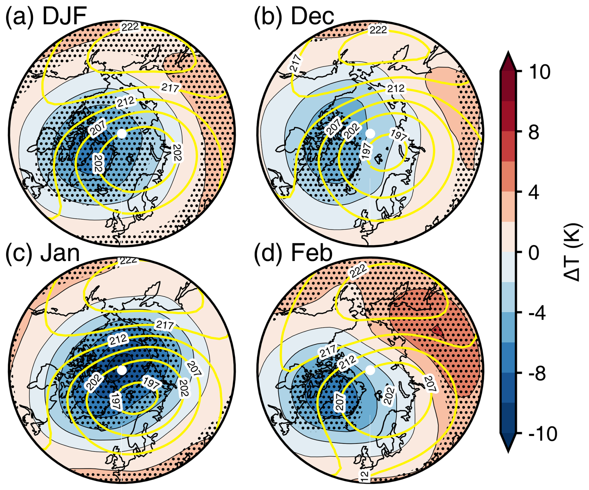
Figure 7 Climatological temperature (yellow contours) and the differences in temperature between the WQBO and EQBO phases on the 500 K isentropic level for the period 1979–2022 (shadings, WQBO–EQBO) derived from ERA5 data for (a) winter average (December to February), (b) December, (c) January, and (d) February. Black dotted regions indicate the differences in temperature are statistically significant at the 95 % confidence level according to the Student's t-test.

However, the negative temperature anomalies do not coincide well with the positive PSC occurrence anomalies, with the negative temperature anomalies located to the west of the positive PSC occurrence anomalies (Fig. 4). This is because PSC formation requires the ambient temperature to be sufficiently lower than the existence temperature (about 195 K; Tritscher et al., 2021). Only the QBO-induced Arctic cooling, occurring over the climatological cold centre, could lead to increased PSC occurrence. Therefore, the positive PSC anomalies are located near the climatological cold centre and appear to the east of the negative temperature anomalies.

In addition to the temperature, sufficient concentrations of H₂O and HNO₃ are critical for PSC formation (Li et al., 2024). Figure 8 shows the differences in H₂O and HNO₃ concentrations between the WQBO and EQBO phases observed by MLS and simulated by SLIMCAT over the Arctic (60–82° N). Both the MLS observations (Fig. 8a) and the SLIMCAT simulation (Fig. 8c) show positive H₂O anomalies above the 450 K isentropic level, with the maximum anomaly occurring in January and approaching ∼ 0.3 ppmv on the 650 K isentropic level. The altitude of the maximum positive anomaly of H₂O decreases with time similar to the decrease in the maximum positive anomaly of the PSC area, which may be related to the downward shift of the coldest centre of the polar vortex with time (Coy et al., 1997; Lawrence et al., 2018). In addition, SLIMCAT well reproduces the negative anomaly HNO₃ on 400–500 K, while the negative anomaly is smaller in December and January than in February and March.

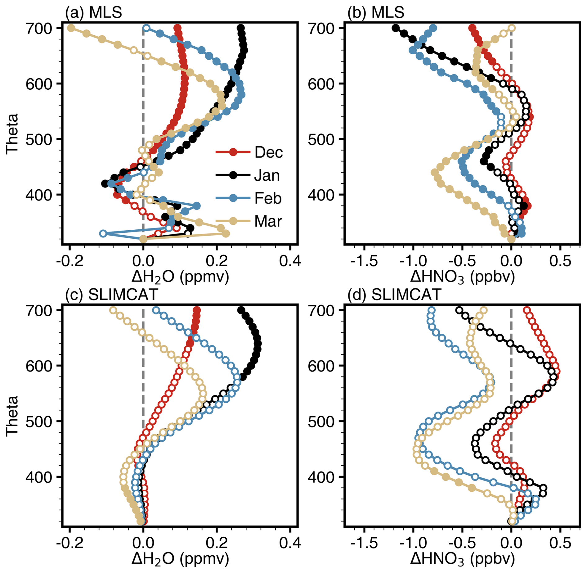
Figure 8 Differences in H₂O and HNO₃ averaged over 60–82° N between the WQBO and EQBO phases from (a, b) MLS observations and (c, d) SLIMCAT simulations for the period 2004–2021. Solid filled symbols indicate the differences are statistically significant at the 95 % confidence level according to the Student's t-test.

Stratospheric species are influenced by both dynamical and chemical processes. Due to the different chemical and physical properties of the different species, the factors affecting their concentrations also vary. Stratospheric H₂O has two primary sources: transport from the troposphere and the oxidation of methane (le Texier et al., 1988). Since stratospheric temperatures increase with altitude, H₂O produced by CH₄ oxidation reactions (primarily CH₄ + OH → CH₃ + H₂O) is more important in the older air in the upper stratosphere. In summer and autumn, H₂O produced by chemical reactions accounts for 50 % of the total stratospheric H₂O at the stratopause. In contrast, in the lower stratosphere, where temperatures are lower, CH₄ oxidation is weaker, and H₂O mainly originates from dynamical transport (Thölix et al., 2016). Therefore, chemical reactions are not the primary cause of the differences in H₂O between the WQBO and EQBO phases.

Hansen et al. (2013) provided an explanation for the positive H₂O anomalies during the WQBO phase, attributing these anomalies to dynamical transport processes. Specifically, they proposed that the vertical transport anomaly of the BD circulation induced by the QBO leads to an increase in H₂O. To explore the relationship between H₂O anomalies and BD circulation anomalies, Fig. 9 shows the time evolution of the H₂O anomalies and climatology and the vertical velocity anomalies of the BD circulation in the Arctic lower stratosphere. The H₂O concentration in the polar stratosphere increases with altitude, which is caused by the CH₄ oxidation (Grooß and Russell, 2005). If the BD circulation anomalies are the direct cause of the H₂O anomalies, the anomalous upward vertical velocity, corresponding to a weaker BD circulation, would transport less H₂O-rich air from the upper layers to the lower layers, resulting in a negative H₂O anomaly. Therefore, the BD circulation anomalies cannot account for the positive H₂O anomalies as seen in MLS and SLIMCAT.

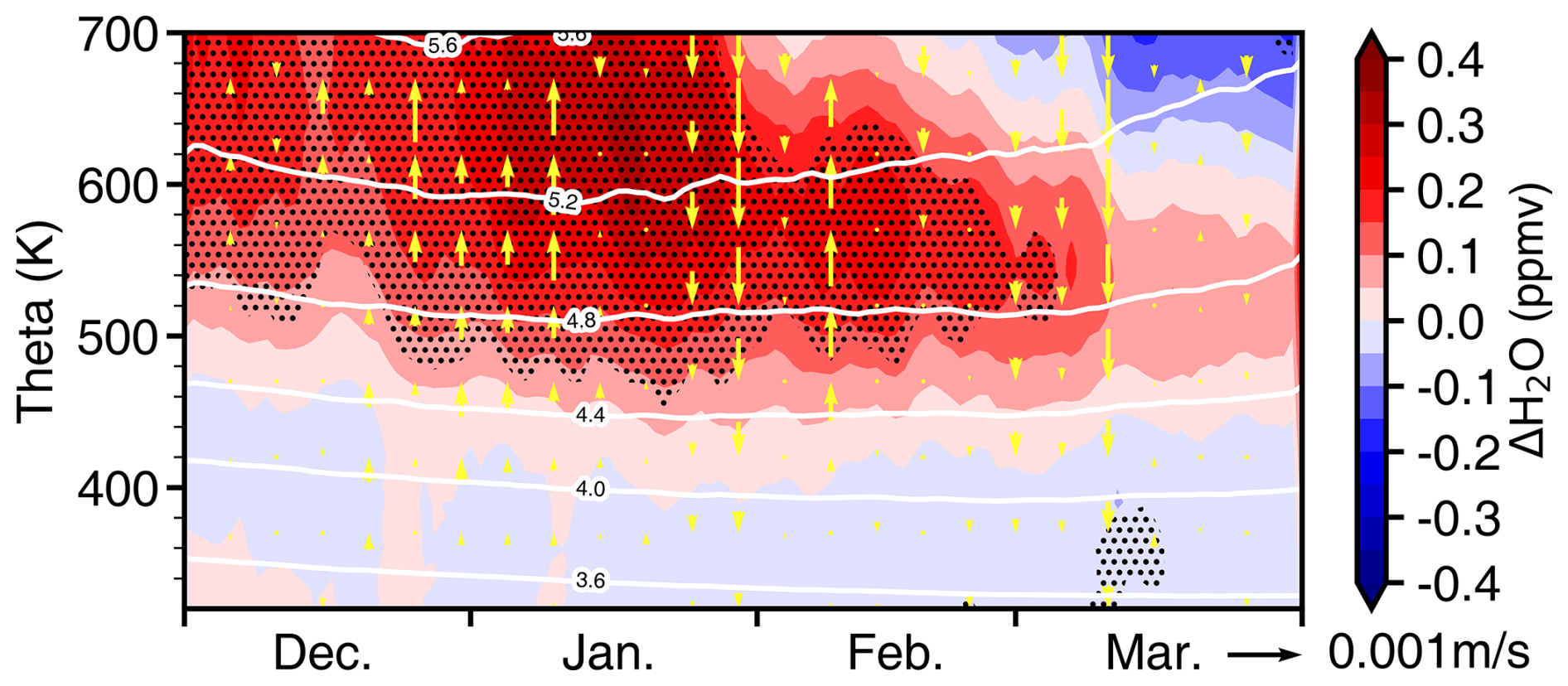
Figure 9 Differences in H₂O (shading) and vertical component of BD circulation (yellow arrows) over the Arctic between the WQBO and EQBO phases from SLIMCAT simulations for the period 1979–2022. The white contours are the climatological concentration of the H₂O. Black dotted regions indicate the differences in H₂O are statistically significant at the 95 % confidence level according to the Student's t-test.

Changes in tropopause temperature and permeability may also influence stratospheric H₂O. In the Arctic, the tropopause is typically located around the 320 K potential temperature level. However, we note that the positive H₂O anomalies observed and simulated in our study are mainly concentrated above the 450 K, with no significant positive H₂O anomaly signals detected on 320–450 K (Fig. 8a and c). Therefore, we consider that local processes at the tropopause are unlikely to be the primary drivers of the H₂O anomalies above the 450 K.

Another potential cause for the anomalies in Arctic stratospheric chemical species could be the stratospheric polar vortex. This isolates the polar air from that outside the vortex. Khosrawi et al. (2016) found a clear inverse correlation between H₂O and temperature in the Arctic lower stratosphere, suggesting a high H₂O concentration in the Arctic lower stratosphere under a strong polar vortex. Pan et al. (2002) found that decreased amounts of tracers can be transported outside the vortex during strong polar vortex conditions compared to weak polar vortex conditions. In the lower stratosphere, H₂O concentrations are higher in the polar regions than in the mid-latitudes at the same altitude (Randel et al., 2001; Jiang et al., 2015), which is related to the downwelling branch of the BD circulation in the polar regions and the upwelling branch in the tropics (Morrey and Harwood, 1998). Therefore, a strong polar vortex may prevent the transport of high-moisture air at high latitudes to mid-latitudes, leading to increased H₂O concentrations within the vortex. Here, the zonal winds averaged over 60–65° N on the 500 K isentropic level are used to define the strength of the Arctic polar vortex. The relationship between polar vortex strength and H₂O concentration across different latitude bands is shown in Fig. 10a and c. Given the overall increasing trend in stratospheric H₂O concentration driven by global warming and increased methane emissions (Nedoluha et al., 1998; Oltmans et al., 2000; Dessler et al., 2013; Smalley et al., 2017), the monthly mean H₂O has been detrended before analysis. Both the MLS observation and the SLIMCAT simulation reveal a strong positive correlation between the Arctic H₂O concentration and the polar vortex strength, with correlation coefficients of 0.84 for the observations and 0.74 for the simulation. In contrast, the H₂O concentration in the mid-latitudes decreases as the polar vortex strengthens. The relatively slow decrease of H₂O in the mid-latitudes can be explained by the larger volume of air at the same latitude range, which makes it less susceptible to the influence of polar H₂O transport. The opposite evolution of H₂O inside and outside the polar vortex suggests that a stronger vortex suppresses the transport of H₂O from the polar region to mid-latitudes. Therefore, a stronger polar vortex induced by the WQBO isolates high concentrations of H₂O within the polar region, resulting in higher H₂O concentrations compared to the EQBO.

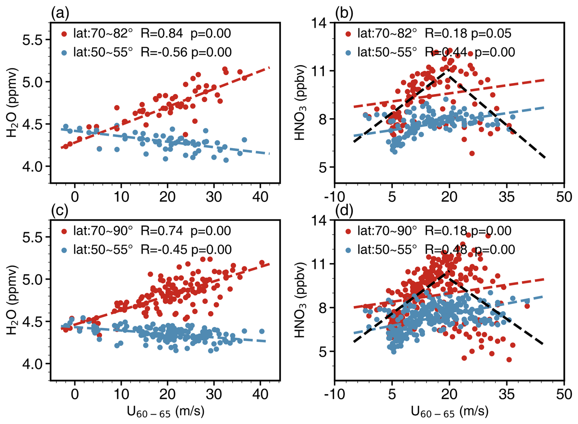
Figure 10 Relationship between (a, c) H₂O and (b, d) HNO₃ and the zonal mean wind between 60 and 65° N on the 500 K isentropic level. Data from (a, b) MLS observations (2004–2022) and (c, d) SLIMCAT simulation (1979–2022) for the period (a, c) December to February and (b, d) September to February. Red represents high-latitude regions (MLS: 70–82° N, SLIMCAT: 70–90° N), and blue represents mid-latitude regions (50–55° N). Dashed lines represent linear fits, with R denoting the correlation coefficient. The black dashed line provides a segmented fit before and after 20 m s⁻¹ at high latitudes. Values of p<0.05 are considered statistically significant.

Since the change in stratospheric HNO₃ from December to February is relatively small, we display the relationship between HNO₃ from MLS and SLIMCAT and polar vortex strength from September to February (Fig. 10b and d). Overall, HNO₃ concentrations in the mid- and high-latitudes of the NH stratosphere increase with polar vortex strength. The correlation between HNO₃ and polar vortex strength is stronger in the mid-latitudes (with coefficients of 0.44 for observations and 0.48 for simulations) and is statistically significant, while the correlation is weaker in the high-latitudes (coefficients of 0.18 for observations and simulations), with weaker significance. Notably, the relationship between HNO₃ concentrations and polar vortex strength in the high-latitude stratosphere shows two distinct trends around wind speeds of 20 m s⁻¹. When wind speeds are below 20 m s⁻¹, HNO₃ concentrations increase with wind speed, but above 20 m s⁻¹, HNO₃ concentrations decrease.

HNO₃ is an important reservoir molecule for stratospheric reactive nitrogen (NO_y), produced by the oxidation of NO_x (NO₂ + OH + M → HNO₃ + M). However, under solar radiation, HNO₃ is destroyed through photolysis (HNO₃ + hv → OH + NO₂) and reactions with OH (HNO₃ + OH → H₂O + NO₃) (Keys et al., 1993), leading to lower concentrations in the Arctic stratosphere in summer. As solar radiation decreases in autumn, the stratospheric polar vortex begins to form, and the reduction in photolysis and the heterogeneous chemical reactions on background aerosols cause HNO₃ concentrations to increase gradually (Solomon and Keys, 1992; Keys et al., 1993). Therefore, as the strength of the polar vortex increases, HNO₃ concentrations increase in the mid- and high-latitude regions of the NH stratosphere. However, once wind speeds reach a certain level and the polar vortex becomes sufficiently strong and isolated, temperatures can become low enough for NAT to form. If a sufficient amount of NAT has formed, denitrification occurs within the polar vortex due to the NAT sedimentation, leading to a decrease in HNO₃ concentrations. This explains the observed decrease in HNO₃ concentrations at wind speeds above 20 m s⁻¹, as shown in Fig. 10b and d. During winter and early spring, Arctic temperatures are sufficiently low for denitrification to occur. Therefore, the lower temperatures during the WQBO phase result in lower HNO₃ concentrations compared to the EQBO phase (Fig. 8b and d).

Both H₂O and HNO₃ concentrations are influenced by PSC sedimentation. When the polar vortex is strong enough, both H₂O and HNO₃ concentrations decrease. It is important to note that different types of PSCs have different effects on stratospheric chemicals. NAT sedimentation primarily affects HNO₃ concentrations, while ice PSC sedimentation primarily affects H₂O concentrations. The contrasting thermal climatologies between the Arctic and Antarctic lead to fundamental differences in PSC composition, with ice PSCs constituting about 25 % of Antarctic PSCs but less than 5 % of Arctic PSCs (Pitts et al., 2018). As a result, ice PSC-related dehydration occurs annually in the Antarctic but rarely in the Arctic (Khaykin et al., 2013). Since NAT accounts for approximately 40 % of PSCs in the Antarctic and up to 60 % in the Arctic, significant denitrification can occur in both polar regions. Due to the dominance of NAT and the scarcity of ice particles in Arctic PSCs, the effects of the QBO on Arctic stratospheric HNO₃ and H₂O are markedly different.

As mentioned above, the WQBO phase tends to lower the Arctic temperatures (Fig. 7), reduce HNO₃ concentrations, and increase the H₂O concentrations (Fig. 8). The lower temperatures and higher H₂O concentrations are favourable for PSC formation, while the lower HNO₃ concentrations are unfavourable (Hanson and Mauersberger, 1988). However, their relative contributions remain unclear. To address this issue, we perform sensitivity analyses in which the temperature, H₂O, and HNO₃ are adjusted by adding or subtracting 50 % of the differences between the WQBO and EQBO phases. It is important to note that we did not adjust temperature, H₂O, and HNO₃ during the model runs, but instead made these adjustments during the offline diagnosis of the PSCs. Our adjustment strategy aims to reduce the PSC area during the WQBO phase and increase it during the EQBO phase, to investigate the main factors influencing Arctic PSCs by changing temperature, H₂O, and HNO₃. Table 2 provides the descriptions of the six sensitivity analyses.

Table 2 Description of the sensitivity analyses, where Δ represents the differences between the WQBO and EQBO phases.

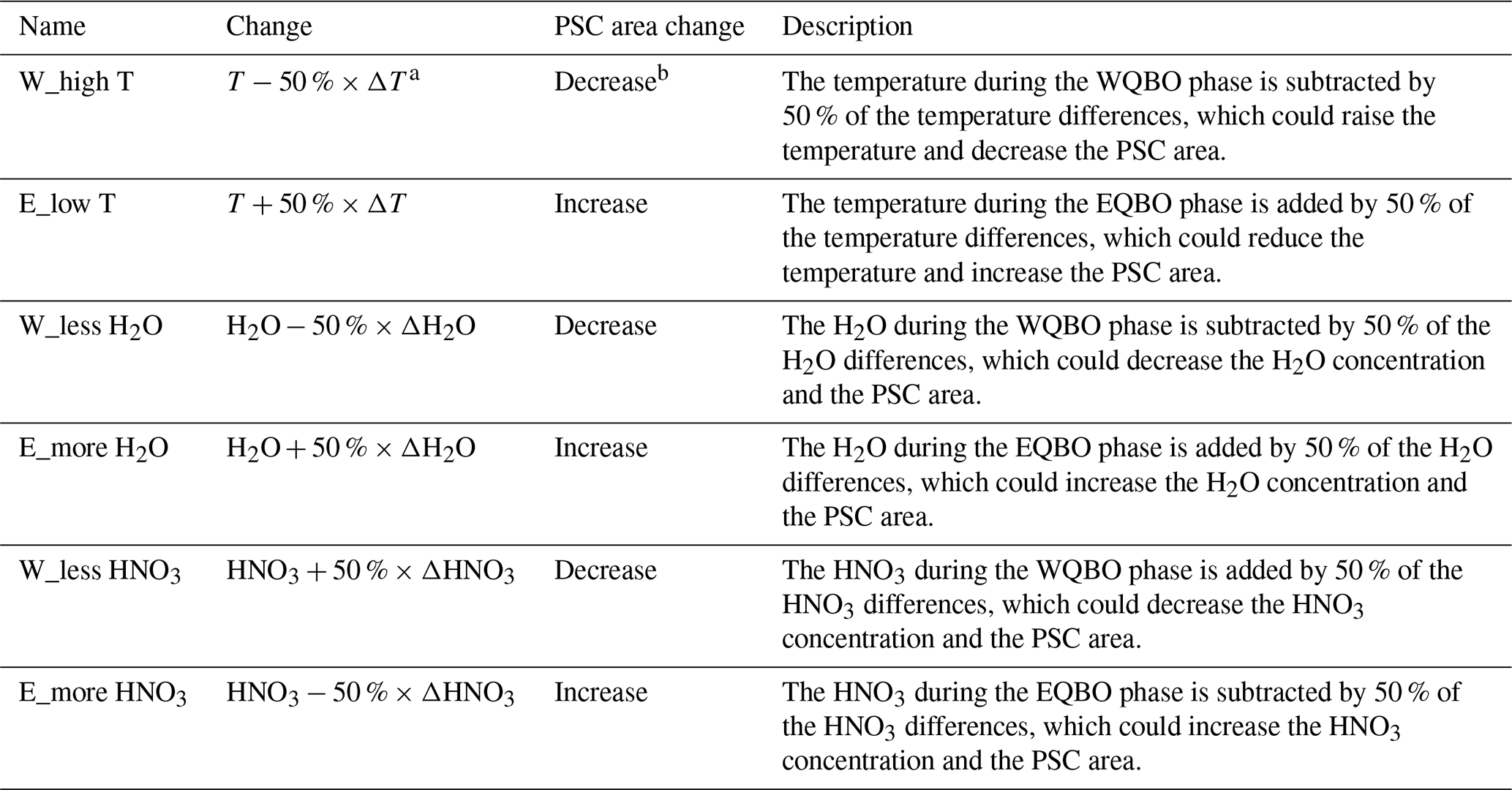
Note: ^a According to the above composite analyses, temperature and HNO₃ show negative anomalies and H₂O shows positive anomalies during the WQBO phase. ^b Higher temperatures, less H₂O and HNO₃ are unfavourable for PSC formation.

Note that the temperature variation induced by the QBO accounts for most of the changes in the PSC areas (Fig. 11a–d). In particular, during the WQBO phase, when the temperature is subtracted by 50 % of the differences between the WQBO and EQBO phases, that means warmer than the original temperature, the PSC areas decrease and approach those during the EQBO phase. In contrast, during the EQBO phase, when the temperature is added by 50 % of the differences between the WQBO and EQBO phases, that means colder, the PSC area increases slightly. This suggests that PSC formation is more sensitive to temperature variations during the WQBO phase. Since Arctic temperatures are concentrated around the PSC formation threshold (Fig. 7), PSCs are highly sensitive to temperature changes, and even small changes in temperature will result in significant variations in PSC. QBO-induced changes in H₂O and HNO₃ lead to only small changes in PSC. During the WQBO phase, when the H₂O decreases by 50 % of the difference, the PSC area becomes smaller, although the magnitude of the change is relatively small (Fig. 11e–h). QBO-induced HNO₃ changes affect the PSC in late winter and early spring (Fig. 11k–l). During the WQBO phase, lower Arctic temperatures lead to stronger denitrification, resulting in less HNO₃ participating in PSC formation. These results show that it is important to simulate the NAT sedimentation process in the model accurately.

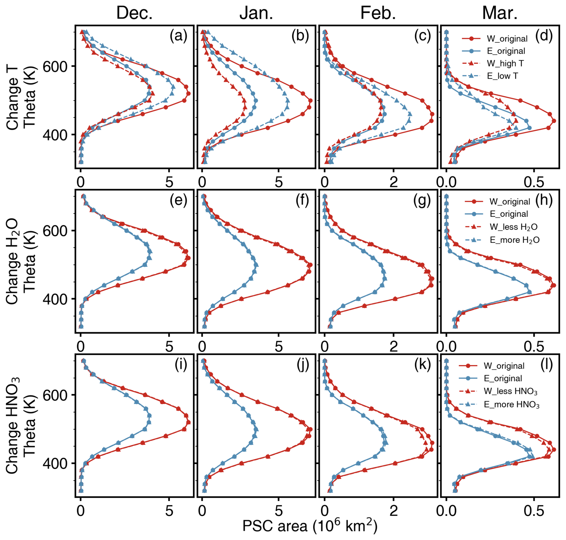
Figure 11 PSC area from December to March during the WQBO (red) and EQBO (blue) phases. The first, second, and third rows show the results from sensitivity analyses with imposed temperature, H₂O, and HNO₃ changes. Solid lines represent results before the changes, and dashed lines represent results after the changes.

4 Discussion and conclusions

Using CALIPSO observations data and the SLIMCAT simulations, we analyze the impact of the QBO on the occurrence of Arctic PSCs. The results show that as the QBO index increases, the volume of Arctic PSCs gradually increases, indicating that the winter PSC volume is significantly larger during the WQBO phase than during the EQBO phase. Both CALIPSO observation and SLIMCAT simulation show maximum positive anomaly occurring near the 500 K isentropic level in January. From December to February, the center of the PSC anomaly gradually decreases in altitude. Compared to the SLIMCAT simulations for the same period (2006–2021), the CALIPSO PSC area anomalies between the WQBO and EQBO are smaller, while SLIMCAT reproduces the distribution of these anomalies accurately. It is important to note that when the sample size is small, composite analysis results may be influenced by individual extreme events. For example, the negative anomaly in the PSC area derived from CALIPSO in December may have been driven by a few specific years, which is contrary to the theoretical expectations. To address this issue, we used SLIMCAT simulations for the period 1979–2022 to reduce the impact of individual extreme events on the composite results. The results show that with the extension of the simulation period, a positive anomaly consistent with theoretical expectations occurs in December, and the statistical significance of the composite analysis is improved.

Both CALIPSO observations and SLIMCAT simulations show a clear zonal asymmetry in the PSC occurrence frequency anomaly between the WQBO and EWBO phases on the 500 K isentropic level. During the WQBO phase, there is a positive anomaly in the occurrence frequency of Arctic winter PSCs, with the maximum positive anomaly located between Greenland and the Barents Sea. This region is close to the region of maximum PSC occurrence frequency (Li et al., 2024) and the location of the lowest geopotential height of the Arctic polar vortex (Zhang et al., 2016).

The QBO affects Arctic PSCs through its effects on stratospheric temperature, H₂O, and HNO₃. We have analyzed the temperature, H₂O, and HNO₃ anomalies induced by the QBO. Compared to the EQBO phase, there is a zonal asymmetry in the negative temperature anomaly in the Arctic stratosphere during the WQBO phase. The maximum negative anomaly is located upstream (west) of the climatological minimum temperature. MLS satellite observations and SLIMCAT simulations show a positive H₂O anomaly and a negative HNO₃ anomaly in the Arctic lower stratosphere during the WQBO phase. The positive H₂O anomaly is mainly due to the stronger polar vortex during the WQBO phase than during the EQBO phase, which prevents the transport of high-moisture air at high latitudes to the mid-latitudes, causing H₂O to accumulate inside the polar vortex. In contrast, the negative HNO₃ anomaly is primarily attributed to denitrification caused by the sedimentation of NAT particles. It is worth noting that ice PSCs can also sediment, leading to dehydration in the lower stratosphere. However, due to the high temperatures in the Arctic stratosphere, ice PSCs rarely form in the NH polar region (Tritscher et al., 2021), and thus dehydration events are rare.

Through six sensitivity analyses, we find that the temperature anomalies between the WQBO and EQBO phases are the primary cause of PSC anomalies. During the WQBO phase, PSCs are more sensitive to temperature changes, while H₂O anomalies have a smaller impact on PSCs. HNO₃ anomalies affect PSCs in late winter and early spring. It should be noted that the negative HNO₃ anomaly during the WQBO phase not only affects the formation of PSCs in late winter and early spring, but also prolongs the lifetime of active chlorine, thereby increasing ozone depletion. Feng et al. (2011) found that, compared to simulations of the 2004/2005 Arctic winter without denitrification, denitrification increased ozone depletion by about 30 %. This suggests that QBO-induced HNO₃ anomalies may also affect Arctic stratospheric ozone by affecting the lifetime of active chlorine.

The impact of the QBO on Arctic PSCs exhibits zonal asymmetry. Influenced by the QBO-induced displacement of the NH polar vortex, the centre of the negative temperature anomaly is located approximately 90° west of the climatological minimum temperature (Fig. 7). Temperature-sensitive PSCs tend to form in the region between the temperature minima and the negative anomaly centre, which is consistent with the results shown in Figs. 3 and 4. In addition, the shift of the polar vortex leads to positive temperature anomalies north of the Eurasian continent during the EQBO phase. However, because this positive anomaly centre is further away from the temperature minimum, it has little impact on PSC formation. As a result, the northern Eurasian continent has a relatively non-significant negative anomaly in PSC occurrence frequency.

Although our study provides evidence for the influence of QBO phases on Arctic PSC occurrence and associated stratospheric chemical composition changes, several limitations must be acknowledged. First, the SLIMCAT model used in this study is an offline chemical transport model driven by reanalysis data. Despite prescribing fixed ODS as well as climatological SAD and solar flux in the simulations, it is impossible to fully isolate the QBO signal from other factors such as ENSO, solar variability, and volcanic aerosols. Although composite analyses help to reveal QBO-related effects, the resulting anomalies may still contain contributions from other climate factors, which may contaminate the impact of QBO on Arctic PSC occurrence. Second, SLIMCAT does not include the chemical-radiative-dynamical coupling process. As an important trace gas in the stratosphere, H₂O not only affects chemical reactions but also contributes to the radiative cooling of the stratosphere (Bi et al., 2011). Forster and Shine (2002) showed that a 1 ppmv increase in stratospheric H₂O results in a 0.8 K decrease in the temperature of the tropical lower stratosphere, with a more pronounced cooling of 1.4 K at high latitudes. Similarly, Tian et al. (2009) found that a 2 ppmv increase in H₂O causes a temperature decrease of more than 4 K in the stratosphere at high latitudes. In particular, due to the high sensitivity of PSC formation to temperature, the indirect effects of H₂O on PSCs by influencing temperature may be comparable to its direct effects. In our sensitivity analyses, we only consider the direct effect of H₂O changes on PSCs, without accounting for the indirect impact of radiative cooling induced by H₂O anomalies. This omission may lead to an underestimation of the QBO's impact on the Arctic PSC area in Fig. 11e–h. Finally, in SLIMCAT, denitrification and dehydration are implemented by assuming fixed sedimentation velocities for NAT and ice particles based on prescribed particle radii or number densities. This simplified scheme still shows discrepancies in H₂O and HNO₃ compared to MLS observations. Incorporating more complex microphysical schemes, such as the DLAPSE, which incorporates the nucleation, growth, and settlement processes of PSC particles, could improve the simulation of the spatial distribution of H₂O and HNO₃. However, detailed microphysical schemes are too expensive for long-term simulations. Moreover, as PSC formation is primarily modulated by temperature, the relationship between QBO and PSCs established in this study remains robust.

This study investigates the impact of the QBO on Arctic PSC occurrence. Given the increasing frequency of QBO disruptions and the weakening of QBO amplitude in the lower stratosphere due to climate change (Diallo et al., 2022; Wang et al., 2023), understanding how the QBO influences PSCs is crucial for predicting future changes in Arctic stratospheric chemical ozone depletion. A future weakening of the QBO amplitude (Diallo et al., 2022) may reduce its modulation of the polar vortex and temperature in the Arctic stratosphere, thereby reducing its effect on PSC variability.