Machine learning interatomic potentials with accurate long-range interactions for molecular dynamics collision simulations of atmospherically-relevant molecules

Molecular collisions and subsequent clustering events are fundamental to atmospheric cluster formation. Accurately modeling these processes requires interatomic potentials that simultaneously capture the long-range forces governing collision kinetics and the short-range quantum effects driving reactivity. In this work, we evaluate the AIMNet2 and PaiNN machine learning architectures trained on GFN1-xTB and ωB97X-3c quantum chemical data for molecular collisions involving sulfuric acid.

The models exhibit low mean absolute errors in energies and forces and accurately reproduce potentials of mean force relative to the GFN1-xTB reference. However, discrepancies are observed for the collision dynamics. While AIMNet2 accurately reproduces reference collision rate coefficients across all systems, PaiNN underestimates the rate coefficient for the charged sulfuric acid–bisulfate system by ∼ 50 %. This error originates from the model's local atomic environment approximation, which neglects the strong long-range attractive forces at large intermolecular distances. Simulations with the OPLS-AA classical force field demonstrate that simple fixed partial charges are sufficient to describe these interactions.

Comparing models trained on GFN1-xTB and ωB97X-3c data reveals that while increasing the level of electronic structure theory significantly alters the potential energy surface in the short-range binding region, it generally has less impact on the long-range shoulder and the resulting collision rate coefficients.

Our results highlight that while local equivariant models like PaiNN offer exceptional accuracy for thermodynamics, correctly simulating collision kinetics in systems with strong long-range interactions requires models that explicitly account for forces beyond the local environment, such as AIMNet2.

1 Introduction

Atmospheric aerosol particles influence the climate by affecting cloud formation and scattering sunlight (Haywood and Boucher, 2000), while also posing risks to human health via inhalation (Gan et al., 2013). According to the latest Intergovernmental Panel on Climate Change (IPCC) assessment report, interactions between aerosols and clouds remain one of the largest sources of uncertainty in current global climate models (Chen et al., 2021). A major contributor to this uncertainty is the difficulty of accurately modeling the earliest stages of particle formation (Tröstl et al., 2016).

Most atmospheric aerosol particles form through a gas-to-particle conversion process called new particle formation (NPF), in which gas-phase molecules collide and stick together to form clusters (Kulmala et al., 2013). These clusters then grow further through condensation and coagulation (Zhang et al., 2012). The earliest stages of this formation are inherently dynamic: molecules approach each other under the influence of long-range attractive forces (e.g., van der Waals or electrostatic interactions), then rearrange and relax to accommodate one another while forming a thermodynamically stable cluster.

To capture the dynamic nature of these initial steps, researchers increasingly rely on atomistic molecular dynamics (MD) simulations. These simulations provide a fully atomistic description and offer insight into the molecular-level dynamics governing collisions and the formation of stable clusters. However, accurately capturing the necessary physics at a reasonable computational cost remains challenging. The quality of MD simulations is in large part determined by the level of theory at which the interaction potential between the nuclei in the system is obtained. An ideal interatomic potential for particle formation MD must satisfy three competing requirements: it must accurately capture long-range attractive forces to model how molecules initially approach; it must describe short-range quantum effects, such as chemical reactions, to model cluster stabilization; and it must be computationally efficient enough to sample a statistically significant number of events.

These effects include chemical reactions like proton transfers, which play a critical role in stabilizing atmospheric clusters. While semi-empirical quantum chemistry methods such as GFN1-xTB (Grimme et al., 2017) can model bond-breaking, they can exhibit significant errors for complex hydrogen-bonded systems, including quantitative inaccuracies in binding energies (Neefjes et al., 2026) and qualitative misidentifications of lowest-energy cluster configurations (Kubečka et al., 2019). Higher levels of theory, such as the DFT composite method ωB97X-3c (Müller et al., 2023), offer the necessary short- and long-range accuracy, but their computational cost makes even short MD simulations of small systems prohibitively expensive. Thus, neither classical nor conventional ab initio methods fully satisfy the requirements for large-scale cluster formation MD.

Recently, several machine learning (ML) architectures have been developed to construct accurate interatomic potentials for molecular systems. These machine learning interatomic potentials (MLIPs) offer a potential solution to this tradeoff, promising to reproduce the accuracy of high-level quantum theory at a reasonable computational cost. For instance, the polarizable atom interaction neural network (PaiNN) is an equivariant message-passing neural network capable of accelerating MD simulations while maintaining accuracy comparable to its reference training data (Schütt et al., 2021; Kubečka et al., 2024). Similarly, the second-generation atoms-in-molecules neural network (AIMNet2) has demonstrated high predictive accuracy across a wide range of molecular systems with remarkable efficiency, enabling simulations of systems containing up to 10⁵ atoms (Anstine et al., 2025).

However, MLIPs often rely on a local atomic environment approximation, in which the model encodes the environment around each atom up to a user-defined cutoff radius. This approximation improves transferability and computational efficiency but inherently limits the model to short-range interactions. The PaiNN model addresses this through a message-passing framework, where atoms exchange information with their neighbors via message and update blocks. Through multiple iterations, the effective interaction range grows, allowing atoms to indirectly access information from beyond the immediate cutoff. However, if all atoms in one subsystem (e.g., a molecule) lie beyond the cutoff radius of another, the interaction graph becomes disconnected. Consequently, no messages are exchanged, and the model treats the subsystems as non-interacting. AIMNet2 mitigates this by supplementing message passing with explicit long-range contributions. It predicts partial charges to model analytical Coulomb interactions and adds dispersion effects via the D3(BJ) correction scheme (Grimme et al., 2010, 2011).

The potential of MLIPs for atmospheric modeling has already been demonstrated by several recent studies that simulated the evolution of systems containing tens of particle-forming molecules to observe cluster formation dynamics (Jiang et al., 2022, 2023; Liu and Jiang, 2025). As the field increasingly adopts these methods for large-scale simulations, it is important to evaluate how well different model architectures capture long-range interactions alongside the necessary short-range accuracy and computational efficiency.

A rigorous metric for evaluating this long-range capability is the canonical collision rate coefficient. In cluster distribution dynamics models, such as the Atmospheric Cluster Dynamics Code (ACDC) (McGrath et al., 2012), cluster-forming collisions and cluster-removing evaporations are treated as independent processes, assuming that dissociation prior to thermalization from collisional excitation is negligible (Elm et al., 2020). This yields a pressure-independent collision rate coefficient, which represents the frequency of collisions per unit concentration. Traditionally, this coefficient is calculated using kinetic gas theory. In this framework, colliding partners are approximated as hard spheres, and intermolecular interactions are neglected entirely. While analytical approaches like the central field model can account for long-range forces, they require interaction parameters that are significantly more difficult to determine than standard hard-sphere radii (Neefjes et al., 2025).

Atomistic MD collision trajectory simulations in the free molecular regime provide a powerful alternative to calculate these coefficients directly from the underlying physical interactions (Halonen et al., 2019; Neefjes et al., 2022; Yang et al., 2023; Knattrup et al., 2025; Tikkanen et al., 2025). As demonstrated by Halonen et al. (2019), explicitly capturing long-range interactions via MD using the classical OPLS-AA force field resulted in an enhancement factor of 2.7 relative to kinetic gas theory for sulfuric acid dimerization. Accurately reproducing these enhanced collision rates serves as a robust metric for evaluating the long-range behavior of MLIPs in atmospheric applications.

In this methodological study, we assess the ability of the PaiNN and AIMNet2 architectures to describe collisions governed by long-range interactions. We sampled training configurations using GFN1-xTB dynamics, subsequently computing energies and forces at both the GFN1-xTB and ωB97X-3c levels. Additionally, we employed delta-learning to upscale GFN1-xTB simulations with PaiNN corrections to the ωB97X-3c level of theory. Since sulfuric acid is a key contributor to particle formation (Sipilä et al., 2010), we studied the sulfuric acid dimer, the sulfuric acid–dimethylamine system (to investigate stabilizing proton transfers), and the sulfuric acid–bisulfate system (to examine strong ionic long-range contributions). Following hyperparameter tuning, we evaluated model performance by comparing electronic energy and force predictions against independent test sets. Furthermore, we calculated the potential of mean force (PMF) through umbrella sampling to compare against GFN1-xTB reference data. Finally, we derived collision rate coefficients from MD collision trajectory simulations to evaluate the long-range dynamics of the models and examine how they vary across different levels of theory. By validating these ML models in the context of atmospheric particle formation, this study establishes the necessary groundwork for large-scale MD simulations in this domain.

The remainder of the paper is organized as follows. Section 2 details the computational framework, including the AIMNet2 and PaiNN architectures, and the methodology of the MD and umbrella sampling simulations. Section 3 presents the hyperparameter tuning and training results, followed by an analysis of the PMFs, collision probabilities, and rate coefficients predicted by each model. Finally, Sect. 4 summarizes our findings and outlines potential future applications.

2 Theory and methods

2.1 Collision systems

We investigated three collision systems containing the atmospherically relevant species sulfuric acid (H₂SO₄), dimethylamine (NH(CH₃)₂), and bisulfate (${\mathrm{HSO}}_{\mathrm{4}}^{-}$) in the form of the sulfuric acid dimer (H₂SO₄–H₂SO₄), the acid–base system H₂SO₄–NH(CH₃)₂, and the ion–molecule system H₂SO₄–${\mathrm{HSO}}_{\mathrm{4}}^{-}$. The structures of these species are shown in Fig. 1.

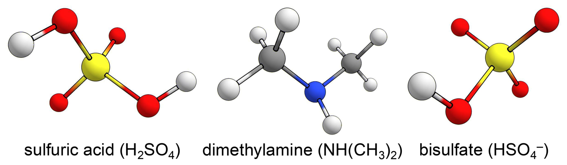
Figure 1 Ball-and-stick representations of sulfuric acid, dimethylamine, and bisulfate. This study considers collision systems of sulfuric acid paired with itself, dimethylamine, and bisulfate. Atom color code: sulfur (yellow), oxygen (red), nitrogen (blue), carbon (gray), and hydrogen (white).

2.2 Machine learning interatomic potentials

2.2.1 PaiNN

The polarizable atom interaction neural network (PaiNN) extends the message-passing formalism of the SchNet architecture by incorporating rotation-equivariant features to handle vectorial information (Schütt et al., 2021). This enables the representation of directional properties, which is essential for accurately describing forces, dipoles, and other tensorial quantities. PaiNN has been trained successfully on relatively small datasets, achieving accuracy competitive with kernel methods (Schütt et al., 2021).

The standard PaiNN architecture is not explicitly charge-aware and lacks long-range electrostatic or dispersion corrections. Instead, the model handles charged systems by implicitly learning the local, short-range effects of the charge directly from the energies and forces provided in the training data. However, a limitation of this purely local approach in the context of gas-phase collisions is that interactions cannot be transmitted between atoms separated by more than the cutoff distance without intermediate atoms to mediate the message passing. Increasing the cutoff can capture these long-range effects, but at the expense of higher computational cost and potentially reduced accuracy, as the model must learn to generalize over a significantly larger spatial domain.

2.2.2 AIMNet2

AIMNet2 is the second generation of the Atoms-In-Molecules Neural Network developed by Anstine et al. (2025). Using a message-passing architecture, the model iteratively refines invariant representations of local atomic environments, defined by radial symmetry functions, to build complex “atom-in-molecule” (AIM) embeddings. While directional dependencies are not enforced through explicit equivariance, AIMNet2 captures these effects implicitly through its atom-centered representations and iterative message passing. A key feature of AIMNet2 is its generalized embedding strategy, which avoids element-specific subnetworks and allows the model to flexibly represent highly diverse chemical compositions.

Beyond its local representations, AIMNet2 explicitly incorporates electronic and long-range physical effects. The architecture is charge-aware, using the total molecular charge as an input parameter to dynamically infer atom-centered partial charges during the message-passing phase. These partial charges are iteratively updated through a neural charge equilibration (NQE) scheme. The total potential energy is then calculated as the sum of the local configurational energy, explicit Coulombic electrostatic interactions derived from the learned partial charges, and a D3(BJ) dispersion correction (Grimme et al., 2010, 2011).

Designed for generalizability, AIMNet2 natively supports systems with different charge states and spin multiplicities. By explicitly accounting for these varying electronic states and long-range interactions, the model is well-suited for a wide range of chemically complex systems.

2.2.3 Delta-learning

Rather than training directly on molecular properties (e.g., electronic energies and forces) at a high level of theory, one can train on the difference between the high-level target and a more computationally efficient, lower-level method. In this framework, molecular dynamics (MD) simulations are performed at the lower level of theory but are corrected to approximate the high level of theory (Bogojeski et al., 2020). When the two levels of theory are correlated, this delta-learning approach can substantially reduce model errors (Ramakrishnan et al., 2015). The main drawback is that while the evaluation of the machine learning model is typically fast, the overall simulation speed is fundamentally limited by the computational cost of the lower-level baseline. In this work, we applied delta-learning using the PaiNN architecture to learn the correction between GFN1-xTB (Grimme et al., 2017) as the low-level baseline and ωB97X-3c (Müller et al., 2023) as the high-level method. We refer to this approach as Δ-PaiNN.

2.2.4 Data generation

For each of the three collision systems, we performed collision trajectory simulations at 300 K (output frequency of 100 steps) and umbrella sampling simulations at 300 and 500 K (output frequency of 250 steps) using the GFN1-xTB method (TBlite, version 0.2.1) (Ehlert, 2022), following the methodologies detailed in Sect. 2.3.2 and 2.3.3. All structures from a given system were pooled into a unified candidate dataset.

To construct a comprehensive training set, we employed a sampling strategy guided by the potential of mean force (PMF; see Sect. 2.3.3) along the center of mass distance between the collision partners. Candidate structures were binned by center-of-mass distance, and the number of samples selected per bin was determined by a weighted combination of the local PMF curvature and the raw sampling density. This ensures that regions where the potential energy surface (PES) changes rapidly along the collision coordinate are sampled more densely. Collision trajectory data were included to capture both non-interacting configurations and high-energy collision events, while the 500 K umbrella sampling data were incorporated to cover high-energy fluctuations and prevent model instability during thermal excursions.

Within each bin, we enforced structural diversity using a root-mean-square deviation (RMSD) filter. The RMSD threshold was dynamically relaxed near the PMF minimum to capture equilibrium fluctuations, while a stricter threshold was applied in high-energy regions to maximize configurational coverage. Finally, a global RMSD filter was applied to remove any remaining near-duplicates across the entire dataset, resulting in a final training set of 20 000 structures per system.

Atomic forces of the selected structures were obtained through potential energy gradient calculations with respect to the nuclear coordinates using GFN1-xTB (TBLite, version 0.2.1) and ωB97X-3c (ORCA, version 6.0.1) (Neese, 2012). Owing to the high computational cost, no direct MD simulations were run at the ωB97X-3c level. Instead, it was assumed that the GFN1-xTB PES sufficiently overlaps with the relevant regions of the ωB97X-3c PES. This assumption holds as long as the GFN1-xTB PES has the same topological features as the ωB97X-3c PES in the relevant regions. Small structural discrepancies are corrected, as the higher-level nuclear gradients provide a net force directing the geometry toward the true ωB97X-3c minimum. The assumption, however, breaks down if important regions of the ωB97X-3c PES are entirely missing from the GFN1-xTB PES. While this is unlikely for the relatively simple collision systems studied here, more complex clusters may require the dataset to be augmented with unvisited structures.

We note that while ωB97X-3c is used in this study, atomic forces can be calculated using any quantum chemistry method on the GFN1-xTB structures to obtain a training set at that level of theory.

2.3 Molecular dynamics simulations

2.3.1 Force calculations

In MD simulations, atomistic trajectories are generated by integrating Newton's equations of motion over discrete time steps. At each step, the forces acting on the nuclei are computed, and the system is propagated classically.

In this study, we employed several methods for force evaluation. Simulations using the semi-empirical GFN1-xTB method (Grimme et al., 2017) and the trained AIMNet2 and PaiNN models were performed within the Atomic Simulation Environment (ASE) (Hjorth Larsen et al., 2017). These calculations were executed through the tblite (Ehlert, 2022), aimnet2ase, and SchNetPack (Schütt et al., 2024) calculators, respectively. Furthermore, we employed a Δ-learning approach (Δ-PaiNN), wherein baseline GFN1-xTB forces were corrected by a model trained on the difference between GFN1-xTB and the target ωB97X-3c theory (or GFN1-xTB itself for validation).

Additionally, classical MD simulations were performed using the OPLS-AA force field (Jorgensen et al., 1996). These simulations were carried out with the LAMMPS (Large-scale Atomic/Molecular Massively Parallel Simulator) code (Plimpton, 1995; Thompson et al., 2022). A detailed description of the OPLS-AA parameters employed in this work can be found in Sect. S1 of the Supplement.

2.3.2 Collision trajectory simulations

Canonical collision rate coefficients are given by

$$\begin{array}{}\text{(1)}& \mathit{\beta }=\mathrm{2}\mathit{\pi }\underset{\mathrm{0}}{\overset{\mathrm{\infty }}{\int }}\mathrm{d}{v}_{\mathrm{0}}\underset{\mathrm{0}}{\overset{\mathrm{\infty }}{\int }}{v}_{\mathrm{0}}{f}_{\mathrm{MB}}\left(v_{\mathrm{0}}\right)b{P}_{\mathrm{c}}(v_{\mathrm{0}},b)\mathrm{d}b,\end{array}$$

where v₀ is the initial relative velocity between the collision partners, f_MB represents the Maxwell–Boltzmann relative speed distribution, and P_c(v₀,b) is the collision probability. The impact parameter b is defined as the perpendicular distance between the initial velocity vectors of the two partners.

To obtain collision rate coefficients from MD simulations, we approximated Eq. (1) with a Riemann sum. The initial relative velocity v₀ was sampled from 50 to 800 m s⁻¹ in steps of 50 m s⁻¹. This velocity range covers 99 % of the Maxwell–Boltzmann distribution for all systems. The impact parameter b ranged from 0 to 20 Å in steps of 1 Å for the neutral systems (H₂SO₄–H₂SO₄ and H₂SO₄–NH(CH₃)₂), and was extended to 60 Å for the ionic H₂SO₄–${\mathrm{HSO}}_{\mathrm{4}}^{-}$ system. While a maximum impact parameter of 20 Å was sufficient for the neutral pairs (Halonen et al., 2019; Neefjes et al., 2022), the larger cutoff for the ionic system was necessary because electrostatic attraction maintains non-negligible collision probabilities at much greater distances.

For each (v₀, b) pair, we performed 100 independent trajectory simulations. The collision probability P_c(v₀,b) is estimated as the fraction of trajectories that result in a collision. A collision is defined to occur if the center-of-mass distance between the partners falls below the sum of their hard-sphere radii, derived from their liquid bulk densities, for at least one output frame. These sums are 5.5, 5.7, and 5.5 Å for the H₂SO₄–H₂SO₄, H₂SO₄–NH(CH₃)₂, and H₂SO₄–${\mathrm{HSO}}_{\mathrm{4}}^{-}$ systems, respectively.

Prior to the collision simulations, the monomers were individually equilibrated in NVT simulations using the GFN1-xTB method (TBlite, version 0.2.1). Atomic velocities were initialized from a Maxwell–Boltzmann distribution at 300 K, and the temperature was maintained by a Langevin thermostat with a friction constant of 0.1 fs⁻¹. Each equilibration run lasted 13 ns with a 1 fs timestep and an output frequency of 1000 steps. Convergence of the total, translational, vibrational, and rotational temperatures was achieved after approximately 3 ns. The remaining 10 ns were sampled every 1000 steps to yield 10 000 equilibrated starting configurations.

At the start of each collision trajectory, two monomers were randomly selected from their respective equilibrated structures and placed 30 Å apart along the x axis. This value was chosen as a compromise between minimizing initial interaction forces and limiting computational cost. The collision partners were offset along the z axis by the impact parameter b and assigned opposing velocities of v_x = $\pm v_{\mathrm{0}}/\mathrm{2}$. Each trajectory was propagated in the NVE ensemble for a duration sufficient for a non-interacting particle to traverse the initial separation plus the offset b, with an additional safety margin of 10 Å.

2.3.3 Umbrella sampling

We performed umbrella sampling simulations along the center-of-mass distance coordinate r between the collision partners (Torrie and Valleau, 1977). The reaction coordinate was discretized into 91 windows centered from 2.0 to 20.0 Å with a step size of 0.2 Å. In each window, the system was restrained by a harmonic bias potential V_bias = $\frac{\mathrm{1}}{\mathrm{2}}{k}_{\mathrm{bias}}(r-r_i{)}^{\mathrm{2}}$, where r_i is the window center and k_bias = 100 kcal mol⁻¹ Å⁻², consistent with the parameters used by Kubečka et al. (2025).

Starting configurations were drawn from the final 10 000 output frames of the equilibration trajectories described in Sect. 2.3.2. These structures were translated to align with the center of the target umbrella window. For windows at short distances (r < 6.0 Å), where direct placement might result in steric clashes, the collision partners were initially placed 6.0 Å apart. The bias potential was then gradually increased from 0 to 100 kcal mol⁻¹ Å⁻² over the first 2000 time steps.

To enhance sampling, ten independent simulations were performed for each window. Each simulation began with 100 000 steps of equilibration in the NVT ensemble (Langevin thermostat, friction 0.1 fs⁻¹), followed by a 500 000-step production run using the canonical sampling through velocity rescaling (CSVR) thermostat with a time constant of 25 fs (Bussi et al., 2007). The output frequency for both thermodynamic data and structural configurations was set to 250 steps.

The unbiased free energy profile was reconstructed using the umbrella integration method as implemented in the umbrella_integration code (Stroet and Deplazes, 2016). Because this profile represents the Helmholtz free energy A(r) of finding particles at a distance r in three-dimensional space, it includes an entropic term due to the increasing volume of the spherical shell 4πr²dr. To obtain the effective interaction potential w(r) (the one-dimensional PMF), we subtracted this radial entropic contribution:

$$\begin{array}{}\text{(2)}& w\left(r\right)=A\left(r\right)-\left[-k_{\mathrm{B}}T\ln \left(\mathrm{4}\mathit{\pi }{r}^{\mathrm{2}}\right)\right],\end{array}$$

where k_B is the Boltzmann constant and T the temperature.

3 Results and discussion

3.1 Hyperparameter tuning

Training efficiency and model performance are dependent on the choice of hyperparameters. To optimize the PaiNN and AIMNet2 architectures for our systems, we performed hyperparameter tuning using the Weights and Biases (W&B) platform (Biewald, 2020). For PaiNN, we tuned the number of features, batch size, number of blocks, and radial basis size. For AIMNet2, we tuned the AIM size, number of features, batch size, batches per epoch, vector channels, radial basis size, and learning rate. Testing three values for each hyperparameter results in a total of 81 combinations for PaiNN and 729 for AIMNet2, making a systematic hyperparameter grid search computationally prohibitive. Consequently, we employed a random search.

100-epoch long tuning runs were performed on a subset of 2000 structures labeled at the GFN1-xTB level of theory. The target was to minimize the validation loss, defined as a weighted sum of the mean squared errors (MSE) in potential energies, atomic force components, and, in the case of AIMNet2, atomic partial charges. Given the importance of accurate forces for stable molecular dynamics (MD) simulations, and the fact that force data (3×N_atom) vastly outnumber energy data, we assigned a greater weight to the force loss. For PaiNN, the energy:force_components weight ratio was set to 1 : 99. For AIMNet2, which also predicts partial charges, the energy:force_components:atomic_charges weights were set to $\mathrm{9}:\mathrm{90}:\mathrm{1}$.

We completed 70 unique tuning runs for PaiNN and 50 for AIMNet2. The results are visualized in the Supplement (Figs. S1 and S2). Tables 1 and 2 summarize the tested values and quantify the impact of each hyperparameter using W&B's hyperparameter importance and Pearson correlation metrics. The importance metric, derived from a random forest algorithm, quantifies the relative impact of each hyperparameter on the validation loss. A negative correlation indicates that increasing the parameter value reduces the validation loss.

Table 1 Tested hyperparameter values for PaiNN, including the hyperparameter importance and Pearson correlation with respect to the validation loss obtained from Weights and Biases (Biewald, 2020).

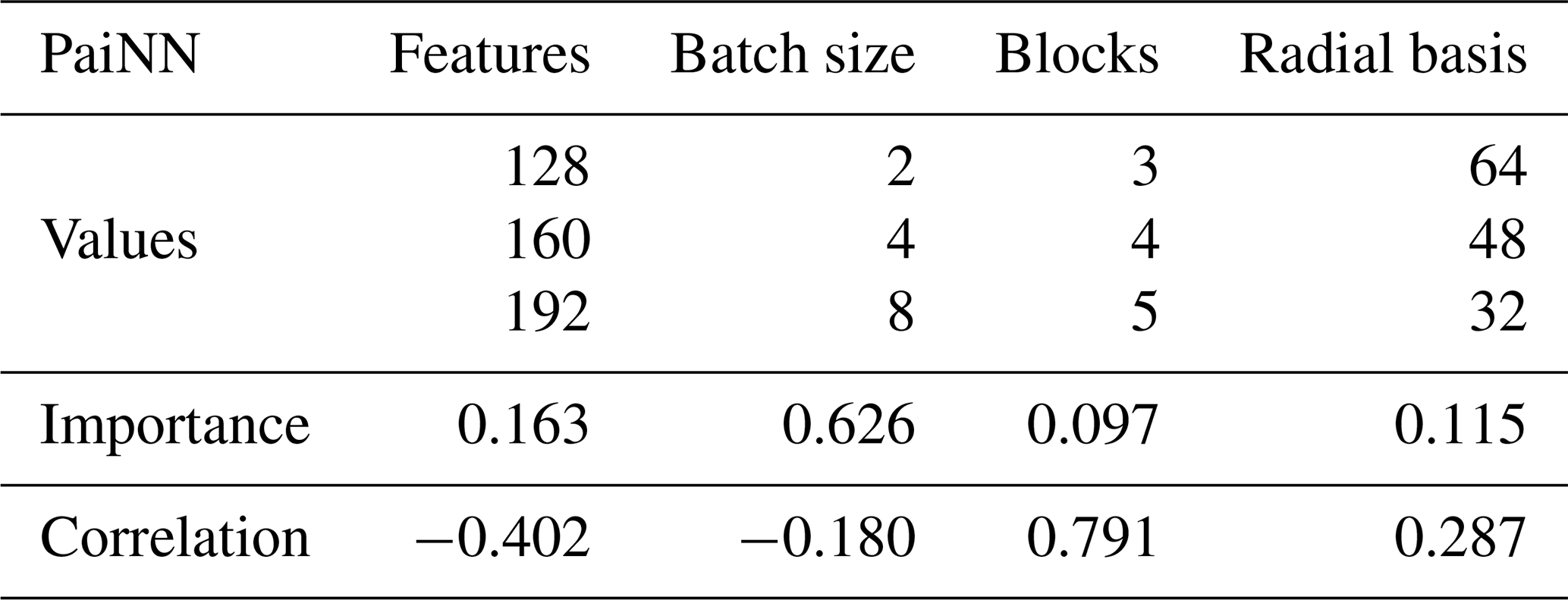
Table 2 Tested hyperparameter values for AIMNet2, including the hyperparameter importance and Pearson correlation with respect to the validation loss obtained from Weights and Biases (Biewald, 2020).

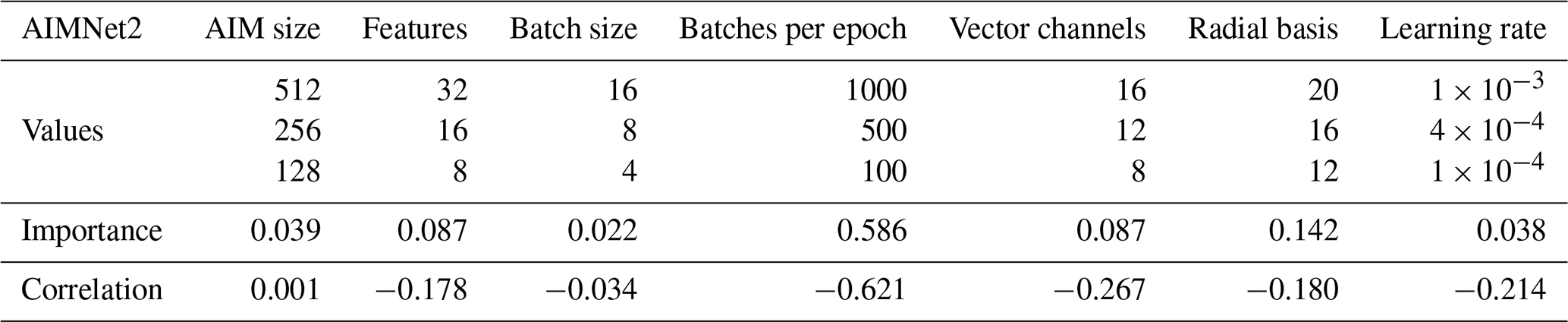
For PaiNN, the batch size and number of features were identified as the most important hyperparameters, with a smaller batch size and a higher number of features correlating with improved performance. In contrast, for AIMNet2, the “batches per epoch” was the dominant hyperparameter. This difference stems from how each training framework defines an epoch. In PaiNN, an epoch follows the standard definition of a single, full pass through the training data. Thus, the training set size and batch size strictly determine the batches per epoch. However, the AIMNet2 framework decouples the definition of an epoch from the dataset size, operationally defining it as a user-specified number of steps before each validation check. Therefore, in AIMNet2, the product of the batch size and the batches per epoch determines the total number of samples processed per operational epoch. When this product is smaller than the training set size, a validation step is triggered before the model has seen all training samples. When the product exceeds the dataset size (e.g., using 1000 batches of size 16 means the AIMNet2 model processes 16 000 samples per validation cycle for our 2000-molecule dataset), the model sees data multiple times per epoch, which further aids convergence.

Based on these results, we selected the following hyperparameters for the final production models. For PaiNN (and Δ-PaiNN), we used 256 features, a batch size of 2, 4 interaction blocks, and a radial basis size of 32. For AIMNet2, we selected an AIM size of 128, 16 features, a batch size of 8, 16 vector channels, a radial basis size of 20, and a learning rate of 4 × 10⁻³. To account for the larger production dataset, the number of batches per epoch was increased to 4000. The short-range cutoff for AIMNet2 was set to 5 Å. Since PaiNN lacks explicit long-range interactions beyond the local environment, its cutoff was extended to 10 Å. A full list of hyperparameters for each model is provided in Sect. S3.

It is important to note that we did not necessarily identify the optimal hyperparameter combination for our systems. For instance, while our 100-epoch tuning procedure offers a reasonable indication of training behavior, some hyperparameters might converge slower but dominate during longer training. Identifying the best training settings would require a systematic search over a broader range of values. While automated techniques such as Bayesian optimization (Stuke et al., 2021) could be explored for more complex systems in future work, the chosen hyperparameters provide sufficiently low test errors for the collision systems studied here, as discussed in the following subsection.

3.2 Training

Using the hyperparameters determined in Sect. 3.1, we trained AIMNet2, PaiNN, and Δ-PaiNN models for each system using either GFN1-xTB or ωB97X-3c reference data (20 000 structures per system). Training durations were set to 1000 (AIMNet2), 600 (PaiNN), and 400 (Δ-PaiNN) epochs, chosen to balance their respective convergence rates with computational cost. Model performance was evaluated on an independent test set of ∼ 2000 structures per system, sampled from the 300 K umbrella sampling trajectories across both center-of-mass distance (between 2.0 and 20.0 Å) and potential energy. We report the mean absolute errors (MAEs) for electronic energies (E_el) and component-wise forces (F) in Table 3. As a sanity check, we also trained a Δ-PaiNN model using GFN1-xTB as both the baseline and the target reference for the H₂SO₄–H₂SO₄ system. Since this model was trained on the difference between two identical levels of theory, it should essentially predict zero correction.

Table 3 Mean absolute errors (MAE) of the machine learning models relative to the level of theory they were trained on for electronic energies (E_el) and component-wise forces (F) across the three studied systems: H₂SO₄–H₂SO₄, H₂SO₄–NH(CH₃)₂, and H₂SO₄–${\mathrm{HSO}}_{\mathrm{4}}^{-}$. Results are reported for AIMNet2, PaiNN, and Δ-PaiNN trained on GFN1-xTB and ωB97X-3c training data. Units: E_el in kcal mol⁻¹ and F in kcal mol⁻¹ Å⁻¹.

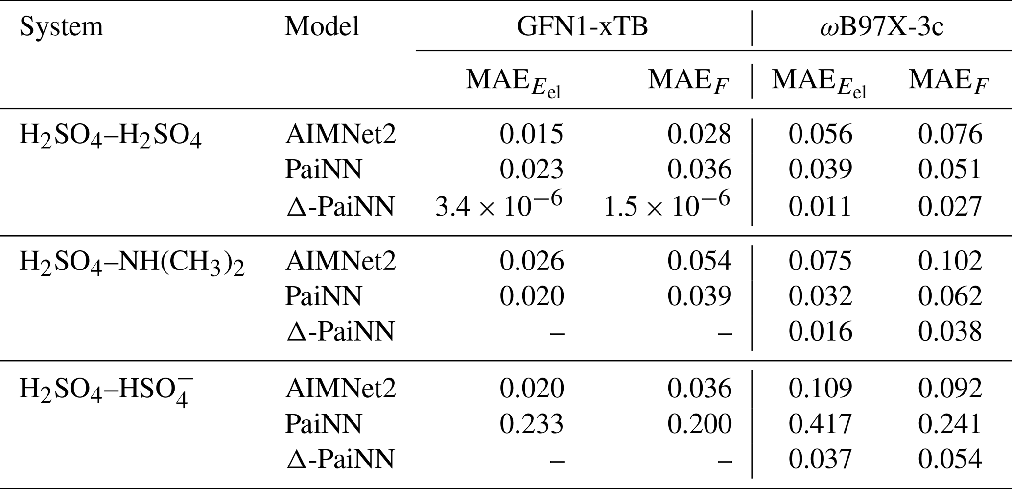
In general, the models achieve excellent accuracy. All MAEs fall below the standard chemical accuracy thresholds of 1 kcal mol⁻¹ for energies and 1 kcal mol⁻¹ Å⁻¹ for forces. Notably, for the neutral H₂SO₄–H₂SO₄ and H₂SO₄–NH(CH₃)₂ systems, the reproduction errors are exceptionally low, with MAEs below 0.1 kcal mol⁻¹ and 0.1 kcal mol⁻¹ Å⁻¹. The Δ-PaiNN methodology proves particularly effective. It correctly predicts negligible corrections in the GFN1-xTB sanity check, and consistently achieves the lowest errors when ωB97X-3c is the target level. The highest energy error was observed for the H₂SO₄–${\mathrm{HSO}}_{\mathrm{4}}^{-}$ system trained with PaiNN on ωB97X-3c, as expected due to the lack of long-range interactions.

To better understand the distribution of these errors, we analyzed the energy deviations as a function of center-of-mass distance (Fig. 2) for the ωB97X-3c target level of theory. For the H₂SO₄-H₂SO₄ system, the errors are consistently low across the entire coordinate. By contrast, the H₂SO₄–NH(CH₃)₂ system exhibited larger errors at short distances (r < 3 Å). These deviations correspond to the highly repulsive regime of the potential energy surface (PES), where steric hindrance drives the potential energy tens of kcal mol⁻¹ above the minimum. Consequently, the probability of visiting these configurations during standard MD is negligible.

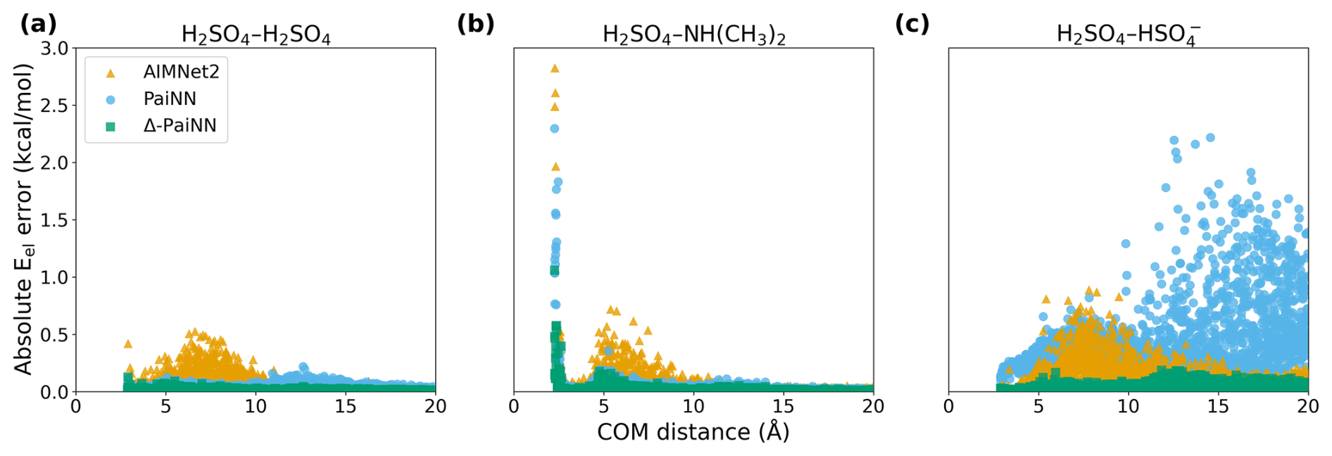
Figure 2 Electronic energy reproduction errors for machine learning models trained on ωB97X-3c data relative to the ωB97X-3c level of theory, shown as a function of the center-of-mass (COM) distance across the three studied systems: H₂SO₄–H₂SO₄ (a), H₂SO₄–NH(CH₃)₂ (b), and H₂SO₄–${\mathrm{HSO}}_{\mathrm{4}}^{-}$ (c). Results are shown for AIMNet2, PaiNN, and Δ-PaiNN.

In contrast, the ionic H₂SO₄–${\mathrm{HSO}}_{\mathrm{4}}^{-}$ system illustrates the inherent limitations of applying a purely local representation to systems with strong long-range interactions. Although the electronic energy MAE for PaiNN appears relatively low, the distance-resolved error plot (Fig. 2c) reveals significant deviations at separations r > 10 Å. At these large distances, the training data already capture substantial stabilization energy due to long-range ion–dipole interactions, which also induce slight geometric distortions in the approaching collision partners. However, because PaiNN employs a strict 10 Å spatial cutoff, it evaluates the system as two completely isolated, non-interacting collision partners. During training, the model must map the significantly lowered potential energy of the interacting system to these isolated, slightly distorted molecular structures. Consequently, PaiNN erroneously learns to associate the long-range electrostatic stabilization entirely with these slight internal structural changes. In essence, the model is forced to view this distorted geometry as the lowest energy conformer of the isolated molecule, creating an artificial global minimum that fundamentally distorts the PES.

3.3 Potentials of mean force

3.3.1 GFN1-xTB training data

The potential of mean force (PMF) along the center-of-mass distance represents the effective free energy averaged over all collision orientations accessed during the simulations, showing how the system's stability changes as the collision partners approach (see e.g., Fig. 3). The well depth and shape provide information on the binding strength, while the shoulder towards larger distances reflects the strength of long-range interactions.

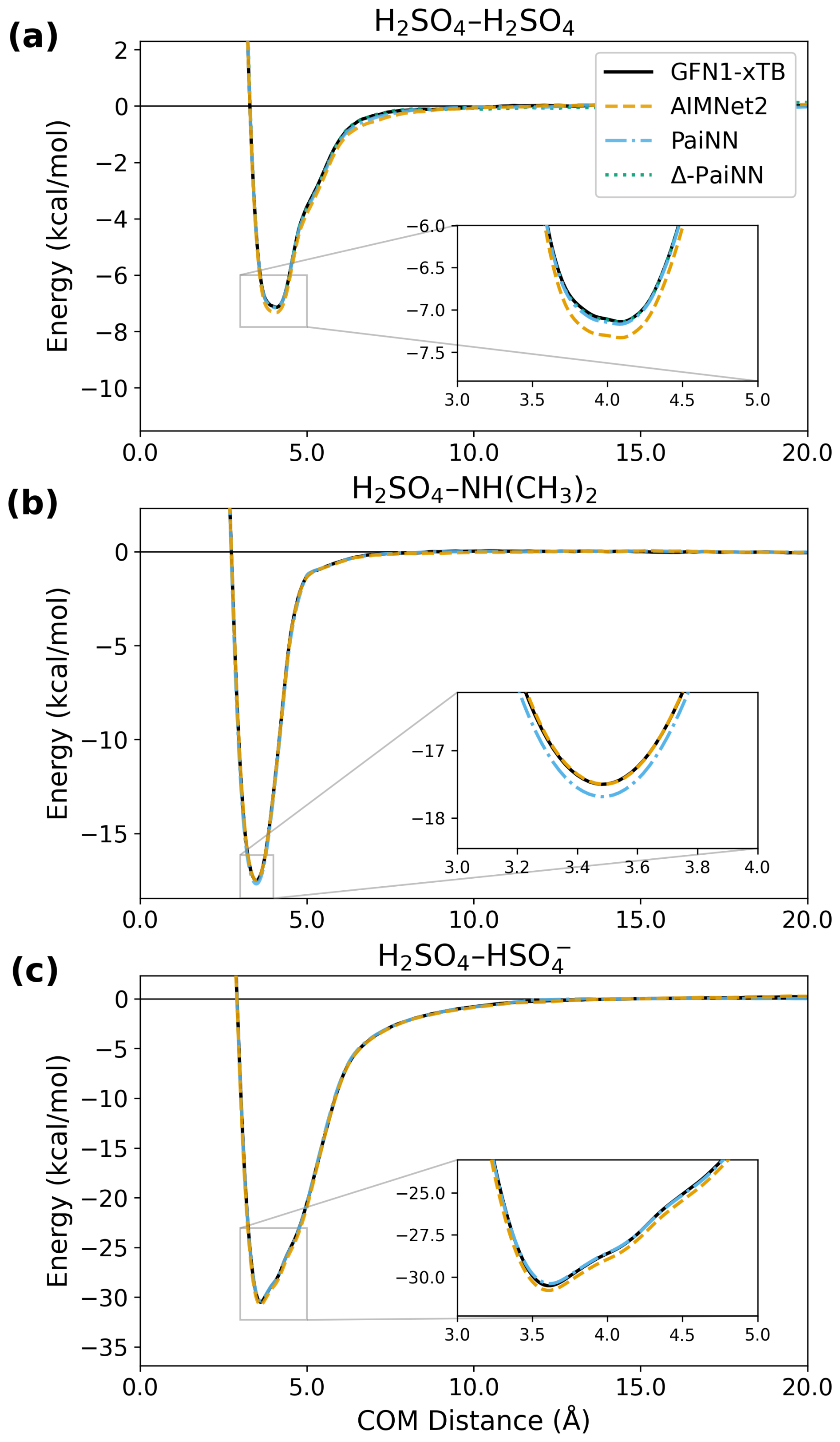
Figure 3 Potentials of mean force (PMF) as a function of center-of-mass (COM) distance for the H₂SO₄–H₂SO₄, H₂SO₄–NH(CH₃)₂, and H₂SO₄–${\mathrm{HSO}}_{\mathrm{4}}^{-}$ systems. The profiles compare the reference GFN1-xTB level of theory with predictions from AIMNet2, PaiNN, and Δ-PaiNN models trained on GFN1-xTB data.

Although all the models achieved low mean absolute errors and included high-energy structures (from simulations at 500 K) in the training sets, the umbrella sampling simulations occasionally explored untrained regions of the PES. This caused a breakdown in dynamics and resulted in unphysical geometries. Including these trajectories introduced large errors into the predicted PMFs. Consequently, we implemented a script to filter these simulations by monitoring the distance between any two hydrogen atoms. We discarded any simulation where the maximum distance exceeded the window center by more than 8.0 Å or the minimum distance fell below 1.0 Å. While this script does not test for every possible failure, it is a reasonable compromise between filtering out erroneous simulations and efficiently automating the process over the large amount of data generated. Approximately half of the umbrella sampling calculations contained failed simulations. However, no more than three independent simulation runs were ever removed from a single window. This ensured that every window retained at least 7 simulations (500 000 steps each, saved every 250 steps), providing a dataset of at least 14 000 structures per window for constructing the PMF. A detailed list of removed simulations is provided in Sect. S4.

Figure 3 shows the PMFs for all three systems calculated using AIMNet2 and PaiNN (trained on GFN1-xTB), compared against the GFN1-xTB reference. For the H₂SO₄–H₂SO₄ system, the Δ-PaiNN model trained on GFN1-xTB was again included as a sanity check. While this model should theoretically reproduce the GFN1-xTB reference PMF, small deviations are nonetheless expected due to the inherent uncertainty associated with finite umbrella sampling. Additionally, because the machine learning models lack training data in the highly repulsive, physically inaccessible regimes at short distances, much larger deviations can occur in these regions (see Fig. S3).

Table 4 lists the root-mean-square errors (RMSEs) of the predicted PMFs relative to the reference. We report the RMSE only between the point where the PMF drops below zero in the short-range repulsive region and the first point it returns to zero in the long-range non-interacting region. At shorter distances, the steep energies of the repulsive wall lead to sparse training data coverage, which can result in localized high errors. However, because these configurations are physically inaccessible at atmospheric temperatures, excluding this region ensures the reported RMSE reflects the model's performance in the region relevant to the clustering dynamics. Conversely, we exclude the asymptotic long-range tail because the collision partners are essentially non-interacting here. Including an extensive non-interacting region, which is well-sampled and exhibits minimal energy variation, would disproportionately lower the average error, masking the model's performance in the interaction region. While the PMF should theoretically approach zero asymptotically, sampling noise causes the long-range zero-crossing to occur at finite distances (< 20 Å) for the systems studied here.

Table 4 Root-mean-square errors (RMSE) in kcal mol⁻¹ for the potentials of mean force (PMFs) predicted by the machine learning models relative to the GFN1-xTB reference. The RMSE is evaluated between the point where the PMF drops below zero in the short-range repulsive region and the first point it returns to zero in the long-range non-interacting region.

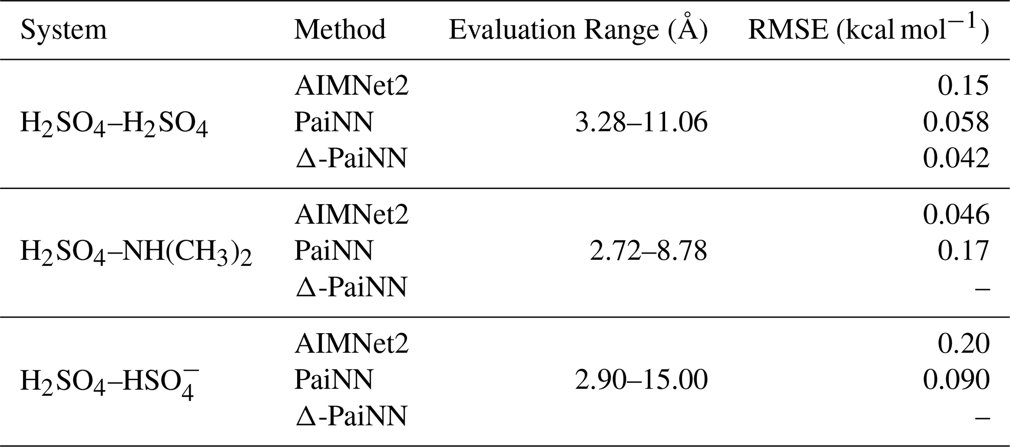
All models exhibit excellent agreement with the reference PMF. The highest observed RMSE is 0.20 kcal mol⁻¹ for AIMNet2 applied to the H₂SO₄–${\mathrm{HSO}}_{\mathrm{4}}^{-}$ system, which is five times lower than the standard threshold for chemical accuracy (1 kcal mol⁻¹). In other words, the reproduction error introduced by the machine learning models is negligible compared to generally accepted error margins in computational chemistry. PaiNN performs better than AIMNet2 for the H₂SO₄–H₂SO₄ and H₂SO₄–${\mathrm{HSO}}_{\mathrm{4}}^{-}$ systems, while the opposite is true for the H₂SO₄–NH(CH₃)₂ system. Across the three systems, the average error is 0.13 kcal mol⁻¹ for AIMNet2 and 0.11 kcal mol⁻¹ for PaiNN. Thus, PaiNN performs slightly better overall, though the difference is marginal.

The performance of PaiNN on the H₂SO₄–${\mathrm{HSO}}_{\mathrm{4}}^{-}$ system is somewhat surprising, given that it cannot capture interactions beyond its 10 Å local atomic environment cutoff. However, Fig. 3 shows that the PMF effectively decays to zero around 13 Å. As long as any two atoms between the collision partners remain within 10 Å, the message-passing algorithm treats the system as connected. Given that the sum of the hard-sphere radii for H₂SO₄–${\mathrm{HSO}}_{\mathrm{4}}^{-}$ is approximately 3.89 Å (Neefjes et al., 2022), PaiNN with cutoff 10 Å can model interactions up to at least 13 Å center-of-mass distance. We note, however, that while the PMF vanishes at 13 Å, this represents an average energy. Individual trajectories with specific orientations may still exhibit longer-range interactions.

3.3.2 ωB97X-3c training data

We subsequently trained AIMNet2, PaiNN, and Δ-PaiNN on the higher-level ωB97X-3c data to generate the PMFs presented in Fig. 4. The PMFs obtained with the GFN1-xTB method are shown for comparison. First, we observe that all three ML models are in excellent agreement with each other. While obtaining a reference PMF directly using the ωB97X-3c method is computationally prohibitive, the fact that these models, utilizing distinct algorithms, predict very similar PMFs strongly suggests that the ωB97X-3c potential energy surface is accurately reproduced.

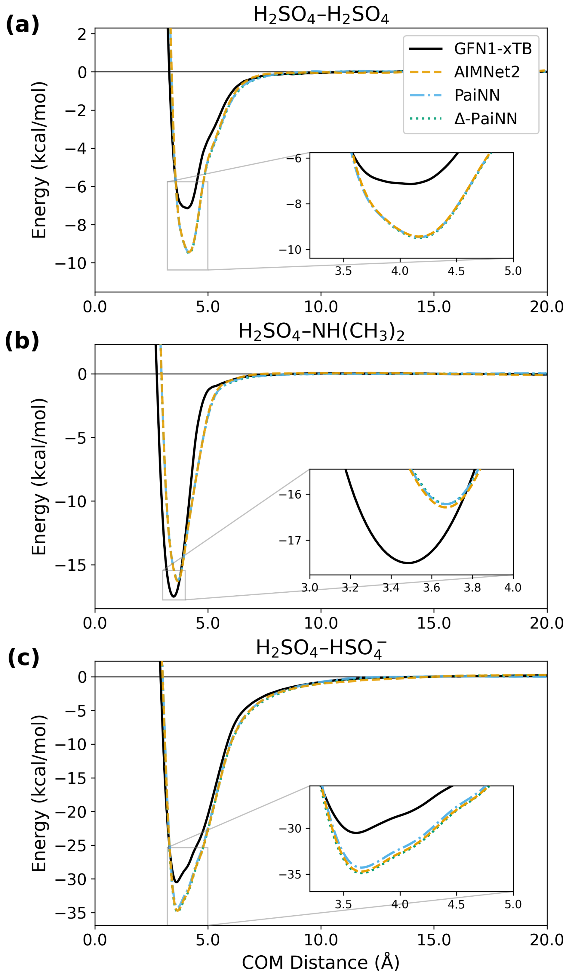
Figure 4 Potentials of mean force (PMF) as a function of center-of-mass (COM) distance for the H₂SO₄–H₂SO₄, H₂SO₄–NH(CH₃)₂, and H₂SO₄–${\mathrm{HSO}}_{\mathrm{4}}^{-}$ systems. The profiles compare the reference GFN1-xTB level of theory with predictions from AIMNet2, PaiNN, and Δ-PaiNN models trained on ωB97X-3c data.

Comparing the PMFs based on ωB97X-3c data to the GFN1-xTB reference, we observe that the shoulder regions are similar between methods, while the minima show significant differences. Most notably, ωB97X-3c predicts significantly different well depths: the minima for the H₂SO₄–H₂SO₄ and H₂SO₄–${\mathrm{HSO}}_{\mathrm{4}}^{-}$ systems are lower by 2.3 and 3.8 kcal mol⁻¹, respectively, compared to GFN1-xTB. For the H₂SO₄–NH(CH₃)₂ complex, the methods differ on both the position (shifted by 0.18 Å) and the depth (difference of 1.3 kcal mol⁻¹) of the minimum, indicating distinct lowest free energy geometries.

In several of our recent studies, we have integrated the PMF well to obtain binding free energy estimates (Kubečka et al., 2025; Neefjes et al., 2026). While GFN1-xTB can capture correct qualitative trends, obtaining quantitatively accurate binding energies requires higher levels of theory. Due to the computational cost of running MD with these methods, ML approaches must be employed.

3.4 Computational cost

We briefly discuss the training and evaluation of the computational costs for the three models. On an NVIDIA V100-16GB GPU, the AIMNet2, PaiNN, and Δ-PaiNN models, trained on 20,000 H₂SO₄–H₂SO₄ structures, complete approximately 30, 6, and 6 epochs per GPU hour, respectively. For evaluation, we performed umbrella sampling for the H₂SO₄–H₂SO₄ system (at the 4.0 Å window) on an Intel Xeon Gold 6248R CPU. Under these conditions, AIMNet2, PaiNN, and Δ-PaiNN achieved speeds of approximately 120 000, 130 000, and 65 000 steps per CPU hour, respectively. The performance of Δ-PaiNN is inherently limited by the computational cost of the baseline method (here GFN1-xTB), as both the baseline energy and the ML correction must be evaluated at every step. We note that these timings are highly dependent on the specific system architecture and software implementation. Specifically, our group has more extensive experience optimizing PaiNN compared to AIMNet2. Consequently, our PaiNN implementation may be more streamlined. Therefore, these timings should be considered indicative rather than a rigorous benchmark.

3.5 Collision probabilities

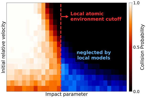
Collision rate coefficients are calculated via Eq. (1), where the collision probability P_c(v₀,b) is obtained from MD collision trajectory simulations over a relevant range of initial relative velocities v₀ and impact parameters b. Figure 5 compares the collision probabilities obtained from GFN1-xTB MD simulations with those from the AIMNet2 and PaiNN models trained on GFN1-xTB data. The AIMNet2 results are in excellent agreement with the GFN1-xTB reference, showing only a slightly lower collision probability in the tail towards higher b. Conversely, the PaiNN heat map clearly highlights the limitations of the local environment approximation for modeling collisions. Above the cutoff plus the sum of molecular radii (∼ 13.89 Å), the message-passing algorithm no longer detects interactions between the collision partners. Consequently, zero collisions are registered past 14 Å. We also note that even below 14 Å, PaiNN appears to underestimate the collision probability compared to the reference. Therefore, for systems with strong long-range interactions, it is necessary to employ a model that accounts for interactions beyond the local atomic environment cutoff, such as AIMNet2.

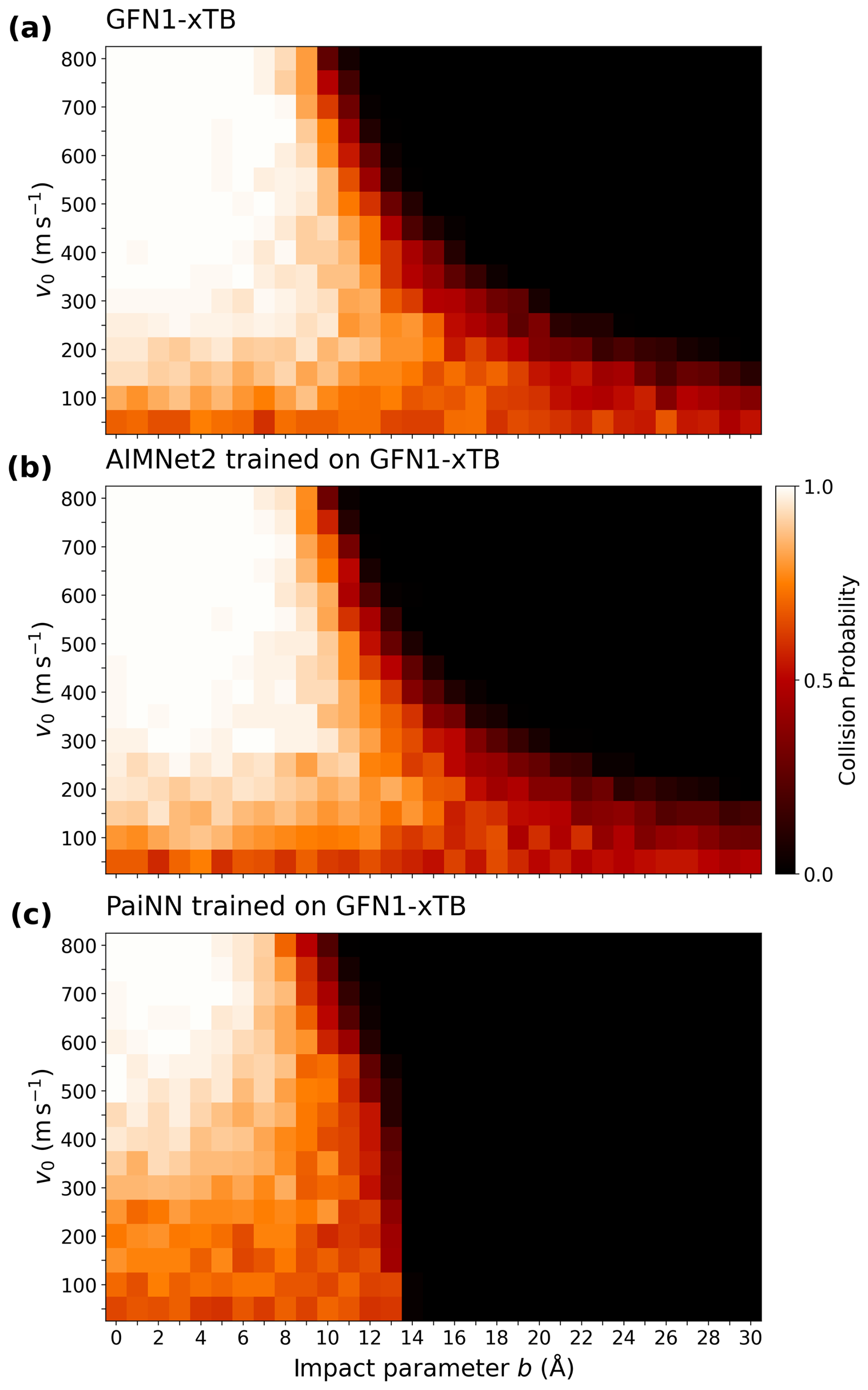
Figure 5 Comparison of collision probabilities derived from molecular dynamics simulations for the H₂SO₄–${\mathrm{HSO}}_{\mathrm{4}}^{-}$ system at 300 K. The heat maps show the probability distribution across impact parameter b and initial relative velocity v₀ for the reference GFN1-xTB method (a) and the AIMNet2 (b) and PaiNN (c) models trained on GFN1-xTB data.

The H₂SO₄–H₂SO₄ and H₂SO₄–NH(CH₃)₂ systems exhibit similar trends, although the discrepancies are less pronounced due to the weaker long-range interactions in these systems. These results are presented in Sect. S6.

3.6 Collision rate coefficients

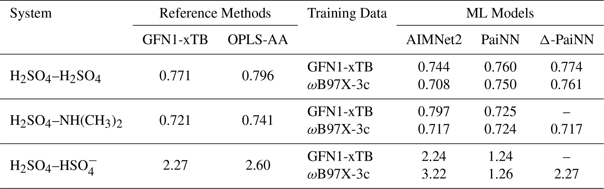
Using the collision probabilities, we calculated the corresponding canonical collision rate coefficients via Eq. (1). Table 5 presents these values, comparing the performance of the three ML models against the GFN1-xTB reference and the classical OPLS-AA force field.

Table 5 Collision rate coefficients calculated at 300 K using AIMNet2, PaiNN, and Δ-PaiNN compared to GFN1-xTB and OPLS-AA reference values. All values are in10⁻¹⁵ m³ s⁻¹.

We note that while pressure-independent canonical collision rate coefficients, as obtained here, are commonly employed in cluster distribution dynamics models, this relies on the assumption that the system is strongly bound and has enough degrees of freedom to effectively distribute excess collisional energy (Elm et al., 2020). This assumption is likely valid for larger clusters, given that the number of degrees of freedom strictly increases with cluster size, and binding energies generally do as well. However, dimers with fewer degrees of freedom that are less strongly bound, such as the H₂SO₄–H₂SO₄ system, might not effectively thermalize immediately after collision. Consequently, for these collisions, the true collision rate coefficient could be smaller than the coefficient calculated here, due to pressure dependence.

To contextualize the obtained collision rate coefficients, it is important to note that the accuracy of particle formation rates in cluster distribution dynamics simulations depends on both the collision and evaporation rate coefficients. Because evaporation rates depend exponentially on binding free energies, uncertainties in binding free energies typically outweigh errors in collision rate coefficients. An error of just 1 kcal mol⁻¹ in binding free energies introduces a factor of ∼ 5 uncertainty in the evaporation rate. As such, we consider an error of a factor of 1.5 in the collision rate coefficients acceptable. In the worst-case scenario where collision and evaporation rate coefficient errors compound in the same direction, a factor of 1.5 collision rate coefficient error would still result in an overall uncertainty in the particle formation rates of less than an order of magnitude.

Evaluated against this threshold, PaiNN yields notably lower rate coefficients for the charged H₂SO₄–${\mathrm{HSO}}_{\mathrm{4}}^{-}$ system. For both GFN1-xTB and ωB97X-3c training data, the model underestimates the rates by nearly 50 % (roughly a factor of 2) relative to the GFN1-xTB reference. As discussed in Sect. 3.5, this substantial deviation stems from the model's inability to detect collisions beyond its 10 Å cutoff, effectively neglecting the significant contribution of the long-range tail.

Conversely, for the neutral systems (H₂SO₄–H₂SO₄ and H₂SO₄–NH(CH₃)₂), the ML models trained on GFN1-xTB data exhibit excellent agreement with the reference calculations. All three architectures reproduce the GFN1-xTB reference rate coefficients closely, with the largest deviation observed for AIMNet2 applied to the H₂SO₄–NH(CH₃)₂ system (∼ 10 % discrepancy).

When targeting the higher-level ωB97X-3c theory, the predicted collision rate coefficients are generally similar to the GFN1-xTB reference values. The notable exception is the H₂SO₄–${\mathrm{HSO}}_{\mathrm{4}}^{-}$ system modeled with AIMNet2, where the predicted rate is significantly higher. An analysis of the collision probabilities (Figs. S6c and S4c) shows that this difference results primarily from increased collisions at low initial relative velocities. In the GFN1-xTB reference, collision probabilities in this region are low even at small impact parameters. This behavior has previously been attributed to repulsive electrostatic interactions as the collision partners approach (Halonen et al., 2019). However, AIMNet2 trained on the higher-level ωB97X-3c data does not exhibit this repulsion. This suggests that the repulsive feature observed in GFN1-xTB could be an artifact of the semi-empirical method failing to accurately describe the long-range potential.

The classical OPLS-AA force field also produces collision rates close to the GFN1-xTB reference values. For the charged H₂SO₄–${\mathrm{HSO}}_{\mathrm{4}}^{-}$ system, the OPLS-AA result lies between the GFN1-xTB reference and the AIMNet2 prediction trained on ωB97X-3c. Given that OPLS-AA relies on fixed partial charges, this agreement suggests that explicit dynamic electron density reorganization is not strictly necessary to model the collision process, provided the underlying electrostatic potential is sufficiently accurate. Simple fixed partial charges appear sufficient to model the approach, a finding consistent with observations by Knattrup et al. (2025).

Despite this accuracy in capturing collisions, classical force fields are insufficient for modeling the full nucleation process, as short-range interactions, particularly proton transfers, require an explicit quantum mechanical treatment. Proton transfers stabilize acid–base clusters (e.g., between sulfuric acid and amines) which play a crucial role in atmospheric particle formation. Classical force fields like OPLS-AA are fundamentally unable to model these proton transfer events. Figure 6 illustrates the geometry of the H₂SO₄–NH(CH₃)₂ system immediately before a collision and after cluster formation. A proton initially bound to H₂SO₄ transfers to NH(CH₃)₂ during the clustering process, eventually becoming separated by more than 5 Å from its original oxygen atom. Simulating this separation is impossible with classical harmonic bond potentials. In contrast, both the GFN1-xTB method and all three tested ML models successfully capture these dynamic proton transfers.

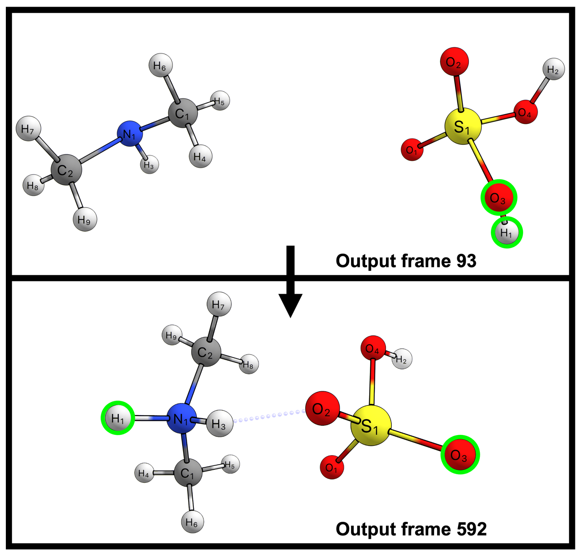
Figure 6 Stick-and-ball representations of two frames from a molecular dynamics collision trajectory simulation of the sulfuric acid–dimethylamine system. Frame 93 shows the system just before collision, with hydrogen H₁ bonded to oxygen O₃ of sulfuric acid (highlighted with green circles). Output frame 592 shows a post-collision configuration, where hydrogen H₁ is now bonded to nitrogen N₁ of dimethylamine, while oxygen O₃ of sulfuric acid is more than 5 Å away. Atom color code: sulfur (yellow), oxygen (red), nitrogen (blue), carbon (gray), and hydrogen (white).

4 Conclusions

With recent advances in machine learning interatomic potentials, molecular dynamics has rapidly evolved into a field capable of directly modeling cluster formation for large systems over long timescales, all while reproducing the accuracy of high-level quantum chemistry theory. While the low concentrations of cluster-forming vapors in the atmosphere still necessitate approximations (such as artificially increased concentrations), the ability to model the inherently dynamic cluster formation process at this level of theory is a significant breakthrough. However, machine learning models are frequently treated as black boxes. It is crucial that the increased accuracy in modeling complex short-range interactions, such as cluster reconfiguration and proton transfer, does not come at the expense of the long-range interactions that govern the initial collisions.

To address this, we evaluated the AIMNet2 and PaiNN machine learning methodologies, as well as a Δ-PaiNN method (using PaiNN to learn the correlation between GFN1-xTB and high-level quantum theory), for their ability to reproduce collision dynamics for sulfuric acid with either sulfuric acid, dimethylamine, and bisulfate. All models achieved low mean absolute errors on test sets and showed excellent agreement with GFN1-xTB reference potentials of mean force.

However, when comparing collision rate coefficients, we observe significant differences. For the charged sulfuric acid–bisulfate system, PaiNN predicted collision rate coefficients approximately 50 % lower than the reference method. This error arises from the strictly short-ranged nature of the local atomic environment approximation. PaiNN only considers interactions up to a specific cutoff (here, 10 Å). In charged systems, strong long-range interactions can induce collisions from distances far beyond this cutoff. AIMNet2 avoids this issue by augmenting its local short-ranged modeling with explicit long-range Coulombic interactions (via learned partial charges) and dispersion corrections, allowing it to accurately replicate the reference rates.

Our intention is not to highlight a specific failing of PaiNN, but rather to use it as a case study. We demonstrate that low mean absolute errors on a static test set do not automatically guarantee that a model is fit for purpose in dynamic simulations. A model must always be validated against reference data for the specific physical properties of interest. We also note that while we used a generous 10 Å cutoff, many standard implementations use 5 Å. At such small cutoffs, similar discrepancies would likely appear even for neutral systems. That being said, we note that the PaiNN architecture could be adapted to also include explicit long-range interactions, similar to AIMNet2.

In conclusion, we urge researchers to validate trained machine learning models beyond simple scalar metrics like mean absolute errors and root mean square errors, as these condensed measures can mask specific physical limitations. In future work, we will employ AIMNet2 and PaiNN, applying each where it is most appropriate, to directly study the cluster formation of nucleation precursor vapors with accurate descriptions of both short- and long-range interactions.