Updated global and regional trends of stratospheric ozone profiles

We present updated evaluation of stratospheric ozone profile trends in the 60° S–60° N latitude range using long-term ground-based and satellite climate data records, as well as simulations by chemistry-climate models. The trends are evaluated using the LOTUS (Long-term Ozone Trends and Uncertainties in the Stratosphere) regression model.

Analyses of satellite data confirm the statistically significant positive ozone trends in the period 2000–2024 in the upper stratosphere of ∼ 1–3 % per decade, with larger trends at mid-latitudes compared to the tropics. The trends are slightly positive or close to zero in the middle stratosphere, and mostly negative, −1 to −2 % per decade, in the lower stratosphere, but they are not statistically significant. The morphology and magnitude of ozone trends are similar to previous analyses (2000–2020 trends).

Ozone trends in 2000–2024 predicted by chemistry-climate model simulations are in good agreement with combined satellite trends. In the upper stratosphere, models predict a slightly stronger ozone recovery than observations. In the lower stratosphere, both models and satellite observations report negative trends in the tropics, while modelled ozone trends are slightly positive at mid-latitudes.

Ozone profile trends over several stations estimated from ground-based records capture the same overall vertical pattern of ozone trends as merged gridded satellite datasets.

Analyses of regional ozone profile trends in 2003–2024 using merged satellite datasets confirmed the previous observations of a longitudinal structure in ozone trends in the NH mid-latitude stratosphere, with positive trends over Scandinavia and negative trends over Siberia. However, the magnitude of this dipole-like structure is reduced compared to previous analyses.

1 Introduction

The ozone layer protects life on Earth from harmful ultraviolet solar radiation and plays an important role in the radiation budget of the atmosphere (Brasseur and Solomon, 2005; WMO, 2022). In the late 20th century, human emissions of ozone-depleting substances (ODS) adversely affected the ozone abundance in the atmosphere, most notably resulting in the annually recurring Antarctic ozone hole (Farman et al., 1985). The Montreal Protocol, signed in 1987, and its Amendments have curbed the amount of long-lived ODSs in the atmosphere. Stratospheric halogens started to decline in the mid-1990s, resulting in the slow recovery of the ozone layer (Harris et al., 2015; Solomon et al., 2016; Steinbrecht et al., 2017; Godin-Beekmann et al., 2022; WMO, 2022 and references therein). Stratospheric ozone recovery depends not only on the amount of ODSs, but also on changes in Brewer-Dobson circulation (e.g., Fusco and Salby, 1999; Randel et al., 2002; Weber et al., 2022). The recovery of the ozone layer remains uneven and vulnerable to emerging threats such as climate change, unregulated emissions, or volcanic eruptions, therefore the need for continuous monitoring of the ozone layer should be recognized (e.g., Keeble et al., 2020; Solomon et al., 2023; Wang et al., 2025; Wohltmann et al., 2024).

The stratospheric ozone abundance and its vertical distribution is regularly measured using ground-based, in-situ and satellite instruments. Ozone profile measurements allow for the evaluation of trends in the vertical distribution of ozone, which is important for understanding the processes governing the evolution and variability of the ozone abundance. After 2001, the launch of several limb-viewing satellite instruments provided global data records of ozone profiles. They were merged with the early satellite data to determine the long-term evolution of ozone vertical structure (e.g., Hassler et al. (2014) and references in Sect. 2).

The quadrennial World Meteorological Organization (WMO) Ozone Assessments (since 1985) provide comprehensive scientific reports on the state of the ozone layer and its recovery progress. According to WMO-2022 and Godin-Beekmann et al. (2022) (hereafter referred to as GB22), ozone is increasing in the upper stratosphere (at 2–3 hPa) at a rate of ∼ 2 % per decade, and these trends are significant at the 95 % confidence level. These changes are in good agreement with predictions by the chemistry-transport models. Statistically insignificant negative ozone trends are derived in the lowermost stratosphere, with the most pronounced negative trends in the tropics. While negative tropical upper troposphere and the lower stratosphere (UTLS) ozone trends are expected due to model-predicted acceleration of the Brewer-Dobson circulation, the observed negative trends in the mid-latitude lower stratosphere disagree with mostly positive trends predicted by the models (Ball et al., 2018, 2020; GB22; WMO-2022; Dietmüller et al., 2021; Benito-Barca et al., 2025). However, trend uncertainties are large below ∼ 20 km such that no trend estimates are statistically significant.

Intensive analyses of ozone profiles trends started in 2011 under the SI²N framework (Harris et al., 2015). This work continued with the LOTUS (Long-term Ozone Trends and Uncertainties in the Stratosphere) activity under APARC (Atmospheric Processes and their Role in Climate) beginning in 2016. LOTUS aims to improve our understanding of stratospheric ozone recovery by updating observations, evaluating uncertainties in trend analyses from different datasets, and providing the information for the WMO ozone assessments. Within this activity, an open-source regression model for evaluation of ozone trends has been created (https://usask-arg.github.io/lotus-regression/, last access: 13 May 2026). It has been used for evaluation of ozone profile trends for the WMO assessments since 2018 (WMO, 2018, 2022).

Our paper is a follow-up to previous studies (Petropavlovskikh et al., 2019; referred hereafter as P19) and GB22. Its main objective is to provide detailed and updated information about the vertical distribution of ozone trends in the stratosphere. Our analyses are based on long-term climate data records of ozone profiles from ground-based and merged satellite data. Since WMO-2022, these climate data records have been updated and improved by using the latest versions of the data from individual instruments, and new datasets have become available (the details are provided in Sect. 2). In this paper, we evaluate zonally averaged trends of ozone profiles and compare them with the results of the WMO-2022 assessment. In addition to the standard presentation of ozone trends in % per decade, we also present ozone trends in absolute units of DU km⁻¹ per decade, which allows visualization of contribution of atmospheric layers to the total ozone column trends. The trends from observations are compared with trends predicted by the coupled climate-chemistry models. We also analysed regional trends of ozone profiles, similarly to past work (Arosio et al., 2019; Sofieva et al., 2021; WMO, 2022) but with updated and new datasets.

The paper is organized as follows. Observation data sets and model simulations are described in Sect. 2. Section 3 is dedicated to the updates in the LOTUS regression model and evaluation of trends. The obtained trends are discussed in Sect. 4. Section 5 provides a summary to conclude the paper.

2 Observations and models

2.1 Merged satellite datasets

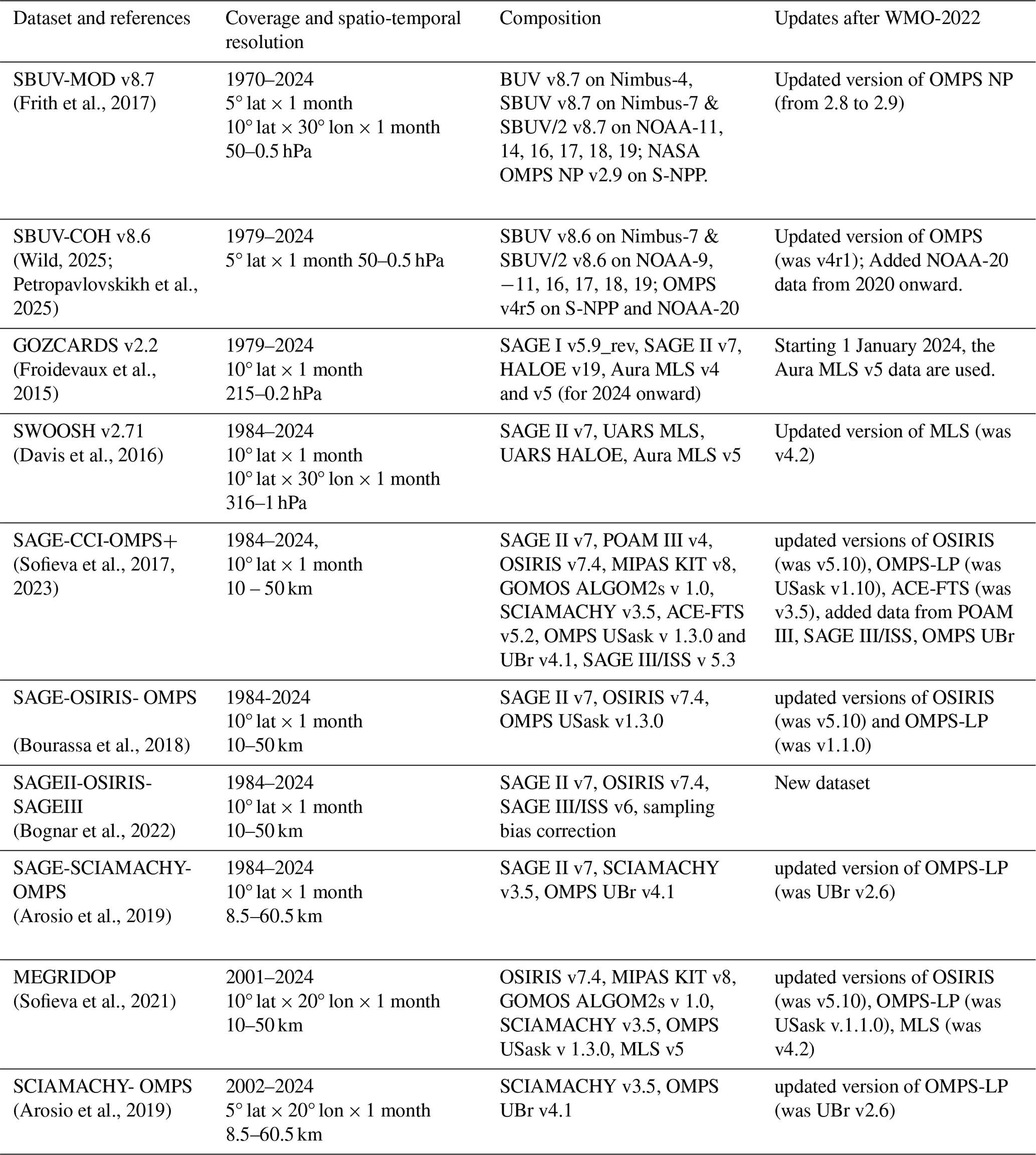
The basic information on merged satellite datasets used in our paper is collected in Table 1. In addition to the zonal mean merged satellite datasets used in GB22 and WMO-2022 – SBUV MOD, SBUV COH, GOZCARDS, SWOOSH, SAGE-CCI-OMPS, SAGE-OSIRIS-OMPS, SAGE-SCIAMACHY-OMPS – we also included a new SAGEII-OSIRIS-SAGEIII dataset (Bognar et al., 2022).

Compared to WMO-2022 (Table 1), the majority of the merged datasets used updated versions of individual satellite ozone records. The SAGE-CCI-OMPS+ dataset has been updated by including data from two additional satellite instruments – POAM III and SAGE III/ISS, and OMPS-LP profiles processed by the University of Bremen (Sofieva et al., 2023). The updated version of SBUV-COH dataset includes NOAA-processed OMPS data from both Suomi-NPP and NOAA-20 satellites. In GOZCARDS, Aura MLS v5 data are used starting 1 January 2024, as opposed to v4 data prior to this date. In fact, the ozone profiles from MLS v5 have negligible zonal mean offsets in comparison to MLS v4 (note that Aura MLS v4 data were no longer produced after 31 May 2024).

A relevant update affecting several merged limb satellite data records was the release of a new version of the Level 1 data (gridded radiances) for the Suomi NPP OMPS Limb Profiler in 2023 (Jaross, 2023). Version 2.6 includes a critical correction to the instrument altitude registration drift that was found in version 2.5. Kramarova et al. (2024) reported that the analysis of the version 2.6 ozone record demonstrated improved stability, as confirmed by the reduced relative drifts between the LP ozone and correlative measurements. The same conclusion on improved stability of OMPS-LP ozone profiles retrieved by University of Bremen was found by Arosio et al. (2024).

While some merged datasets include similar sets of satellite observations (for example, SBUV MOD and COH are created from the SBUV data, SWOOSH and GOZCARDS primarily use SAGE II  and MLS data, SAGE II data are used in six merged datasets), they still differ in the methods used to merge the original measurements as well as the exact selection of original measurements (time period, version, etc.). Comparing trend results across different merged datasets enhances confidence in the derived trend estimates.

Table 1 Information about the merged satellite datasets used in the paper.

2.2 Ground-based ozone climate data records

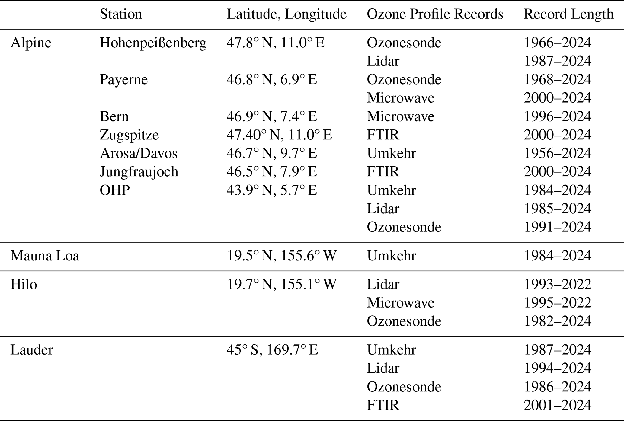
Ground-based data records used in this study are similar to those used in GB22 and have been extended to 2024 (see Table 2). Ozonesonde data have been homogenized, so that their stability is expected to be improved (Ancellet et al., 2022; Björklund et al., 2024; Van Malderen et al., 2025). The lidar ozone record at Mauna Loa stopped in 2022 due to the eruption of Mauna Loa that damaged access to the observatory (https://www.usgs.gov/volcanoes/mauna-loa/science/november-27-december-10-2022-eruption-mauna-loa, last access: 19 March 2026).

Dobson Umkehr data are derived from zenith sky observations using the optimal estimation technique (Petropavlovskikh et al., 2005, 2022). NOAA historical (up to 2020) Umkehr Dobson data were homogenized at 5 stations to remove instrumental artifacts and biases (Petropavlovskikh et al., 2022). The Arosa/Davos MeteoSwiss data record has been homogenized using colocated Brewer Umkehr records and is described in Maillard Barras et al. (2022). For this study all Umkehr data records were extended through 2024. The trends for the 2000–2020 period were analysed using the LOTUS MLR model and were found to generally agree (within uncertainty) with ozonesonde and COH overpass trends (Petropavlovskikh et al., 2025). The comparisons of the MLR and DLM trends over Arosa/Davos are summarized in Maillard Barras et al. (2022).

The three time-series at the FTIR stations (Jungfraujoch, Zugspitze, and Lauder) have been entirely reprocessed using an updated retrieval strategy as described in Björklund et al. (2024). In this study focusing on intercomparisons of many instruments measuring ozone at Lauder, it was shown that the trends using the updated and reprocessed FTIR data were more consistent with other measurements than previously reported, e.g., in GB22. The Mauna Loa microwave radiometer data record was interrupted in 2022 and resumed in January 2025 and is nevertheless used in this study. Since GB22, the Bern microwave radiometer data record has been reprocessed for harmonization with the Payerne microwave radiometer data record (Sauvageat et al., 2023).

Table 2 Ground-based ozone profile climate data records used in the analyses.

2.3 CCMI-2022 model data

Here we use data from chemistry–climate models (CCMs) participating in the CCMI-2022 experiment (https://blogs.reading.ac.uk/ccmi/ccmi-2022/, last access: 13 May 2026), which provides the most recent set of Chemistry-Climate Model Initiative (CCMI) community simulations conducted in support of the quadrennial WMO/UNEP Scientific Assessment of Ozone Depletion WMO2022.

With an aim to update projections of ozone recovery, the forcings used were specified according to recommendations from WMO (2018) and the recent Coupled Model Intercomparison Project Phase 6 (CMIP6, https://wcrp-cmip.org/cmip-phases/cmip6/, last access: 13 May 2026, Eyring et al., 2016) using the Shared Socioeconomic Pathways (SSPs) scenarios. A baseline scenario (refD2) has been developed that closely follows the specifications of the SSP2-4.5 pathway of CMIP6 (O'Neill et al., 2016), which is based upon current GHG scenarios with an intermediate future projection, and with ODSs from WMO (2018), as they were recommended at the time when CCMI-2022 simulations were performed. The ocean conditions are either modelled (from a separate climate model simulation) or internally generated (in the case of fully ocean-coupled models). The simulation includes state-of-knowledge historic forcings, with recommendations for the 11-year solar cycle and stratospheric aerosol forcings (specified as for CMIP6), with the quasi-biennial oscillation (QBO) forcing either internally model-generated or nudged from an external dataset.

This scenario (refD2), which provides a seamless simulation running from 1960 to 2100, was selected to compile a reference model dataset for comparisons with recent observations presented here, ending in 2024. Comparing this dataset to the one used in GB22, we note the differences in the number of models participating (fewer in this set), the model sources (different models), and of course in the new sets of forcings used, for both GHG and ozone scenarios, and the inclusion of stratospheric aerosol forcing.

A summary of the CCMI-2022 experiments, as well as their differences from simulations in past phases of CCMI can be found in the July 2021 SPARC Newsletter (No. 57, https://aparc-climate.org/wp-content/uploads/2025/10/SPARCnewsletter_Jul2021_web.pdf, last access: 13 May 2026).

3 The LOTUS regression model and methods for evaluation of trends

3.1 The LOTUS regression model and its updates

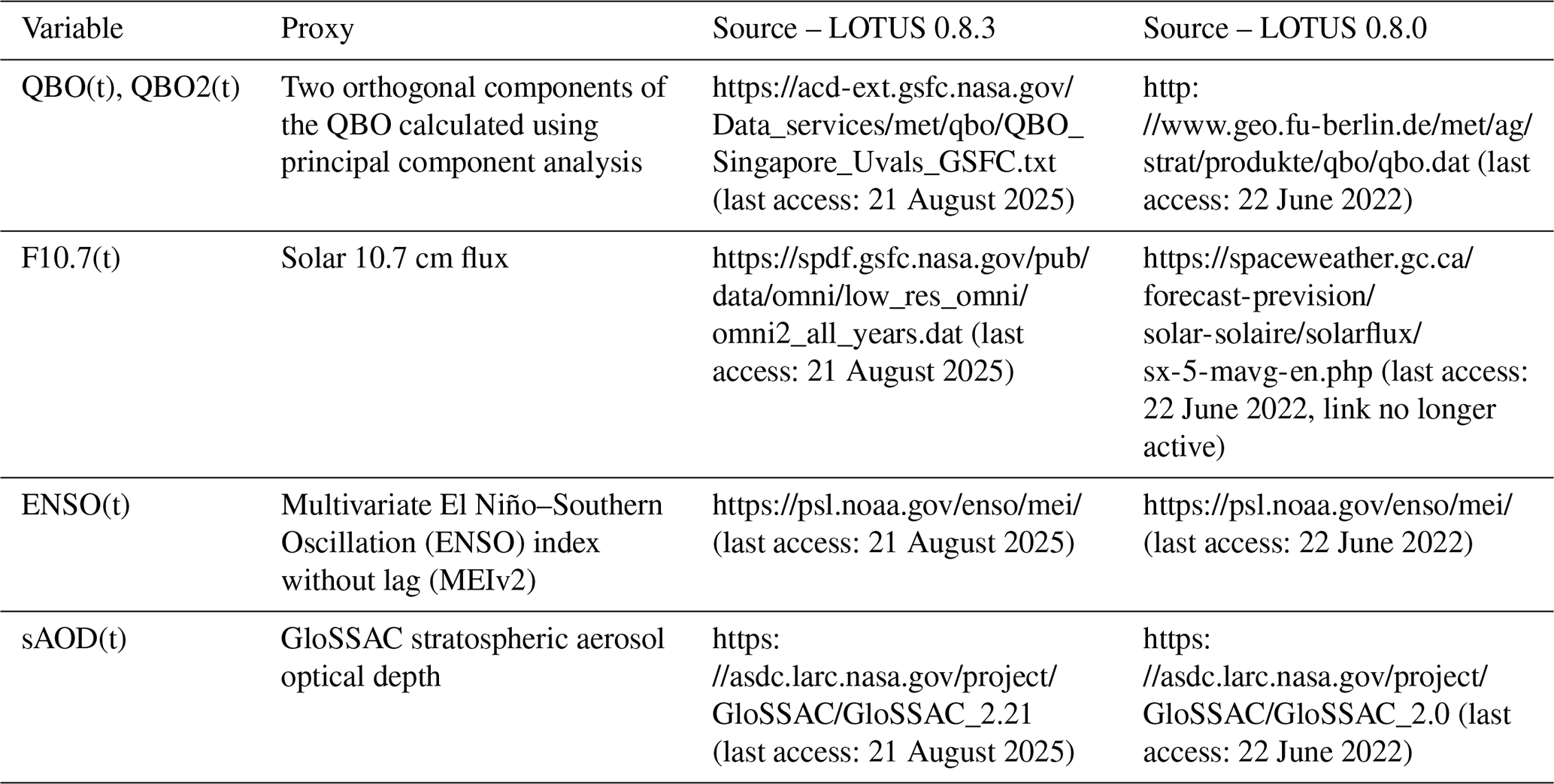
Trend analyses were performed using version 0.8.3 of the LOTUS regression model (https://usask-arg.github.io/lotus-regression/index.html, last access: 21 October 2025). This model applies a multiple linear regression framework based on the general least squares method to quantify the variability in ozone time series using several explanatory variables (proxies). The following proxies are used: QBO, El Niño-Southern Oscillation (ENSO), the 11-year solar cycle (F10.7 radio flux), and stratospheric aerosol optical depth (sAOD). Compared to LOTUS version 0.8.0 used in GB22, version 0.8.3 incorporates updated data sources for the QBO and F10.7 proxies, and the updated sAOD record (see Table 3). Following the GB22 approach, independent linear trend (ILT) terms are used to assess long-term changes before and after the peak in ozone-depleting substances (ODS), defined as January 1997 and January 2000, respectively.

For all datasets, the LOTUS regression model was applied to deseasonalized monthly mean anomalies. Datasets originally provided as monthly mean concentrations $/$ mixing ratio (ground-based data, GOZCARDS, SWOOSH, SBUV MOD and COH) were deseasonalized prior to the analysis using the 1998–2008 baseline. This deseasonalization step was omitted for the other datasets that provide de-seasonalized anomalies. The deseasonalized anomalies were then fit using the regression equation GB22:

$$\begin{array}{}\text{(1)}& \begin{array}{rl}y(z,t)& ={\mathit{\beta }}_{\mathrm{1}}(z,t)\cdot {\mathrm{QBO}}_{\mathrm{1}}\left(t\right)+{\mathit{\beta }}_{\mathrm{2}}(z,t)\cdot {\mathrm{QBO}}_{\mathrm{2}}\left(t\right)\\ & +{\mathit{\beta }}_{\mathrm{3}}(z,t)\cdot \mathrm{ENSO}\left(t\right)+{\mathit{\beta }}_{\mathrm{4}}\left(z\right)\cdot \mathrm{F}\mathrm{10.7}\left(t\right)\\ & +{\mathit{\beta }}_{\mathrm{5}}\left(z\right)\cdot \mathrm{sAOD}\left(t\right)+\left[{\mathit{\beta }}_{\mathrm{6}}\right(z)+{\mathit{\beta }}_{\mathrm{7}}(z\left)\right(t-t_{\mathrm{1}}\left)\right]\cdot L_{\mathrm{pre}}\left(t\right)\\ & +\left[{\mathit{\beta }}_{\mathrm{8}}\right(z)+{\mathit{\beta }}_{\mathrm{9}}(z\left)\right(t-t_{\mathrm{2}}\left)\right]\cdot L_{\mathrm{post}}\left(t\right)\\ & +{\mathit{\beta }}_{\mathrm{10}}\left(z\right)\cdot \mathrm{Gap}\left(t\right)+\mathit{\epsilon }(z,t),\end{array}\end{array}$$

where y(z,t) represents the monthly mean ozone anomaly at altitude z, β₁₋₁₀ are the estimated regression coefficients and ε(z,t) is the residual. The QBO is described by two orthogonal components, QBO₁ and QBO₂, derived from principal component analysis. The (independent) linear trend terms are defined as:

$$\begin{array}{}\text{(2)}& \begin{array}{rl}{L}_{\mathrm{pre}}\left(t\right)& =\left\{\begin{array}{c}\mathrm{1},t\le t_{\mathrm{1}}\\ \mathrm{0},t>t_{\mathrm{1}}\end{array}\right.L_{\mathrm{post}}\left(t\right)=\left\{\begin{array}{c}\mathrm{0},t\le t_{\mathrm{1}}\\ \mathrm{1},t>t_{\mathrm{2}}\end{array}\right.\\ & \mathrm{Gap}\left(t\right)=\left\{\begin{array}{c}\mathrm{0},t\le t_{\mathrm{1}}\\ \mathrm{1},t_{\mathrm{1}}<t\le t_{\mathrm{2}}\\ \mathrm{0},t>t_{\mathrm{2}}\end{array}\right.\end{array}\end{array}$$

where t₁ and t₂ are 1 January 1997 and 1 January 2000, respectively. The trend proxy function (Eq. 2) includes the linear terms in ozone declining (before 1997) and recovery (after 2000) period, and a constant in the “gap” from 1997–2000. Using the gap function avoids the prescription of the turnaround point, which depends on latitude and altitude (Laine et al., 2014).

To account for seasonal variability, two Fourier harmonics representing annual and semi-annual variations were applied only to the QBO and ENSO regression coefficients β_k(z,t) expressed as:

$$\begin{array}{}\text{(3)}& \begin{array}{rl}{\mathit{\beta }}_k(z,t)& ={\mathit{\beta }}_{k\mathrm{0}}\left(z\right)+{\sum }_{i=\mathrm{1}}^{\mathrm{2}}\left[{\mathit{\beta }}_{k\mathrm{1}i}\left(z\right)\sin \left({\displaystyle \frac{\mathrm{2}\mathit{\pi }it}{\mathrm{12}}}\right)\right.\\ & \left.+{\mathit{\beta }}_{k\mathrm{2}i}\left(z\right)\cos \left({\displaystyle \frac{\mathrm{2}\mathit{\pi }it}{\mathrm{12}}}\right)\right],k=\mathrm{1},\mathrm{2},\mathrm{3}\end{array}\end{array}$$

Autocorrelations were removed using the Cochrane-Orcutt transformation (Cochrane and Orcutt, 1949).

Various approaches to trend analyses are discussed in detail in P19. The analysis presented in this paper does not include attribution of ozone trends. This study is aimed at examining changes in ozone trends (a combined effect of chemistry and dynamics), derived from observations and chemistry-climate models, between two time periods, 2000–2020 and 2000–2024, and therefore we choose similar proxies and regression model settings to those used in WMO-2022.

The LOTUS model was applied to the merged satellite ozone records from 1985–2024 across all latitude bands and altitude or pressure levels, depending on the native coordinates of the datasets. The same approach was used for each vertical level of the ground-based observations at selected NDACC stations and for the gridded satellite datasets (MEGRIDOP, SWOOSH, SCIAMACHY-OMPS and SBUV-MOD) over the regions surrounding those sites. Several ground-based datasets do not cover the full period 1985–2024; therefore, the trend analysis for ground-based measurements was restricted to the period 2000–2024.

For the CCMI models, the trend analyses were performed over the period 1979–2024 using the LOTUS regression model. We calculated the appropriate QBO and El Niño–Southern Oscillation (ENSO) proxies from the model data (zonal winds and sea surface temperatures, SSTs) and used the external forcings (e.g. 11-year solar cycle) as provided to the modelling groups.

Table 3 Proxy time series used in the LOTUS regression model.

3.2 Evaluation of multi-dataset mean trends and its uncertainty

3.2.1 The mean trends for merged satellite and ground-based data

The evaluation of the mean (overall) trend from the satellite datasets follows the approach described in GB22 and P19. First, the trends from different datasets are interpolated to the same vertical grid. The combined trend $\overline{x}$ is evaluated as the arithmetic mean of the trends from individual merged datasets.

The trends from various datasets and their uncertainties cannot be considered as independent random variables: correlations of uncertainties are caused by using data from the same satellite instruments (for example, SAGE II data are used in all merged datasets except for SBUV MOD and COH; MLS data are used in both GOZCARDS and SWOOSH etc, see Table 1), and also from the natural ozone variability (common in all datasets) which is not captured by the regression model. The uncertainty of combined trends is estimated as (GB22, P19):

$$\begin{array}{}\text{(4)}& {\mathit{\sigma }}_{\mathrm{comb}}^{\mathrm{2}}=max\left({\displaystyle \frac{\mathrm{1}}{N^{\mathrm{2}}}}{\sum }_{i,j}{C}_{ij}{\mathit{\sigma }}_i{\mathit{\sigma }}_j,{\displaystyle \frac{\mathrm{1}}{n_{\mathrm{eff}}}}\sum {\displaystyle \frac{(x-\overline{x}{)}^{\mathrm{2}}}{N-\mathrm{1}}}\right)\end{array}$$

where N is the number of observation records, C_ij are the correlation coefficients for the trend estimates x_i from data sets i and j (see also below), σ_i are the trend uncertainties estimated from the fit residuals for the individual data sets, and n_eff is the effective number of independent trend estimates.

The first term in the right-hand side of Eq. (4) is the variance of the mean of correlated values, obtained through traditional propagation of errors. It serves as an approximation of the theoretical lower bound of trend uncertainty due to the actual realization of the ozone time series. The second term in the right-hand side of Eq. (4) is the unbiased estimator of the standard error of the mean. It can capture biases in trend uncertainties between the different merged data sets that would not be captured by the first term (e.g., resulting from drifts between data sets or differing unit representations). The effective number of independent values n_eff in Eq. (4) is approximated by

$$\begin{array}{}\text{(5)}& n_{\mathrm{eff}}={\displaystyle \frac{N^{\mathrm{2}}}{{\sum }_{ij}{C}_{ij}}}\end{array}$$

In Eq. (4), we do not use the sum of both terms because the variance of the trend estimates (term 2) can be partly due to the uncertainties represented by term 1. In the upper stratosphere, the second term usually dominates, while these terms have comparable values in the lower stratosphere (P19 and Fig. S7 in the Supplement).

Correlation coefficients of trend uncertainties are approximated by the correlation coefficients of fit residuals from the regression model. P19 discusses in detail the challenges of estimating the correlation of trend uncertainties, as these correspond to the largest temporal scales in the ozone time series. This approach has limitations, and the estimated correlations correspond to the upper bound of the true correlations of trend uncertainties. The values of the correlation matrix are explicitly written in the Supplement.

3.2.2 The mean trends for the models

The calculation of the CCMI-2022 multi-model mean trends follows the approach described in GB22 and P19. First, ozone data from each model were interpolated to a common zonal bin (5° latitude). Individual trends were then calculated for all models at their given pressure levels and the 5° latitude bins. In the case of multiple simulations performed by a model, the ensemble mean trend was calculated.

Final results from the CCMI-2022 models (9 in total) were averaged over the appropriate latitude bands (60–35° S, 20° S–20° N, 35–60° N), as the mean of individual model trends. Uncertainties were propagated assuming independent errors following standard rules for linear combinations (e.g., JCGM, 2008; Taylor, 1997), such that the variance of the mean equals the sum of individual variances divided by their total number squared.

4 Trend results and discussions

4.1 Zonal mean trends

Trends in vertical ozone profiles as a function of latitude are estimated using the eight merged satellite datasets, which cover the period from 1985 to 2024, with the LOTUS regression model as described in Sect. 3.1. For all datasets, the trends are evaluated using the period from 1985 to 2024. Figure 1 shows post-2000 trends as a function of latitude and pressure/altitude. Since pre-1997 data and the regression models are the same, the pre-1997 are also as in GB22, and they are not shown in our paper. The horizontal resolution and the vertical coordinates correspond to the original dataset grids. The black lines in Fig. 1 show the mean climatological thermal tropopause height (or pressure) from the ERA-5 reanalysis estimated using the post-2000 period. The trends in the upper troposphere are shaded and not assessed in this study.

For all merged datasets, positive trends of 1–4 % per decade are observed in the upper stratosphere, which are statistically significant at 95 % confidence level (this confidence level is used in all evaluations of statistical significance in our paper). The upper stratospheric trends in the Northern Hemisphere (NH), above ∼ 35 km, are larger by 1–2 % per decade for SAGE-OSIRIS-OMPS and SAGEII-OSIRIS-SAGEIII than for other merged datasets. For SAGE-OSIRIS-OMPS, slightly larger NH upper stratospheric trends were also observed in previous studies (GB22). In the lower stratosphere (∼ 7–10 km above the tropopause), nearly all datasets report negative trends in the majority of latitude zones, from −1 to −6 % per decade (depending on latitude), but the uncertainties of trend estimates are large, so that the trends are not significant (indicated by gray stippling in Fig. 1).

The morphology and magnitude of ozone trends have not changed significantly compared to the previous analyses reporting 2000–2020 trends (compare with Figs. 3–10 in WMO-2022, adapted from GB22, Fig. 1). For quantitative comparisons, we need to keep in mind that trend changes can be due to (i) extension of time period (from 2020 to 2024, including contributions from changes in atmospheric circulation or events that could have impacted ozone in the stratosphere), (ii) changes in the datasets (versioning) and (iii) changes in the trend regression model. To address these issues, we carried out sensitivity studies comparing ozone trends across old and new datasets, trend model setups, and time periods.

We found that updated data sources for the QBO and F10.7 proxies and the updated sAOD record in the regression model have a small impact on ozone trends: the differences are generally less than 0.5 % per decade with larger local deviations (up to 2 % per decade) in the UTLS (Fig. S1 in the Supplement).

The changes in 2000–2020 trends evaluated using old (as in GB22) and new versions of the merged satellite datasets are illustrated in the Supplement Fig. S2. In the middle and upper stratosphere, the changes in ozone trends due to updates in the datasets are typically less than 0.5–1 % per decade, as observed in Fig. S2. In the UTLS, especially in the tropics, the changes are larger: the trends became less negative for SAGE-CCI-OMPS+, SAGE-OSIRIS-OMPS, SAGE-SCIAMACHY-OMPS, likely due to changes in OMPS-LP version. However, the uncertainties of ozone trends in the UTLS exceed the trend estimates, so all these changes are smaller than the trend uncertainties.

The influence of the 4-year time extension on ozone trends is illustrated in Supplement Fig. S3, which compares 2000–2024 and 2000–2020 trends for individual merged satellite datasets. All datasets show a slight increase in positive trends by ∼ 1 % per decade in the middle stratosphere (10–30 hPa), mainly in the tropics and Northern Hemisphere. Some of the datasets show a slight decrease of trends in the SH upper stratosphere, by 0.5–1 % per decade. All these changes are within uncertainty intervals of the trends.

The year 2024 was characterized by high ozone values in the middle and lower stratosphere at NH mid- and high latitudes, which were associated with planetary wave events that caused significant stratospheric warmings and forced poleward and downward ozone transport into the lower stratosphere (Newman et al., 2024). When excluding this year from the time series and evaluating the trends through 2023, the ozone trends are less positive in the NH middle and low stratosphere (Figs. S4 and S5). Figure S4 also illustrates the sensitivity of trend estimates to large changes in time series at the endpoint. These changes are also within uncertainty intervals for the trends.

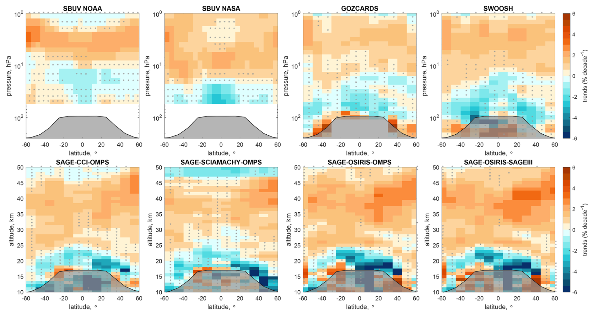
Figure 1 Ozone trends (% per decade) for the period 2000–2024 estimated from eight merged satellite data records using an independent linear trend model. Trends are shown for the SBUV COH (NOAA), SBUV MOD (NASA), SWOOSH, GOZCARDS, SAGE-CCI-OMPS, SAGE-SCIAMACHY-OMPS, SAGE-OSIRIS-OMPS, and SAGEII-OSIRIS-SAGEIII datasets. Gray stippling denotes results that are not significant at the 2σ level. Data are presented on the vertical coordinates (left-hand axis) and latitudinal grid associated with each dataset. The black lines show the mean climatological thermal tropopause height (or pressure) from the ERA-5 reanalysis. The trends in the upper troposphere are shaded and not assessed in this study.

Figure 2 presents the ozone profile trends in DU km⁻¹ per decade, for the same merged satellite datasets as in Fig. 1. The trends in absolute values are obtained from percentage trends using the climatological ozone distribution from the SAGE-CCI-OMPS+ dataset. Positive and statistically significant trends are observed in the upper stratosphere (Figs. 1–2). However, since the peak ozone abundance is in the layer ∼ 5–15 km above the tropopause, the contribution of these positive trends to changes in the total ozone column is relatively small. Ozone trends are mostly negative in the lower stratosphere (the ∼ 8–10 km layer above the tropopause), on the order of −0.2 to −0.4 DU km⁻¹ per decade, and mostly positive above this layer in the middle stratosphere, at about 0.2 to 0.4 DU km⁻¹ per decade.

Figure 2 Same as Fig. 1, but trends are expressed in DU km⁻¹ per decade.

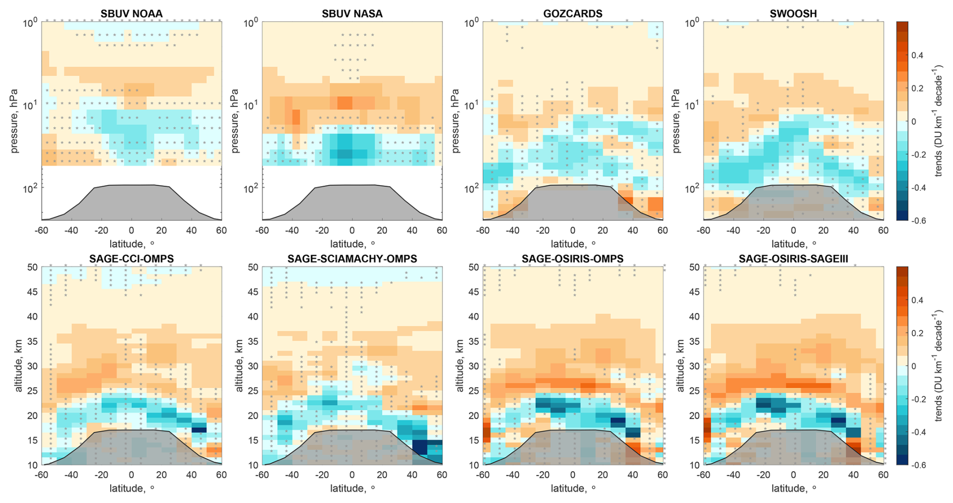
Figure 3 shows the combined (mean) trend derived from eight merged datasets as described in Sect. 3.2.1, in units of % per decade (panel a) and DU km⁻¹ per decade (panel c), with indication of its statistical significance. The combined trends shown in Fig. 3 capture the patterns in ozone profile trends that are common across the eight individual datasets analyzed in this study. Significant positive trends are observed in the upper stratosphere (35–45 km), reaching about 2–2.5 % per decade (Fig. 3a), with stronger trends at mid-latitudes. In the middle stratosphere (25–35 km), the trends are also positive but not statistically significant. In contrast, trends in the lowermost stratosphere (∼ 10–18 km in the mid-latitudes and ∼ 17–25 km in the tropics) are mostly negative, though not always significant.

When the combined trends are expressed in DU km⁻¹ per decade (Fig. 3c), the strongest positive trends of approximately 0.1 DU km⁻¹ decade⁻¹ occur in the middle stratosphere (25–35 km). Positive trends are also present in the upper stratosphere (above 35 km), but their magnitudes in DU km⁻¹ units are relatively small. Negative trends in the lower stratosphere are more pronounced, reaching about −0.2 DU km⁻¹ per decade, but they are generally not statistically significant at the 95 % confidence level.

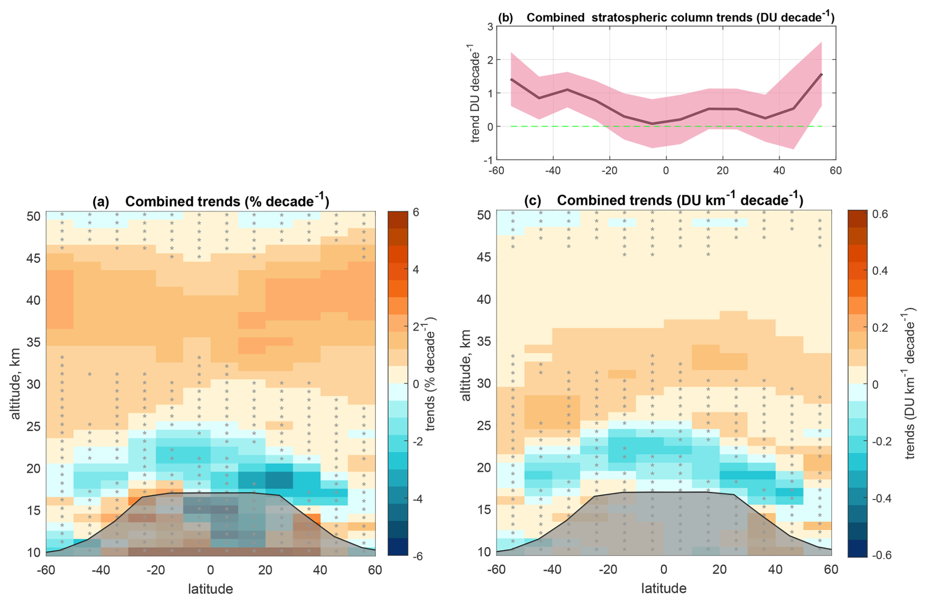
Figure 3 The combined (mean) ozone trends from eight merged satellite datasets as a function of latitude and altitude, expressed in % per decade (a) and DU km⁻¹ per decade (c). The black lines show the climatological mean tropopause height. Gray stippling denotes results that are not significant at the 2σ level. (b) stratospheric column averaged trend (DU per decade), red line, with 2σ uncertainty (pink shading). The green dashed line in panel (b) highlights zero level.

The net trend in the stratospheric ozone column (Fig. 3b) is generally positive but not statistically significant, except for the SH mid-latitudes (20–60° S) and the NH high latitudes (50–60° N), where trends are significant and reach about 1 DU decade⁻¹. In the tropics (20° S–20° N) and NH subtropics (20 –40° N), the net stratospheric column trends are smaller, around 0.1–0.5 DU per decade, and not statistically significant. The latitudinal dependence of the stratospheric ozone column trend is similar to that of total ozone column trend (WMO-2022, Weber et al., 2022) for the period from 1996 to 2020. Figure S6 in the Supplement shows stratospheric column trends as in Fig. 3b, but for different choices of end year. The variations in estimated trends are consistent with the sensitivity analyses discussed above and shown in Figs. S3–S5. Inclusion of de-trended dynamical proxies (e.g., Weber et al., 2022; Li et al., 2023; Petropavlovskikh et al., 2025) into the regression model might reduce the sensitivity of trends to the choice of the endpoint year. This can be investigated in future works.

For evaluation of trends in broad latitudinal bands (35–60° S, 20° S–20° N, 35–60° N), we used the same seven merged datasets as for GB22. The deseasonalized anomalies were first averaged in broad zones, and then the LOTUS regression model was applied. Ozone trends from individual merged datasets in broad zones are shown in Fig. 4, together with the combined (mean) trend evaluated as described in Sect. 3.2.1. All datasets report positive and statistically significant trends ∼ 2 % per decade in the upper stratosphere, with stronger trends at mid-latitudes. In the tropical lower stratosphere, all datasets report negative trends, but with large uncertainties. At mid-latitudes, the lower stratospheric trends are mostly negative with large uncertainty intervals that encompass zero trends.

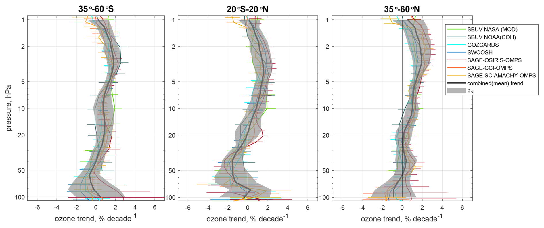
Figure 4 Ozone profile trends with 2σ uncertainties for the period 2000–2024 for latitude bands 35–60° S (left panel), 20° S–20° N (center panel), and 35–60° N (right panel). Colored lines are the trend estimates from seven individual merged datasets on their original vertical grids (SBUV NASA (MOD), SBUV NOAA (COH), GOZCARDS, SWOOSH, SAGE-OSIRIS-OMPS, SAGECCI-OMPS, and SAGE-SCIAMACHY-OMPS). Black lines represent the mean (combined) trends and gray shading indicates the 2σ uncertainty intervals for the combined trends.

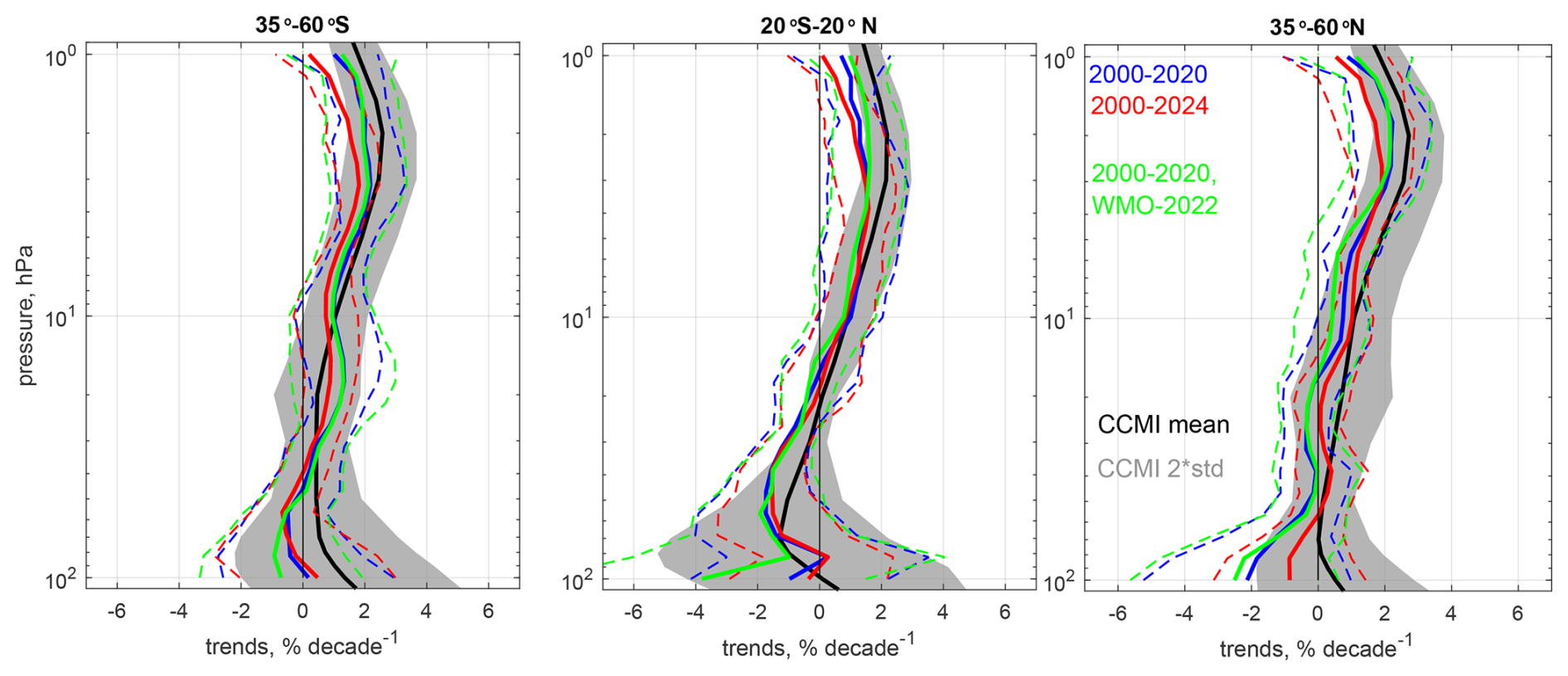
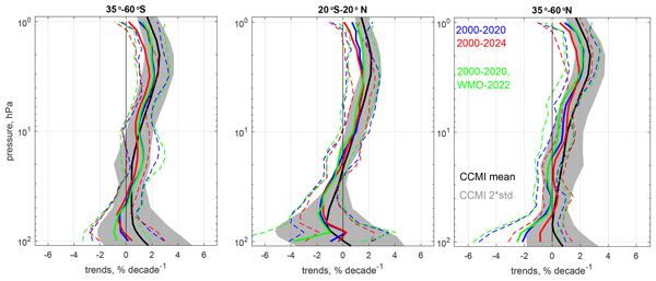
Figure 5 Comparison of simulated and observed post-2000 ozone trend profiles for the latitude bands 35–60° S (left panel), 20° S–20° N (center panel), and 35–60° N (right panel). Observed trends for the period 2000–2020 from GB22 and WMO-2022 are shown in green and the results with the updated regression model and updated datasets for the period from 2000 to 2020 and to 2024 are shown in blue and red, respectively. The mean model trends (CCMI REF-D2, 9 models) for 2000–2024 are shown in black with the 2σ uncertainties shown as shaded grey areas.

Figure 5 compares the mean ozone trends in broad latitude zones for 2000–2020 and 2000–2024 using seven merged satellite datasets (as in Fig. 4). Overall, mean trends in ozone profiles are highly consistent with the trends calculated for 2000–2020 (compare red and blue lines in Fig. 5). At mid-latitudes, a small reduction of the positive trends in the upper stratosphere by ∼ 0.5 % per decade is observed (above 10 hPa in SH and above 3 hPa in NH), though these reductions are within the estimated uncertainties. In the NH mid-latitudes, the 2000–2024 trends become more positive in the middle stratosphere (7–20 hPa) and less negative or neutral in the lower stratosphere (100–30 hPa). As discussed earlier, this is primarily due to the high NH ozone levels observed in 2024 (Newman et al., 2024). Tropical trends remain nearly unchanged. The uncertainties in the observed mean trends are slightly smaller for the 2000–2024 period, as expected due to the extended time period (see Supplement Fig. S7 for more details).

The 2000–2020 trends shown here (blue lines) have changed slightly compared to those presented in GB22 (green lines), which were also calculated over the same period. Less negative trends, on the order of 0.5–1 % per decade, are observed in the UTLS, for all latitude zones. These changes are primarily due to updates in the merged satellite ozone datasets (see Table 1) and they are consistent with the trend changes in 10° latitude bands discussed above (Fig. S2). There are no notable changes in the middle and upper stratosphere as a result of these dataset updates.

Figure 5 also shows ozone trends for 2000–2024 predicted by REF-D2 CCMI-2022 simulations (black lines for multi-model mean and grey shading for 2σ uncertainties). Since CCMI models, by design, include the key physical and chemical processes controlling ozone evolution and are driven by observation-based forcings, they reproduce observed ozone trends reasonably well. In this work, the mean CCMI ozone trends are very close to the mean satellite trends in the middle stratosphere, for all broad latitude zones. In the upper stratosphere, models predict a slightly stronger ozone recovery of +2–2.5 % per decade compared to the value from satellite observations of ∼ +1.5 % per decade. In the tropical lower stratosphere, both models and satellite observations report negative trends of ∼ −1 % per decade, but the shape of the profile trend is slightly different (but within estimated uncertainty intervals). At mid-latitudes, simulated and observational ozone trends in the lower stratosphere are now closer to each other than reported in previous evaluations (compare with Fig. 5 in GB22).

4.2 Trends over selected NDACC stations

Figure 6 shows the comparison between ground-based ozone trends over 2000 to 2024 from NDACC stations and those from combined satellite data records at three locations: (a) the SH mid-latitude site at Lauder, New Zealand; (b) the tropical sites at Hilo and Mauna Loa, Hawaii, USA; and (c) the NH mid-latitude Alpine region. In order to compare with ground-based records, we selected the MEGRIDOP, SWOOSH, SCIAMACHY-OMPS, and SBUV MOD satellite data from the nearest grid cell to the station location. Then the satellite trends were averaged to obtain a combined trend as described in Sect. 3.2.1. Alpine ground-based trends were calculated as the mean of the following records: (1) ozonesondes from Hohenpeißenberg, Payerne, and Haute Provence; (2) lidar from Hohenpeißenberg and Haute Provence; (3) Umkehr from Arosa/Davos and Haute Provence; (4) FTIR from Zugspitze and Jungfraujoch; (5) MWR from Payerne and Bern. In the Alpine region, ozone trends are evaluated for each station and instrument type  separately and then averaged by instrument type.

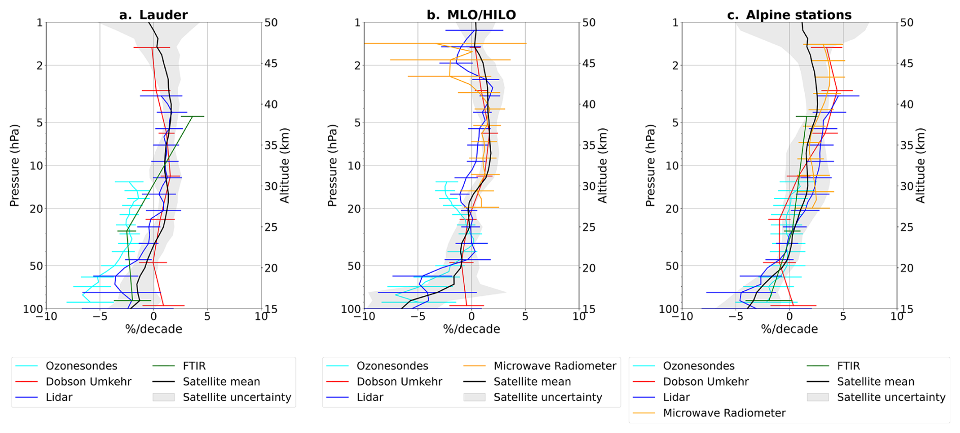
Figure 6 Ozone trend profiles (% per decade) for 2000 to 2024 at selected NDACC locations: (a) Lauder (New Zealand); (b) Mauna Loa and Hilo (Hawaii, USA); (c) Alpine stations that include (1) ozonesondes from Hohenpeißenberg, Payerne, and Haute Provence; (2) lidars from Hohenpeißenberg and Haute Provence; (3) Umkehr from Arosa and Haute Provence; (4) FTIR from Zugspitze and Jungfraujoch; (5) MWR in Payerne and Bern. Trend profiles are shown for ozonesondes (light blue), Dobson Umkehrs (red), lidars (dark blue), microwave radiometers (orange), and FTIR (green). For lidars, microwave radiometers and ozonesondes error bars are plotted every 2nd step for clarity. Also shown is the mean satellite trend profile, estimated by averaging MEGRIDOP, SWOOSH, SCIAMACHY-OMPS, and SBUV-MOD satellite data from the nearest grid boxes. Error bars represent the 95 % confidence intervals.

It should be noted that the FTIR ozone profiles have a relatively low-vertical resolution (only about 3 Degrees of Freedom for Signal in the stratosphere (Vigouroux et al., 2015)), therefore the FTIR trends plotted in Fig. 6 represent ozone changes in wide partial columns 12–20, 20–29, and 29–48 km.

Overall, the agreement between the ground-based and combined satellite trends is good, the trends mostly remain within uncertainty intervals. Note that the spatio-temporal sampling patterns are different for ground-based and satellite measurements, thus contributing to trend differences (the representativeness of climate data records from ground-based instruments is discussed in e.g. Zerefos et al., 2018; Björklund et al., 2024). The largest discrepancies in trends from different GB instruments at a single location occur at Lauder but have been significantly reduced compared to GB22.

The Lauder station (Fig. 6a) shows negative trends from −2.5 to −6 % per decade in the lower stratosphere (below 20–25 km) and positive trends of up to 1.3 % per decade in the upper stratosphere (above about 35 km). The trends from Dobson Umkehr and lidar data agree well with the combined satellite trends, while ozonesondes show stronger decline in the lower stratosphere. Ozonesonde trends are outside the satellite mean uncertainty range. A similar discrepancy was reported in GB22 (Fig. 4 in GB22) with even stronger negative trends from ozonesondes at Lauder. Zeng et al. (2024) reported that homogenization of ozonesonde data at Lauder has a small impact on post-2000 trends. The analyses of drifts between climate data records from different instruments at Lauder by Björklund et al. (2024) have explained roughly half of them by the different sampling, vertical sensitivity, or time periods and gaps. Especially, in the lower stratosphere the drifts between FTIR, sondes and Lidar partial columns (14–22 km) were found below 1 % per decade.

At the Mauna Loa/Hilo site (Fig. 6b), positive trends of up to 1.5 % per decade are observed in the upper stratosphere, while negative trends appear in the lower stratosphere (up to −6 % per decade). The instruments are largely consistent, though the lidar measurements show smaller positive or even slightly negative trends in the middle stratosphere (25–35 km). Note that the Mauna Loa lidar and MWR data records end at the end of 2022 due to the Mauna Loa volcanic eruption.

The Alpine stations (Fig. 6c) show strong positive trends in the upper stratosphere, reaching +2.5 to +4 % per decade, and negative trends of up to −4 % per decade in the lower stratosphere. Above 45 km, the trends remain positive but decrease. Overall, the Alpine sites exhibit the strongest positive trends in the upper stratosphere and the weakest negative trends in the lower stratosphere among all stations. The agreement across different instrument techniques is the best among the three selected study cases. The combination of multiple Alpine records has a smoothing effect, which might also contribute to this good agreement.

In general, for all stations, the trends from ground-based measurements are consistent with the satellite mean trends (black line) and capture the same overall vertical pattern of ozone trends. They show ozone recovery in the upper stratosphere, weaker or transitioning trends from negative to positive in the middle stratosphere, and negative trends in the lower stratosphere. Compared to Fig. 4 in GB22, the agreement between ground-based and satellite measurements has improved (e.g., for the FTIR at Lauder), but there are still differences (e.g., ozonesonde trends at Lauder and Umkehr trends in various locations in the lowermost stratosphere). The uncertainties of the trends from ground-based instruments are also reduced compared to GB22, particularly in the lower stratosphere. Trends in the upper stratosphere differ only slightly (< 1 % per decade), while the lower stratospheric ground-based trends are less negative compared to GB22. These changes remain within the ground-based trend uncertainties.

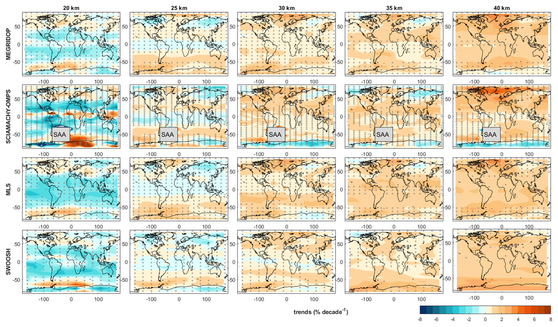
Figure 7 Latitude- and longitude-dependent ozone trends (% per decade) derived for the period 2003–2024 for five different altitude levels, based on the extended MEGRIDOP, SCIAMACHY-OMPS, SWOOSH, and MLS datasets. Gray dots indicate regions where the trends are not statistically significant at the 2σ level. For the SCIAMACHY-OMPS dataset, ozone trends in the Southern Atlantic Anomaly (SAA) region are not shown because SCIAMACHY data are flagged in this region.

4.3 Global regional trends

For evaluation of regional trends, we used the three currently available merged high-vertical-resolution datasets with resolved longitudinal structure: MEGRIDOP, SCIAMACHY-OMPS and SWOOSH. Similarly to Sofieva et al. (2021), we selected the years after 2003 for trend analyses, in order to avoid the influence of major sudden stratospheric warming in September 2002 on ozone trends at Southern Hemisphere middle and high latitudes. Figure 7 shows the horizontal structure of ozone trends in the period 2003–2024 at 5 altitude levels: 20, 25, 30, 35, and 40 km. In addition to the aforementioned datasets, we also show trends from the MLS dataset (evaluated using the period 2004–2024). The trends are evaluated using the same setup of the multiple linear regression model, but with a single linear trend term due to the shorter time period.

A strong longitudinal dependence of ozone trends in the NH extratropics (at latitudes poleward of 50° N) and below 40 km is observed. The trends are characterized by a dipole-like structure with positive trends over Scandinavia and negative trends over Siberia, which had been reported by Arosio et al. (2019) and Sofieva et al. (2021) based on the 2003–2018 time period. Arosio et al. (2024) has shown that model simulations also reproduce this pattern in ozone trends. The study concludes that this zonal asymmetry is primarily driven by dynamical processes, such as a weakening and shift in the activity of planetary wavenumber-1 over the past two decades (Arosio et al., 2024).

The magnitude of both positive and negative trends in the dipole-like patterns over the NH has slightly decreased compared to the earlier studies by Arosio et al. (2019) and Sofieva et al. (2021). At the same time, lower stratospheric (around 20 km) trends in the SH (20–55° S) are more zonally uniform now with predominantly negative but insignificant trends. The patchy positive values in the SCIAMACHY+OMPS data set in the inner-tropical lower stratosphere are caused by Hunga-Tonga aerosol-related artifacts in the UV/VIS satellite ozone retrieval.

A small negative trend has emerged over Antarctica above 40–45 km (seen primarily in SCIAMACHY-OMPS); however, this negative trend is not statistically significant. Since natural variability is high in polar regions, it is quite expected that a simple multiple regression gives trend estimates that are not statistically significant and sensitive to the selected (or available) time period. Other methods for trend analysis in polar regions, such as considering seasonal trend (Galytska et al., 2019; Solomon et al., 2016; Szeląg et al., 2020), using dynamical proxies (e.g., Weber et al., 2022) or vortex-related coordinates can be explored in future works.

5 Summary

In this paper, we presented an updated analysis of trends in stratospheric ozone profiles in the latitude range 60° S–60° N using long-term ground-based and merged satellite climate data records, including a comparison with chemistry-transport models.

The ground-based datasets include the climate data records constructed from ozonesonde, lidar, FTIR, Dobson Umkehr, and microwave radiometer data. Satellite climate data records include eight merged datasets with zonally averaged profiles: SBUV MOD, SBUV COH, GOZCARDS, SWOOSH, SAGE-CCI-OMPS+, SAGE-SCIAMACHY-OMPS, SAGE-OSIRIS-OMPS and SAGEII-OSIRIS-SAGEIII. In addition, regional trends are estimated using the merged satellite datasets with resolved longitudinal structure: MEGRIDOP, SCIAMACHY-OMPS, and SWOOSH. Most datasets have been updated since GB22 and WMO-2022 by incorporating new versions of existing satellite datasets, adding new satellites, and other developments.

The trends in ozone profiles have been evaluated using the LOTUS multiple linear regression model with QBO, ENSO, solar flux and aerosol proxies and independent-linear terms for trends. The whole time series starting from 1985 are used for trend evaluation, but only post-2000 trends are discussed in this paper. The method of Petropavlovskikh et al. (2019) is applied to estimate the overall combined trends and uncertainties from the satellite data. The paper presents a detailed characterization of global (zonally averaged and in broad latitude zones) and regional (with resolved longitudinal structure) ozone trends, in both relative and absolute units, from individual climate data records as well as the overall combined trends.

Overall, the mean trends in ozone profiles over 2000–2024 are highly consistent with the trends calculated over 2000–2020 and reported in WMO-2022 and references therein. Our analyses of satellite data confirm the statistically significant positive ozone trends in the upper stratosphere ∼ 1–3 % per decade, with larger trends at mid-latitudes compared to the tropics. Compared to WMO-2022, the upper stratospheric trends are nearly unchanged in the tropics but are slightly reduced at mid-latitudes. The 2000–2024 trends in the NH middle stratosphere are more positive compared to the 2000–2020 trends, partly due to the high NH ozone levels in 2024. In the lower stratosphere, the trends are mostly negative, −1–2 % per decade. Compared to the 2000–2020 period, the lower stratospheric trends are nearly unchanged in the tropics and SH mid-latitudes, but they became less negative at NH mid-latitudes, again primarily due to high NH ozone levels in 2024.

Ozone trends predicted by REF-D2 CCMI simulations in the period 2000–2024 are in very close agreement with the mean satellite trends in the middle stratosphere, for all broad latitude zones. In the upper stratosphere, models predict a slightly stronger ozone recovery of +2–2.5 % per decade than observations. In the lower stratosphere, both models and satellite observations report negative tropical trends of ∼ −1 % per decade, while modelled ozone trends are slightly positive at mid-latitudes. However, simulated and observational ozone trends in the mid-latitude lower stratosphere are now closer to each other than reported in GB22 and WMO-2022. All estimated trends in the lower stratosphere have large uncertainties, and they are not statistically significant.

Ozone profile trends over several stations estimated from ground-based records generally agree with the trends estimated using merged satellite datasets with resolved longitudinal structure. We found a good agreement between trends from ground-based and satellite measurements in the tropics and in the Alpine stations, while trend values for different types of ground-based instruments are more scattered at the Lauder station (but nevertheless improved compared to WMO-2022).

The analysis of regional ozone profile trends in 2003–2024 using merged satellite datasets confirmed the previous observations of a longitudinal structure in ozone trends in the NH mid-latitude stratosphere, with positive trends over Scandinavia and negative trends over Siberia. However, the magnitude of this dipole-like structure is reduced due to extension of the data records. The estimated regional trends are consistent with the zonally averaged trends.

Maintaining well-calibrated, merged ozone records and conducting periodic assessments of ozone trends are essential for reliably tracking the uneven recovery of the ozone layer and comparing observations with predictions from chemistry–climate models, especially in the face of emerging disruptions such as major volcanic eruptions, extreme wildfires, increasing greenhouse gas concentrations, and increased satellite debris. As key satellite missions approach the end of their lifetimes, the risk of observational gaps is growing, particularly for critical stratospheric species (e.g., water vapor, chlorine species, N2O) that are needed to interpret changes in ozone. A reduced number of correlative satellite observations will undermine our ability to rapidly identify anomalies and instrumental drifts, leading to increased uncertainties in merged records and derived trends. In this context, the role of the ground-based network becomes even more important, both for satellite validation and for independent assessments of regional ozone variability and long-term change.