Annual cycle of surface-coupling effects on Arctic mixed-phase clouds during MOSAiC

Persistent mixed-phase clouds frequently occur in the Arctic and have significant impacts on the Arctic climate. The surface mixed-layer (SML) coupling status of these clouds impacts their microphysical properties. Here, the annual cycle of Arctic mixed-phase cloud ice-formation temperatures is presented for the Arctic ice-drift experiment Multidisciplinary drifting Observatory for the Study of Arctic Climate (MOSAiC) in 2019 and 2020. From October until March, no clouds with cloud minimum temperatures above −10 °C were observed. From April to September, an increased fraction of ice-containing clouds was observed for clouds with minimum temperatures between −7.5 and −5 °C (between 40 % and 70 %). Between April and July, SML-coupled clouds with a minimum temperature above −7.5 °C showed an enhanced fraction of ice-containing clouds, compared to decoupled clouds (2–3 times higher). Also, SML-coupled clouds were 2–4 times more likely to be observed during this period. In August + September the ratio of coupled-to-decoupled ice-containing clouds reduced to 1.3, due to a higher frequency of occurrence of ice-containing decoupled clouds. Using surface-based ice-nucleating particle (INP) measurements the observed phenomena could likely be attributed to the presence of INPs active above −15 °C at the surface. Analysis of sea-ice concentration in the surrounding region, the distance to the ice edge, and back-trajectory residence time above sea ice supports this finding.

1 Introduction

Ice formation in mixed-phase clouds, clouds which consist of liquid-droplets and ice-crystals at the same time, plays a critical role in the complex processes which are modulating the cloud properties, precipitation formation, their radiative effect, and cloud lifetime (e.g., Curry et al., 1996; Morrison et al., 2012). The phase partitioning in mixed-phase clouds is closely interlinked with turbulence, the humidity supply, and the availability of cloud-relevant aerosol particles, such as ice-nucleating particles (INPs) and cloud condensation nuclei (CCN) (Morrison et al., 2012; Kalesse et al., 2016; Radenz et al., 2021). Ice formation in clouds in the so-called heterogeneous temperature regime, i.e., approximately down to −38 °C, is initiated by INPs (Hoose and Möhler, 2012), a rare subset of all aerosol particles in the atmosphere. Observations as well as model studies showed that deviations in INPs and CCN concentrations have significant impact on the liquid- and ice-microphysical properties and thus the radiative effect of the cloud (Curry, 1995; Prenni et al., 2007). Adding more CCN can decrease the droplet size, increase the liquid water path (LWP) and decrease the ice water path (IWP), while an increase in INPs can increase the IWP with decreasing LWP (Morrison et al., 2008). The Arctic ocean, with a strong dependence on the ice cover, is a source for moisture and heat, but also for aerosol particles, in the lower Arctic troposphere (Curry et al., 1995; Uttal et al., 2002; Held et al., 2011; Schmale et al., 2021; Shupe et al., 2022). A factor that controls the relevance of these surface sources for cloud properties is the thermodynamic state of the lower troposphere, i.e., the coupling between cloud and surface (Brooks et al., 2017; Gierens et al., 2020; Griesche et al., 2021).

The probability of INP activation depends on its composition and temperature, increasing with decreasing temperature. Dust particles are globally one of the most prominent INPs below −15 °C (Ansmann et al., 2009; Seifert et al., 2010; Murray et al., 2012; Kanji et al., 2017; Villanueva et al., 2025). Above −15 °C, ice formation is usually associated with INPs containing biogenic material (Pereira Freitas et al., 2023; Hartmann et al., 2025). In the Arctic, INPs can be advected into the Arctic via long-range transport or they originate from local sources, e.g., sea spray aerosol, local dust emissions from glacial outwash, or local primary biological activity (DeMott et al., 2016; Šantl Temkiv et al., 2019; Si et al., 2019; Tobo et al., 2019; Creamean et al., 2020; Ansmann et al., 2023; Wieber et al., 2025). Highly active INPs have been found close to melting sea ice and in melt water samples (Wilson et al., 2015; Irish et al., 2017; Zeppenfeld et al., 2019; Mavis et al., 2025), in airborne samples collected over polynyas (Hartmann et al., 2020), as well as close to the North Pole (Porter et al., 2022). Creamean et al. (2022) presented the annual cycle of surface INP concentrations in the high Arctic ocean from the Multidisciplinary drifting Observatory for the Study of Arctic Climate (MOSAiC) expedition and highlighted a maximum of INPs active above −15 °C during summer. During winter and spring, the dominating INP sources were long-range transported, while during the melt season in summer biogenic particles likely originated from more local sources. Still, biogenic material was found in the INP samples throughout the whole year (Barry et al., 2025). Based on ship-based lidar observations made during MOSAiC, Ansmann et al. (2023) presented an annual cycle of aerosol optical properties and CCN and INP concentrations in the boundary layer and the free troposphere. The INP concentrations were higher during summer and a shift of the dominating ice-forming particle type from dust particles in winter to sea spray aerosol in summer was identified. While recent work has started to evaluate in situ vertical distributions of INPs in the below- and in-cloud environment to directly assess what INPs may affect cloud ice formation, most measurements still occur at the surface which presents a disconnect in the often-stratified Arctic boundary layer (e.g., Creamean et al., 2021; Griesche et al., 2021; Porter et al., 2022; Ansmann et al., 2023; Pilz et al., 2024; Böhmländer et al., 2025).

A significant feature of Arctic mixed-phase clouds is the formation of a shallow liquid-dominated layer at cloud top. Strong radiative cooling at cloud top drives convection within the cloud (Shupe et al., 2008; Tjernström et al., 2012; Egerer et al., 2019; Lonardi et al., 2022), initiating feedback loops, e.g,. via continuous droplet formation, that help to maintain the cloud (Morrison et al., 2012). This convection can generate an exchange of the cloud with a mixed-layer below cloud base (Brooks et al., 2017). If this cloud mixed-layer (CML) reaches the turbulent surface mixed-layer (SML), surface properties may influence the cloud properties by acting as source of moisture and cloud-relevant aerosol particles (Eirund et al., 2019; Gierens et al., 2020; Griesche et al., 2021; Radenz et al., 2021). Using radiosonde and tethered ballon profiles, Akansu et al. (2023) showed that under cloudy conditions the SML usually is deeper. The CML and the SML together are denoted here as planetary boundary layer (PBL), which is usually capped by a temperature inversion, most of the time located at cloud top (Brooks et al., 2017). Above Arctic mixed-phase clouds specific humidity inversions were regularly observed, which can serve as additional resupply for moisture via cloud top entrainment (Sedlar et al., 2012; Neggers et al., 2019; Egerer et al., 2021). Also, cloud relevant particles in the free troposphere, e.g., from long-range transport can be entrained downward into the PBL (Igel et al., 2017; Solomon et al., 2018). Jimenez et al. (2025) showed that ice formation in free-tropospheric Arctic mixed-phase clouds is dominated by immersion freezing. Due to persistent observed droplet formation, the authors concluded that the free Arctic tropospheric CCN and INP reservoir is unlikely to be depleted, and the dissipation of the observed clouds was rather due to insufficient water vapor supply. Silber and Shupe (2022) analyzed radiosonde data during MOSAiC and found in 73 % of the profiles a liquid-containing cloud layer. In about 51 % of the profiles the authors reported multiple liquid-containing cloud layers.

Substantial research has been conducted on the influence of the coupling between the CML and SML on mixed-phase cloud properties. Jozef et al. (2024) analyzed MOSAiC radiosonde profiles and found stronger tropospheric stability during winter and spring, and least stability during fall. During summer they observed similar occurrences of both cases, strong stability and weak stability. The authors hypothesized that a stronger stability may lead to more decoupled cases, while a weaker stability supports SML-coupling. Creamean et al. (2021) used tethered balloon observations to investigate the vertical aerosol distribution in the Arctic PBL. The authors found, that only in 14 % of the analyzed profiles, the aerosol particles were uniformly mixed between the surface and the cloud base. Using INP filter samples and trajectory analysis, Ohneiser et al. (2026) showed for two pre-Alpine sites, one in the free troposphere, one in the PBL, that the resupply of INPs from the free troposphere may be limited due to the stability at the top of the PBL. The INP concentration in the free troposphere was higher, compared to the one in the PBL. Using ground-based remote sensing at the Arctic site Ny-Ålesund, Svalbard, Gierens et al. (2020) observed enhanced liquid water path (LWP) in coupled clouds. Based on a combination of ground-based remote sensing, radiosonde profiles, and satellite-based sea-ice information, Saavedra Garfias et al. (2023) showed that the water vapor transport (WVT) from sea-ice leads influences the cloud properties. Clouds coupled to the WVT from sea ice leads in the central Arctic, i.e., when the maximum of the vertical gradient of WVT was located within the CML, showed a larger liquid fraction, lower cloud base, and a larger vertical extend (Saavedra Garfias et al., 2023). Papakonstantinou-Presvelou et al. (2022) found an increased ice-crystal number concentration in clouds that have been observed over the Arctic sea-ice, compared to clouds above the open ocean, based on 10 years of satellite remote sensing. Above both surface types the ice-crystal numbers were increased, when only coupled clouds were considered. Griesche et al. (2021) analyzed ship-based remote sensing of clouds from a two month expedition in the high Arctic. The authors showed, if clouds were thermodynamically coupled to the surface, they contained ice more frequently, especially at temperatures above −15 °C. They argued that this phenomenon is likely due to a local source of INPs containing biogenic material, which were transported into the clouds when the PBL was well mixed. Such biogenic material can include, among others, polysaccharides and proteins emitted from the ocean. Marine polysaccharides, in particular, have recently been shown to act as efficient ice-nucleating molecules (Hartmann et al., 2025) and to reach high altitudes up to the free troposphere, as demonstrated by a recent balloon study in Ny-Ålesund (Zeppenfeld et al., 2025). Yet, there are still missing links between cloud relevant particles, the surface, and clouds. INP measurements are limited in the Arctic and still often surface-based, profiles are even more sparse. It is not entirely clear how and under which circumstances the observed INP load actually may impact cloud properties. Also the responses of the PBL and of clouds to the changing surface conditions in the Arctic are not yet fully determined.

Riming, ice-crystal and liquid-droplet collision, as well as aggregation, ice-crystal and ice-crystal collision, are two major contributors to the ice mass in Arctic mixed-phase clouds (Chellini et al., 2022; Maherndl et al., 2024). Using ground-based remote sensing of clouds at Ny-Ålesund, Svalbard, Chellini and Kneifel (2024) identified turbulence as a relevant factor for aggregation and riming of ice particles between −20 and −10 °C and argued that this also increases secondary ice production (SIP). SIP has been shown to play a substantial role in Arctic mixed-phase clouds by tethered-ballon borne observations made in Svalbard (Pasquier et al., 2022). Radenz et al. (2021) showed that gravity waves forced by the orography along the trajectory of the air mass, influence the ice occurrence at temperatures below −15 °C. The occurrence of low-level clouds in the Arctic typically increases during spring time, which was, based on space-borne lidar observations, attributed to an enhanced fraction of liquid-containing mixed-phase clouds on the expense of pure-ice clouds (Lac et al., 2026). Yet, certain aspects of some underlying mechanisms controlling Arctic mixed-phase clouds are still under discussion and models struggle, for example, to reproduce the observed cloud annual cycle, the relative distribution of liquid and ice, especially in low-level clouds, (Taylor et al., 2019; Wei et al., 2021; Shaw et al., 2022), and the role of aerosol particles in Arctic cloud processes (Schmale et al., 2021; Kiszler et al., 2024).

The presented study is a follow up of Griesche et al. (2021), using an entire year of observations in the Arctic ocean. We use data from the year-long Arctic ice-drift expedition MOSAiC (Shupe et al., 2022). The MOSAiC expedition took place from September 2019 until October 2020 and aimed to observe a full annual cycle of the Arctic system. MOSAiC was based on the German icebreaker Polarstern, which was located in the central Arctic for the whole period, except for a small interruption end of May until beginning of June 2020, where the sea ice was left for a crew rotation. Continuous ground-based remote sensing from cloud radar and lidar was used to identify clouds and classify their phase and vertical extent (Engelmann et al., 2021; Shupe et al., 2022; Griesche et al., 2024b). By means of radiosonde profiles the SML-coupling state of the cloud and the cloud-minimum temperature were derived. Additionally, in situ observations of INPs, Hybrid Single-Particle Lagrangian Integrated Trajectory model (HYSPLIT, Stein et al., 2015) back-trajectory analyses, and sea-ice conditions from satellite observations were used to constrain links between the coupling-state of the cloud and surface properties.

(Engelmann et al., 2016)(Engelmann et al., 2025)(Engelmann et al., 2025)(Kollias et al., 2016)(Lindenmaier et al., 2024)(Lindenmaier et al., 2024)(Creamean et al., 2025)(Hill et al., 2024)(Jensen et al., 2016)(Dahlke et al., 2023)(Dahlke et al., 2023)(Dahlke et al., 2023)

Table 1 Applied instruments and their specifications. ν represents the respective applied frequency of the instrument and λ the wavelength. R indicates the measurement range and P the precision of the measured quantity. T specifies the respective temporal resolution and V the vertical resolution.

2 Instrumentation

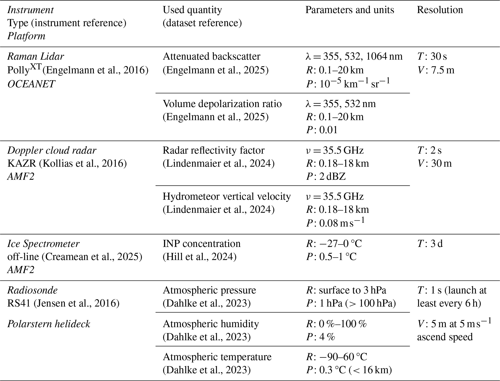
This study is based on a combination of ground-based remote sensing and different in situ measurements, which are summarized in Table 1.

2.1 Ground-based remote sensing

One of the remote-sensing facilities operated during MOSAiC was the OCEANET-Atmosphere (hereafter referred to as OCEANET) container from the Leibniz-Institute for Tropospheric Research TROPOS, Leipzig, Germany (Engelmann et al., 2021; Griesche et al., 2024b). The mobile platform OCEANET has previously been operated on different research vessels and earlier voyages (Kanitz et al., 2013; Bohlmann et al., 2018; Griesche et al., 2020), and based for one year in Antarctica at the German Neumayer Station III (Radenz et al., 2024).

During MOSAiC, OCEANET comprised a multiwavelength depolarization Raman lidar Polly^XT, two microwave radiometers, two disdrometers, as well as a terrestrial and a solar radiation sensor. Polly^XT measures elastic backscattered light at 355, 532, and 1064 nm with a complete overlap in 700 m (Engelmann et al., 2016). Additional near range receiver are included for 355 and 532 nm with a complete overlap in 120 m. Raman-capabilities are implemented for, e.g., water vapor retrievals (Seidel et al., 2025). Finally, depolarization information was retrieved at 355 and 532 nm. The measurement from Polly^XT were averaged to 30 s profiles with a vertical resolution of 7.5 m.

Another remote-sensing platform operated during the MOSAiC expedition was the Atmospheric Radiation Measurement (ARM) mobile facility 2 (AMF2) from the United States (US) Department of Energy. The AMF2 was equipped with, among others, different lidar and cloud radar systems, and a wind profiler. For this study the Ka-band ARM Zenith cloud radar (KAZR) was utilized, which operates at 35 GHz. The KAZR was operated with a temporal resolution of 2 s and a vertical resolution of 30 m. The KAZR provided measurements of the radar reflectivity factor, the hydrometeor vertical velocity and the width of the Doppler spectrum.

The combined remote-sensing dataset was, for example, used to derive continuous, height-resolved cloud microphysical cloud properties for the entire MOSAiC year (Engelmann et al., 2025), as described in Griesche et al. (2024a), based on the synergistic instrument approach of Cloudnet (Illingworth et al., 2007; Tukiainen et al., 2020). This dataset contains, among others, a pixel-based target classification of the cloud phase. The liquid-water detection within Cloudnet is based on the lidar measurements. The ice-detection is based on the temperature (no ice at T > 0 °C) and a falling pixel identified by the cloud radar. See Hogan and O'Connor (2004) for more details on the Cloudnet target classification in general and Griesche et al. (2024b) for the MOSAiC Cloudnet data set.

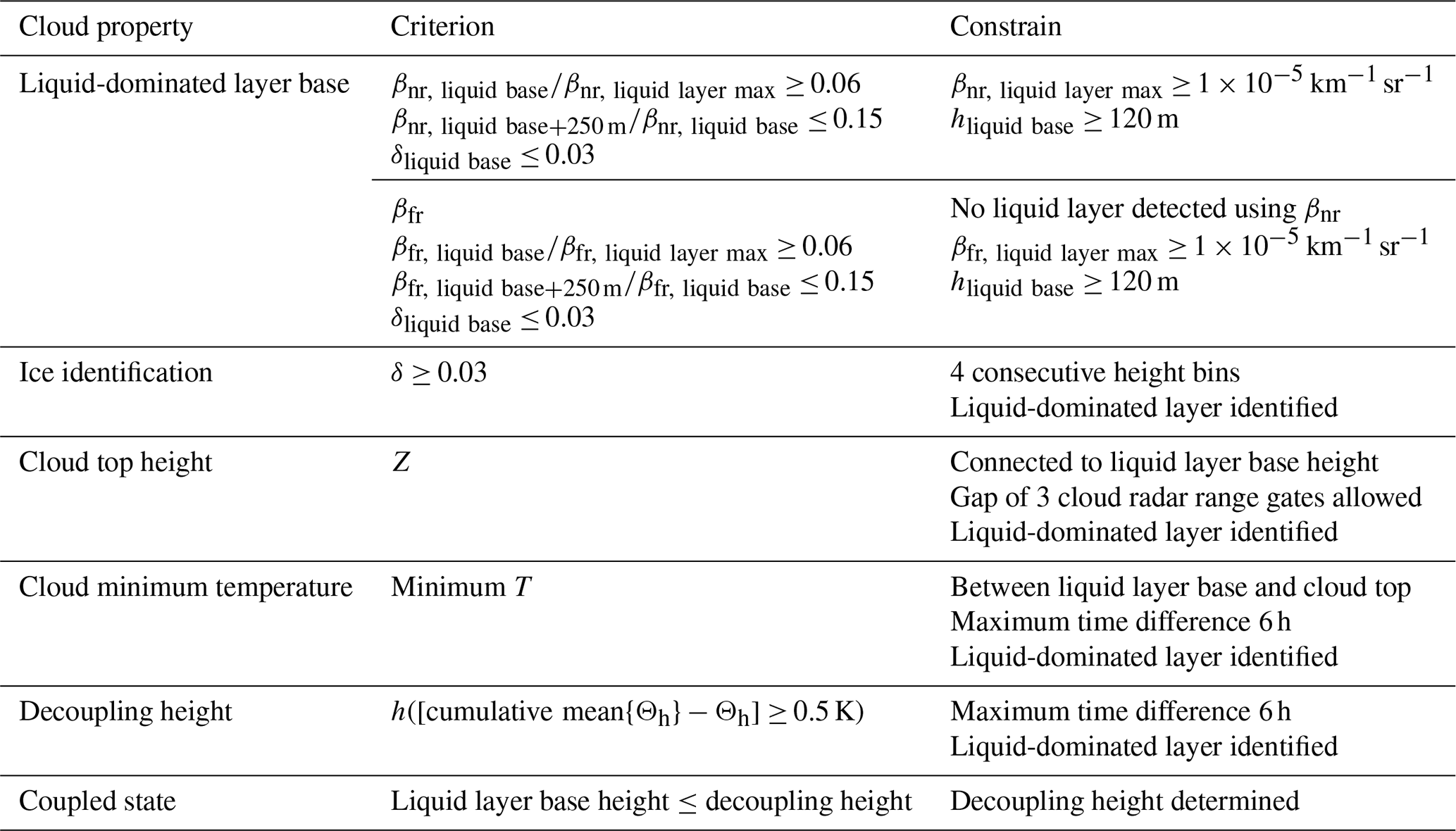
Table 2 Summary of the approaches and thresholds for cloud property identification.

2.2 INP data

In situ measurements were also performed with the AMF2 platform during MOSAiC. A filter sampler was installed approximately at 15 m above sea level for INP sampling. INP filters on Polarstern were changed roughly every 3 d and were analyzed after the expedition at Colorado State University (CSU), US, using the Ice Spectrometer (IS). Details on the methodology and dataset can be found in Barry et al. (2025). For INP sampling, 0.2 µm pore polycarbonate filters were used. Based on theoretical collection efficiencies (Spurny and Lodge, 1972), it is assumed that the total suspended particulates were collected. The collection efficiency varies with size of the collected particles and has its minimum at about 0.1 µm (about 80 %).

2.3 Radiosonde profiling

In situ profiles of thermodynamic state of the whole tropospheric column were derived using radiosondes, which were launched at least every 6 h during the entire year. These profiles provide atmospheric pressure, humidity, and temperature up to the stratosphere.

3 Methodology

To study the influence of cloud SML-coupling on the ice occurrence, a stepwise analysis of the data was performed. Initially, the remote-sensing data were checked for a liquid-dominated layer base. In case of a detected liquid-dominated layer base, the corresponding cloud phase (liquid-only or ice-containing), cloud top height, and cloud minimum temperature were determined. Finally, the respective SML-coupling state (coupled or decoupled) of the cloud was identified. The whole analysis was done on data averaged to the 30 s resolution of the lidar data. The respective procedure is introduced in detail in the following subsections and all criteria and constraints are summarized in Table 2. Based on the results of the cloud identification, the fraction of ice-containing clouds was derived. Following Seifert et al. (2010) the standard error σ was calculated using

$$\begin{array}{}\text{(1)}& \mathit{\sigma }=\sqrt{f(\mathrm{1}-f)/n},\end{array}$$

with f the fraction of ice-containing clouds and n the hours of clouds observations. The standard error is indicated in the statistics of fraction of ice-containing clouds as uncertainty bars.

The observations were analyzed for two months each, starting from October 2019 until end of September 2020, in order to retrieve sufficient statistics of the fraction of ice-containing clouds during the MOSAiC year. In Fig. 1 the respective parts of the MOSAiC expedition track for each 2-month period are highlighted. Finally, INP and back-trajectory analyses were done.

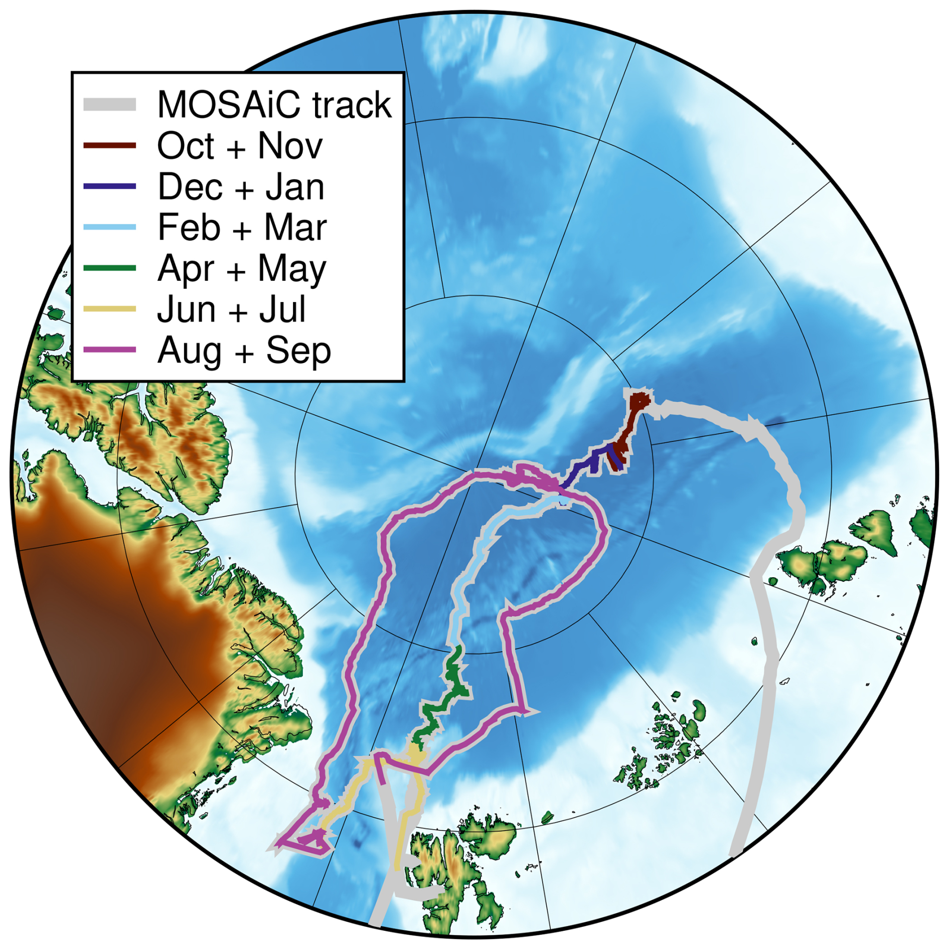
Figure 1 Track during the MOSAiC expedition (gray line). The different colored lines shows the part of the track Polarstern drifted during each 2-month period analyzed in Fig. 5. The map was created with PyGMT (Tian et al., 2023).

3.1 Liquid identification and cloud ice detection

The lidar, due to its sensitivity to the number of particles in a sample volume, was primarily used for the identification of liquid-dominated layers. Only liquid-dominated layer base heights higher than 120 m were considered in the analysis, to account for the impact of the optical overlap of the lidar system on the signal profiles. The procedure for detecting liquid-dominated layers follows Jimenez et al. (2020), which relied on normalized attenuated backscatter β_norm = $\mathit{\beta }/{\mathit{\beta }}_{\text{max}}$. To identify a liquid-containing cloud β_norm should exceed a threshold of β_{norm,  max} = 0.06. As in Jimenez et al. (2020), a 5-bin smoothing was applied to minimize the effect of signal noise on the detection algorithm. This approach was developed for clouds in the free troposphere higher than 500 m, while this study focuses on low-level, SML-coupled clouds. Hence, additional constraining criteria were applied to the liquid-layer detection. The volume depolarization δ and β profiles were used to avoid misclassification of backscatter signals. For a liquid-containing cloud identification, δ should not exceed a value of 0.03. The additional criteria for the attenuated backscatter profile were as follows: The maximum of the attenuated backscatter β_max should exceed a value of 1 × 10⁻⁵ ${\mathrm{sr}}^{-\mathrm{1}}{\mathrm{km}}^{-\mathrm{1}}$ and the signal should decrease by at least 85 % within 250 m above the liquid-containing layer due to the strong attenuation by the droplets. The introduced liquid-layer detection approach was first applied to the near range channel of the Polly^XT system. If no liquid-containing layer was found in the near range data, the far range signal was analyzed.

For ice identification a threshold of δ_ice = 0.03 was applied to the lidar volume depolarization ratio δ. δ_ice was theoretically derived by considering the lowest detectable ice water content from a lidar of 10⁻⁶ kg m⁻³ (Bühl et al., 2013). The detailed derivation of the threshold is outlined in Appendix A. Each depolarization ratio profile was screened for δ≥δ_ice. For an ice-containing cloud, the depolarization ratio profile should exceed δ_ice for at least 4 consecutive lidar height bins (= 30 m) below the liquid layer base. The cloud phase determination was done my means of the lidar, though the cloud radar is actually more sensitive to ice particles. However, the cloud radar has its lowest usable range gate in 180 m above the instrument.

3.2 Cloud top and minimum temperature, and surface mixed-layer coupling

The cloud top height was derived from the cloud radar reflectivity Z and was set to the highest altitude, where Z was continuously connected to the liquid-dominated layer base. To account for small inhomogeneities in the clouds, a gap of 3 cloud radar range gates (= 90 m) was allowed. The cloud minimum temperature was set to the lowest temperature between liquid-dominated base and cloud top from the closest radiosonde profile within 6 h of the observed cloud profile.

The SML-coupling was derived following Gierens et al. (2020), using the potential temperature Θ derived from measurements of the temporally closest radiosonde. The height where the difference between the cumulative mean of Θ and Θ exceeded 0.5 K was set as the respective decoupling height. If the decoupling height was below the liquid-dominated base, the cloud was considered as decoupled. A quasi constant Θ profile until cloud base and hence a decoupling height above the liquid-dominated base was classified as coupled. Same as for the cloud minimum temperature, only cases within 6 h before or after a radiosonde launch were considered.

3.3 Fraction of ice-containing clouds

For each 2-months period between October 2019 and September 2020, the clouds were categorized by their cloud minimum temperature in temperature intervals, separated at T = [−40, −35, −30, −25, −20, −15, −10, −7.5, −5, −2.5, 0] °C. For the entire MOSAiC period, this analysis was done for all clouds. For the late spring and summer months, i.e., for April + May, June + July, and August + September, the clouds were further analyzed based on their coupling state.

3.4 INP concentration

Surface-based INP filter measurements from CSU (Hill et al., 2024) were used to investigate a possible connection between elevated INP concentrations at the ground and ice formation in the clouds. INP filter collection and analysis is described in detail by Barry et al. (2025) and is only briefly outlined here. Filters were prepared and collected following ultraclean procedures to ensure sample integrity as described by Barry et al. (2021). During MOSAiC, the sampling setup included a totalizing mass flow meter, vacuum pump, tubing, and precipitation shield. Filters were typically collected for 72 h, totaling to an average of 88 000 sL (standard liters) of air per filter. After collection, filters were stored and shipped frozen until analysis at CSU.

For analysis, the CSU IS was used (e.g., Creamean et al., 2025). Particles were re-suspended from filters into 7–10 mL of 0.1 µm-filtered deionized water in sterile 50 mL tubes and rotated for 20 min to ensure mixing. Each IS consists of two 96-well aluminum blocks encased by cold plates, with two instruments run in parallel. Aliquots of 50 µL were dispensed into four sterile 96-well polymerase chain reaction (PCR) plates using up to five 11–15-fold serial dilutions. Plates were sealed in the IS, purged with HEPA-filtered N₂, and cooled at 0.33 °C min⁻¹ while freezing is recorded every 0.5 °C. The detection limit ranged from −27 to −29 °C depending on the deionized water blanks. INP number concentrations were calculated following Vali (1971) from the fraction of frozen droplets, volume of sample suspension, and total air volume filtered.

3.5 Trajectory analysis

Back-trajectories were calculated using the transport and dispersion model HYSPLIT (Stein et al., 2015). 5 d trajectories were initialized every hour at the liquid-dominated base of the analyzed clouds. The back-trajectories were used to derive the residence time above sea ice for the observed clouds, calculated as the time between observation and ice edge. The ice edge is defined as SIC below 50 % in a 50 km radius around the trajectory location or if within the 50 km radius 50 % of the area was above land.

3.6 Sea ice properties

To investigate the influence of different sea ice conditions on the cloud properties the sea ice concentration (SIC), the lead fraction, and melt-pond fraction were analyzed. The SIC was derived from the satellite-based merged MODIS and AMSR2 dataset with a resolution of 1 km from the University of Bremen (Ludwig et al., 2019, 2020). During the MOSAiC period, this dataset, however, is only available until end of May 2020. Hence, from beginning of June 2020 SIC from the AMRS2 data (Spreen et al., 2008) with a resolution of 3.125 km was used. The lead fraction was taken from the satellite synthetic-aperture radar derived sea ice divergence based on Sentinel-1 data (von Albedyll, 2024) as described in von Albedyll et al. (2024). Lead fraction data covers the period between October 2019 and May 2020, with a gap between 14 January and 15 March 2020 when Polarstern was north of the maximum latitude of Sentinel-1. The melt-pond fraction was obtained from the Ocean and Land Colour Instrument (OLCI) data on board the Sentinel-3 satellite as described in Istomina et al. (2025).

Both, SIC and lead fraction were derived within a radius of 50 km around Polarstern. The melt-pond fraction was derived in an area of 100 km around Polarstern because the melt-pond data coverage is reduced in summer. Additionally, the melt pond fraction was only calculated if the coverage of valid data points within the 100 km radius was above 10 %.

3.7 Eddy dissipation rates

Eddy dissipation rates (EDR) were derived based on the cloud radar hydrometeor vertical velocity, following Griesche et al. (2020). To estimate the EDR turbulence spectra from 5 min cloud radar Doppler time series were used. If, in a log-log representation, the turbulence spectrum follows a $-\mathrm{5}/\mathrm{3}$ slope within its inertial subrange, the EDR ϵ was calculated using

$$\begin{array}{}\text{(2)}& \mathit{ϵ}={\left({\displaystyle \frac{{\mathrm{10}}^{k_{\mathrm{0}}}}{A}}\right)}^{\mathrm{3}/\mathrm{2}},\end{array}$$

with A=0.5 the Kolmogorov constant and k₀ the intercept of the of the linearized fit within the inertial subrange. Deviations up to 20 % of the $-\mathrm{5}/\mathrm{3}$ slope (i.e., $-\mathrm{5}/\mathrm{3}$ ± $\mathrm{1}/\mathrm{3}$) were accepted.

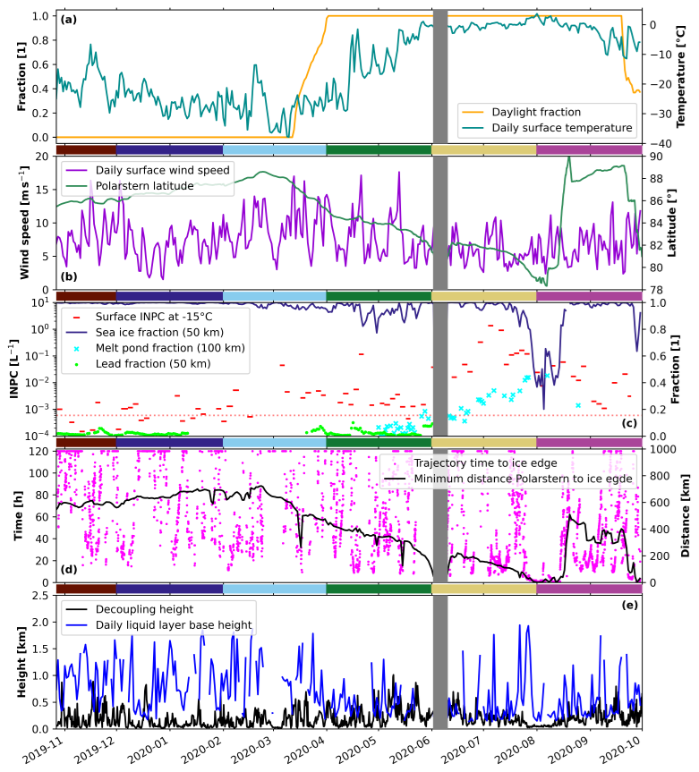
Figure 2 Overview of the MOSAiC expedition period. Panel (a) shows the theoretical daylight fraction at the position of Polarstern (orange) and the observed daily averaged surface temperature (green). In panel (b) daily averages of the surface wind (purple) and Polarstern latitude (dark green) are depicted. Panel (c) highlights the sea ice fraction (dark blue: 50 km radius), the melt pond fraction (cyan crosses: 100 km radius), and the lead fraction (green dots: 50 km radius) around Polarstern. In addition, the concentration of INPs active at −15 °C measured at the surface is depicted by the red bars. The red dotted line in panel (c) marks the 30th percentile of the INP concentrations. In panel (d) the time in hours the backward trajectories started at the liquid layer base needed to reach the ice edge is shown by the pink dots. The black line in panel (d) shows the minimum distance of Polarstern to the ice edge. The derived decoupling height (black) and daily averaged liquid layer base height (blue) are shown in panel (e). The gray shaded period in each panel marks the period where Polarstern left the sea ice for a crew rotation between 2 June 2020 and 10 June 2020. The brown, blue, orange, green, red, and purple bars between the panels highlight the analyzed periods in Fig. 5.

4 Results

4.1 Campaign overview of atmospheric and surface conditions

An overview of atmospheric and surface properties at the Polarstern site during MOSAiC is shown in Fig. 2. Three distinct warm-air intrusions (WAI) can be identified in the temperature evolution (blue line in Fig. 2a). The first WAI reached Polarstern during mid-end of November 2019, with temperatures at the surface above −10 °C. The second WAI occurred mid-end of February 2020 with surface temperatures slightly below −10 °C, and the last one during mid-end of April 2020 with temperatures close to 0 °C (Dada et al., 2022; Kirbus et al., 2023). Dada et al. (2022) showed that the April WAI had a significant impact on the aerosol size distribution and chemical composition. The WAI introduced a change of the atmospheric aerosol conditions in the Arctic from a Arctic haze dominated state into a more polluted state. Kirbus et al. (2023) highlighted that the warm air during this WAI was advected via two different pathways. A first intrusion starting on 15 April originated in northwestern Russia and passed the Barents Sea, while the second intrusion starting on 18 April was advected via west of Svalbard. Filter samples collected subsequent to each WAI showed elevated INP concentrations, compared to filter samples collected before the WAI (red bars in Fig. 2c).

From November 2019 until March 2020 the surface INP concentration shown in Fig. 2c increased slowly from around 5 × 10⁻⁴ to around 1 × 10⁻² L⁻¹. Between March 2020 and end of May 2020 the INP concentration was rather constant. Two filter samples stand out during this period, the first after the February WAI beginning of March and the one following the April WAI with values of 4 × 10⁻² and 1 × 10⁻¹ L⁻¹, respectively. In June the INP concentration increased quickly from 1 × 10⁻² to up to 10 L⁻¹ beginning of July, followed by a slow decrease again. Though, these measurements were the first ones reported for mid-winter for the central Arctic, other observations carried out at land-based stations or late-winter (March) were on the same order of magnitude close to 3 × 10⁻⁴ L⁻¹ (Wex et al., 2019; Hartmann et al., 2020). The summer-peak values during MOSAiC in early July were about one order of magnitude higher compared to simultaneously performed measurements at Zeppelin station on Ny-Ålesund (Barry et al., 2025). At that time, there was a distance of about 450 km between both sites.

The SIC remained close to 100 % with only minor variations until mid April 2020. In late April 2020 the SIC went occasionally down to less than 80 %, which was, however, attributed to wet snow rather than open water (Krumpen et al., 2021). A rapid decrease of the SIC with values below 40 % was observed towards end of July 2020 when the ice floe reached the ice edge. With the relocation of Polarstern to a new floe mid of August 2020, the SIC in the vicinity of Polarstern increased again to around 100 %. The highest lead fraction in the vicinity of Polarstern was 10 % on 16 April 2020 during the April WAI. However, most of the time the lead fraction was below 2 %. The melt-pond fraction increased strongly from close to 0 % during mid of May 2020 to more than 40 % in August and September 2020. Rapid variability in the distance to the ice edge shown in panel (d) can be caused, for instance, by the opening of large leads or polynyas, as for example on 16 March 2020.

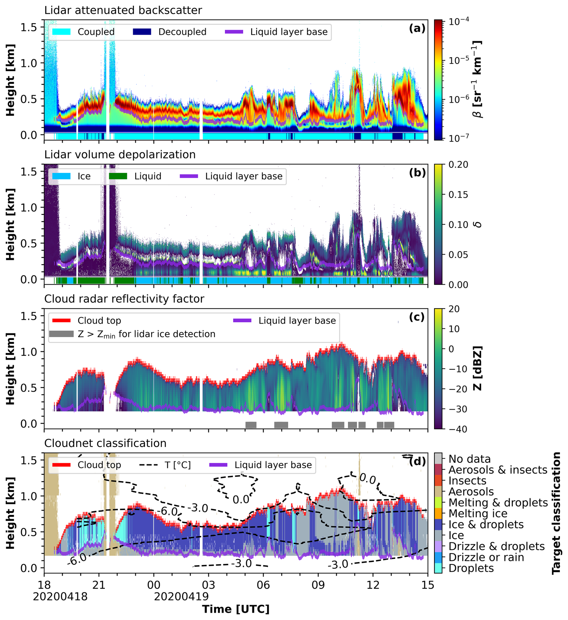
Figure 3 Ground-based remote sensing of lidar attenuated backscatter (a) and lidar volume depolarization (b), cloud radar reflectivity factor (c), and Cloudnet target classification (d) for the period of 18 April 2020 18:00 UTC to 19 April 2020 15:00 UTC. In all panels additionally the liquid-dominated layer base (purple line) is shown (a 7 bin smoothing was applied for clarity reasons). The light (coupled) and dark blue (decoupled) bars at the bottom of panel (a) show the respective coupling state. In panel (b) additionally the derived cloud phase depicted by the blue (ice-containing) and green (liquid) bars at the bottom. The red line in panel (c) and (d) shows the cloud top height and the gray bars at the bottom of panel (c) highlight periods where the cloud radar reflectivity factor met the theoretical threshold of lidar ice detection. In panel (d) the temperature is indicated by the dashed isotherms.

The daily averaged liquid-dominated layer base height depicted by the blue line in Fig. 2 panel (e) showed a strong variability throughout the year. It was highest during winter and spring and lowest during early summer. In late summer mostly very low values were observed. The derived decoupling height (black line) is lower during winter and higher during summer. However, also during winter conditions where the clouds were coupled to the SML can be identified.

4.2 Case study: ice formation at temperatures just below −5 °C

Figure 3 shows a case study of a persistent low-level stratus cloud observed above between 18 April 2020–18:00 UTC and 19 April 2020–15:00 UTC. This cloud occurred during the second intrusion of the April 2020 WAI, with air mass advection from the North Atlantic (Kirbus et al., 2023). Within this cloud, ice formation at temperatures slightly below −5 °C was observed. The observed cloud was continuously below 1 km height and identified as SML-coupled cloud, except for short periods on 19 April 2020, between 06:00 and 08:00 UTC and again between 11:00 and 14:00 UTC when some variations in the liquid-dominated layer base were observed. Ice-containing clouds were identified by enhanced depolarization values below the liquid-dominated layer base (purple line), as for example most of the time from 18 April 2020 23:00 UTC until 19 April 2020 08:00 UTC. In Fig. 3c, those periods that revealed a cloud radar reflectivity and hence ice occurrence which was high enough to a produce a signal which should be detectable by the lidar are highlighted by the gray bars below the plot. The threshold reflectivity was derived based on the findings from Bühl et al. (2013) and the IWC-Z-T relationship presented in Hogan et al. (2006). Note, however, that the lowest detection limit of the lidar is lower than the one from the cloud radar and that the lidar may also detect ice production below the lowest detection range of the cloud radar. Hence, there can be periods where the lidar identified an ice-containing cloud but the cloud radar reflectivity was actually below the limit for lidar-based ice detection. The radar reflectivity in Fig. 3c reveals that the derived liquid-dominated layer base (purple line) was frequently below the lowest range gate of the cloud radar (e.g., on 19 April 2020 between 01:00 and 02:00 UTC and later on that day between 05:00 and 09:00 UTC and between 11:00 and 15:00 UTC).

Back-trajectories for the cloud depicted in Fig. 3 are shown in Fig 4. Note, while an ensemble of 27 trajectories was initialized every hour, only one trajectory of the ensemble and only for every second hour is shown for clarity reasons. The respective location of each trajectory of the ensemble at the ice edge is marked in the same color as the trajectory. If the residence time above sea ice was less than 15 h the location where the trajectory hit the ice edge was marked with a cross, when the residence time was more than 15 h it was marked with a circle. The location where the single trajectory ensemble members reached the ice edge can vary and hence the derived residence time. For example, some of the trajectories initialized on 18 April 2020, 20:00 UTC (shown in purple) reached the ice edge in less than 15 h (indicated by the purple crosses), while other ensemble members needed more than 15 h (indicated by the purple circles).

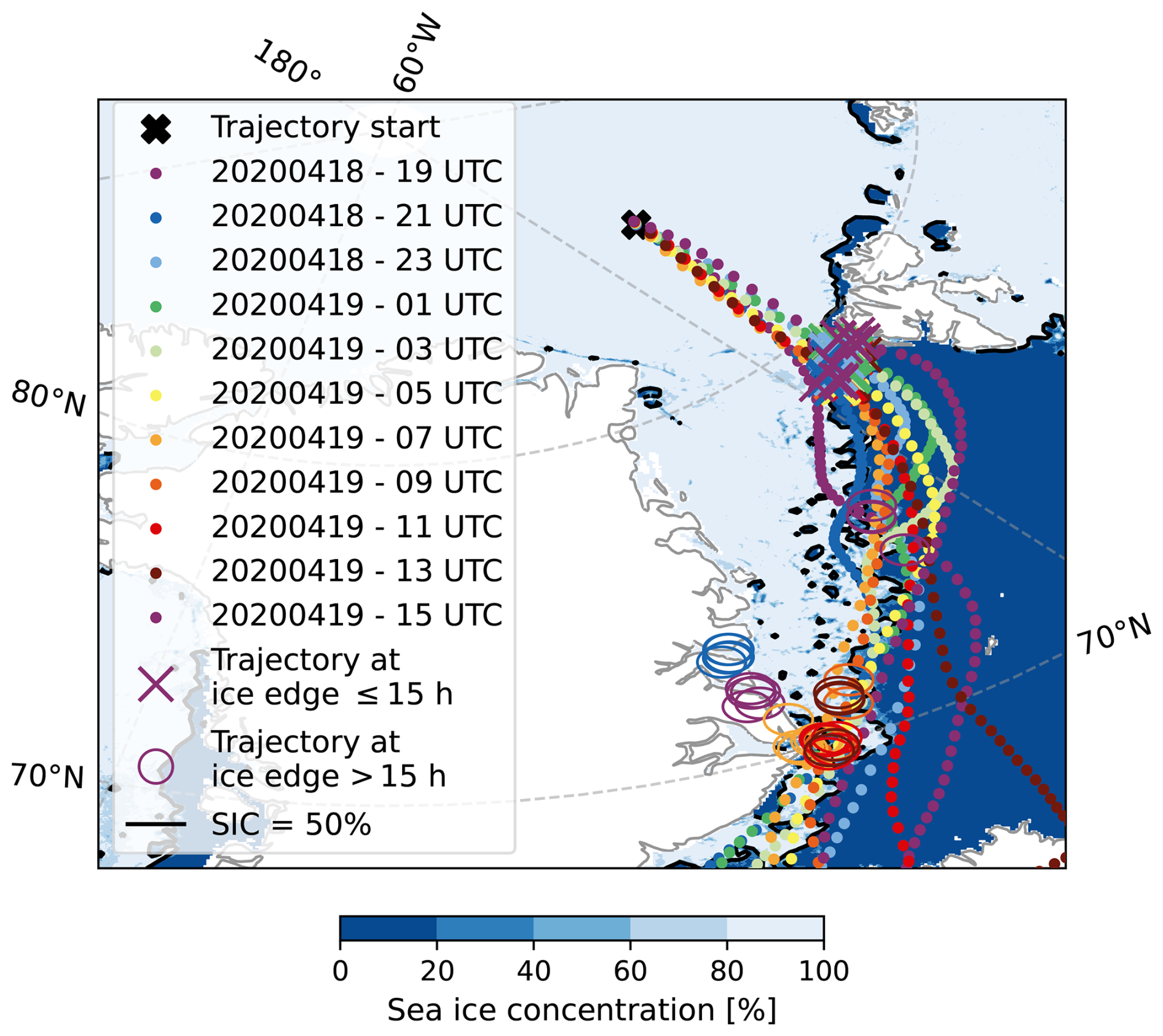
Figure 4 Back-trajectories for the cloud presented in Fig. 3. For each member of the ensemble the location where the trajectory reached the ice edge is marked with a cross (less than 15 h residence time) or a circle (more than 15 h residence time). The background shows the sea ice concentration on 18 April 2020.

4.3 Fraction of ice-containing clouds

4.3.1 Annual cycle

In Fig. 5 the fraction of ice-containing clouds as a function of their minimum temperature during the MOSAiC expedition for two months each is presented. The numbers above the plot indicate the hours of cloud observations used to derive the fraction of ice-containing clouds in the respective temperature interval during the 2-month periods in the same color codes. The errors bars show the statistical uncertainty as in Seifert et al. (2010).

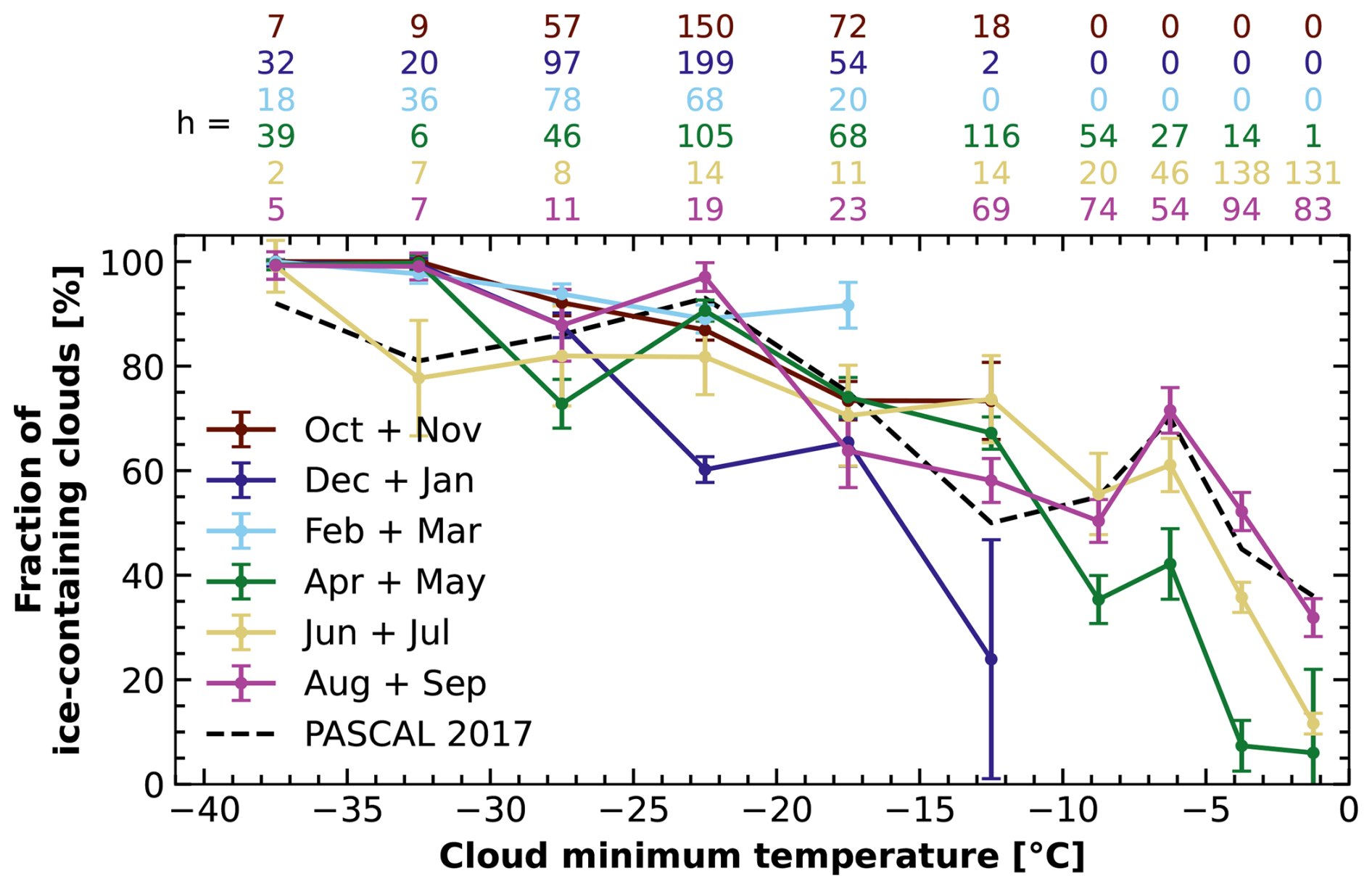
Figure 5 Fraction of ice-containing clouds observed at different cloud minimum temperature intervals during the MOSAiC year. Each colored line represents a 2-month period and the black dashed line shows the fraction of ice-containing clouds observed over the Arctic ocean in summer 2017 (Griesche et al., 2021). The numbers above the plot highlight the hours of cloud observation used in the respective temperature interval in each 2-month period.

In October + November 2019 (brown) during 18 h of observations and in December 2019 + January 2020 (dark blue) during 2 h of observations, clouds with a liquid-dominated layer and a cloud minimum temperature between −15 and −10 °C were observed, but no clouds at temperatures above −10 °C. In February + March 2020 (light blue) no clouds with minimum temperatures above −15 °C were detected. In April + May 2020 (green), an enhanced fraction of ice-containing clouds with a minimum temperature above −15 °C was observed, with a peak between −7.5 and −5 °C of 40 %. This peak corresponds to 27 h of observation. The fraction of ice-containing clouds increased through June + July 2020 (yellow, 60 %, 46 h of observation) until August + September 2020 (pink) with a distinct peak of about 70 % between −7.5 and −5 °C cloud minimum temperature from 54 h of observations. For each 2-month period between April and September, this peak is followed by a minimum between −10 and −7.5 °C and then a steady increase with decreasing temperature close to 100 % of ice-containing clouds. These findings follow the results from Griesche et al. (2021), as indicated by the dashed black line in Fig. 5.

4.3.2 Coupling effects

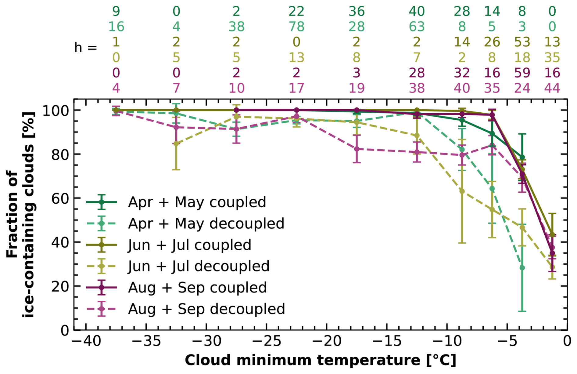
Figure 6 shows the same as Fig. 5 but for the months April + May , June + July , and August + September separated into coupled and decoupled clouds. The coupling analysis shows that the increased fraction of ice-containing clouds in April + May and June + July at low-supercooling temperatures can mostly be attributed to clouds coupled to the SML. In April + May and at cloud minimum temperatures between −7.5 and −5 °C, coupled clouds were observed during 22 h and 45 % of the time these clouds were identified as ice-containing. Only during 5 h of observation in April + May decoupled clouds were identified, with 20 % ice-containing. For June + July, decoupled clouds between −7.5 and −5 °C were found to contain ice up to 25 % of the time, whereas 70 % of the coupled clouds in this temperature range were ice-containing. Decoupled clouds in June + July were observed during 11 h and coupled clouds during 35 h. In August + September, the difference between coupled and decoupled clouds between −7.5 and −5 °C in terms of ice fraction but also in hours of observation changed, due to an increased fraction of decoupled ice-containing clouds. Under SML-coupled conditions, ice was found in 85 % of the clouds observed in August + September, which relates to 17 h of observation. Decoupled situations were observed during 37 h and in 65 % of the time ice-containing clouds were identified.

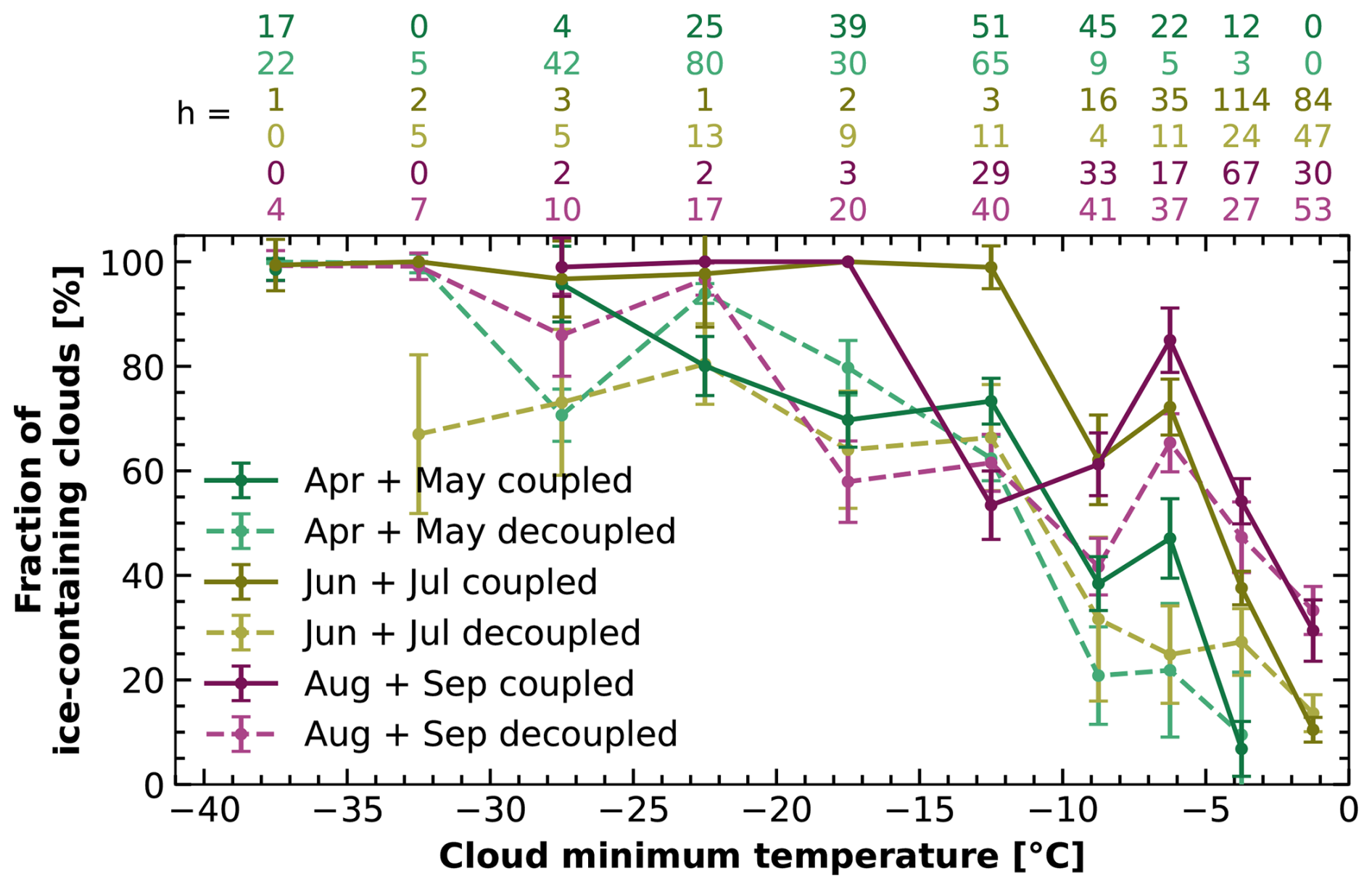
Figure 6 Same as Fig. 5 but only for April + May (light and dark green), June + July (light and dark yellow) and August + September (light and dark purple). The observations of each 2-month period are separated by their coupling state, with the continuous lines and darker colors showing the coupled cases and the dashed lines and lighter colors the decoupled ones.

Jimenez et al. (2025) presented an overview of the cloud top temperature and the liquid-dominated base height for ice-containing and liquid-only clouds during MOSAiC. In their study, the authors included only clouds above 500 m, which are referred to as free-tropospheric clouds. Figure 7 presents the cloud top temperature and the liquid-dominated base height of the free-tropospheric clouds for winter (October 2019–March 2020, Fig. 7a and c) and summer (April 2020–September 2020, Fig. 7b and d). In the summer months, free-tropospheric ice-containing clouds were only observed with a liquid-dominated layer base above 1000 m and below −10 °C. The free-tropospheric liquid-only clouds, which were observed during winter at temperatures above −10 °C, were observed beginning of October 2019. At this time, the cloud radar data were not reliable (Griesche et al., 2024b). Hence, this period was not considered in the statistics presented in Fig. 5.

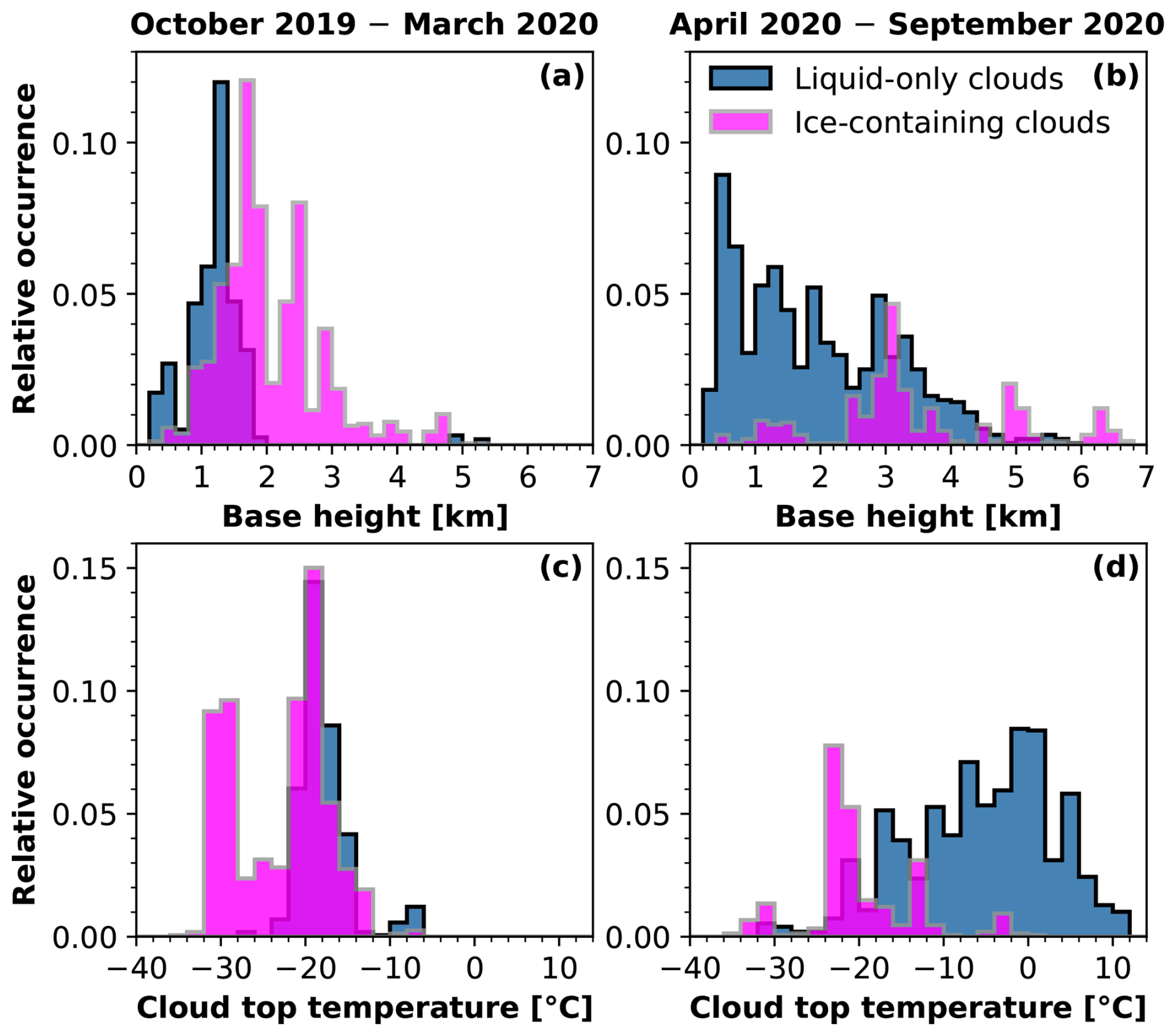
Figure 7 Histograms of liquid-dominated layer base height (a, b) and cloud top temperature (c, d) for free-tropospheric, and thus decoupled, clouds as in Jimenez et al. (2025) but separated for winter (October 2019–March 2020, panel a and c) and summer (April 2020–September 2020, panel b and d). Liquid-only clouds are in blue, and ice-containing clouds in pink.

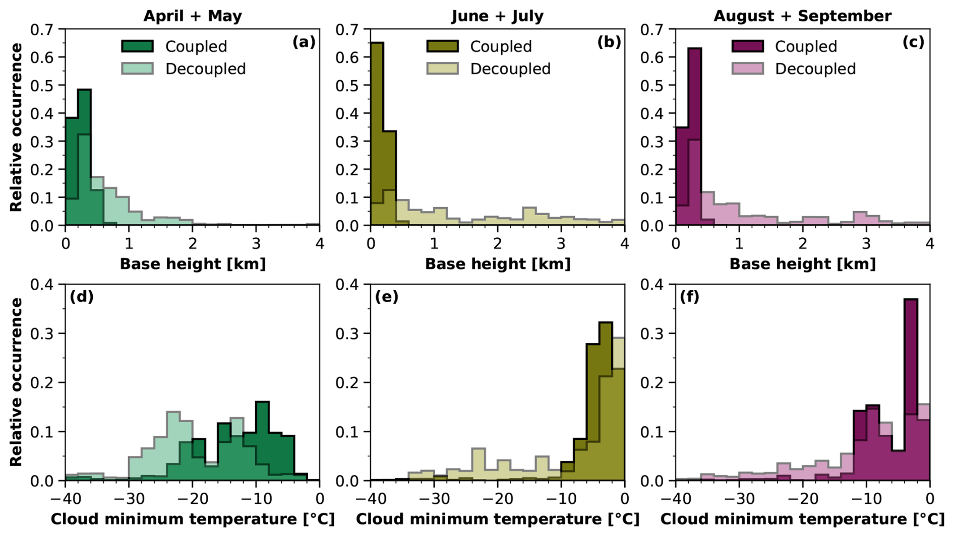
Figure 8 Histograms of liquid-dominated layer base height (a–c) and cloud minimum temperature (d–f) for April + May (a, d), June + July (b, d), and August + September (c, f). Each histogram shows the distribution for coupled (darker colors) and decoupled (brighter colors) cases.

To contrast the clouds analyzed in this study, which include clouds well below 500 m, with the findings from Jimenez et al. (2025) histograms of the cloud top temperature and the liquid-dominated base height for the coupled and decoupled clouds are shown in Fig. 8. In August + September the decoupled clouds showed a much lower liquid-dominated layer base height, compared to June + July, with a clear maximum below 500 m. The layer base height distribution for decoupled clouds in April + May is similar to the one for August + September. However, there is a strong difference in the cloud minimum temperature, with much colder temperatures in April + May, mostly below −10 °C, while the clouds in August + September were usually observed at T > −10 °C. The free-tropospheric cloud statistics indicates that the decoupled, ice-containing clouds at T > −10 °C, e.g., in August + September, are mostly likely still influenced by surface processes and a clear separation from the surface is only reached in higher altitudes.

4.3.3 Surface INP concentrations

The surface INP measurements were used to identify days with enhanced INP concentration for INPs which activate ice formation at temperatures above −15 °C. To separate between high and low concentrations the 30th percentile of INP concentration active at −15 °C was used (= 6 × 10⁻⁴ N_INP L⁻¹). Clouds which were sampled during days with high INP concentration show an increased fraction of ice-containing clouds in the temperature interval between −7.5 and −5 °C (not shown). Those clouds, which were observed during days with enhanced INP concentration, were additionally separated by their coupling state. The respective fraction of ice-containing clouds is shown in Fig. 9. SML-coupled clouds under high INP load (red) revealed an enhanced fraction of ice-containing clouds throughout the whole temperature range between −20 and −5 °C cloud minimum temperature, on average 21 % higher. The largest difference was found for clouds with a minimum temperature between −7.5 and −5 °C with 70 % of the coupled clouds were ice-containing, while only 35 % of the decoupled clouds. Clouds which were sampled during days with low INP concentrations showed lower fraction of ice-containing clouds at temperatures above −20 °C, independent of their coupling status.

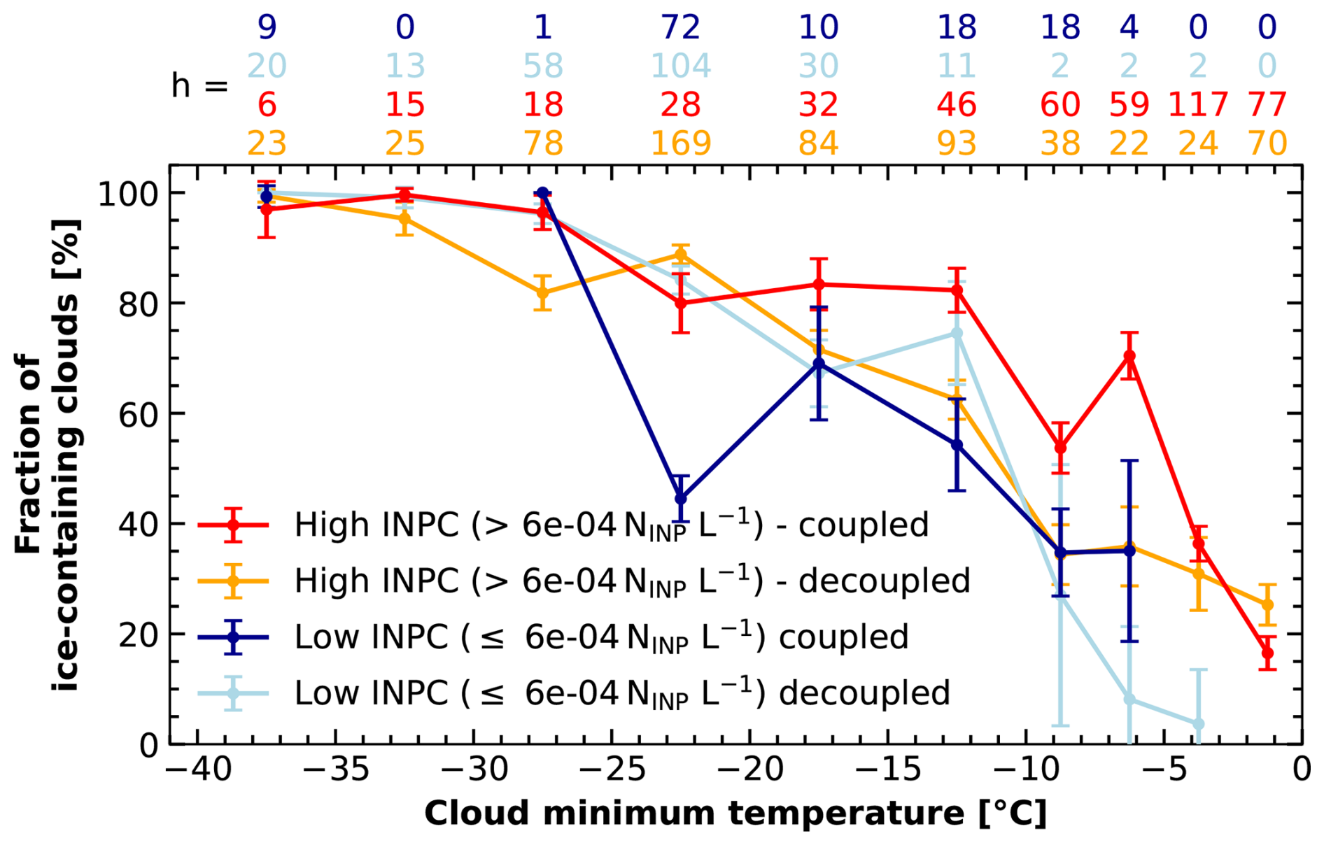
Figure 9 Same as Fig. 5 but distinguished between high (red and orange) and low (light and dark blue) INP concentrations active at T > −15 °C. The data were further separated by their coupling state. The red and dark blue shows data for surface coupled clouds and yellow and light blue for decoupled clouds.

4.3.4 Trajectory residence times

Figure 10 shows the fraction of ice-containing clouds as a function of their cloud minimum temperature during the whole MOSAiC period, represented by the blue line in both panels. In each panel, additionally, the dataset separated by different trajectory residence times is presented. In Fig. 10a the dataset was split for residence times below (red line) and above (yellow line) 15 h. This threshold was derived by a sensitivity study and was set to the time where the largest effect was found. Clouds corresponding to back-trajectories with shorter residence times to the ice edge (less or equal to 15 h) revealed an enhanced fraction of ice-containing clouds of 71 % between −7.5 and −5 °C cloud minimum temperature during 32 h of observations. The fraction of ice-containing clouds with longer residence times was 58 %. A contributor to the increased fraction of ice-containing clouds with shorter residence time could be a source of INPs close to the ice edge, e.g., in the marginal ice zone. The fraction of ice-containing clouds for residence times longer than 15 h is hardly changed compared to the whole dataset. Note that the fraction of clouds with residence times shorter than 15 h is rather small relative to the whole year of observation.

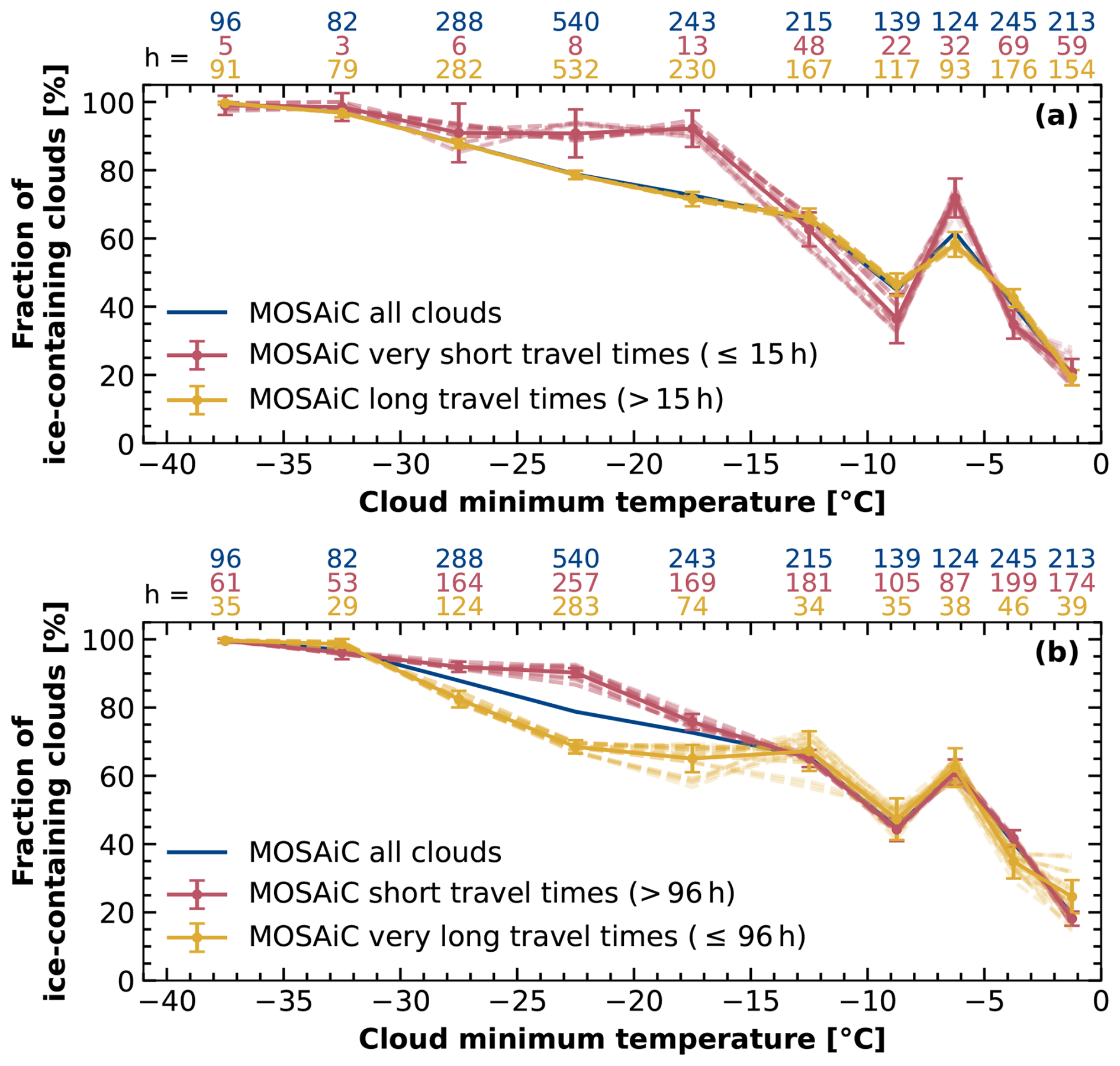
Figure 10 Same as Fig. 5 but for the whole MOSAiC period (blue line in panel a and b). Panel (a) shows additionally the respective analysis separated for residence times shorter (red) or longer (yellow) than 15 h, and panel (b) the data separated for residence times shorter (red) or longer (yellow) than 96 h. The dashed lines depict results based on single trajectories of the ensemble, the solid line shows the mean results from all trajectories.

Residence times above sea ice of more than 3–4 d lead to a reduction of ice-containing clouds at temperatures below −15 °C, as shown in Fig 10b, which contrasts the observations of clouds corresponding to times below (red) and above (yellow) 96 h. Residence times shorter than 96 h increased the fraction of ice-containing clouds between −15 °C and −30 °C by 14 % (22 % between −20 and −25 °C). This is likely due to a depletion of long-range transported INPs, for example, via the sedimentation of a formed ice crystal. The distribution of ice-containing clouds above −15 °C, however, does not change for residence time below and above 96 h.

4.4 EDR analysis

EDR were used to investigate the influence of turbulence and thus SIP on ice occurrence. The EDR were analyzed following Chellini and Kneifel (2024). For each time step EDR in log-scale from the uppermost 500 m of the cloud were averaged. In case of a cloud top height below 500 m or a shallower cloud, the EDR of the whole cloud column until cloud top was analyzed. The threshold used here to separate between high and low EDR cases differed slightly from those used in Chellini and Kneifel (2024), since the EDR values of the clouds analyzed in this manuscript were mostly below 10⁻³ m² s⁻³ (upper threshold in Chellini and Kneifel, 2024). We used the 90th (log₁₀(EDR) > −3.57) and the 50th (log₁₀(EDR) < −4.4) percentile of all mean EDR, to separate the EDR states. Yet, no influence of the EDR on the fraction of ice-containing clouds has been found (see Fig. A3).

Table 3 Mean log₁₀(EDR) of the uppermost 500 m (or subsection thereof in case of shallower clouds) of the clouds with cloud minimum temperature between −7.5 and −5 °C for each 2-months period analyzed in Fig.6, separated by their coupling state and phase. The EDR were calculated in m² s⁻³.

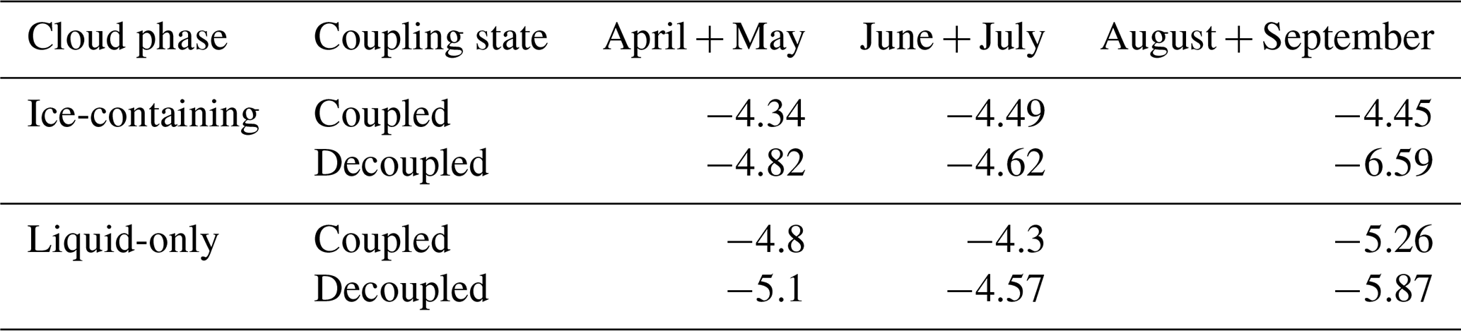
The mean EDR values for coupled and decoupled clouds with temperatures between −7.5 and −5 °C in April + May, June + July, and August + September contrasted for the different cloud phases are presented in Table 3. In general, the values are higher in case of a coupled cloud. However, in terms of cloud phase no clear picture was found. The highest EDR values were found in coupled liquid-only clouds in June + July (log₁₀(EDR) = −4.3). The lowest EDR values were found for decoupled ice-containing clouds in August + September (log₁₀(EDR) = −6.59).

5 Discussion

The presented analysis reveals a strong influence of the SML-coupling on the probability of clouds observed between April and September with a minimum temperature above −15 °C to contain ice. From the numbers annotated above Fig. 5 it is clear that few cloud observations with cloud minimum temperature below −15 °C contributed to the statistics for June + July and August + September. This is due to the fact that only the lowest liquid-containing cloud layer was analyzed. In case of multiple liquid-containing cloud layers, as it was regularly observed during MOSAiC (Silber and Shupe, 2022), the upper cloud was not included, as the lidar was already attenuated by the lower layer. This prevented the identification multiple liquid-dominated layers, which were, however, not the focus of this study. Also, no pure ice clouds were considered, as only clouds with a liquid-dominated layer were incorporated in the analysis. Another limiting factor was the relatively warm surface temperatures in July and August, often above 0 °C (see Fig. 2a), that caused many liquid-precipitating clouds. These clouds were removed from the analysis, as they would likely be miss-identified as pure liquid clouds by the analysis. Blowing snow was considered by removing periods with increased surface wind speed of higher than 15 m s⁻¹. Finally, all clouds that indicated potential seeder-feeder situations as described for example by Ohneiser et al. (2025), i.e., all clouds with a second cloud within 1 km above, were also removed from the dataset.

The observed results of a higher fraction of ice-containing clouds under SML-coupled situations at temperatures above −15 °C from April until September is a strong indicator for the impact of locally produced INPs on the cloud properties. INPs that initiate ice formation at such warm temperatures usually contain biogenic material (Pereira Freitas et al., 2023; Hartmann et al., 2025), which may come from the marginal ice zone, melt ponds, or polynyas (Irish et al., 2017; Wilson et al., 2015; Hartmann et al., 2020, 2021; Mavis et al., 2025). Creamean et al. (2022) and Barry et al. (2025) reported a maximum of INPs active above −15 °C observed during MOSAiC between May and September at the surface. Under coupled situations these INPs likely got mixed into the low-level clouds and hence increased the ice occurrence in these clouds. This is supported by the strong influence of the coupling analysis on the fraction of ice-containing clouds on days where a high INP load active above −15 °C was sampled on the ground (and thus within the boundary layer). A combined temporal and coupling state (as in Fig. 6) and INP-based analysis of the dataset was not possible. The data coverage would have been too sparse and the resulting uncertainty would dominate any finding. Additionally, a back-trajectory residence time above sea ice analysis revealed a decreased fraction of ice-containing clouds a temperatures below −15 °C after 3–4 d. This can be caused, for example, by a depletion of INPs below −15 °C with time.

In August + September the decoupled clouds also showed a high fraction of ice-containing clouds. The applied coupling analysis only considers the state of the cloud at the time of observation. However, clouds which were identified as decoupled above Polarstern may have been coupled to the surface before. Also a weak exchange with the SML, not covered by the coupling approach, can introduce alternations of the cloud properties. The weak stability in fall during MOSAiC (Jozef et al., 2024), e.g., can support a mixing of locally produced INPs with biogenic material into the free troposphere, which would increase the availability of INPs active above −15 °C. Contrasting the results of the boundary layer clouds presented in this manuscript with the free-tropospheric ones analyzed in Jimenez et al. (2025), it was shown that the decoupled clouds in August + September were often observed at rather low altitudes and warm subzero temperatures, which increased the likelihood of a surface influence on these clouds (see Fig. 8). Yet, increased long-range transport can also fill the respective INP reservoir in the free-troposphere. Even though Polarstern was located far in the north and even crossed the North Pole during August + September the probed air masses were associated with rather short residence times to the measurement site, often less than 4 d (Fig. 2).

The applied lidar is less sensitive to ice detection as, for example, a cloud radar. The lidar was utilized due to its lower detection limit and the focus of this study, which are low-level clouds. However, the same analysis as presented in Sect. 4.3.1 and 4.3.2 was done using a cloud radar based cloud-phase separation approach. The Cloudnet target classification data was used to identify ice-containing clouds. The results for all clouds in each 2-month periods for the whole MOSAiC year is shown in Fig. A2. The results of the coupling-separated periods between April and September are shown in Fig. 11. The higher sensitivity of the cloud radar to identify ice is striking. More ice-containing clouds were identified throughout all temperature intervals and under all coupling situations. However, especially at temperatures above −10 °C, more hours of cloud observations were analyzed using the lidar approach, proving the necessity of its application. Overall, the radar-based coupling analysis reveals the same pattern of more ice-containing clouds under surface coupled conditions, especially at temperatures above −10 °C, in all 2-months periods.

Figure 11 Same as Fig. 6 but using the cloud radar for phase separation.

6 Conclusions

In this study, the first annual cycle of heterogeneous ice-formation temperatures for Arctic mixed-phase clouds is presented for clouds observed during the MOSAiC year from 2019 to 2020, with a special focus on low-level clouds. It was shown that no cloud with minimum temperatures above −10 °C was observed from October to end of March. From April to September, a maximum of ice-containing clouds was found between −7.5 and −5 °C. This finding indicates an influence of biogenic material containing INPs, which are needed for ice formation at these temperatures. The presented results corroborate the findings from Creamean et al. (2025) and Barry et al. (2025) who observed a peak in the INP number concentration during MOSAiC during summer.

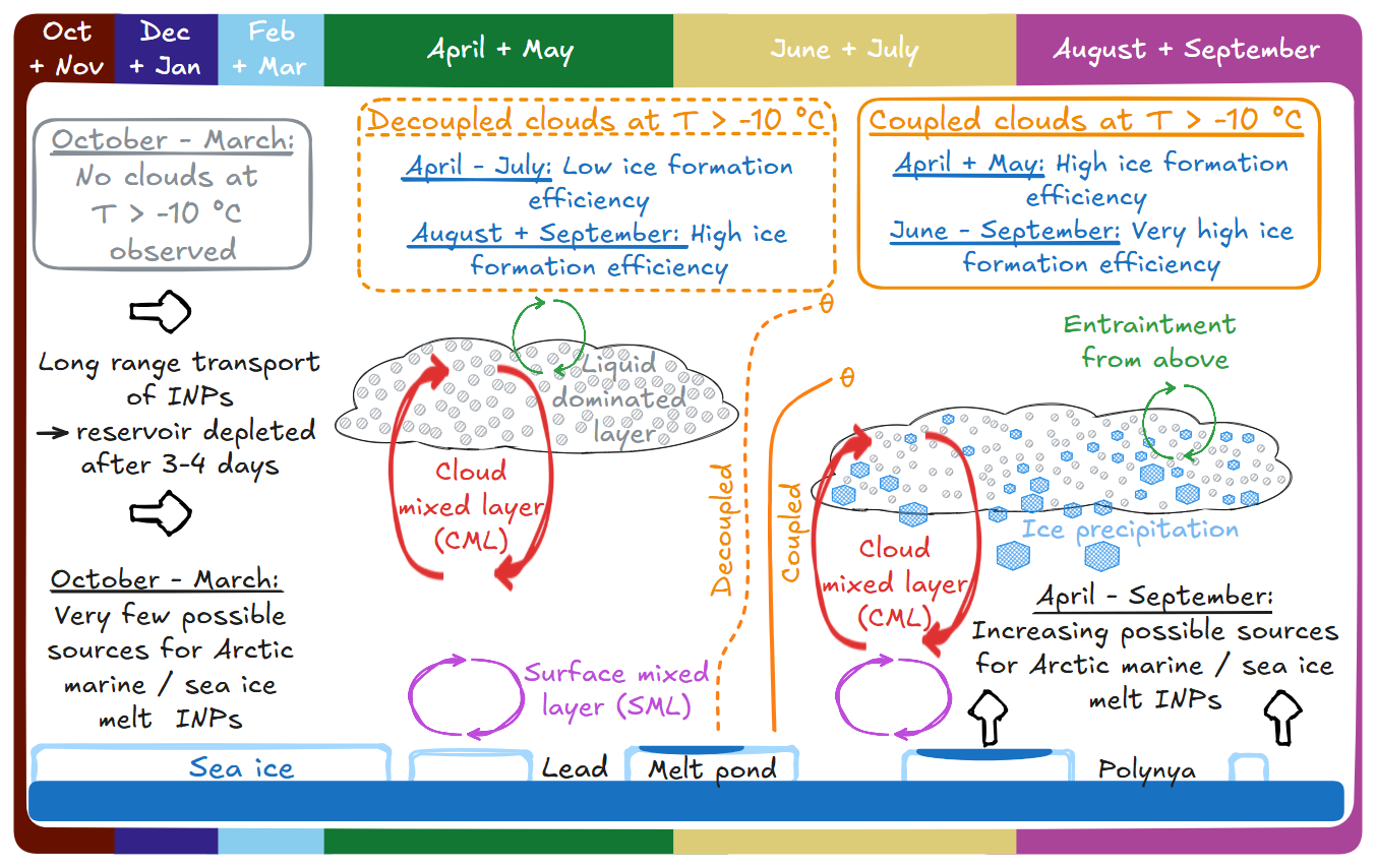
Figure 12 Idealized summary of the observed mechanisms driving heterogeneous ice formation in Arctic low-level mixed-phase clouds at T > −10 °C during the MOSAiC expedition. The curved arrows indicate different relevant mixing mechanisms: entrainment from above (green), cloud mixing (red) and surface mixing (pink). Black arrows show potential pathways of INP supply in the boundary layer and free troposphere (long-range transport and local marine and sea ice melt emissions). In orange two example potential temperature (Θ) profiles are shown, one for a coupled state (solid line) and one for a decoupled state (dashed line).

The most relevant processes identified in this study for low-level clouds to form ice at temperatures above −10 °C are summarized in Fig. 12. From October to March no clouds were observed above −10 °C. Due to a sea-ice fraction of close to 100 %, absent melt ponds, and a very low lead fraction from late autumn to early spring, very few local sources of INPs can be expected during this time. However, this may change due to the changing Arctic, where the warming is most prominent in winter. From April to September, the dataset was separated by the cloud SML coupling state. The coupling of the cloud mixed layer (CML) to the surface mixed-layer (SML) was derived using the potential temperature profile from radiosonde measurements. A strong influence of the coupling state on the likelihood of clouds to contain ice at high ice-formation temperatures was found from April to July. Coupled clouds showed a 2–3 higher probability to contain ice at T > −15 °C when the cloud was coupled to the SML in these months (up to 60 % fraction of ice-containing clouds). In August + September, the ratio of the fraction of coupled to decoupled ice-containing clouds decreased to 1.3 (85 % vs 65 % fraction of ice-containing clouds, respectively). Similarly, from April to July, clouds were more frequently observed as coupled at T > −15 °C, while in August + September, the clouds were more often identified as decoupled. The increased ice formation under SML-coupled situations was attributed to an increased availability of INPs that contained biogenic material in the SML, likely from local Arctic marine sources, such as the marginal ice zone. From April to September, the fraction of possible sources for such marine and sea ice melt INPs increased due to an increase in the lead and melt pond fraction and a decrease in sea-ice fraction with time. Barry et al. (2025) proved by means of heat treatments, that the INPs measured during the MOSAiC summer at the surface were almost entirely biological ones. The INPs can be mixed into the cloud if the CML, which is driven by convection from radiative cloud top cooling, reaches the SML.

It is likely that the decoupled clouds in August + September were still to a significant part influenced by surface processes. Weaker stability during fall may result in an increased exchange between the PBL and the free troposphere and hence a stronger transport of INPs from the surface to the free troposphere. The derived liquid-dominated layer heights were lower in August + September (mostly below 500 m) compared to June + July, resulting in more detected decoupled clouds in August + September. Additionally, the minimum temperature for the decoupled clouds in August + September was rather high (mostly above −10 °C) and hence ice-formation at relatively warm subzero temperatures was likely to be observed. Yet, an increased long-range transport of INP-carrying air masses could also be the cause of the observed phenomenon. For example, Ansmann et al. (2023) showed that the free tropospheric INP load at 2000 m during the MOSAiC expedition was dominated by continental particles throughout the year.

Heterogeneous ice-formation temperatures were linked to the INP load at the surface, using filter samples collected during MOSAiC and the coupling analysis. During days where the INP concentration active above −15 °C was above its 30th percentile (6 × 10⁻⁴ N_INP L⁻¹), the probability of SML-coupled clouds to contain ice at temperatures between −20 and −5 °C increased by more than 20 %. Between −7.5 and −5 °C, for example, the fraction of ice-containing SML-coupled clouds during days with a high INP load active above −15 °C was 70 %, while it was 35 % for decoupled clouds. Finally, residence times of trajectories initiated at the liquid-dominated layer base height were used to show that shorter times (< 15 h) correspond to an increase in the fraction of ice-containing clouds for −7.5 °C > T > −5 °C. Residence times of more than 96 h correspond to a decrease in the fraction of ice-containing clouds below −15 °C, indicating a depletion of INPs after 3–4 d. No difference between longer or shorter residence times of 96 h was observed for clouds with T > −15 °C. These findings support the hypothesis that locally produced INPs are a major driver of the enhanced ice occurrence at low-supercooling temperatures, while long-range transported INPs are dominating the ice-production below −15 °C.

The presented feature of increased ice formation at relatively warm subzero temperatures under SML-coupled situations in Arctic low-level mixed-phase clouds should be further analyzed, with a focus on contrasting Arctic and Antarctic cloud properties, given the recent changes also happening in Antarctica. Also, the development of the seasonal cycle should be investigated further. Under the changing conditions in the Arctic, clouds at warm subzero temperatures might be observed soon also in Arctic winter (Jenkins et al., 2024). Additionally, the availability of sources may change under a warming Arctic. Even though a clear associative connection between surface-based measurements of INP concentrations and cloud ice-microphysics was established here, not all mechanisms at play could yet be quantified. Modeling results as well as observational datasets from field campaigns but also long-term records from land-based stations should be harvested to investigate this phenomenon in more detail. Finally, if sources at the surface play a significant role in the cloud microphysical properties, this should reflect on the radiative properties of the cloud. Hence, it is worth investigating whether clouds coupled to the SML have a different cloud radiative effect. In this regard, the new satellite mission EarthCARE (Wehr et al., 2023) provides valuable opportunities.

Appendix A: Volume depolarization threshold for ice detection

To derive a lidar volume depolarization threshold for ice detection, a dependency of the IWC and the volume depolarization was derived. The extinction coefficient α was calculated using the IWC-Z-T and the α-Z-T relationships from Hogan et al. (2006) with Z as cloud radar reflectivity and T as temperature. The extinction coefficient was converted to particle backscatter coefficient by applying a lidar ratio of 30 sr (Ansmann et al., 1992). Finally, from the particle backscatter coefficient, a molecular extinction coefficient derived following Elterman (1968) and Teillet (1990), a molecular lidar ratio of $\frac{\mathrm{8}\mathit{\pi }}{\mathrm{3}}$, and an approximated molecular volume depolarization ratio of 0.01 (Biele et al., 2000), the volume depolarization ratio was calculated based on Freudenthaler et al. (2009). In Fig. A1 the results are shown for T = −5 °C and T = −30 °C. From this relationship it was concluded that a distinct ice identification is only possible at a volume depolarization value above 0.03 (indicated by the dashed purple line). At T = −5 °C this depolarization value corresponds to an IWC = 8 × 10⁻⁵ kg m⁻³ (blue vertical dashed line) and at T = −30 °C to an IWC = 4 × 10⁻⁵ kg m⁻³ (orange vertical dashed line). Additionally, the IWC threshold of 10⁻⁶ kg m⁻³ from Bühl et al. (2013) is indicated by the vertical red line.

Figure A1 Theoretical derived volume depolarization – IWC dependency.

Figure A2 Same as Fig. 5 but using the cloud radar for phase separation.

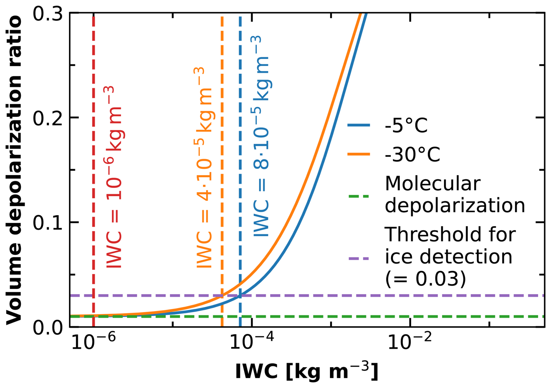
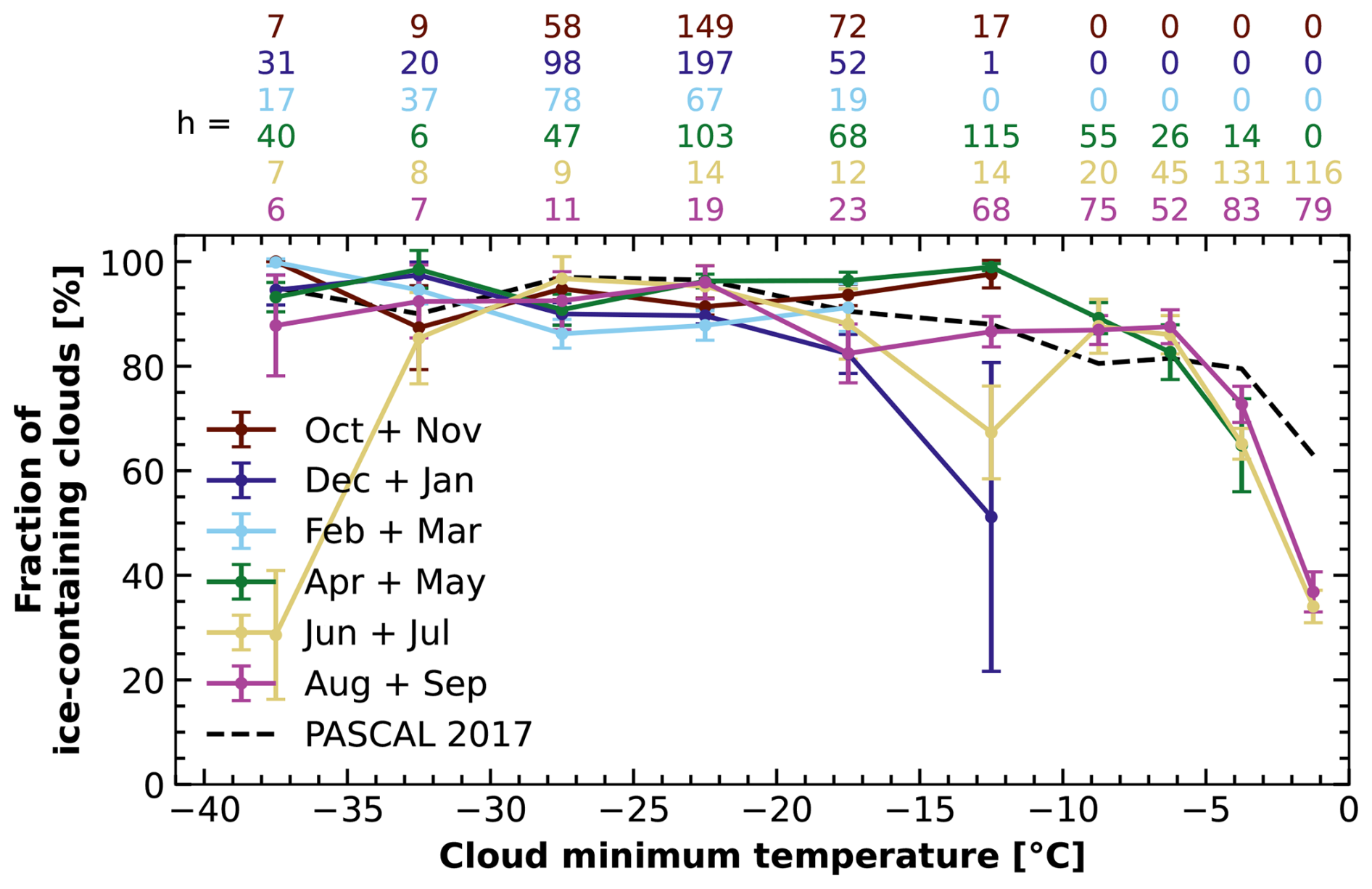
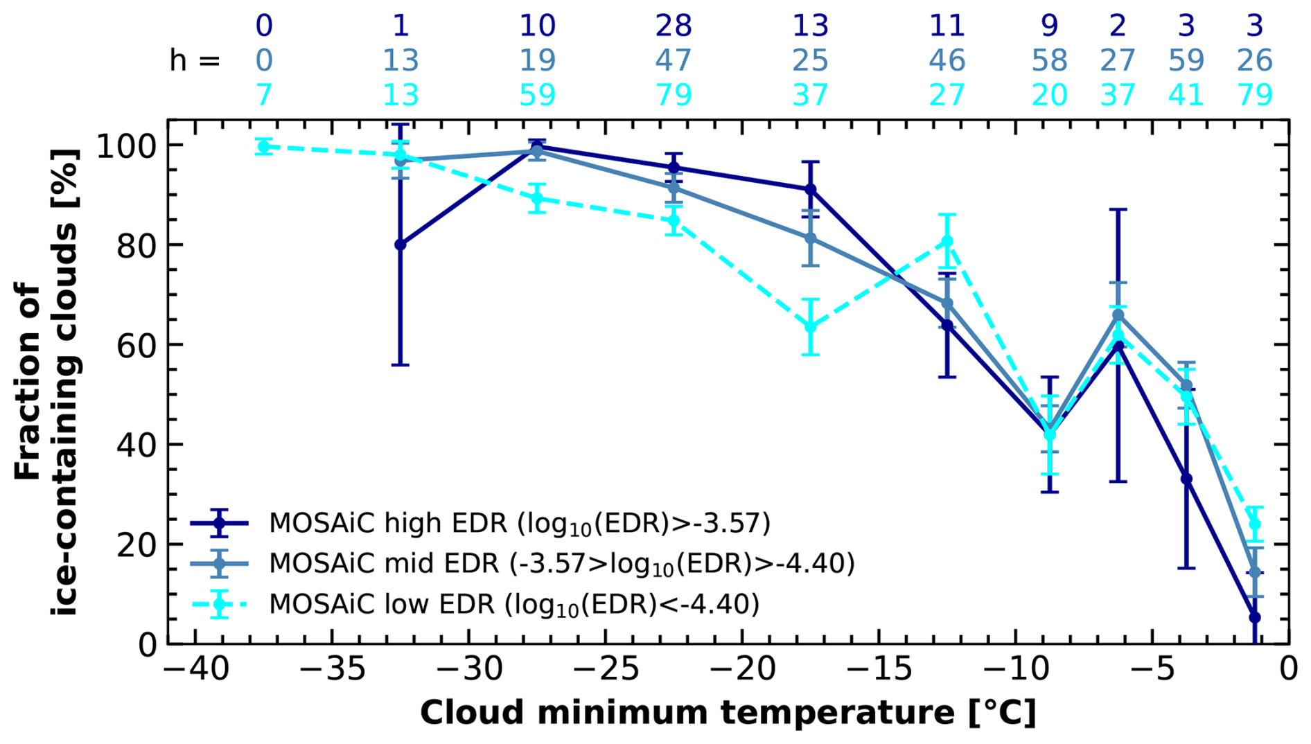
Figure A3 Fraction of ice-containing clouds as a function of their minimum temperature during the MOSAiC expedition, separated for the mean EDR observed in the upper 500 m of the cloud.