Measurement report: Temporal variability of vertical profiles of CO₂ and CH₄ over an urban environment

Improving estimates of city emissions requires a better understanding of pollutant transport dynamics within the urban boundary layer (UBL), particularly for greenhouse gases (GHGs), given the importance of cities in mitigation efforts. Due to heterogeneous emission sources and complex atmospheric processes, diverse observational datasets are needed to constrain urban transport and support inversion frameworks to estimate emissions. In this context, vertical profiles of GHGs provide critical information. This study presents results of 11 vertical profiling campaigns conducted in Krakow, southern Poland, over one year (March 2021–February 2022). The aim was to obtain high-resolution measurements of CO₂ and CH₄ mole fractions, together with key meteorological variables, within the urban boundary layer of a mid-latitude city with a population of close to one million. Such datasets of vertical profiles up to 280 m above ground level (a.g.l.) are rare, particularly within city limits, and are intended to support the development of a city-scale inversion system. Measurements were carried out using a Picarro G2311-f cavity ring-down spectrometer deployed on two platforms: (i) a tethered tourist balloon in the city centre, reaching up to 280 m a.g.l., and (ii) an uncrewed aerial vehicle (UAV) operating up to 100 m a.g.l. For UAV measurements, the analyser remained on the ground and sampled air through a 200 m tube. To our knowledge, this is the first application of this approach for vertical GHG profiling. Meteorological variables, including temperature, relative humidity, pressure, and wind, were measured using calibrated low-cost sensors mounted on both platforms. The observations enabled a detailed analysis of the structure and evolution of the UBL under varying meteorological conditions throughout the year. The altitude range of the platforms allowed frequent detection of stable nocturnal boundary layers, as well as elevated CO₂ and CH₄ plumes above them during the night and morning periods, likely associated with strong emission sources outside the city. In general, the dataset provides a valuable record of high-resolution vertical GHG distributions and meteorological conditions in an urban environment. It helps fill a key observational gap in the lower troposphere over cities and offers important insights for studying urban boundary layer processes and improving emission estimates.

1 Introduction

Stabilising the global temperature rise in the 21st century below 2 °C requires comprehensive mitigation efforts targeting emissions of all greenhouse gases (GHGs), including both CO₂ and non-CO₂ GHGs (Ou et al., 2021; IPCC, 2023). Despite several global policies already implemented (most notably the 2015 Paris Agreement; UN, 2015), the mole fractions of the main atmospheric greenhouse gases emitted through human activity have continued to maintain their historically high growth rates. The global average CO₂ dry air mole fraction rose by 2.13 ppm (1 ppm = 1 µmol mol⁻¹), reaching 417.06 ppm in 2022 (NOAA, 2024), and is now over 50 % higher than the pre-industrial level of approximately 280 ppm. Background levels of atmospheric methane in 2022 have also increased to an average of 1911.9 ppb, with an annual increase of 14.0 ppb yr⁻¹, the fourth largest annual increase recorded since NOAA's systematic measurements began in 1983. The growth rates of both primary greenhouse gases have remained high over more than a decade, raising concern about the realism of planned mitigation measures. A recent report from United Nations Environment Programme (United Nations Environment Programme, 2025) estimated that the current global warming projections foresee a total global warming projection of between 2.3 and 2.5 °C by year 2100 – assuming that all declared Nationally Determined Contributions are fully implemented. If only the policies already in place (as of 2025) are considered, the projected global average temperature is 2.8 °C, underlining the urgency of further mitigation efforts.

Urban areas, which constitute 2 % of the land surface, are responsible for around 70 % of fossil-fuel CO₂ emissions (IEA, 2008; Seto et al., 2014), which makes them particularly relevant in the context of emission mitigation. However, due to cultural, political and administrative differences, combined with the extreme administrative, technical and financial complexity of implementation of city-wide policies targeting GHG emissions, the development of mitigation strategies for cities has been fragmented and focused on the largest and usually wealthiest, urban agglomerations. One of the greatest challenges in developing such policies results from the high spatial and temporal heterogeneity of urban GHG emissions. Dispersed sources with variable diurnal or seasonal variability, like road transport and individual heating, often contribute to the overall emission budget (Duren and Miller, 2012), making the accurate quantification of emissions through bottom-up approaches challenging. In response, various top-down techniques for city emission monitoring have been developed. Direct estimations of city emissions using observations have been performed using in situ ground-based atmospheric observations (Lowry et al., 2001), airborne measurements using mass-balance technique (Mays et al., 2009; Turnbull et al., 2011; Cambaliza et al., 2014; Heimburger et al., 2017; Ashworth et al., 2020; Klausner et al., 2020), and more recently using remote sensing total column observations, either from ground based instruments (Dietrich et al., 2021; Park et al., 2024) or from space-borne sensors (e.g. de Foy et al., 2023). Each of these approaches, however, has important limitations for monitoring urban emissions, including incomplete representation of the full atmosphere (surface-based), high measurement costs (airborne), and low sensitivity to weaker sources (remote sensing). More importantly, each direct emission estimation method heavily relies on assumptions regarding atmospheric flows in urban areas, for which additional observation datasets are valuable for more accurate wind fields, or for validation.

To overcome challenges in direct emission estimations, the modelling frameworks based on Bayesian inversions have gained prominence, as they allow to representation of complex atmospheric conditions, and to utilize limited observations to the maximum effect in a strict methodological framework. Inversion systems were first developed for global (Enting et al., 1995; Rödenbeck et al., 2003) and regional scales (e.g. Gerbig et al., 2003; Bergamaschi et al., 2015), but as the resolution of the models and their overall accuracy improved, city-scale inversions became feasible. One of the earliest attempts for application at the city-scale was reported by Lauvaux et al. (2013), and was followed by a series of studies in other cities (e.g. Lauvaux et al., 2016; Nalini et al., 2022; Chen et al., 2022; Ponomarev et al., 2026). Nowadays, inversion modelling is considered to be one of the recommended techniques in the World Meteorological Organisation's report on Urban Emission Observation and Monitoring Good Research Practice Guidelines (WMO, 2025). In those modelling systems, one of the primary challenges is the existence of the transport model error, difficult to estimate and in most cases non-random. As accuracy of inferred emissions critically depends on the transport model's ability to correctly simulate the pollutant's dispersion, selection of appropriate model and fine-tuning of its settings are necessary steps for realistic emission estimates. Despite gradual development of the models at the city scales, often spurred by activities within larger multi-partner projects like INFLUX (Lauvaux et al., 2016) or ICOS-Cities (ICOS-Cities, 2026), no standard solutions exist for high-resolution urban settings, and additional observations over various urban landscapes are necessary for setting up a modelling system for any new city.

High-resolution information in the vertical profiles inside the cities is one of the most valuable data streams for modelling-based studies, as it provides information about processes, and at scales, most relevant to the transport model errors. Direct profile observations of meteorological data can be used to assess the model configuration and determine the accuracy of key variables influencing pollutant dispersion, including temperature, wind speed and direction, and the height of the urban boundary layer (UBL). Measurements of the lowest part of the troposphere are especially important. While meteorology within the city is driven by mesoscale weather systems (Zhang et al., 2022), special phenomena occur (city canyons, urban heat island) that modify the atmospheric characteristics and GHG transport. Highly heterogeneous urban landscapes drive the atmosphere in the city, and any modelling system must realistically represent them. Simultaneously, emissions of GHGs occur on the same characteristic spatial scales, as many emissions are also tightly linked to land-cover (e.g. transport for CO₂, waste/sewage for CH₄) (Li et al., 2014; Giovannini et al., 2020; van der Woude et al., 2023). This implies that, for urban applications, models should ideally be capable of resolving transport at spatial resolutions of 100 m or finer, within the lower end of the so-called “grey zone”, where turbulence is only partially resolved (Honnert et al., 2020). In practice, it has been shown that city-scale simulations of the GHGs can be run at coarser (1 km) resolutions using urban parametrisations of boundary layer processes developed for regional applications, provided that the transport error is carefully assessed (e.g. Lopez-Coto et al., 2020b, a; Peng et al., 2023). While inverse frameworks using surface-data only, heavily supported by ceilometers and LiDAR for detection of the mixed layer have been employed (Lopez-Coto et al., 2020a), data from the atmospheric column can be of high benefit as sources located in the vicinity of measurement points might not yet be fully mixed across the UBL, potentially leading to biased estimations. Measurements in the lowest part of the troposphere also open the possibility of utilisation of the night-time data, discarded in most inverse modelling applications by providing an accurate representation of the vertical structure within the stable boundary layer (SBL) together with transition between stable and convective BL (CBL) (Lopez-Coto et al., 2020a). The ability to simultaneously measure vertical variability of meteorological variables and GHG profiles could then serve a double purpose – by helping to correctly fine-tune the modelling framework, as well as to provide data used for the inversion.

Research on the vertical structure of GHGs in urban areas can be attempted using in situ tall-tower infrastructure (Lowry et al., 2001; Richardson et al., 2017), aircraft (Fiehn et al., 2020; Gałkowski et al., 2021), uncrewed aerial vehicles (UAVs; Kunz et al., 2018) or tethered balloons (Li et al., 2014). Airborne platforms are typically the best choice for this purpose, as only they allow measurements throughout the boundary layer. The atmospheric mole fractions of GHGs on airborne platforms can be performed by in situ sensors (e.g. Kunz et al., 2018; Turnbull et al., 2011), by discrete sampling (Lampert et al., 2020), and using aircore systems (Andersen et al., 2018). Remote sensing instrumentation can also be used for this purpose, but studies published so far have mostly targeted point sources rather than cities (e.g. Krings et al., 2018; Wolff et al., 2021). Especially over the densest parts of the cities, obtaining such data poses an organisational and logistical challenge, as measurements of vertical profiles require airborne platforms equipped with heavy instrumentation to achieve the necessary precision and accuracy. In addition, many cities limit the possibility to fly low over their central areas due to safety and security considerations. Consequently, the amount of urban vertical profile data is still relatively limited, and most studies utilising airborne sampling throughout the BL either limit measurements to the areas outside of the urban zones, especially if the mass-balance technique is attempted (Turnbull et al., 2011; Fiehn et al., 2020)

In this work, we report measurements of vertical distributions of basic meteorological variables (temperature, humidity, wind) and selected GHGs (CO₂, CH₄) within the urban boundary layer of Krakow, a city of approximately 800 000 inhabitants, collected over 11 single-day measurement campaigns throughout 2022. We used two dedicated airborne platforms: (i) a tethered tourist balloon operating in the strict city centre as the primary platform, allowing for in situ measurements of up to 280 m a.g.l., and a UAV platform flying to the altitude of 100 m a.g.l. Both platforms used the same instrumental setup, including a precise weather station and a wavelength-scanning cavity ring-down spectrometer (CRDS) Picarro G2311-f, carried onboard (balloon) or connected to the airborne platform by a long tube (UAV). All reported measurements are directly linked to the appropriate WMO reference scales through calibration against standard reference gas mixtures. To the best of our knowledge, this is the first work reporting measurements by UAV connected to a high-precision instrument through a long tube for precise vertical profile measurements. Although Andersen et al. (2018) already showed an example of how this can be achieved when the Aircore system is employed with UAV, with additional advantage of allowing for free flight path, unconstrained by the tube presence. However, their system exhibits greater spatial smoothing – caused by mixing within the Aircore tubing – and is more complex in terms of design, manufacturing, and data analysis. In studies in which dedicated on-board sensors were employed, lower measurement accuracy is usually achieved and more effort is needed to assure the link to the WMO reference scales (e.g. Zhou et al., 2025; Bolek et al., 2024).

We analyse the measurement data to discuss diurnal and seasonal variability of the GHGs in the lower troposphere over Krakow, with particular emphasis of boundary layer dynamics. We also present selected case studies for which a typical vertical structures were observed, likely linked to point source activity in the upwind areas. The presented measurements form the primary observational dataset for setup and validation of the inversion modelling framework for Krakow established as part of the CoCO2 (Prototype System for a Copernicus CO₂ service) project (ECMWF, 2026).

2 Methods

2.1 Study area

Krakow is the second largest city in Poland, located in the Lesser Poland region, with an area of 326.8 km² and the number of inhabitants reaching over 800 000 according to official statistics (USK, 2023). The Krakow agglomeration includes the city itself as well as the densely populated surrounding towns and villages, forming a metropolitan area with a total population of nearly 1.4 million. The central part of the city is located in the Wisła (Vistula) River valley, at a mean altitude of about 200 m above sea level (a.s.l.; Fig. 1). The valley is oriented along the east-west direction and surrounded by hilly terrain: in the the south by Western Carpathians foothills, relatively flat upland areas from the north (Lesser Poland Uplands region) and scattered hilly ridges closing the valley from the west. The hilltops in the immediate vicinity of the city reach over 100 m above the river valley floor, and their elevation gradually increases to the south and to the north. Overall, the surrounding topography forms a semi-concave landform open only to the east, partially sheltering the lower atmosphere above the city from the overhead winds, usually westerly. A narrow opening immediately to the west (the Krakow Gate) creates a passage through which the air can be channelled under favourable wind conditions. Multiple local scale processes are impacted by orography: it induces frequent air temperature inversions in winter, promotes cold air pool formation with katabatic flows towards the river and reduces wind speeds in the valley floor as compared to areas over surrounding hills (Sekuła et al., 2021b, a). All these factors favour the accumulation of pollutants emitted within the city in the lower boundary layer.

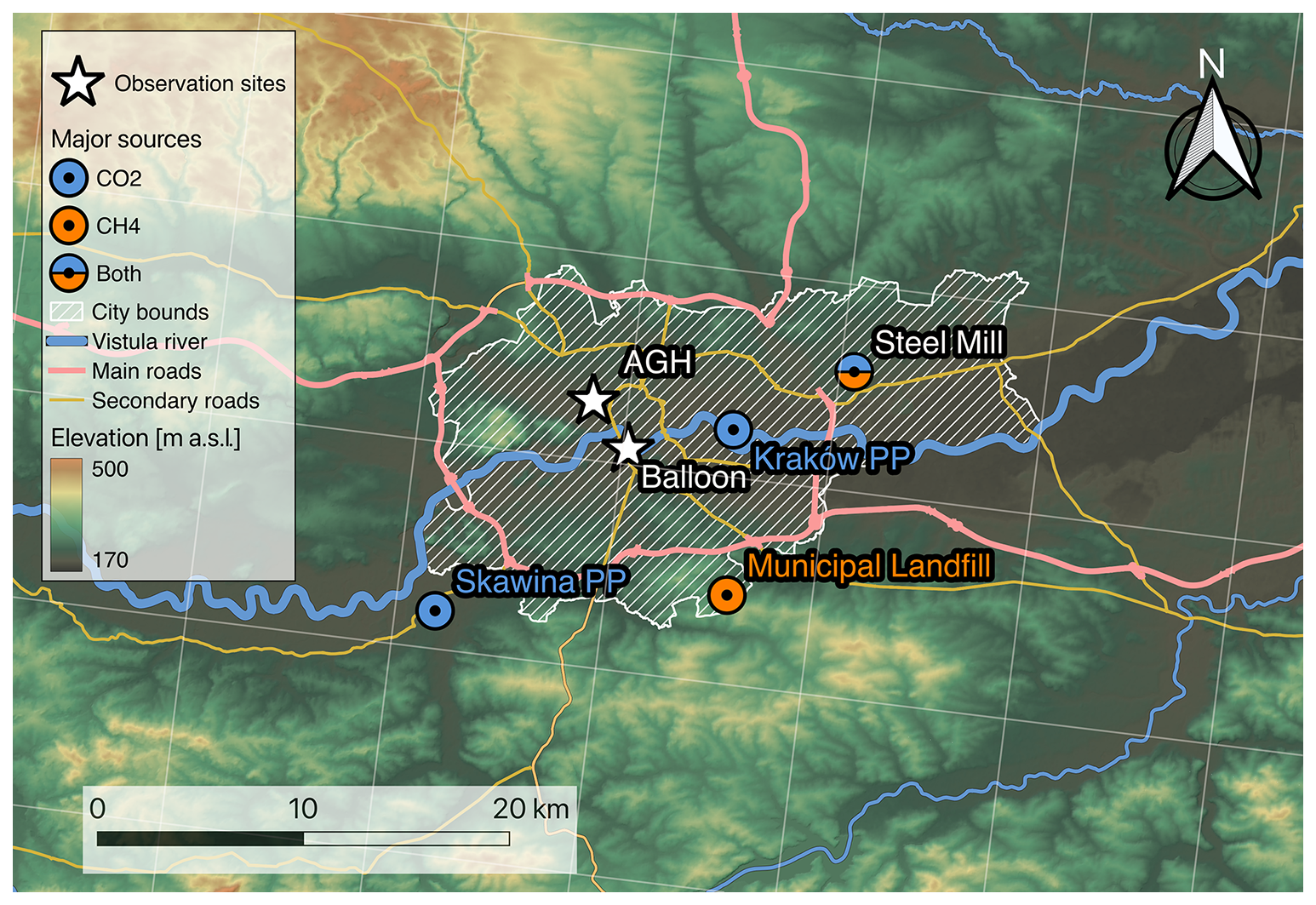
Figure 1 Study area with points of interest overlaid on a topography map. PP – power plants (coal powered cogeneration plants).

Krakow's GHG emissions are representative of a typical urban environment, with CO₂ driven by a mixture of anthropogenic and natural sources and sinks, including households, industry, transport, water reservoirs and city biosphere. Here, we understand the biosphere to consist of flora and fauna, the latter of which includes citizens and domesticated animals (Jasek-Kamińska et al., 2020). Apart from distributed emissions, three major point sources are active within the city or in its immediate vicinity: the Krakow Power Plant (PP; coal-powered, co-generation plant), a steel mill located in an industrial compound, on the eastern side of the city (Steel Mill Krakow, ArcelorMittal Poland) and the Skawina Power Plant (Skawina PP), located 15 km to the south-west of the Krakow centre (Fig. 1). A majority of CO₂ emissions from these sources are released from tall stacks. Krakow PP uses two main stacks, a primary of 120 m and an auxiliary, used in winter, of 260 m. The tall stack in Skawina is 120 m, and the steel mill in Krakow emits primarily into two 200 m stacks.

Anthropogenic emissions of CH₄ are primarily associated with the natural gas distribution network, especially dense in the urban centre, with heterogeneous and difficult to estimate leak rates. These are exacerbated by emissions from the wastewater network, limited industrial emissions (steel mill) and individual waste bins (Zimnoch et al., 2019; Menoud et al., 2021). Additionally. on the south-eastern city outskirts, a small municipal landfill (Barycz) is located, with no methane emissions reported in the Industrial Emission Database (Fig. 1; EEA, 2023).

Vertical profile sampling of GHG mole fractions and meteorological variables was carried out using two distinct measurement platforms operated at one of the two locations within the city: (i) a tethered tourist balloon operating commercially near the historical city centre (Balloon, 50.046° N 19.936° E), ca. 1800 m south from the main market square in the Old Town or (ii) a ZFS-HEXA multi-rotor UAV platform launched from the immediate vicinity of the building of the Faculty of Physics and Applied Computer Science, within the campus of the AGH University of Krakow (AGH, 50.067° N 19.913° E, Fig. 1), 2.9 km to the north-west from the balloon site. The balloon site is located among recreational areas, 30 m from the west bank of the Vistula River, with the surrounding area made up of promenades and green areas to the north and the south, and a busy communication artery passing 130 m to the west. Within the radius of one kilometre, only buildings connected to the municipal heating network were identified, i.e. those without individual combustion sources. The UAV measurements were carried out at the AGH site due to the lack of necessary infrastructure at the balloon site. Near AGH site, the surrounding area is more densely populated, mainly surrounded by university or private residential buildings connected to the central municipal heating system. A large sports stadium and a major city park are located immediately to the to the south and south-east, respectively, and a busy road passes 100 m to the north. Overall, both sites are located well within the city centre and no significant differences in the characteristics of the boundary layer are expected.

2.2 Measurement techniques

2.2.1 Flight organisation and schedule

The vertical profiles of CO₂ and CH₄ presented were measured with the use of two airborne platforms – a sightseeing tethered balloon (eight campaigns) and a UAV (three campaigns). The maximum flight altitude for the UAV was equal to 100 m a.g.l., a maximum allowed by the aviation regulations. In the case of the balloon, the maximum flight altitude varied over the campaigns between 100 and 280 m a.g.l., depending on the wind strength across the profile and, during the day, the number of passengers onboard. If passengers were present, flights were executed approximately every 15 min, otherwise they occurred at approximately hourly intervals. UAV flights were performed at hourly intervals. The timing of the measurement campaign was mostly determined by meteorological conditions, with the decision to fly on a given day based on the available weather forecast (IMGW-PIB, 2023). The factors preventing flying included the occurrence or forecast wind gusts above 8 m s⁻¹ (or greater than 10 m s⁻¹ for the UAV), the risk of storms or an incoming atmospheric front, balloon icing, low air temperature (for balloon below −10 °C), strong atmospheric precipitation or low visibility. Each measurement campaign (except June 2021) was performed between afternoon or early evening, and run through the whole night until completion in the morning, in order to capture a full cycle of UBL development. The longest campaign lasted from 08:45 to 05:00 UTC the next day and included 44 flights, and the shortest from 20:20 to 07:00 UTC next day, with a total of 12 flights. The balloon's vertical flight speed did not exceed 1 m s⁻¹. The ascent time depended on the maximum altitude and ranged from 2–3 min (maximum height of 100 m a.g.l.) up to 6–10 min (for the maximum height of 280 m a.g.l.). For the UAV flights, the vertical speed of the UAV also did not exceed 1 m s⁻¹, with an average of 0.5 m s⁻¹. The ascent time for the UAV system varied from 2 to 5 min. Table 1 contains detailed information about each measurement campaign, including the type of platform and number of performed flights.

Table 1 Campaigns details, flights were conducted with the use of two aircraft systems – sightseeing balloon and UAV – at two locations: for balloon (signed as BAL) – 50.046° N 19.936° E, 207 m a.s.l.; for UAV – 50.067° N 19.913° E, 220 m a.s.l. Sunrise and sunset calculated using https://gml.noaa.gov/grad/solcalc/sunrise.html (last access: 20 April 2026).

All times in the study are reported in Coordinated Universal Time (UTC). Krakow's timezone is Central European Time, which corresponds to UTC+1 (standard time, late October–late March) or UTC+2 for daylight saving time (late March–late October). Sunrise and sunset times were calculated using the algorithm provided in the Almanac for Computers (Nautical Almanac Office, 1990). More detailed campaign characteristics, including flight frequency and flight altitude distributions, are presented in Fig. S1 in the Supplement.

2.2.2 Observation platforms

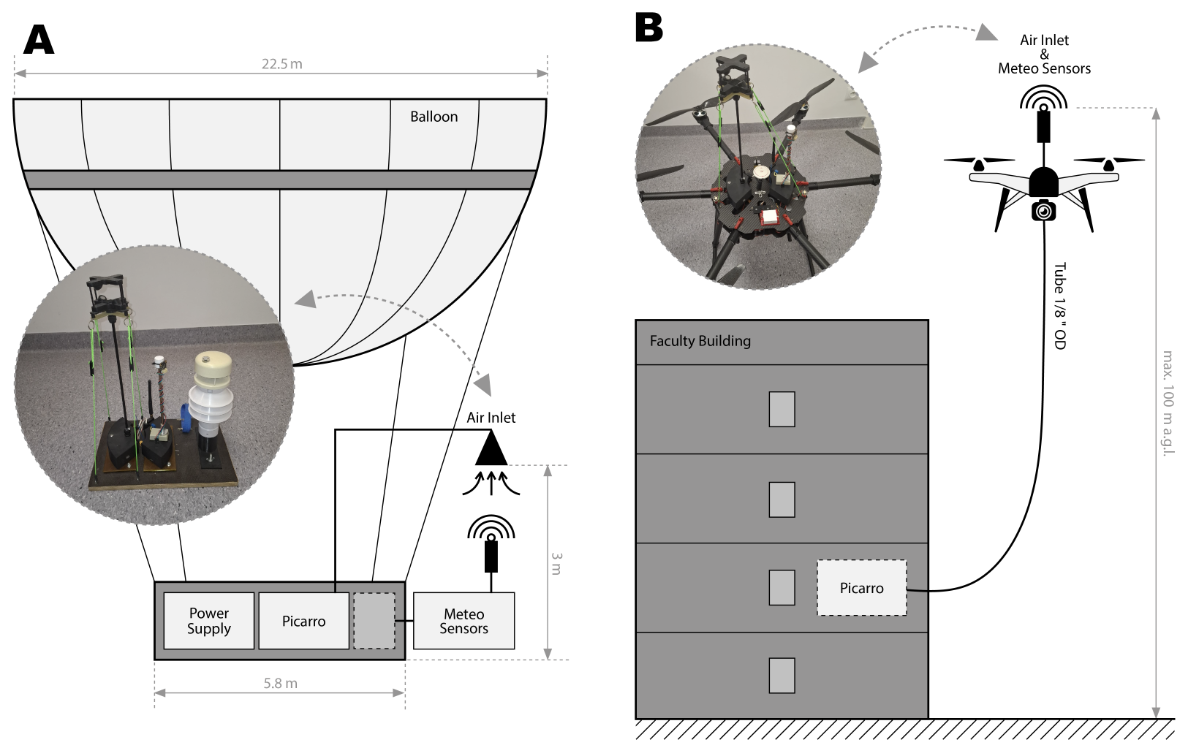
On the balloon, a set of meteorological sensors was fixed to the outer side of the passenger gondola. The Picarro G2311-f analyser and battery power supply system was placed inside the gondola, and the air inlet was installed 3 m above the gondola's deck, protruding towards the exterior by 30 cm, to avoid contamination with CO₂ exhaled by the passengers (Fig. 2A). On the UAV system, a suite of meteorological sensors consisting of air temperature, relative humidity, atmospheric pressure, and wind speed was installed on top of the UAV platform. In order to minimise the influence of turbulence generated by the propellers and provide proper ventilation of meteorological sensors and air inlet (GHG measurements), these were located in the middle part of a UAV and elevated ca. 25 cm above the propeller height (similar to McKinney et al., 2019; Hedworth et al., 2022). The air inlet at the top of the UAV was connected through a 200 m long $\mathrm{1}/\mathrm{8}$ in. OD tube to the same Picarro analyser installed in the Gas Laboratory inside the Faculty building. It should be noted that wind direction measurements were not considered in the current study due to the horizontal oscillations of the balloon during the flight. During UAV flights, the data were also rendered unusable due to the strong interference of the electronic compass with the magnetic field generated around the power cables of the UAV motors (Fig. 2B).

Figure 2 Measurement setup for platforms used in the study. (A) Balloon. (B) UAV system.

To provide detailed information on the location of the measurement, the system was equipped with a GPS receiver (NEO-7 GNSS module, u-blox AG, Thalwil, Switzerland). A detailed analysis has shown that the altitude calculated from the barometric formula (Eq. 1) is more precise than GPS measurements (Fig. S2), therefore the position was estimated using a combination of GPS and barometer signals for horizontal and vertical location, respectively.

$$\begin{array}{}\text{(1)}& h=\left[{\left({\displaystyle \frac{P}{P_{\mathrm{0}}}}\right)}^{\mathrm{1}/\mathrm{5.257}}-\mathrm{1}\right]\times {\displaystyle \frac{T}{\mathrm{0.0065}}}\end{array}$$

where: h – altitude in m a.g.l.; P₀ – atmospheric pressure at the surface level in hPa; P – atmospheric pressure at the current position in hPa; and T – air temperature at the current position in K.

In this study, only measurements collected during the ascent were considered. During the flight, the balloon often rotated and oscillated horizontally during the descent, which had a significant impact on the measurement of meteorological variables (especially wind measurements) and GHGs mole fractions under specific conditions. In the case of the ascending flight, these movements were much gentler and less frequent. Furthermore, due to the air inlet location above the balloon gondola, it was possible that the measured air might become contaminated with the passengers' exhaled air during the descent. For UAV-based measurements, a recent study by Hedworth et al. (2022) indicated that vertical measurements of gaseous pollutants during ascent are characterised by the lowest relative error (on the order of a few %), while during the descent, the relative error of measured mole fractions of gaseous pollutants may be as much as an order of magnitude higher, depending on atmospheric stability conditions.

2.2.3 Measurements of CO₂ and CH₄ mole fractions

Measurements of carbon dioxide and methane mole fractions were performed using a CRDS Picarro G2311-f analyser (Picarro, Inc., USA). For vertical profiling, the instrument operated in the flux mode (low-flow mode), enabling measurements with a precision of 0.2 ppm for CO₂ and 3 ppb for CH₄ at a frequency of 10 Hz. Before and shortly after each measurement campaign (Table 1), a calibration procedure was performed, similar to the standard procedures employed within the ICOS (Integrated Carbon Observation System) atmospheric network (ICOS RI, 2020). The calibration procedures were as follows: for 1 h, the GHG mole fractions in the two standard dry mixtures (calibration standards) of known composition were measured by the CRDS instrument. Two mixtures were selected from the cylinders available in the lab, ranging from 380 to 524 ppm for CO₂, and from 1883 to 2289 ppb for CH₄. Calibration standards consisted of two primary standards provided by the ICOS Central Analytical Laboratories (D048624, D048638) and four working standards produced in-house at AGH. All results presented here are reported in WMO GAW (Global Atmospheric Watch) scales, WMO X2019 for CO₂ and WMO X2004A for CH₄ after applying the linear calibration corrections based on calibration curves ($y=\mathrm{1.001}x+\mathrm{2.7192}$ for CO₂ and $y=\mathrm{0.996}x+\mathrm{12.109}$ for CH₄), obtained from collective calibration data obtained over all measurement campaigns. To avoid measurement contamination by human respired CO₂ during the balloon campaigns, a 10 m long $\mathrm{1}/\mathrm{8}$ in. OD inlet tube was used allowing to place the air inlet ca. 3 m above the balloon gondola. In the case of UAV campaigns 200 m long, a $\mathrm{1}/\mathrm{8}$ in. OD inlet tube was used to connect the air inlet fixed to the UAV with the stationary analyser, located in the laboratory. The Picarro pump was sufficient for flushing the tube. The inlet tubing introduced a signal delay which was determined before each campaign through a simple test performed by injecting CO₂-rich air respired by the operator and measuring the response time of the analyser (Fig. S3 in the Supplement). In the case of both species, the correlation coefficient R² for calibration lines was equal to 1 within four significant digits. The maximum long-term drift of measured standards mole fractions was 0.2 ppm for CO₂ and 1 ppb for CH₄, respectively. We applied internal instrument water correction, which is sufficient in the typically observed ranges of water vapour mole fractions (from tenths to ca. 2.5 %) (Reum et al., 2019).

2.2.4 Sensors for meteorological variables

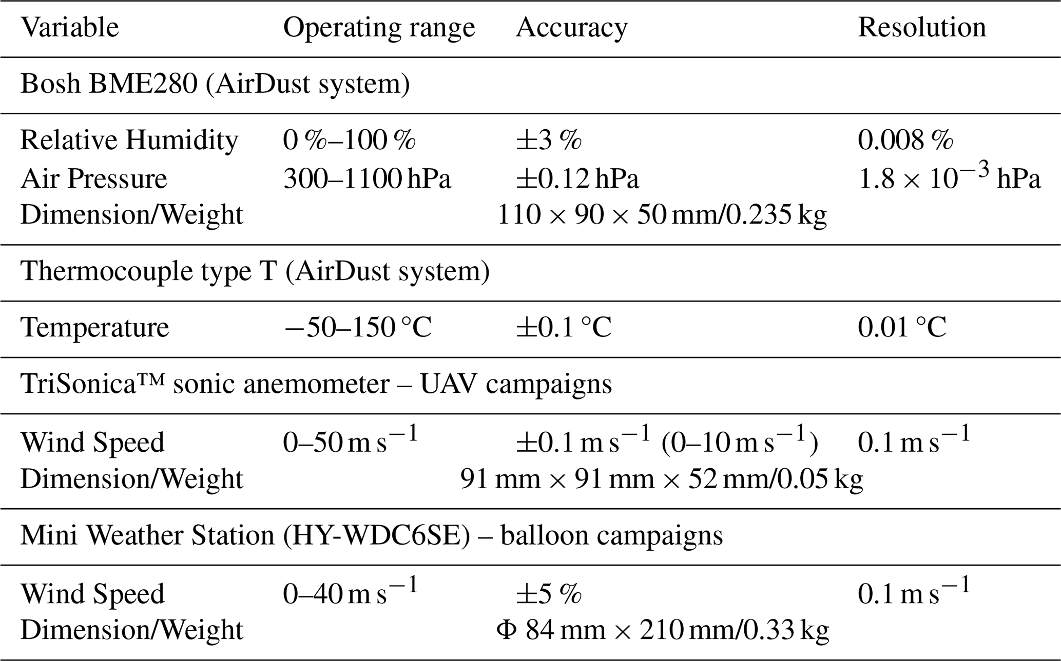
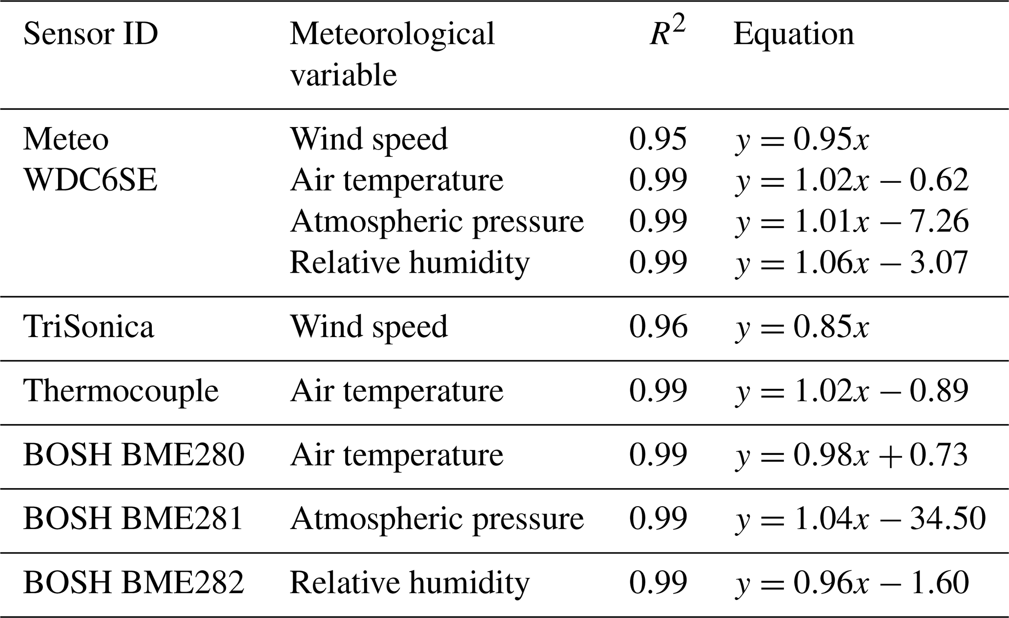
The profiles of meteorological variables presented in the article were measured using three measurement systems forming the basic set: the AirDust system (designed and constructed in-house at the Environmental Physics Group, AGH University of Krakow), the sonic anemometer TriSonica™ Mini Wind and Weather Sensor (Anemoment LLC, Longmont, CA, USA) and the Mini Weather Station (HY-WDC6SE, HONGYUV, China). The auxiliary stationary measurements are described in the next chapter. The AirDust system was dedicated for measurements with the use of both UAV (Sekuła et al., 2021c) and balloon platforms. The acoustic wind sensor TriSonica™ was used with the UAV, while the HY-WDC6SE Mini Weather Station was used in balloon campaigns. All three systems had duplicated sensors to provide redundancy during the campaigns. In the majority of flights, the temperature, pressure and relative humidity were measured using the AirDust system, while the wind speed was measured by the TriSonica Mini or HY-WDC6SE sensors. The other redundant sensors were used on per-need basis in case of primary system failure (see Table S2). The technical specification of the basic set is summarised in Table 2, and a full description of sensors, specifications and configurations are provided in the Supplement.

Table 2 Technical specifications of basic set of meteorological systems.

Calibration of all meteorological sensors was performed through a comparison against the stationary meteorological station operating at the AGH site (see Sect. 2.1 and 2.3). Air temperature, relative humidity, atmospheric pressure and wind at the level of 20 m a.g.l., were measured using a WXT520 weather station (Vaisala, Vantaa, Finland). Figure S4 in the Supplement presents a comparison between the tested sensors and reference instruments over three consecutive days (from 29 April to 2 May 2022) with 1 h resolution, together with linear regression equations for individually tested variables. The calibration equation and correlation coefficient R² obtained with the use of linear regression are presented in Table 3. For all instruments except anemometers, the formula $y=Ax+B$ was used in the calibration. For calibration of the anemometers, the intersection points of the regression lines were set to 0. Tests of the sensors showed the correct measurement for atmospheric calm (wind speed was equal to 0 m s⁻¹). Formulas of linear regression were applied to raw data to correct the systematic errors and make the measurements presented in this article consistent regardless of the specific sensor used at a given time.

Table 3 Meteorological sensors calibration details. All anemometers were calibrated using the y=Ax formula, for all other instruments $y=Ax+B$ was used.

2.3 Auxiliary in situ measurements

In addition to measurements conducted directly at the site of the measurement campaigns, continuous observations of meteorological variables and CO₂ and CH₄ mole fractions were carried out on the university campus in the location of the UAV flights providing data representing the urban boundary layer in the vicinity of the campaigns. Meteorological measurements were conducted using the Vaisala WXT520 weather station located on the roof of the Faculty of Physics and Applied Computer Science building (50.067° N 19.913° E, 20 m a.g.l.). The station has been operating at this location since 2012 and provides long-term 1 min temporal resolution information about the ambient temperature, relative humidity, atmospheric pressure, wind speed, wind direction and precipitation (see Figs. S6, S8, S10, S12, S14, S16, S18, S20, S22, S24 and S26 in the Supplement). In addition to meteorological measurements, observations of CO₂ and CH₄ mole fractions in the periods between profiling campaigns were also carried out continuously using the same Picarro analyser for profile measurements. The air inlet was placed ca. 40 m a.g.l.).

We also used the CO₂ and CH₄ atmospheric dry air mole fractions observed from the KASLAB GHG observation station at Kasprowy Wierch (49°14^′ N, 19°59^′ E, 1989 m a.s.l.) as background for the urban measurements. This station is located in the Tatra Mountains, approximately 120 km south of Krakow, and has been providing data since 1994 (Rózanski et al., 2016), and is a GAW regional station.

2.4 Estimation of urban boundary-layer height

In the subsequent analysis, for cases where clearly defined layering was identifiable, we calculated the height of the Urban Boundary Layer (UBLH) as the altitude at which measured mole fractions of the CO₂ (or CH₄) reach the value corresponding to half the difference between well-defined lowest and highest values, corresponding to either residual layer or boundary layer. We discarded five percentile of data in both extremes to account for local-scale noise. While this method has certain limitations, it is easy to apply and, contrary to thermodynamic-based methods (e.g. using the potential temperature gradient or bulk Richardson number; Kotthaus et al., 2020), it allows the layer relevant to height of mixing, most relevant in target applications concerning transport and emissions of GHGs to be calculated. The detailed algorithm of the calculation is as follows.

First, the profiles were visually filtered to exclude enhanced values in the lowest 5 m (for CO₂ those could be caused by high enhancements directly at surface likely due to the exhaled breath of crew, tourists, passers-by etc.; for CH₄ no clear cause was identified). Second, any enhancements above the UBL related to long-range transport, were excluded from the dataset as they would distort the residual layer values (see Sect. 3.3 and 3.4). Third, for each vertical profile, values below the 5th and above the 95th percentile were discarded. The remaining data formed a filtered profile dataset. In the fourth step, mole fractions of the 5th and 95th of the mole fraction value were marked as GHG_min and GHG_max, representing the residual layer or the boundary layer values. Here, the percentiles were used rather than minima and maxima to avoid distortions due to small variabilities of mole fractions within UBL and residual layer. UBLH was determined as the height at which the mole fraction profile crossed the mean of GHG_min and GHG_max. If the above condition was met multiple times for a single vertical profile, the UBLH was designated as the average of all such heights. Finally, to ensure the accuracy of the obtained boundary layer height, the profiles for a given campaign were inspected visually (together with the meteorological profiles) to exclude a limited number of events where the UBLH was identified as a false positive (afternoon flights, convective boundary layer).

3 Results and Discussion

3.1 Overview

Stationary measurements of GHGs at the AGH site (AGH University of Krakow, Faculty of Physics and Applied Computer Science, 50.067° N 19.913° E) during the period from March 2021 till April 2022 illustrate a seasonal (Fig. 3A and B) and day-to-day (Fig. 3C and D) variability of CO₂ and CH₄ respectively at the constant altitude of 40 m a.g.l. in the location close to the city centre (black symbols) compared to the regional background observed at the KASLAB high mountain station located ca. 100 km south of Krakow in the Tatra Mountains (blue symbols). The lowest monthly mole fraction of CO₂ and CH₄ was measured in May and the highest in October and are well correlated with the difference between levels observed in the UBL compared to the regional background. The annual amplitude calculated based on monthly mean values was equal to 25 ppm and 120 ppb for CO₂ and CH₄ respectively. The locations of minimum and maximum values are determined by two factors: (i) the seasonal variability of source/sink activity; and (ii) the intensity of mixing processes occurring in the UBL. A larger day-to-day change observed on the daily means recorded during the cold season is the result of the higher intensity of anthropogenic emission sources in this season and the significant influence of the synoptic situation on the daily mean values.

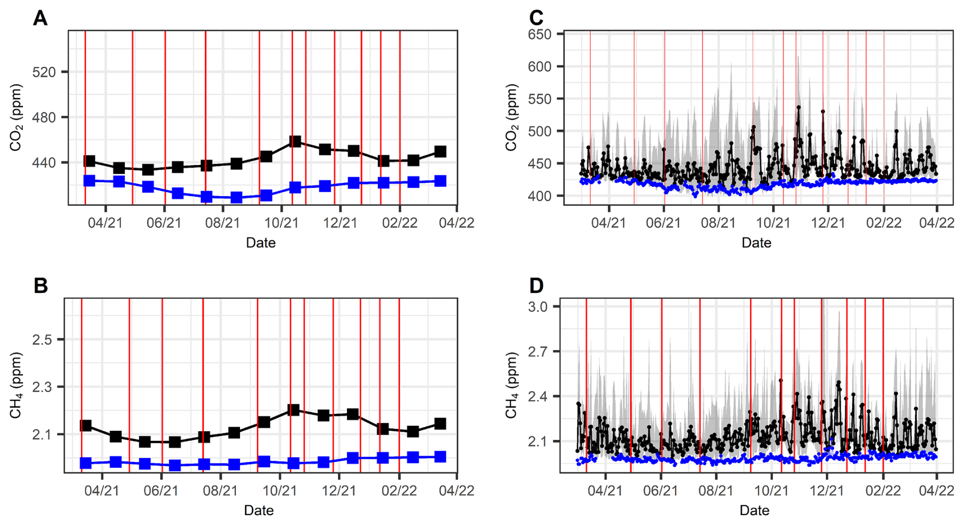
Figure 3 Monthly (A–B) and daily (C–D) means of CO₂ and CH₄ mole fractions from AGH site (dark line) at 40 m a.g.l. measured using a Picarro G-2311-f analyser and from KASLAB high-mountain station (blue line) for the period from March 2021 to April 2022. The grey shading in panels (C)–(D) indicates the diurnal variability at the AGH site, defined as the daily minimum and maximum mole fractions. The dates of vertical profile measurement campaigns are marked by vertical red lines.

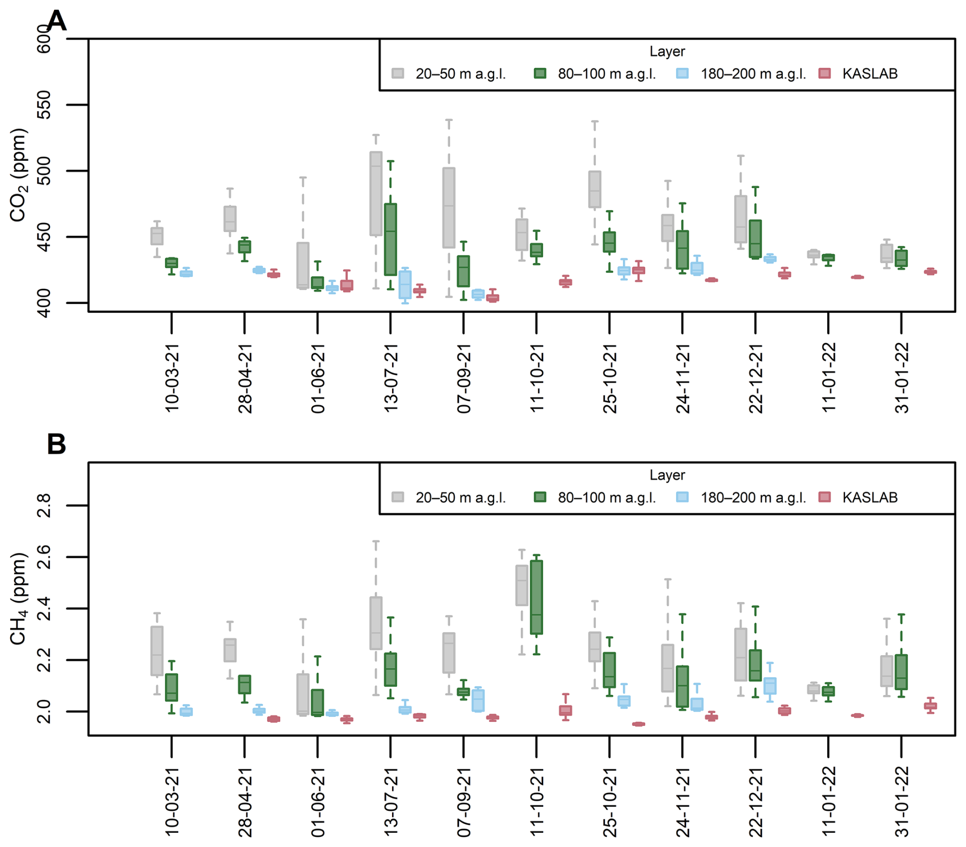
Figure 4 Box-plots of (A) CO₂ and (B) CH₄ mole fractions measured during flight campaigns at three altitude ranges (20–50, 80–100, and 180–200 m a.g.l.). The distributions are compared with background concentrations recorded at the KASLAB high-mountain station during the corresponding campaign periods.

Figure 4 presents a box and whisker plot showing the data distribution of CO₂ and CH₄ mole fractions during each campaign representing the variability observed at three different altitude ranges (20–50, 80–100 and 180–200 m a.g.l. within the city and regional background. It can be seen that the values observed in the highest layer of the urban atmosphere are close to the regional background value, but their variability is often slightly greater, which is the result of the proximity of emission sources compared to the mountain station. In turn, the highest values and the greatest variability are observed in the lowest layer. In the case of CO₂, a greater scatter of data observed in the lowest layer exists in summer compared to the winter time, while in the case of CH₄ the scatter seasonal variability is less pronounced. This suggests that methane emissions in the city originate from of a relatively constant source (leakages in the city gas network) and partly from temperature-dependent processes (like municipal waste and sewage system). The intensity of CO₂ sources in turn varies throughout the year with changes in biosphere activity (respiration and assimilation processes).

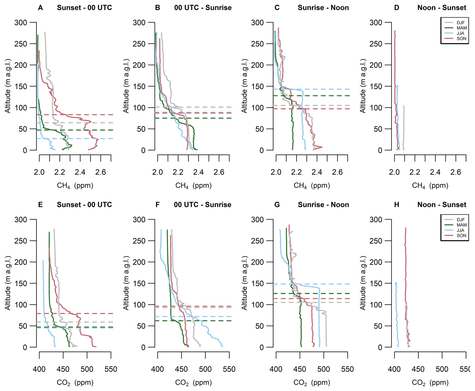
Figure 5 Selected representative CO₂ and CH₄ vertical profiles divided by season (different colours) and time of day (different columns). The selection was made to increase the readability of the graph. The whole dataset is included in the supplement for individual campaigns. Dashed lines on panels (A)–(C) indicate the boundary layer height determined separately for each individual CO₂ and CH₄ vertical profile.

Systematic measurements of CO₂ and CH₄ vertical profiles (Fig. 5) allowed us to study their variability on different timescales in the urban environment of Krakow. Distinct seasonal and diurnal variability is observed when data is filtered accordingly: by seasons (colours) and time of the day (panel columns). CO₂ mole fraction varied with altitude depending on time of day. During the day, turbulent mixing of air within the boundary layer averaged the mole fraction within the profile, and CO₂ emissions from anthropogenic and biogenic sources with their own diurnal pattern in the area were compensated by the photosynthesis sink. During the night, the diminishing of photosynthesis caused an increase in the net CO₂ flux from the surface, and as a result, together with stable boundary layer (SBL) formation, accumulation of CO₂ near the surface was observed. At the same time, CO₂ mole fraction within the higher part of the profile remained constant regardless of the time of day. The most distinct diurnal variation of the CO₂ profile occurred during the warm season, when the biosphere was most active; the highest observed difference between the surface and the free atmosphere of around 150 ppm was observed in autumn. In winter, CO₂ vertical profile varied less, with a minimum observed vertical gradient of 50 ppm. In this season, CO₂ net flux from the biosphere, which is a main driver of diurnal variability of surface emissions, is drastically diminished (Zimnoch et al., 2004), so the near-surface CO₂ mole fraction remains influenced mainly by the boundary layer diurnal dynamics. CH₄ diurnal variation has very weak seasonal dependence, with the highest observed mole fraction difference between the surface and free atmosphere of around 0.6 ppm (dark red line on Fig. 5A) and background level lowest in summer and highest in winter time (gray-winter and blue-summer lines on Fig. 5A–D). This weak variability may reflect the natural seasonal variability of CH₄ primarily controlled by its main sink – the hydroxyl radical (OH). Similarly to CO₂, BL diurnal dynamics influenced the vertical profiles of methane. It is worth emphasising that most of the profiles observed between sunset and sunrise show increased concentrations up to a height of 100 m a.g.l. which corresponds to the depth of the valley in which Krakow is located. This fact clearly illustrates the influence of local topography on the depth of the SBL in the city and the dynamics of vertical mixing of the boundary layer under stable atmospheric conditions.

A detailed BL dynamics description is included in the following sections. A full overview of the data collected in the scope of this study, grouped by campaign and augmented with meteorological data from the AGH site, is available in the Supplement (Figs. S5–S26).

3.2 Atmospheric boundary layer dynamics

3.2.1 Transition from convective boundary layer (CBL) to stable boundary layer (SBL)

Measurements collected during the vertical profiling of the UBL confirmed the key influence of UBL dynamics on the vertical profiles of CO₂ and CH₄ mole fractions. The evolution of the convective boundary layer and the development of a stable boundary layer is presented in Fig. 6 based on results from the third measurement campaign (No. 3), carried out from 1 June 2021 08:00 UTC until 2 June 2021 05:00 UTC, with a total of 44 vertical profiles sampled. Because the daytime flights were performed every 10 min, to maintain the readability of Fig. 6, only the selected profiles representing characteristic situations are presented (6 vertical profiles). During the daytime, strong vertical mixing resulted in a constant mole fraction of GHGs in the vertical profile. Between 09:00 and 16:00 UTC, the GHG mole fractions in the vertical profile ranged between 408 and 415 ppm for CO₂ and between 1.98 and 2.01 ppm for CH₄, respectively. Both values were also very close to regional background observed at KASLAB station (Fig. 7). A convective character of BL was also confirmed by the temperature profile showing a monotonic slightly negative gradient stimulating vertical mixing of BL and an almost constant wind speed ranging between 2–4 m s⁻¹ in the whole profile. After 18:00 UTC, BL dynamics changed. The wind speed gradually decreased in the lower part of the profile down to ca. 1 m s⁻¹ and the temperature gradient changed to a positive value, indicating the formation of an SBL in the first 100–150 m. This situation favoured the accumulation of emitted gases near the earth's surface and an increase of CO₂ and CH₄ mole fraction was observed close to the ground level. The vertical CO₂ and CH₄ profiles during this period were characterised by an approximately linear decrease in mole fraction up to an altitude of ca. 100 m a.g.l. After sunrise (last profile) a homogenisation of the lower atmospheric part is observed along with inversion of the temperature gradient in the first 150 m and a gradual increase in depth and a decrease in the maximum concentration at the ground, which illustrates the initiation of convective movements mixing the ground layer and carrying the gases accumulated at the surface to greater heights. The presence of an inversion aloft above 150 m, observed on the temperature profile resulted in a limitation of mixing at higher altitudes and the development of a sharp GHG gradient at the boundary between the lower convective layer and the inversion aloft. The estimated inverse height marked by a horizontal lines in Fig. 6A and B shows gradual increase from creation after sunset through development during the night until decay in the morning. The temporal evolution of CO₂ and CH₄ mole fractions averaged in three altitude ranges (30–50, 80–100, and 150–180 m a.g.l.) along with the regional background level and the marked night period, summarizing the processes discussed is presented in Fig. 7.

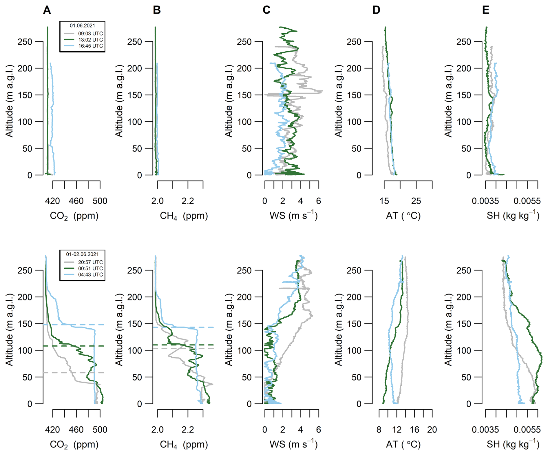
Figure 6 Selected vertical profiles of (A) CO₂ and (B) CH₄ mole fraction, (C) wind speed, (D) air temperature and (E) specific humidity for campaign No. 3 (1–2 June 2021). Dashed lines in panels (A)–(B) indicate the boundary layer height determined separately for each individual CH₄ and CO₂ vertical profile. Explanations: WS – wind speed, AT – air temperature, SH – specific humidity.

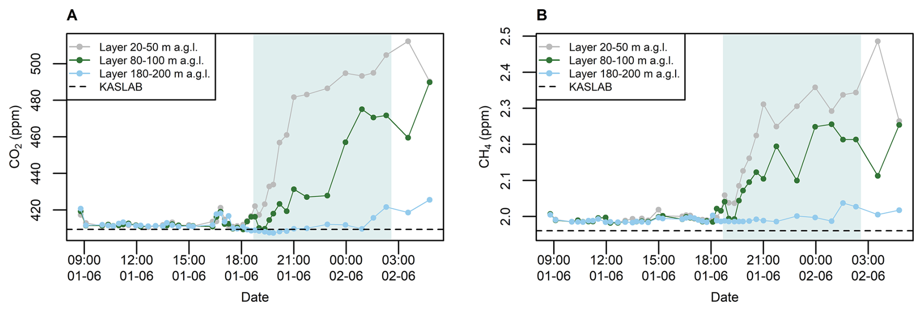
Figure 7 Time course of (A) CO₂ and (B) CH₄ mole fractions measured during campaign no. 3 (1–2 June 2021) averaged at three altitude ranges (20–50, 80–100, and 180–200 m a.g.l.). The averages are compared with regional background recorded at the KASLAB high-mountain station (dashed line) during the corresponding campaign period. Azure background presents night-time period. The regional background was calculated as the 5th percentile of 10 min averaged mole fractions from KASLAB station.

3.2.2 Transition from stable boundary layer (SBL) to convective boundary layer (CBL)

An example of the evolution from a stable boundary layer through the development of the convective layer occurring in the morning hours is better presented using data from campaign no. 7 (26 October 2021; Fig. 8). The atmospheric temperature, CO₂ and CH₄ vertical profiles show that over 5 h between 04:47 and 09:48 UTC the near-ground temperature inversion (of approximately 7 °C initially), clearly visible in the temperature profile, is gradually erased as the increasing surface temperature causes turbulence and mixing, evolving into a well-mixed lower atmosphere when surface temperatures exceed 10 °C. Initially the night-time atmosphere is clearly structured, with enhanced levels of CO₂ and CH₄ visible up to 100 m a.g.l. and distinct elevated CO₂ plumes high aloft (above 200 m a.g.l.). These high and vertically localised gradients, together with an elevated and gently varying specific humidity above 100 m a.g.l. point to a strong shear of plumes emitted upwind into a residual layer formed on the previous day, transported by varying horizontal winds, strongest at 150 m a.g.l. at 06:58 and 07:36 UTC, and reaching a maximum of 4 m s⁻¹. Over the morning, the enhancement in GHG mole fractions develops a well-mixed layer that rises together with the inversion cap, crossing 90 m a.g.l. at 08:56 UTC, and reaching approximately 180 m a.g.l. at 09:46 UTC, which is the last flight of the campaign. A complete set of profiles on that day is available in the Supplement (Fig. S17).

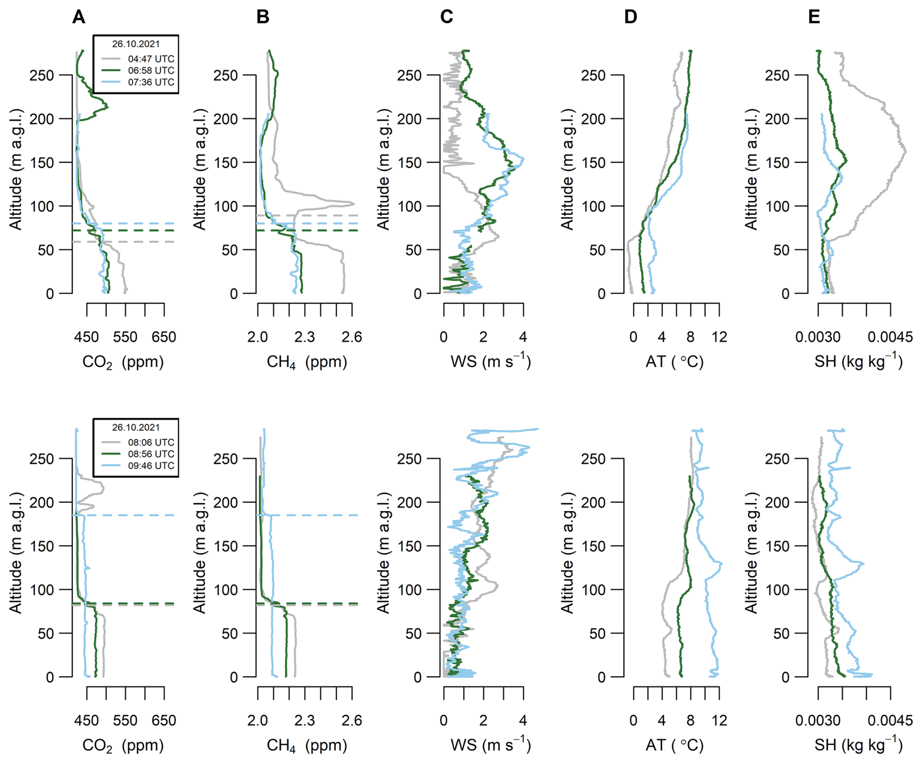
Figure 8 Selected vertical profiles of CH₄ and CO₂ mole fractions, wind speed, air temperature, and specific humidity measured during sampling campaign no. 7 (26 October 2021). Dashed lines on panels (A)–(B) indicate the boundary layer height determined separately for each individual CH₄ and CO₂ vertical profile. Explanations: WS – wind speed, AT – air temperature, SH – specific humidity.

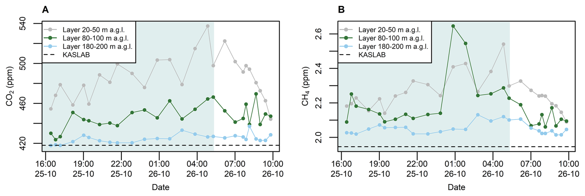
Figure 9 Time course of (A) CO₂ and (B) CH₄ mole fractions measured during campaign no. 7 (25–26 October 2021) averaged at three altitude ranges (20–50, 80–100, and 180–200 m a.g.l.). The averages are compared with regional background recorded at the KASLAB high-mountain station (dashed line) during the corresponding campaign period. Azure background presents night-time period. The regional background was calculated as the 5th percentile of 10 min averaged mole fractions from KASLAB station.

Analysis of the time course of mole fractions (Fig. 9) averaged for the lower (20–50 m a.g.l.), intermediate (80–100 m a.g.l.), and upper (180–200 m a.g.l.) layers shows a gradual increase in the lower and intermediate layers during the night, followed by a sharp decline shortly after sunrise. The levels observed in the upper layer remain close to the regional background until about 04:00 UTC, after which they begin to gradually increase, indicating the initiation of SBL degradation and the slow transport of accumulated gases to higher regions of the BL. The methane peak observed at 03:00 UTC (Fig. 9B) in the intermediate layer may indicate the detection of a plume of this gas originating from a nearby emission source whose height is within the SBL. An inconsistency observed between the CO₂ and CH₄ time course for the intermediate layer (Fig. 9A and B) clearly confirms the different origin and location of the plumes observed at the higher levels. A more detailed analysis of such observed cases can be found in the following subsections.

3.3 Anomalies in vertical distribution of GHGs – CO₂ case study

Figure 10 presents results from two measurement campaigns for which a plume of CO₂ was visible at an altitudes between 190–230 m a.g.l. (measurements from 8 September 2021) and 200–250 m a.g.l. (measurements from 26 October 2021).

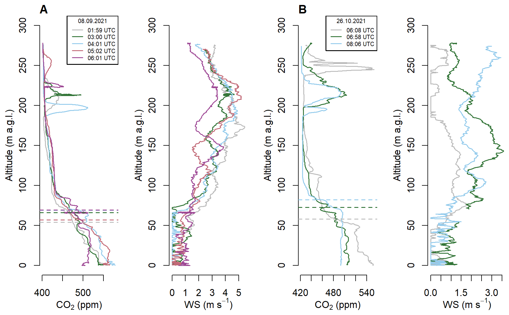
Figure 10 Vertical profiles of CO₂ and wind speed (WS) for specific hours at: (A) campaign No. 5 (flights 26–30; date: 8 September 2021) and (B) campaign No. 7 (flights 21, 22, 25; date: 26 October 2021). On both nights a plume of CO₂ was observed aloft, between 200–250 m a.g.l. Dashed lines indicate the boundary layer height determined separately for each individual CO₂ vertical profile.

The strong maxima of CO₂ mole fractions observed in the vertical profiles measured on 8 September between 01:00 and 06:20 UTC at approximately 200 m a.g.l. are clearly of different origin than gradually increasing signals closer to the surface (Fig. 10A). Such relatively thin night-time layers with strong enhancements of CO₂ are often generated by CO₂ tall stack emissions typically associated with power generation or industrial activities located upwind of the measurement point. Due to the weak vertical transport in a stable night-time atmosphere, such plumes can be transported for long distances.

Based on the prevalent wind conditions on the measurement day, as well as available knowledge on the location of the power plants in the vicinity of Krakow, we hypothesise that the observed signal originates from one of the two nearby co-generation plants, each powered by hard coal combustion. Those were Skawina PP and Krakow PP (Fig. 1). As the available measurements of wind speed and direction were sparse and variable in time and the wind patterns are often complex in the urban environment, it was not possible to identify the source responsible for observed CO₂ enhancements based on meteorological variables only.

Based on preliminary back-trajectory HySplit model calculations (Stein et al., 2015; NOAA ARL, 2026), it can be concluded that the observed plume originated from the Skawina PP (Fig. 11). Knowing the location of the emission source and terrain properties, the presented case may be a useful benchmark for testing of the vertical transport performance in the numerical atmospheric models.

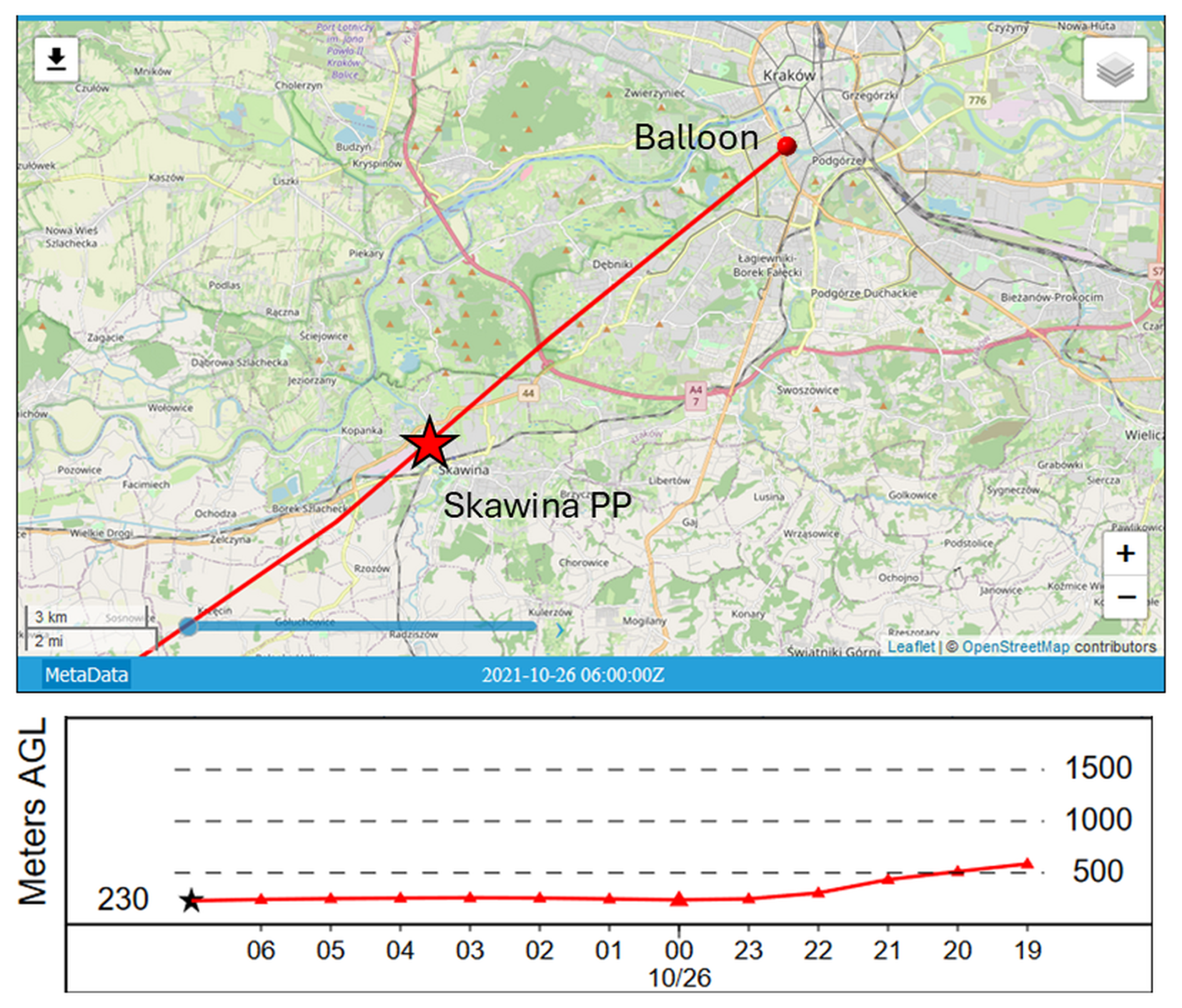
Figure 11 Hysplit back trajectory calculated using GFS0p25 meteo fields for 26 October 2021 06:00 UTC. Starting point in the balloon location at 230 m a.g.l. Position of Skawina PP marked with red star. Lower panel presents trajectory altitude.

3.4 Anomalies in greenhouse gas vertical distribution – CH₄ case study

Similar peaks were also observed in the case of CH₄ mole fraction (Fig. 12), however, the time of the detected plumes and their altitude differs from CO₂. In most cases the methane peaks appear within the SBL. This suggests that we were also able to detect the plumes emitted from a point source, but the origin and temporal dynamics of this source are different from CO₂. The lower altitude of detected peaks suggests that locations of the emissions were not associated with industrial sources emitting methane from stacks at the elevated level (as in case of the CO₂). Due to the lack of evident possible source locations, it was not possible to attribute the specific plumes to particular locations. Although the most likely source of emissions are leaks in the city gas network, or sewerage network, identification of emission sources requires further studies using model simulations with more realistic methane emission fields for the city.

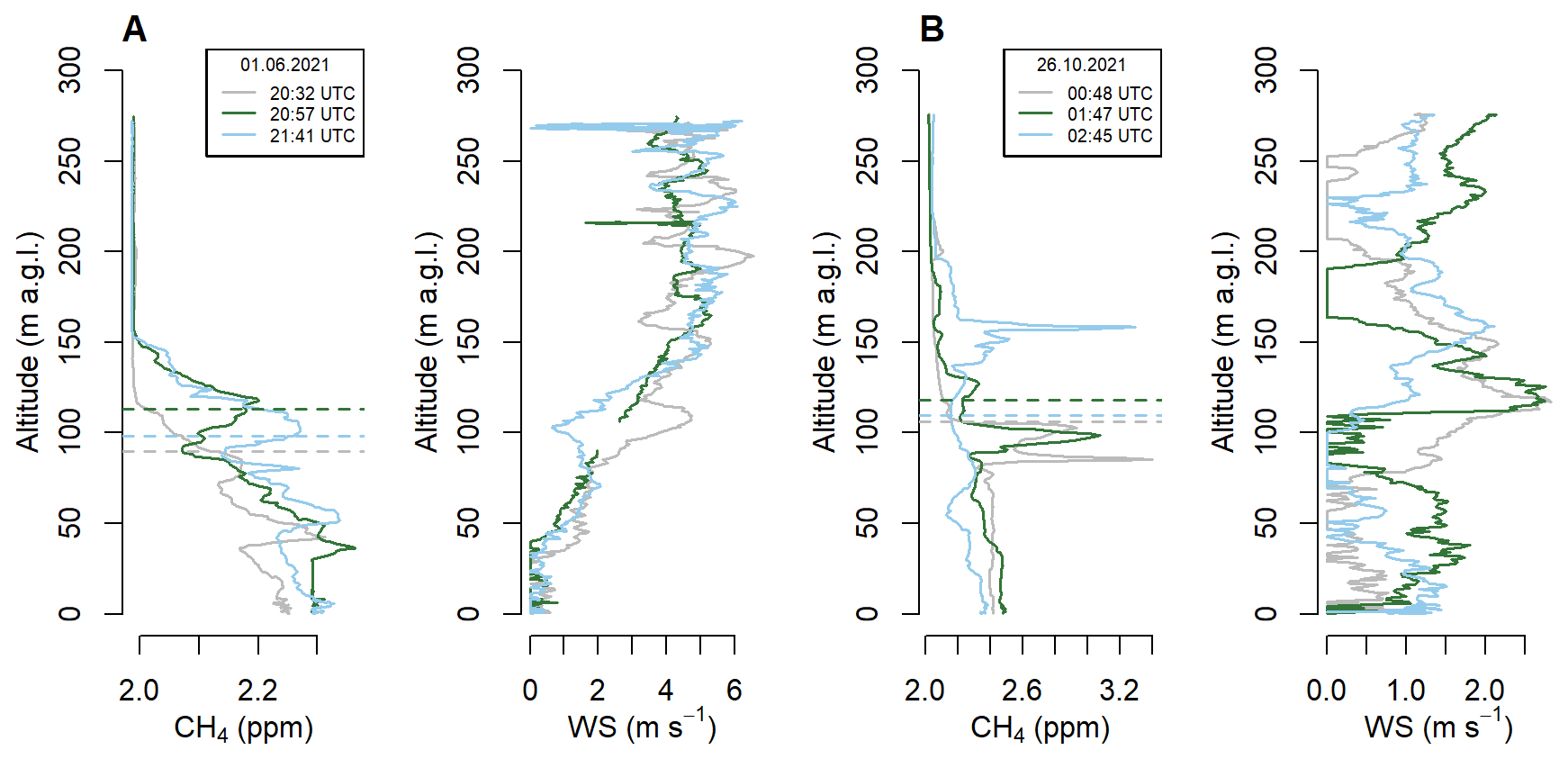
Figure 12 Vertical profiles of CH₄ and wind speed (WS) for specific hours at (A) campaign no. 3 (flights 39–41; 1 June 2021) and (B) campaign no. 7 (flights 15–17; 26 October 2021), when Gaussian plumes of CH₄ were observed. Dashed lines indicate the boundary layer height determined separately for each individual CH₄ vertical profile.

4 Conclusions

The measurement report describes 11 UBL profiling measurement campaigns conducted between March 2021 and February 2022 in the city of Krakow (Southern Poland) with approximately monthly frequency. The measurements incorporated the basic meteorological variables (temperature, relative humidity, pressure, wind speed) and CO₂ and CH₄ mole fractions recorded with 1 s temporal resolution along the profiles ranging from ground level up to 280 m a.g.l. During each campaign, several profiles were collected with at least hourly resolution covering all periods of the day, mainly focused on the formation, development and decaying of the SBL within the UBL. However, the data also illustrate the influence of terrain on the vertical distribution of trace gas contents in the boundary layer and also contain interesting point source contaminant plume data detected above and within the SBL, allowing their use to test the parametrisation of vertical transport under stable atmospheric conditions in numerical atmospheric models.

The case studies presented in this article capture clear temporal and spatial gradients, particularly within the lower PBL. The broader value of this dataset lies in its potential application for model validation. Specifically, the profiles can serve as a benchmark for evaluating regional or mesoscale transport models, offering a means to assess the performance of modelled vertical mixing, advection, and surface flux parametrisations. As such, these data contribute not only to observational insights, but also to the refinement of process-based and inverse modelling approaches within the carbon cycle research community. From the methodological point of view, we showed that carrying out profile measurements requires instruments capable of fast and precise detection of changes in measured variables (both GHG mole fractions and meteorological variables) which can change rapidly with height. In the case of measuring the wind direction, it turned out that despite corrections using an accelerometer and magnetometer, interference related to the disturbance of the magnetic field generated by powering the UAV's engines, or uncontrolled sudden rotational and lateral movements of the tethered balloon during descent caused the measurement to be unreliable.

The identification of CH₄ signals in the UBL also indicates the potential for reporting unexpected methane emissions. Identifying the specific sources needs to be done in tandem with analysis of spatial emission distribution. This can be achieved by direct analysis of the backward trajectories, as presented here. A more sophisticated approach using a full Bayesian inversion framework is in preparation.