Toward less subjective metrics for quantifying the shape and organization of clouds

As cloud sizes and shapes become better resolved by numerical climate models, objective metrics are required to evaluate whether simulations satisfactorily reflect observations. However, even the most recent cloud classification schemes rely on subjectively defined visual categories that lack any direct connection to the underlying physics. The fractal dimension of cloud fields has been used to provide a more objective footing. But, as we describe here, there are a wide range of largely unrecognized subtleties to such analyses that must be considered prior to obtaining meaningfully quantitative results. Methods are described for calculating two distinct types of fractal dimension: an individual fractal dimension D_i representing the roughness of individual cloud edges, and an ensemble fractal dimension D_e characterizing how cloud fields organize hierarchically across spatial scales. Both have the advantage that they can be linked to physical symmetry principles, but D_e is argued to be better suited for observational validation of simulated collections of clouds, particularly when it is calculated using a straightforward correlation integral method. A remaining challenge is an observed sensitivity of calculated values of D_e to subjective choices of the reflectivity threshold used to distinguish clouds from clear skies. We advocate that, in the interests of maximizing objectivity, future work should consider treating cloud ensembles as continuous reflectivity fields rather than collections of discrete objects.

1 Introduction

By resolving kilometer-scale processes, the next generation of climate models is expected to bring about a “quantum leap … in our ability to reliably predict climate” (Shukla et al., 2009). However, first it will need to be shown that the models can accurately reproduce observations of the current climate state. The challenge is that making such comparisons can be surprisingly difficult because there is no consensus on which metrics are best suited to constrain model performance (Janssens et al., 2021).

Given the climate is a physical system, any metric would ideally be something that can be linked quite directly to climate physics. Moreover, it should also be easily and accurately measurable using e.g. satellite observations, and for a sufficiently wide range of possible atmospheric states. Metrics of cloud geometries are an obvious candidate because they are readily observed from space and they are now resolvable by kilometer-scale climate models (termed Global Cloud Resolving Models or GCRMs). Clouds are also a particularly challenging test of a model, as feedbacks between cloud radiative effects and surface temperature remain the most uncertain component of model-derived estimates of the climate sensitivity (Stephens et al., 2015; Ceppi et al., 2017; Zelinka et al., 2020; Sherwood et al., 2020; Arias et al., 2021; Bock and Lauer, 2024).

Faced with the challenge of quantifying clouds' radiative impact, scientists have generally tried to “divide and conquer”, first by categorizing clouds and then identifying the physics unique to each category. The foundations of this approach can perhaps be traced to the early 19th century when Luke Howard took inspiration from the newly proposed Linnaean biological classification scheme (Howard, 1803). Using the only instrument available at the time – the human eye – Howard proposed the Latin nomenclature that still provides the dominant lens through which clouds are viewed by the atmospheric sciences community. But it is easily forgotten that Howard did not create such categories using some objective theoretical framework – rather, the categories originated from clouds' subjective appearance.

It is increasingly recognized that the properties of individual clouds are less important to the climate system than the collective impact of a cloud field (Müller and Hohenegger, 2020). Taking inspiration from Luke Howard, a new categorization system is gaining traction, this time for patterns of many clouds, using the names of sugar, gravel, fish, and flowers (Stevens et al., 2020). While differences in physical properties such as brightness temperature can be found between sugar, gravel, fish, and flowers (Bony et al., 2020), the category definitions themselves remain subjective in the first place. At first glance, any subjectivity in classification could be eliminated by developing image processing algorithms that deterministically divide clouds into pre-defined categories that align with human intuition (Bony et al., 2020). However, such objectivity is somewhat illusory given that the algorithm itself would be designed primarily to correspond with subjective cloud definitions.

As an alternative to subjective categories, here we propose that cloud fields may be better characterized by their geometry given that cloud boundaries are shaped by physics. Very generally, one of the most important physical principles is “symmetry” (Noether, 1918). In simple terms, a system displays symmetry when it does not change if the system is transformed in some way. As an example, the Navier-Stokes equations possess symmetry in time because they can be used equally well to describe today's atmospheric motions as those on some other day in the year 2100.

Less widely recognized are symmetries of spatial scale (Lovejoy and Schertzer, 2013). Namely, for some phenomenon f, scaling symmetry exists when f(x)∝f(cx) where c is a constant that “rescales” x to some other spatial scale. An example applying to clouds is the power-law distribution of cloud areas. Satellite observations show that the number of clouds n scales as their area a through $n\propto a^{-\mathit{\alpha }}$ with a nearly constant exponent over at least 6 orders of magnitude (Wood and Field, 2011; DeWitt et al., 2024). The distribution respects a scaling symmetry because, if the scale under consideration – in this example cloud area – were to be changed through multiplication by a constant c, then the number of clouds is rescaled by some other constant c^−α. On Earth, due to the finite size of the planet and the finite size of cloud droplets, symmetry cannot apply to an infinite range of scales. Nevertheless, for the range over which it applies, scaling offers an important simplification: cloud geometries observed at any one scale can shed light on their geometries at (nearly) any other scale.

The aim here is to introduce simple and objective metrics for defining the geometries of clouds and cloud fields. We focus on cloud size and shape, and explore the applicability of fractal metrics from the standpoint of satellite observations (Sect. 2). Our methods are also easily applied to climate model output. Not all of the metrics we discuss are novel, as various fractal dimensions and size distribution exponents have previously been used to classify individual cloud types such as cirrus and cumulus (Batista-Tomás et al., 2016), cloud field types such as sugar and gravel (Janssens et al., 2021), and compare simulated and observed clouds (Siebesma and Jonker, 2000; Christensen and Driver, 2021; Raghunathan et al., 2025). Fractal metrics have also been shown to intimately reflect atmospheric dynamics – specifically, an anisotropy between the horizontal and vertical dimensions of atmospheric turbulent flows (Rees et al., 2024). But, as we show in Sect. 3 there are important pitfalls to fractal dimension analyses that have been almost entirely overlooked in prior literature.

Specifically, the fractal dimension of clouds is most commonly determined from a relationship between individual cloud perimeter and area, as first introduced by Lovejoy (1982). The strict mathematical definition of a fractal dimension, however, is defined by the relationship of an object's perimeter to the measurement resolution (Mandelbrot, 1982). The justification for Lovejoy's method has its origin in a very brief derivation by Mandelbrot (1982). We show here that the two approaches are only equivalent if certain very strict geometric conditions are satisfied, and that these conditions do not apply well to natural clouds. Another difficulty, described in Sect. 4, is the fact that fractal dimensions may be defined with respect to either individual clouds or ensembles of clouds, and this decision strongly affects the resulting values. We suggest that the “ensemble” fractal dimension may prove particularly useful for characterizing cloud fields as it quantifies relationships between clouds of different sizes in a way that the more common “individual” fractal dimension does not.

We also aim to examine and improve the methodologies by which the fractal dimensions are calculated in order to give future model intercomparison or cloud classification studies better tools. A particular appeal of fractal metrics is that the values characterize statistical relationships between scales rather than statistics at any particular scale, for example enabling more straightforward comparisons between observations or models with differing resolutions. But for such benefits to be realized, the metrics must be accurately calculated in the first place such that their values do not depend on the particulars of domain size or dataset resolution. When accurately measured, fractal metrics instead reflect the underlying symmetry of spatial scale present in cloud fields and the physics governing Earth's atmosphere more broadly.

2 Datasets

To analyze the geometries of cloud fields, we use a calibrated optical reflectance product R from MODIS that is sensitive to visible wavelengths between 620 and 670 nm (Band 1). The dataset has a nadir resolution of 1 km, increasing to roughly 2 km at a sensor zenith angle of 60°. We only consider the portion of the swath that has a sensor zenith angle of 60° or less. Each image or granule considered here covers a domain that is roughly 1950 km wide by 2030 km long and was collected during January 2021 between 60° S and 60° N. “Cloud masks”, defined as binary images distinguishing cloudy from clear sky, are created by setting each pixel with R greater than a set threshold to cloudy and the rest to clear. A range of thresholds are considered between R=0.1, permitting detection of nearly all visible clouds, to R=0.35, which allows only the most highly reflective convective cores to be detected (Fig. 1). Additional thresholds were also tested (Appendix C) but they resulted in too few clouds for robust statistical analyses.

To reduce contamination from bright objects that are not clouds, images are only considered if they are at least 99.9 % over water and contain less than 10 % sun glint (Ackerman et al., 1998). To ensure that the entire domain is visible in full daylight, granules are omitted if any portion has a solar zenith angle larger than 70°. These criteria are chosen as a compromise between a sufficiently large sample size and ensuring accurate measurements. The result is a total of 72 images. As shown in the Supplement, computed parameter values can vary for individual images but converge when computed over roughly 10–15 randomly selected images. This indicates that the parameter values computed here, obtained using all 72 images, represent their climatological values.

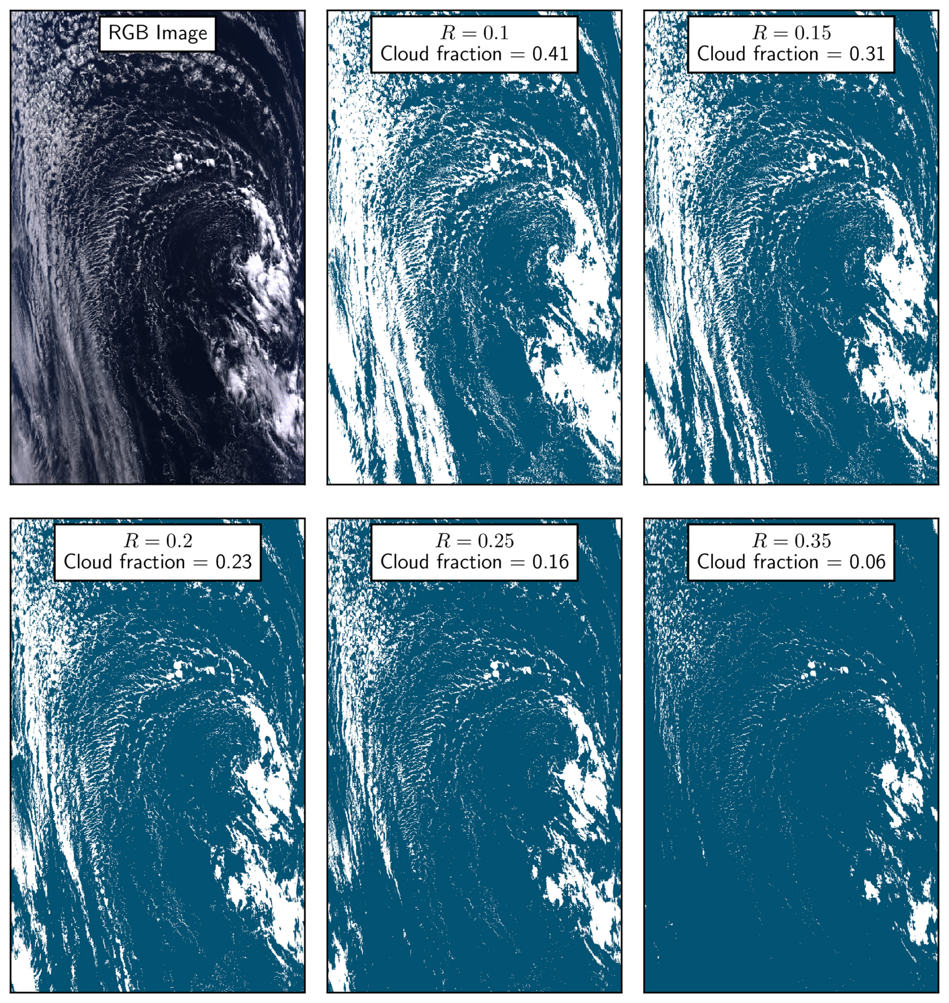
Figure 1 Example cloud masks generated using a selection of thresholds in optical reflectance R, compared to an RGB image. The image shown was taken on 1 January 2021 at 14:00 UTC, and is centered at approximately 29.1° N, 48.6° W.

Individual clouds are defined as contiguous groups of adjacent cloudy pixels. Diagonally positioned pixels are not considered to be contiguous (Kuo et al., 1993). Pixels are not uniform in size because the distance between a cloud and the viewing satellite can change, and also because each cloudy pixel is viewed at an angle. With appropriate adjustments for viewing geometry, perimeters p are calculated by summing contiguous pixel edge lengths along the boundary of each cloud, and areas a by summing the area of each cloudy pixel within the cloud. Contortions along cloud edges are unresolved for the very smallest clouds (Christensen and Driver, 2021), so clouds with a<10 km² are omitted from calculations of the fractal dimension of individual clouds (Sect. 3.2), and clouds with p<10 km are omitted from perimeter distribution calculations (Sect. 4.3). Throughout, power-law exponents are computed using ordinary least-squares linear regressions to logarithmically transformed variables, and all reported uncertainties represent twice the standard error of the fitted slope (i.e. a 95 % confidence interval).

3 Determination of the individual fractal dimension D_i

3.1 Theory

The original definition of the fractal dimension D_i as proposed by Mandelbrot (1982) is that an individual cloud with perimeter p_i can be related to a variable “ruler length” or resolution ξ through

$$\begin{array}{}\text{(1)}& {\displaystyle }{p}_{\mathrm{i}}\propto {\mathit{\xi }}^{\mathrm{1}-D_{\mathrm{i}}}.\end{array}$$

Provided D_i is not a function of ξ, the object can be termed to be “self-similar” because the measured quantity p_i is a power law function of the chosen spatial scale ξ respecting a symmetry of spatial scale. Visually, self-similarity implies that the shape of an object such as that shown in Fig. 2 repeats at many different spatial scales. Such exact repetition is not present in clouds, but there is still a sense in which small-scale cloud edge contours appear similar to their larger-scale counterparts. To precisely capture this appearance, we may modify the concept of self-similarity to only require that the statistics of the patterns – rather than the exact pattern – be similar across scales. This broader notion was termed “statistical self-similarity” by Mandelbrot (1967). More specifically, statistical self-similarity exists when

$$\begin{array}{}\text{(2)}& {\displaystyle }〈p_{\mathrm{i}}〉\propto {\mathit{\xi }}^{\mathrm{1}-D_{\mathrm{i}}}\end{array}$$

where the average is taken over some large collection of clouds with uniform size but not necessarily uniform perimeter (Fig. 3). The requirement of uniform size is intended to isolate changes in perimeter that are due solely to changes in the “roughness” of cloud edge, or the fractal dimension (Fig. 2; Imre, 1992). Size here is defined as a property that, unlike perimeter, is not a function of resolution. It could be defined in a number of ways, but for simplicity of argument's sake (as discussed in more detail below) we start by defining size as the cloud bounding box width l (Fig. 3).

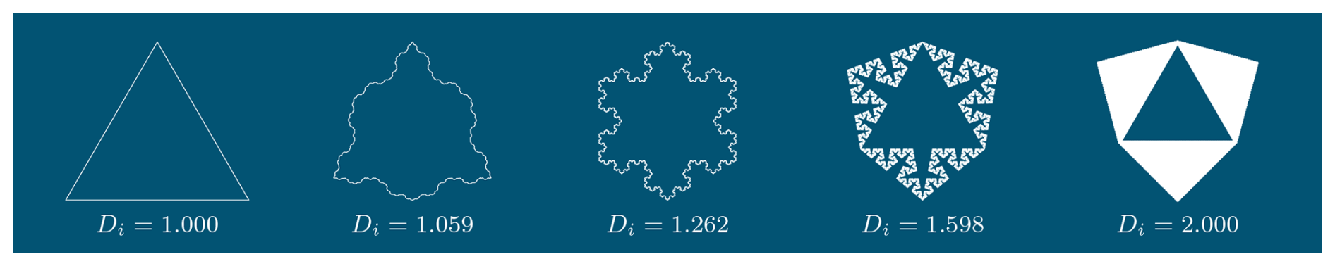
Figure 2 A generalized version of a self-similar Koch snowflake for varying fractal dimensions.

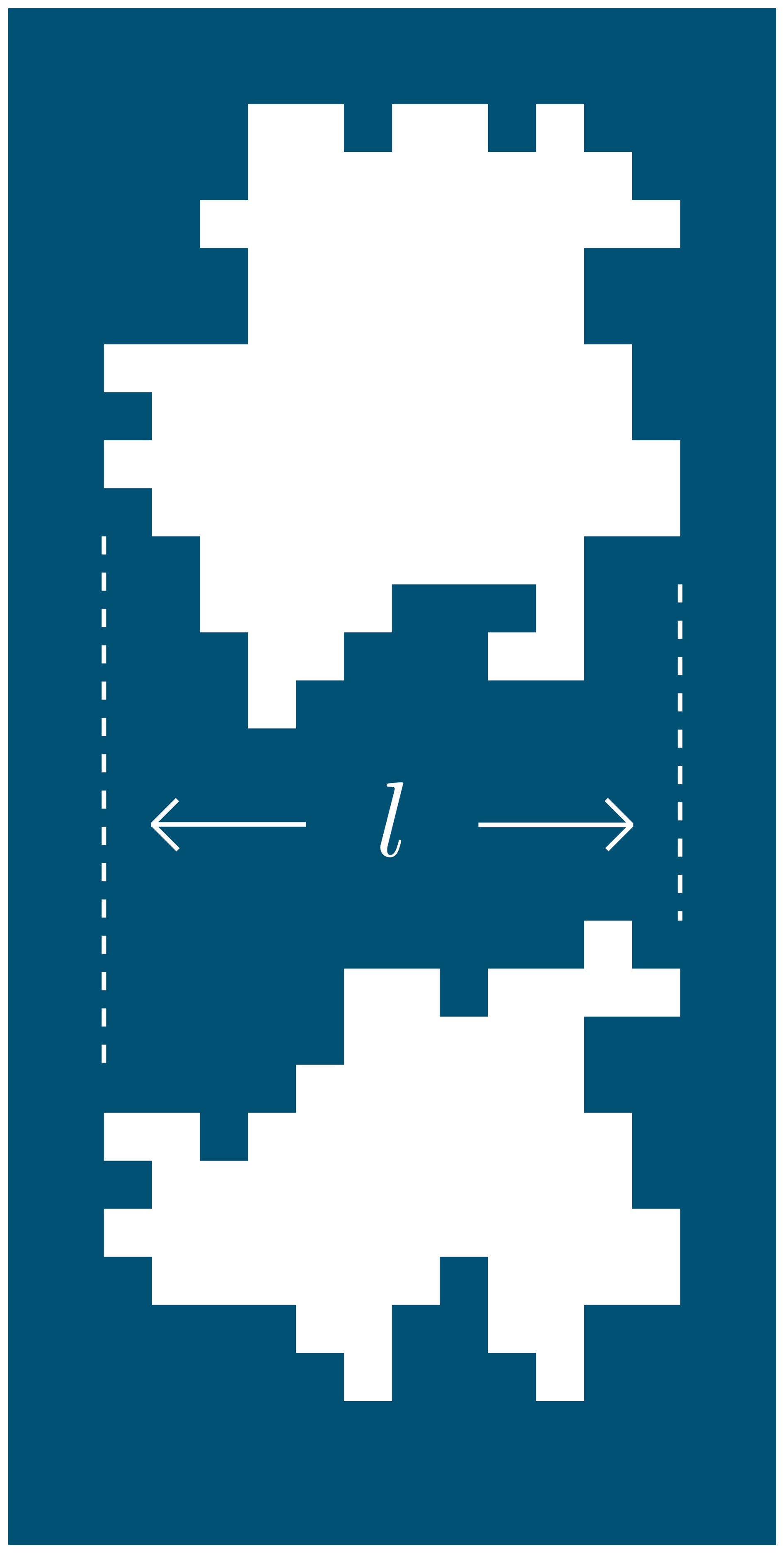
Figure 3 Two clouds may have different perimeters even if they have the same size l, defined here as bounding box width, and are measured at the same resolution ξ.

It is difficult to apply Eq. (2) directly to satellite images of cloud fields because clouds encompass a wide range of sizes and types, not to mention that satellite images are obtained at a fixed image resolution. It is for this reason that a different expression is usually used to determine the fractal dimension, one that relates satellite measures of individual cloud perimeters p_i to their areas a_i (Lovejoy, 1982; Henderson-Sellers, 1986; Bazell and Desert, 1988; Gifford, 1989; Cahalan and Joseph, 1989; Jayanthi et al., 1990; Sengupta et al., 1990; Chatterjee et al., 1994; Gotoh and Fujii, 1998; Siebesma and Jonker, 2000; Luo and Liu, 2007; Peters et al., 2009; von Savigny et al., 2011; Brinkhoff et al., 2015; Batista-Tomás et al., 2016; Christensen and Driver, 2021), namely

$$\begin{array}{}\text{(3)}& {\displaystyle }{p}_{\mathrm{i}}\propto a_{\mathrm{i}}^{D_{\mathrm{i}}/\mathrm{2}}.\end{array}$$

In this case, D_i is estimated from a simple linear fit to a scatterplot of the easily calculated quantities of log p_i and $\log \sqrt{a_{\mathrm{i}}}$.

Equation (3) for the fractal dimension is very different in form than the strict definition given by Eq. (2). As justification, Lovejoy (1982) referred to the work by Mandelbrot (1982) (p. 110), where it was proposed that the two expressions are interchangeable. It is worth reviewing Mandelbrot's subtle argument in more detail because, as we will show, its assumptions do not strictly apply to clouds.

On an intuitive level, any given cloud in a cloud field can be considered to have two independent geometric properties: size and shape. By shape, we mean the roughness or complexity of the cloud boundary, which is perhaps the most visually notable aspect that differentiates clouds, such as those shown in Fig. 1. To quantify cloud shape, suppose a subset of clouds within the field, chosen such that each cloud has the same size l_i but with varying perimeter p_i. This collection, represented by panel (a) in Fig. 4, could be used to calculate the fractal dimension. One would “resample” each cloud by increasing ξ, creating a collection of coarsened images as in panel (b). Such a resampling process would change each cloud's shape as finer contours are no longer resolved in the coarsened images. Using a range of values for ξ and the resulting range of perimeters 〈p_i〉(ξ) at each resolution, D_i could then be obtained from a fit to Eq. (2).

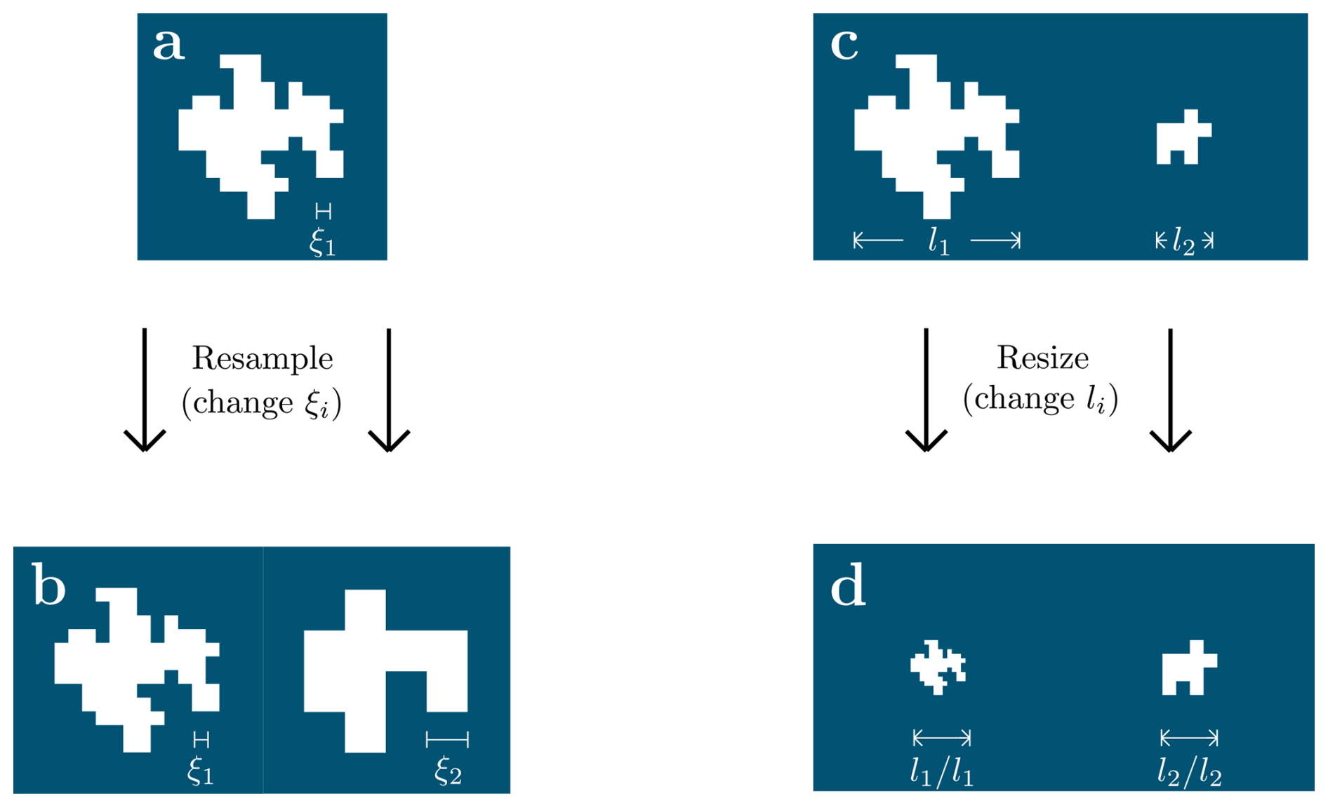
Figure 4 Self-similarity for a cloud field defined as an equivalence between the fractal dimension D_i calculated from “resampled” (a, b) and “resized” (c, d) images of clouds. The right cloud in (b) was obtained from (a) by coarsening the resolution ξ by a factor of 3, obtaining a collection of clouds (b) at varying resolutions as required by Eq. (2). In contrast, the collection (d) was obtained by resizing two originally different clouds (c) such that their size l_i is uniform. Self-similarity implies that fractal dimensions calculated from both (b) and (d) are the same.

Alternatively, the size could be varied as the shape stays the same. D_i could be calculated from Eq. (1) by taking a collection of clouds having a range of sizes l_i, as in panel (c), and then resizing each cloud by normalizing the image width and height dimensions by the cloud size, effectively zooming the image. Although all clouds were originally imaged with the same resolution, the “larger” clouds, once resized, would appear to have a finer resolution than the smaller clouds. In fact, all length dimensions would change during resizing by the same factor $\mathrm{1}/l_{\mathrm{i}}$, including image width, cloud size, resolution, and perimeter. The resized clouds therefore have size $l_{\mathrm{i}}/l_{\mathrm{i}}=\mathrm{1}$, resolution ${\mathit{\xi }}_{\mathrm{i}}/l_{\mathrm{i}}$, and perimeter $p_{\mathrm{i}}/l_{\mathrm{i}}$. The fractal dimension D_i could then be calculated by substituting the normalized perimeters and resolutions into Eq. (1), leading to the expression $p_{\mathrm{i}}/l_{\mathrm{i}}\propto {\left({\mathit{\xi }}_{\mathrm{i}}/l_{\mathrm{i}}\right)}^{\mathrm{1}-D_{\mathrm{i}}}$ or

$$\begin{array}{}\text{(4)}& {\displaystyle }{p}_{\mathrm{i}}\propto {\mathit{\xi }}_{\mathrm{i}}^{\mathrm{1}-D_{\mathrm{i}}}{l}_{\mathrm{i}}^{D_{\mathrm{i}}}.\end{array}$$

The size metric l_i must have dimensions of length given that it is used to normalize the length quantities p_i and ξ_i.

Thus, there are two methods that can be used to calculate D_i for a collection of clouds: resampling by varying shape and resizing by varying size. If the two methods yield the same value, then the clouds exhibit statistical self-similarity as defined above. Note that, provided the field is self-similar, calculating D_i by resizing has the advantage of enabling a more statistically robust fit. This is because any cloud in the field can be resized by normalizing by its size l_i, whatever its original size, and so the number of clouds that can be considered is much larger than if only resampled clouds of some fixed size are considered.

For the length dimension l_i, Mandelbrot (1982) proposed that the square root of the cloud area could be used, making the assumption that the cloud area is proportional to the area of the smallest bounding box a_BB. If so, Eq. (4) becomes Eq. (3). However, Mandelbrot's assumption that a_i∝a_BB requires that cloud area is not a function of resolution because a_BB is not a function of resolution. If cloud area does in fact change with resolution, it would certainly be possible to calculate a statistical fit of p_i to a_i that yields a value of D using Eq. (3). But, this value of D cannot be interpreted to be a fractal dimension defining the geometric properties of the cloud field (Imre, 1992), at least not one consistent with the original definition of the fractal dimension given by Eq. (1). It is not even clear what the correct interpretation should be.

3.2 Measurements

Are Mandelbrot's assumptions valid for clouds such that Eq. (3) is justified as a substitute for Eq. (1)? One potential issue is that clouds viewed from space have interior holes where the underlying surface can be viewed beneath. Resampling the cloud at a coarser resolution would cause the cloud holes to disappear so that $\sqrt{a}$ becomes an increasing function of ξ. Cloud areas would not be resolution independent, and so the perimeter-area relationship given by Eq. (3) would not strictly hold. If a fit were calculated using Eq. (3) regardless, the calculated fractal dimension would be larger for large clouds that have more holes. Such an increase of fractal dimension with cloud size has in fact been observed in several prior studies (Cahalan and Joseph, 1989; Gifford, 1989; Sengupta et al., 1990; Benner and Curry, 1998).

To test whether the observed dependence of fractal dimension on cloud size is a real property of the clouds, or it is instead a consequence of a false assumption that cloud area is resolution independent, any cloud holes could be filled to define a “filled area” a_f (von Savigny et al., 2011; Brinkhoff et al., 2015; Batista-Tomás et al., 2016). If instead Mandelbrot's assumption that cloud area is independent of ξ holds for clouds, then filling the holes should not be expected to affect the calculated fractal dimension. To illustrate, consider the case where filling cloud holes increased every cloud's area by a constant factor c such that a_f=ca. This would not affect D_i because the coefficient $D_{\mathrm{i}}/\mathrm{2}$ relating log p to log a on a scatter plot of cloud sizes would remain unchanged.

Figure 5 shows such a comparison between cloud perimeter and the square root of area, for filled and unfilled clouds observed using MODIS as described in Sect. 2. In the imagery, filled areas a_f and filled perimeters p_f are calculated by first identifying all contiguous clear regions that are not connected to the largest contiguous clear region in the image (the clear-sky “background”), and then assigning those interior regions, or holes, as being cloudy. Then, a_f and p_f are calculated from the hole-filled cloud mask in an equivalent manner as a and p as described in Sect. 2. To determine any size dependence of fractal dimension calculated from Eq. (3), regressions between log p and $\log \sqrt{a}$ are divided into four different decades in cloud area: 10 to 10², 10² to 10³, 10³ to 10⁴, and 10⁴ to 10⁵ km².

Figure 5 shows that the “unfilled” fractal dimension has a higher value than the “filled” dimension at all scales (a similar observation has been made of noctilucent clouds by Brinkhoff et al., 2015). More importantly, the unfilled dimension increases from 1.41±0.01 for the smallest cloud size class to 1.87±0.18 for the largest cloud size class. By contrast, the filled fractal dimension displays substantially less scale dependence, ranging only from 1.36±0.01 to 1.55±0.13.

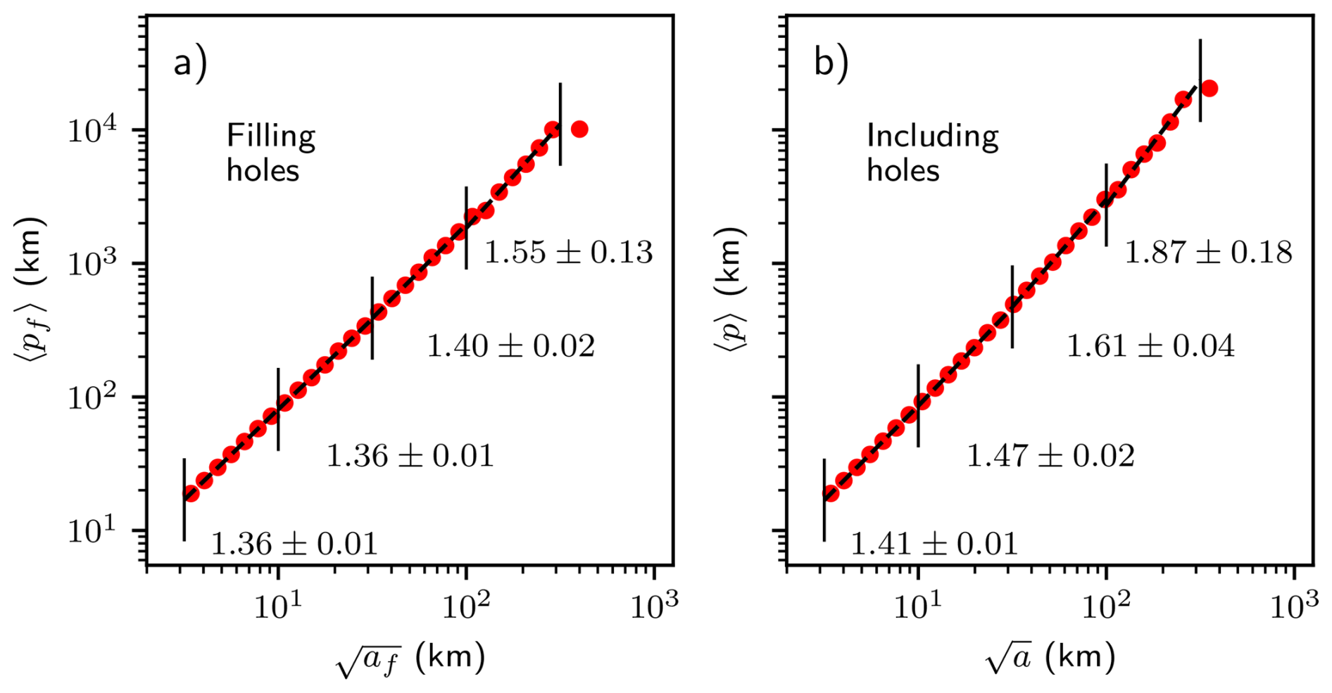
Figure 5 Dependence of the individual cloud fractal dimension on scale for clouds with holes filled (a) and without filling holes (b) for a threshold R=0.1. The perimeters p_f and areas a_f are obtained from clouds after any holes are filled in, while p and a are calculated as described in Sect. 2. Each point represents the mean perimeter in a logarithmically-spaced area bin. The listed fractal dimensions D_i are calculated using regressions (dashed lines) to four different size ranges delineated by the vertical black lines.

For filled clouds, calculated values of D_i change minimally with the reflectance threshold R as shown in Fig. 6. For six different thresholds ranging from R=0.1 to R=0.35, D_i only ranges from 1.38±0.02 to 1.40±0.01. Values of D_i are consistent with values obtained in the minority of prior studies of cloud fractal properties that explicitly mentioned that cloud holes were filled (von Savigny et al., 2011; Batista-Tomás et al., 2016).

To summarize, a fractal dimension D_i defining a collection of clouds may be calculated from a perimeter-area relationship through Eq. (3), in which case it offers a succinct metric for understanding cloud dynamics or for evaluating or comparing measurements and models. However, for the perimeter-area exponent to represent a true “dimension” mathematically, there is an a priori requirement that cloud areas not be a function of sampling resolution. This mathematical requirement can be satisfied, but only if cloud holes are filled, a procedure that might be argued to neglect an important physical property of the cloud field.

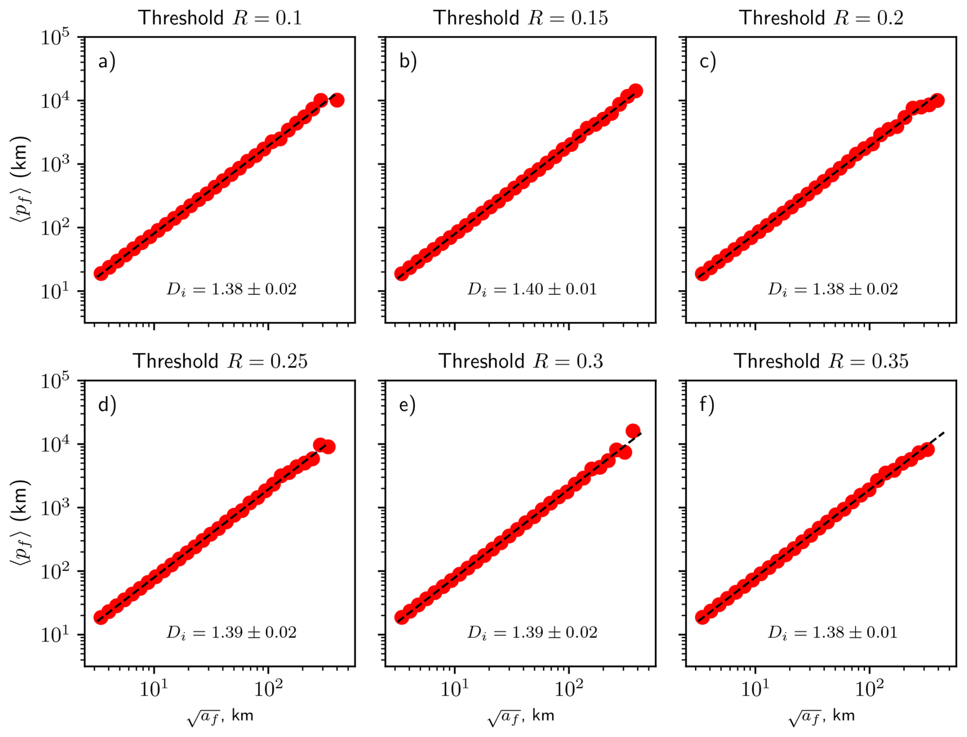
Figure 6 Calculations of the individual cloud fractal dimension D_i for a range of cloud thresholds in reflectance R. Each point represents the mean filled perimeter 〈p_f〉 in a logarithmically-spaced bin of filled area a_f. Values for D_i are obtained as a linear regression to $\log \sqrt{a_{\mathrm{f}}}$ vs. log 〈p_f〉.

4 The ensemble fractal dimension

4.1 Theory

An alternative approach for defining the fractal properties of a cloud field according to Eq. (2) is to employ what we term the “ensemble fractal dimension” D_e. The mathematical definition is analogous to Eq. (1), but with the mean cloud perimeter 〈p_i〉 being replaced by the total cloud perimeter P:

$$\begin{array}{}\text{(5)}& {\displaystyle }P=\sum _i{p}_{\mathrm{i}}\propto {\mathit{\xi }}^{\mathrm{1}-D_{\mathrm{e}}}.\end{array}$$

This definition of the ensemble fractal dimension was employed by Rees et al. (2024) to demonstrate, using satellite observations, that the turbulent properties of the atmosphere are not 2D at large scales and 3D at smaller scales as is commonly supposed (Nastrom et al., 1984). In Appendix A, we show that D_e captures two orthogonal effects: individual cloud edge complexity and the size distribution of clouds in the field.

Curiously, where most past studies only measured D_i (Lovejoy, 1982; Cahalan and Joseph, 1989; Siebesma and Jonker, 2000; Peters et al., 2009; Yamaguchi and Feingold, 2013; Christensen and Driver, 2021), some have in fact determined D_e without discussion of how the two measures differ (e.g. Lovejoy et al., 1987; Carvalho and Dias, 1998; Janssens et al., 2021). By considering the lengths of idealized island coastlines, Mandelbrot (1982) made the distinction clear: the ensemble fractal dimension D_e applies when “lumping all the islands' coastlines together”.

For a better understanding of the numerical distinction between D_i and D_e, consider again that cloud fields have the combined properties of size and shape as shown in the idealized cloud field shown in Fig. 7. Given that increasing the fractal dimension of any single cloud increases its perimeter, and therefore the total P, we can see that D_e increases if D_i increases. However, there is the added consideration of the relative numbers of small and large clouds – a subject now of considerable interest for studies of convective cloud organization. To see how, consider re-drawing some cloud field such that the number of small clouds increases while maintaining a fixed total cloud area, for example by dividing a few large clouds into a larger number of smaller ones. Necessarily, this too would increase the total perimeter, since one would need to draw additional cloud edges to divide up the cloud. Precisely how much P changes depends on the change to the cloud size distribution. From observations spanning a wide range of cloud sizes and climate states (DeWitt et al., 2024), a reasonable assumption is that the distribution follows a power-law distribution with some exponent β such that

$$\begin{array}{}\text{(6)}& {\displaystyle }n\left(p\right)\propto p^{-(\mathrm{1}+\mathit{\beta })}\end{array}$$

where the total number of clouds N is given by $N\propto {\int }_{p_{\text{min}}}^{p_{\text{max}}}n\left(p\right)\mathrm{d}p$. In this case, a field with a large number of small clouds relative to large clouds would have a larger value of P and a higher value of β, assuming the total cloud area remains unchanged. An example showing this dependence is shown along the ordinate of Fig. (7).

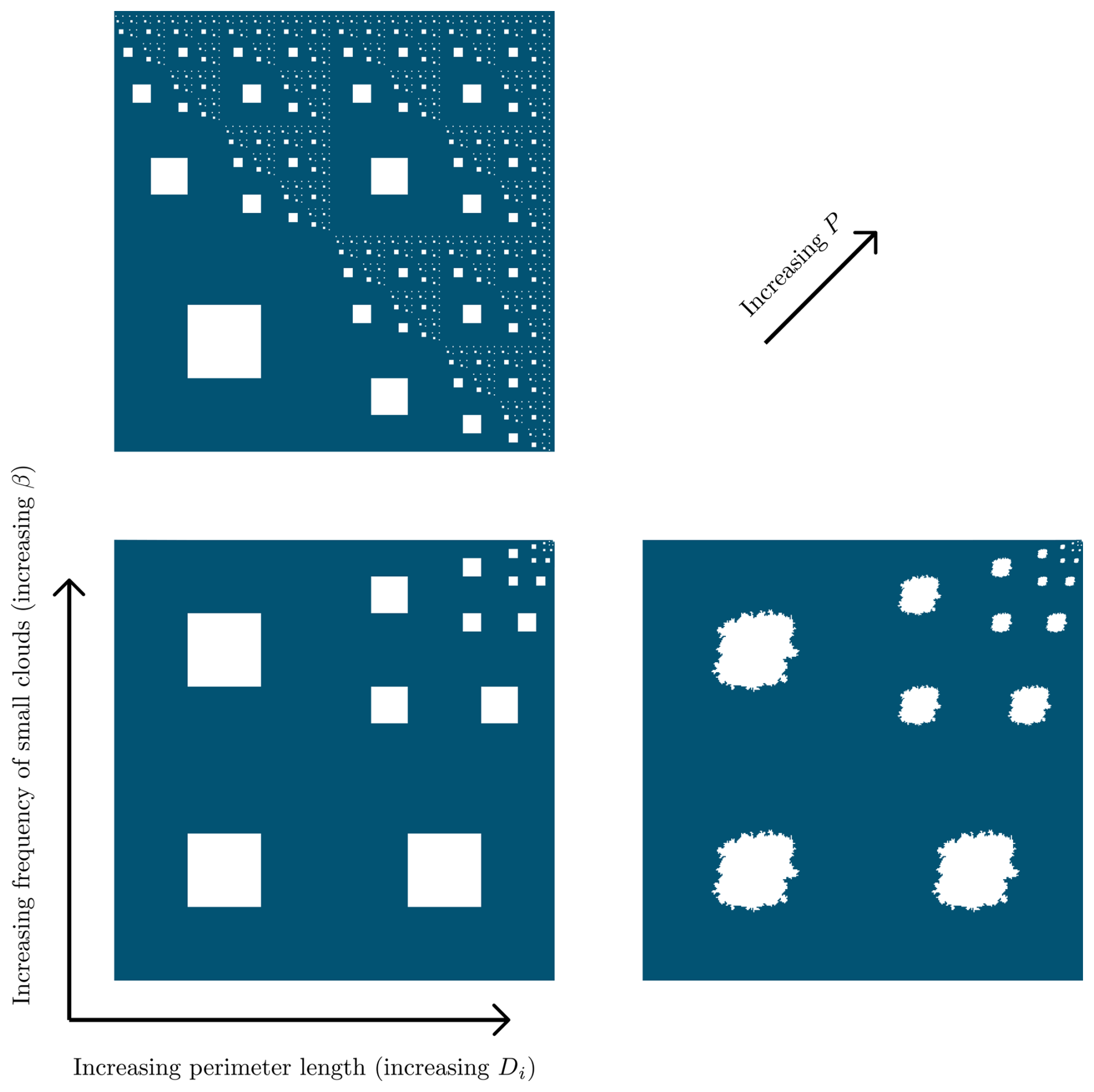
Figure 7 For a constant total cloud area, the total perimeter P of a set of objects can change in two orthogonal ways: each individual object's perimeter can increase (horizontal; corresponding to a change in D_i) or the relative frequency of small objects can increase (vertical; corresponding to a change in β). The ensemble fractal dimension increases with both β and D_i.

Thus, both shape and size affect P, numerically through D_i and β. The ensemble fractal dimension must be a function of both parameters. As a first guess:

$$\begin{array}{}\text{(7)}& {\displaystyle }{D}_{\mathrm{e}}=\mathit{\beta }{D}_{\mathrm{i}}.\end{array}$$

In Appendix A, we propose based on analytical reasoning that Eq. (7) is correct. Here, we take it as a conjecture to be tested using satellite observations. If true, the ensemble fractal dimension given by Eq. (7) provides a simple observational metric for quantifying cloud field geometries, one that has previously been related to the invisible turbulent processes that roughen each individual cloud's edge (D_i; Hentschel and Procaccia, 1984; Siebesma and Jonker, 2000) as well as the physics controlling the competition for available energy among clouds of varying sizes (β; Garrett et al., 2018).

4.2 Calculating the ensemble fractal dimension in empirical data

To evaluate Eq. (7), we employ two different methods to calculate the ensemble fractal dimension of cloud fields from satellite imagery that are consistent with the definition of D_e given by Eq. (5). The most familiar approach is to use the “Minkowski-Bouligand” or “box” dimension (Strogatz, 2018), which is calculated by first overlaying an evenly spaced grid on the cloud mask and then counting the number N of square boxes required to cover all cloud edges (red squares in Fig. 8). The procedure is performed using a range of box (grid) sizes, where each box side length ε covers some integer number of image pixels in both directions. The fractal dimension calculated in this manner D_box is defined by the relation

$$\begin{array}{}\text{(8)}& N\left(\mathit{\epsilon }\right)\propto {\mathit{\epsilon }}^{-D_{\text{box}}}.\end{array}$$

From this equation, D_box may be estimated using a least-squares linear regression to a plot of N(ε) vs. ε. Note that the box dimension is equal to the usual dimension for Euclidean objects; for example, a line has D_box=1 and a disk has D_box=2 (Strogatz, 2018).

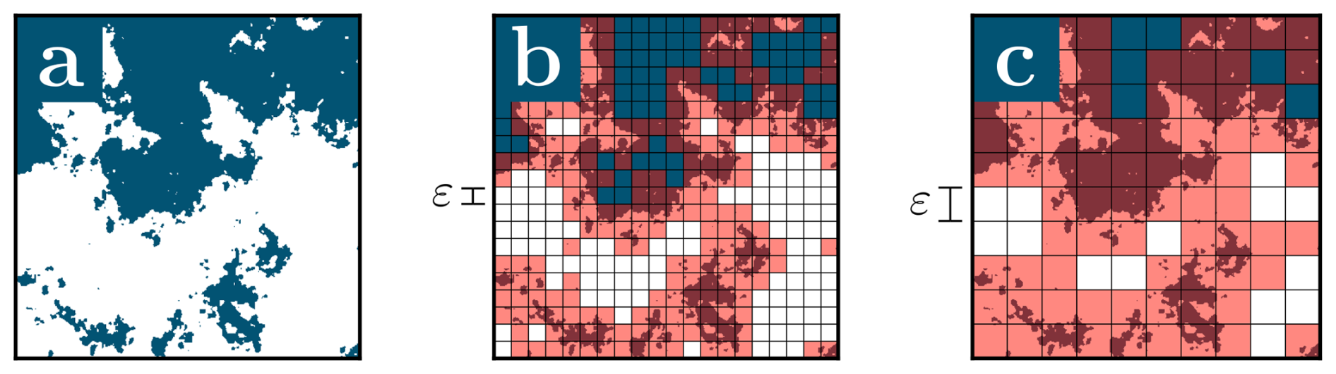
Figure 8 Calculation of the box dimension from a binary cloud mask (a). A grid with varying box size ε is overlaid on the cloud mask (b, c) such that each box contains ε×ε image pixels. Here, ε=25 for panel (b) and ε=50 for panel (c). The number of boxes required to cover all cloud edges (marked in red) is counted as a function of ε to obtain N(ε).

Although the actual resolution of the cloud mask ξ is fixed, the box size ε serves as an effective resolution for the purpose of calculating the fractal dimension as defined by Mandelbrot, equivalent in the limit ε→0 to that definition given by Eqs. (1) or (5) since $P\sim \mathit{\epsilon }N\sim {\mathit{\epsilon }}^{\mathrm{1}-D_{\text{box}}}$. There are, however, two other limiting cases. For a cloud field resolved at some finite resolution ξ, the box dimension D_box will tend to unity if the box length is smaller than the satellite resolution, that is ε≲ξ. This is because D_box will correspond to the Euclidean dimension of a line, in this case a pixel edge. Similarly, for boxes larger than the domain D_box=0 because a single box is always sufficient to cover all cloud edges, implying N(ε) is independent of ε for such large boxes.

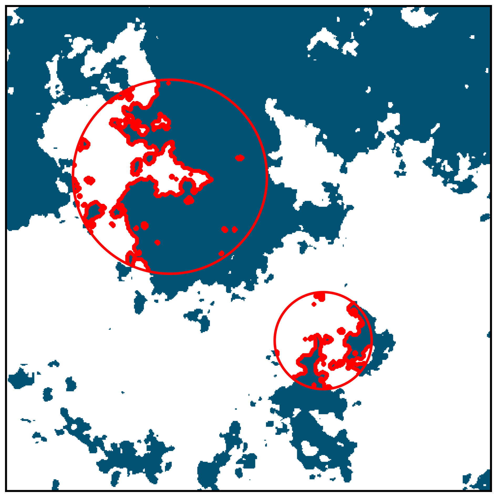
Figure 9 Example calculation of the correlation dimension. The red circles are centered at two randomly selected cloud edge pixels. For each circle center j, a component of the correlation integral C_j is calculated by counting the number of cloud edge pixels (red) within the circle as a function of circle radius r.

A second approach commonly used to measure the fractal dimension is the “correlation integral” method (Grassberger and Procaccia, 1983). For clouds, this consists of first identifying all cloud edge pixels (i.e. cloudy pixels that are adjacent to a clear pixel). For each pixel with index j, a circle of varying radius r is drawn centered on that pixel (Fig. 9). The total number of cloud edge pixels within the circle C_j(r) is computed as a function of r. The fractal dimension is then calculated using the “correlation integral” $C\left(r\right)={\sum }_j{C}_j\left(r\right)$, which tends to be a power law of form

$$\begin{array}{}\text{(9)}& C\left(r\right)\propto r^{D_{\mathrm{c}}}\end{array}$$

where D_c is the “correlation dimension”. Although not strictly equivalent to Mandelbrot's ensemble fractal dimension (Eq. 5), D_c is empirically very close to D_e (Strogatz, 2018), perhaps unsurprisingly given that both represent a relationship between the scale under consideration (represented by ε or r) and the density of cloud edge points (represented by N(ε) or C(r)). In practice, C(r) follows a power law only for a finite range in r. As with the box dimension, the correlation dimension tends toward the Euclidean dimensions of a single pixel for small r and the domain shape for large r. Accordingly, below we will only consider circles with r≥3ξ.

An important subtlety for calculation of D_c is that, without proper care, some circles might extend beyond the domain boundary. If C_j(r) is computed including such circles, D_c can become biased towards the dimension of the artificially straight domain boundary of D_c=1 at large scales. To remedy this issue, here we ensure that no circles extend beyond the domain boundary by enforcing $r\le r_{\text{max}}=\text{min}(L,W)/\mathrm{3}$ where W and L are the domain width and length, respectively. We then only draw circles when the distance between the circle center and the nearest domain edge point is at least r_max. Note that including contributions from small circles that are closer to the domain edge than r_max, even when they do not extend beyond the domain edge, can still introduce boundary artifacts. This is because a set of values for C_j(r) that contained data only from small circles would bias the sum C(r) to be too large for small r.

There is a statistical advantage of using the correlation dimension for analysis of cloud fields, which is that C(r) is created using a much greater number of measured values compared with N(ε). This is because C(r) is a sum over many circle center locations j located along cloud edge – even for a single cloud. Accordingly, the correlation dimension is better suited for satellite datasets with fewer clouds or those obtained at coarse resolution.

4.3 Measurements

For the box dimension, Fig. 10 shows the number of cloud edge boxes N as a function of box length ε for all 72 MODIS images and six reflectance thresholds R as described in Sect. 2. As expected, D_box≈1 for boxes that are small compared to the satellite resolution, and D_box=0 for very large boxes comparable to the domain size. For intermediate sized boxes, D_box varies from $D_{\text{box}}=\mathrm{1.68}\pm \mathrm{0.05}$ for threshold R=0.1 to $D_{\text{box}}=\mathrm{1.50}\pm \mathrm{0.07}$ for R=0.35 suggesting (plausibly) that the more reflective regions of clouds are some combination of either being more often large, with smaller β, or more Euclidean, with smaller D_i.

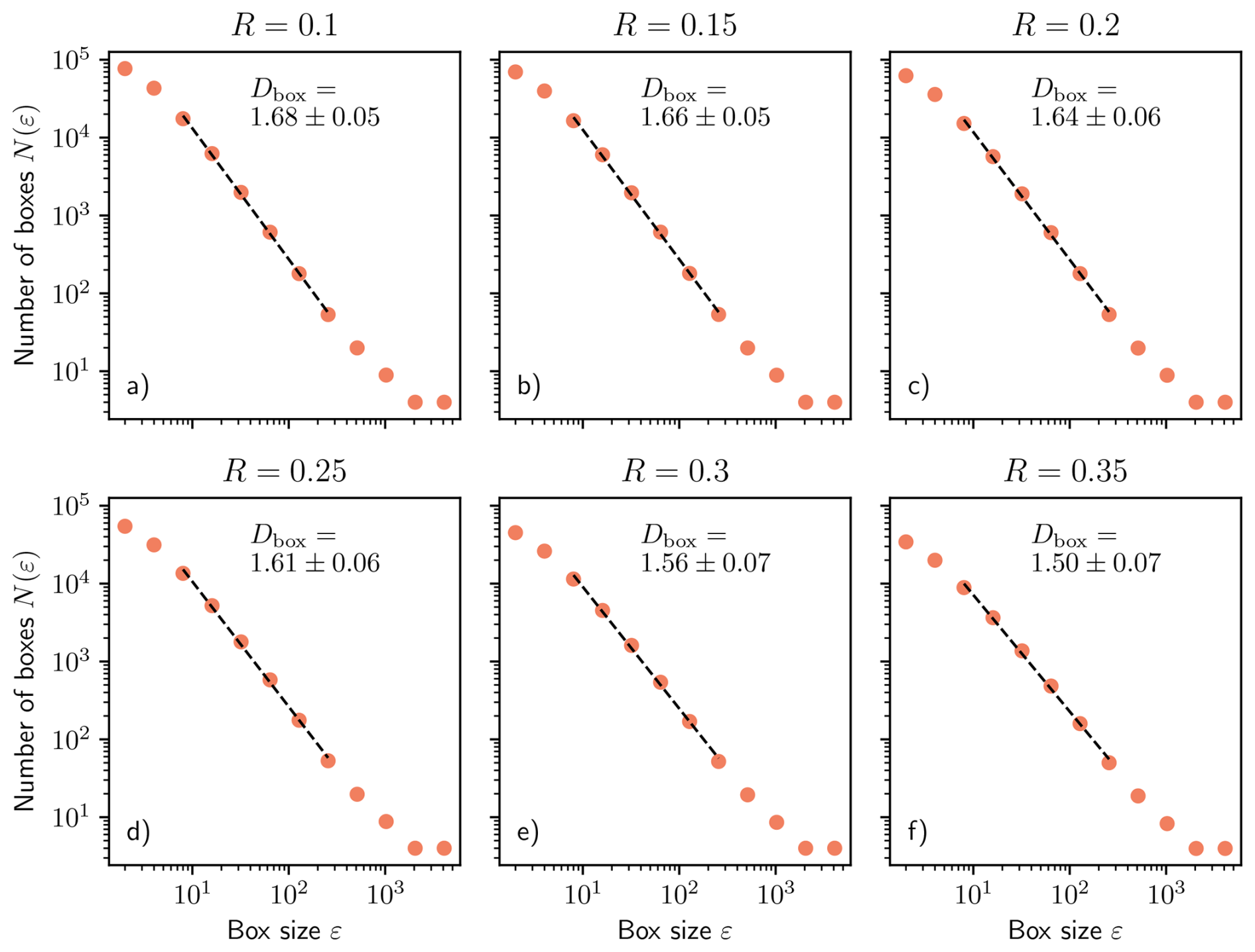
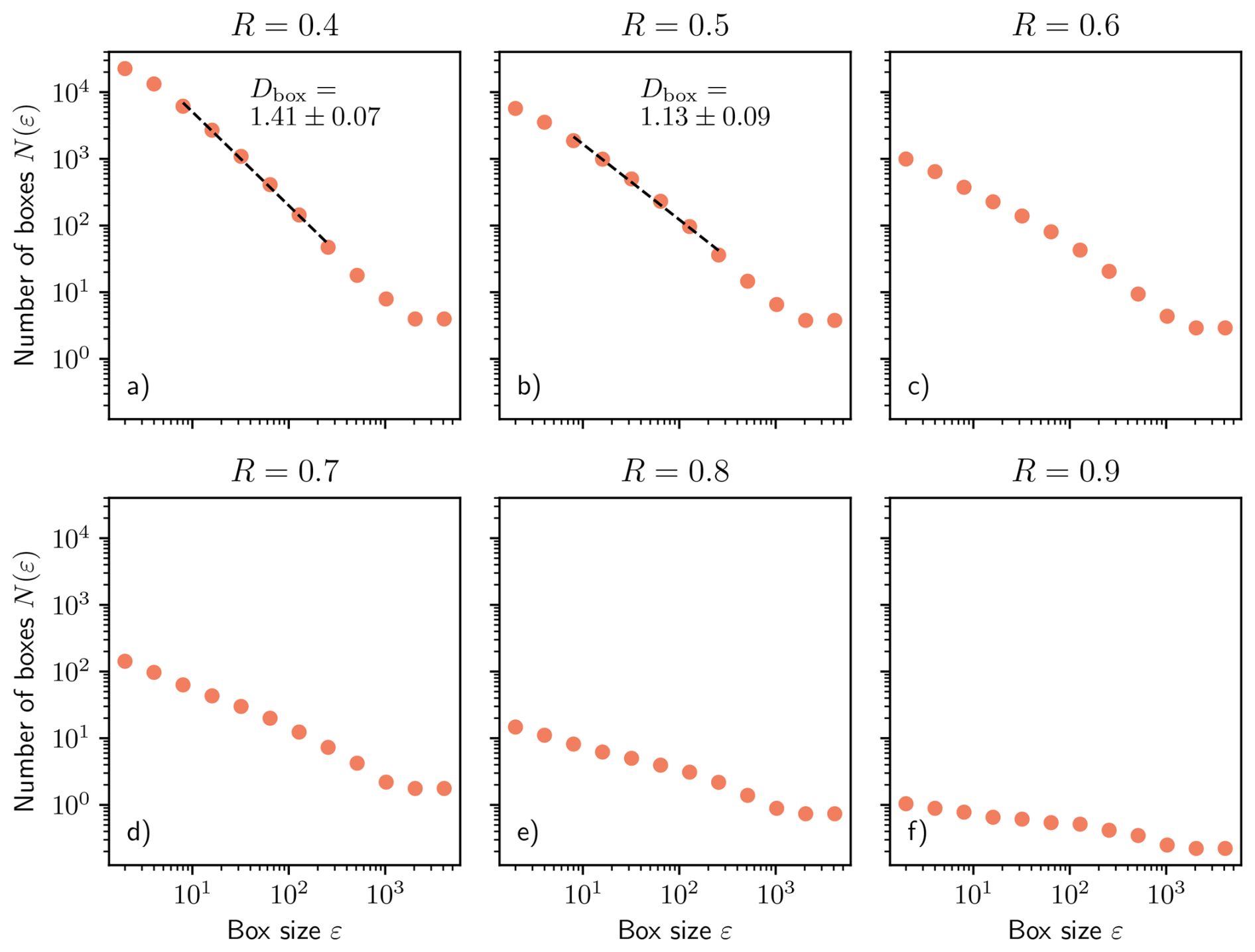
Figure 10 Measurements of the ensemble fractal dimension D_e (Eq. 5) using the box dimension $N\left(\mathit{\epsilon }\right)\propto {\mathit{\epsilon }}^{-D_{\text{box}}}$, where N is the number of boxes of side length ε required to cover all cloud perimeters (Fig. 8). At small and large ε, D_box tends toward the values of a pixel (D_box=1) or a point (D_box=0), respectively. The box dimension attains a roughly constant intermediate value for medium-sized boxes, corresponding to the ensemble fractal dimension D_e.

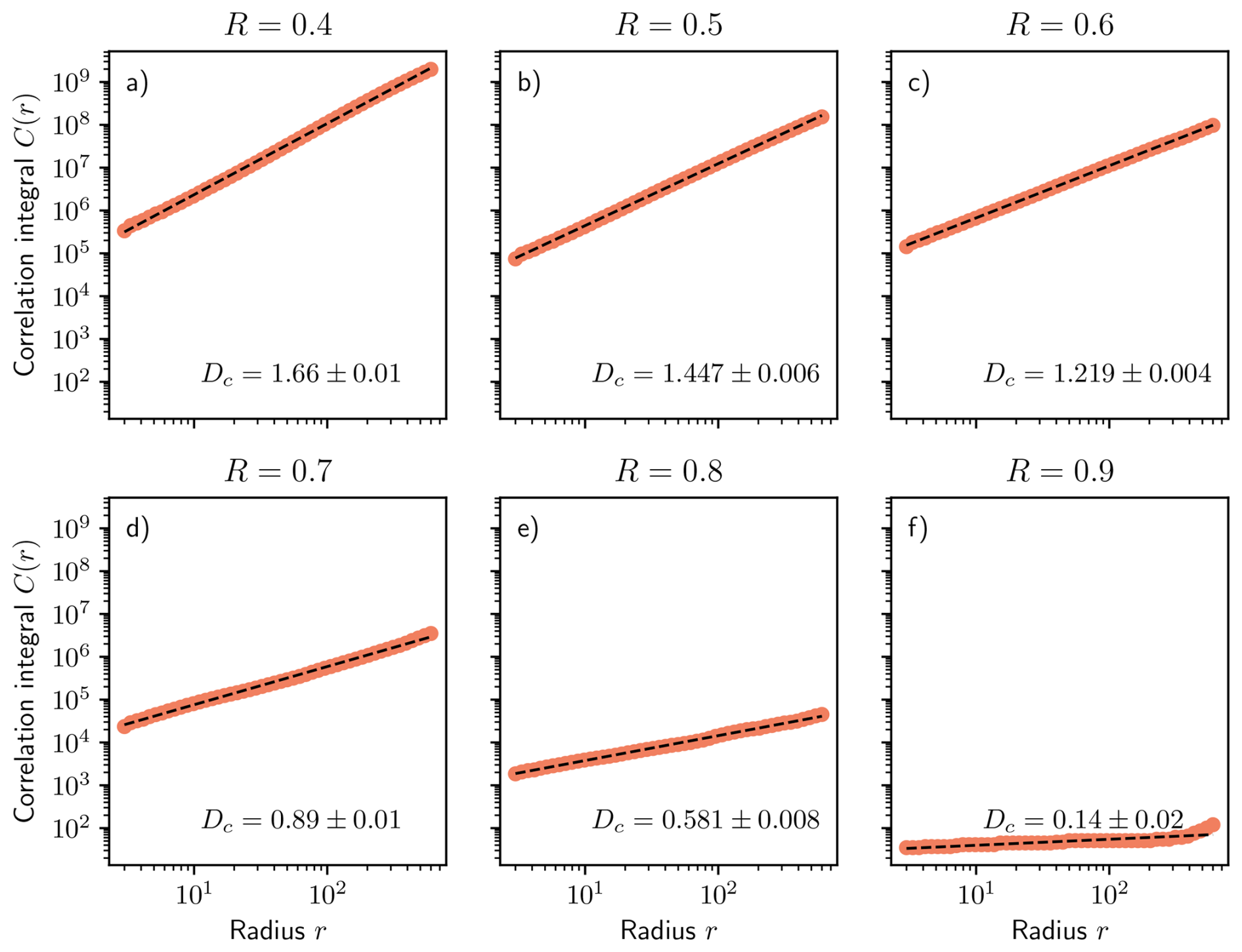
For the correlation dimension, we find that observed values of C(r) for clouds scale with r, implying a measured correlation dimension for the cloud field ranging from 1.77±0.01 for a reflectance threshold of R=0.1 to 1.69±0.01 for R=0.35 (Fig. 11). These values are somewhat higher than those obtained using the box dimension but display a similar trend of decreasing values with increasing R. As shown in Fig. 11, the correlation integral C(r) is better represented by a power-law when compared to the box-counting function N(ε) (Fig. 10), implying estimates of D_c are more accurate when compared to D_box.

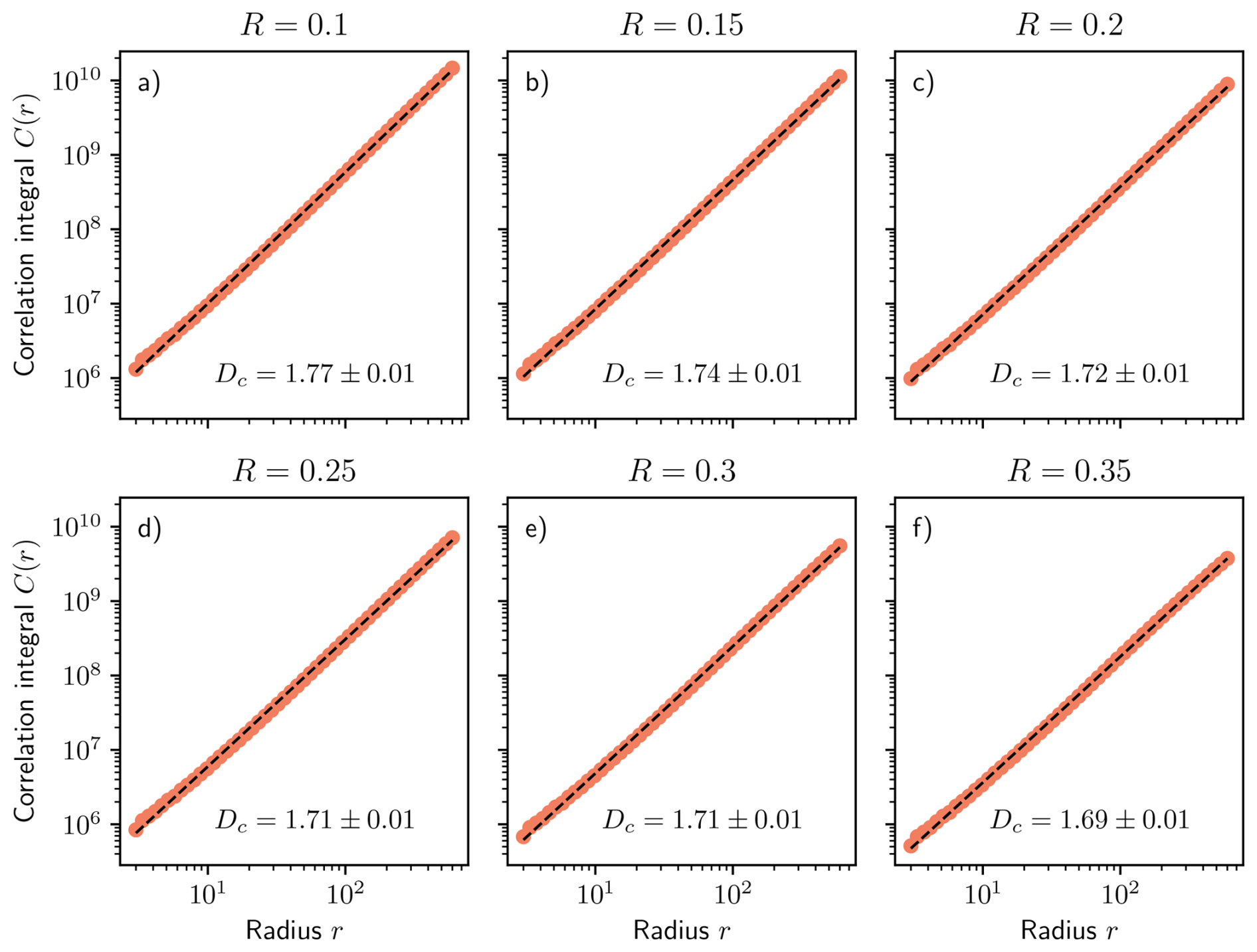
Figure 11 Measurements of the ensemble fractal dimension D_e (Eq. 5) using the correlation dimension, defined by $C\left(r\right)\propto r^{D_{\mathrm{c}}}$, for the MODIS cloud ensemble for a selection of reflectivity thresholds R defining cloud.

To evaluate the hypothesis that D_e=βD_i (Eq. 7), β is determined directly from the MODIS cloud masks. Accurately determining the power-law distribution exponent in satellite data can be surprisingly challenging, primarily because the artificial truncation of clouds along the domain edge can influence the measured cloud size distribution. A comprehensive analysis of the possible biases arising from domain truncation was done by DeWitt and Garrett (2024). Here, we implement their recommended methodology, which was to calculate β using a linear regression to a logarithmically binned and transformed histogram of cloud perimeter (Fig. 12). As recommended by DeWitt and Garrett (2024), fits are performed only for those bins for which at least 50 % of clouds in that bin are entirely contained within the measurement domain. This method ensures that β is calculated from only the unbiased portion of the distribution, i.e. the portion that is not dominated by large clouds that extend beyond the measurement domain. This filtering removes approximately 0.06 % to 0.4 % of all clouds depending on threshold.

Figure 12 Distributions of cloud perimeters used to calculate the power-law distribution exponent β (Eq. 6). Fitted values of β are reported in Table 1.

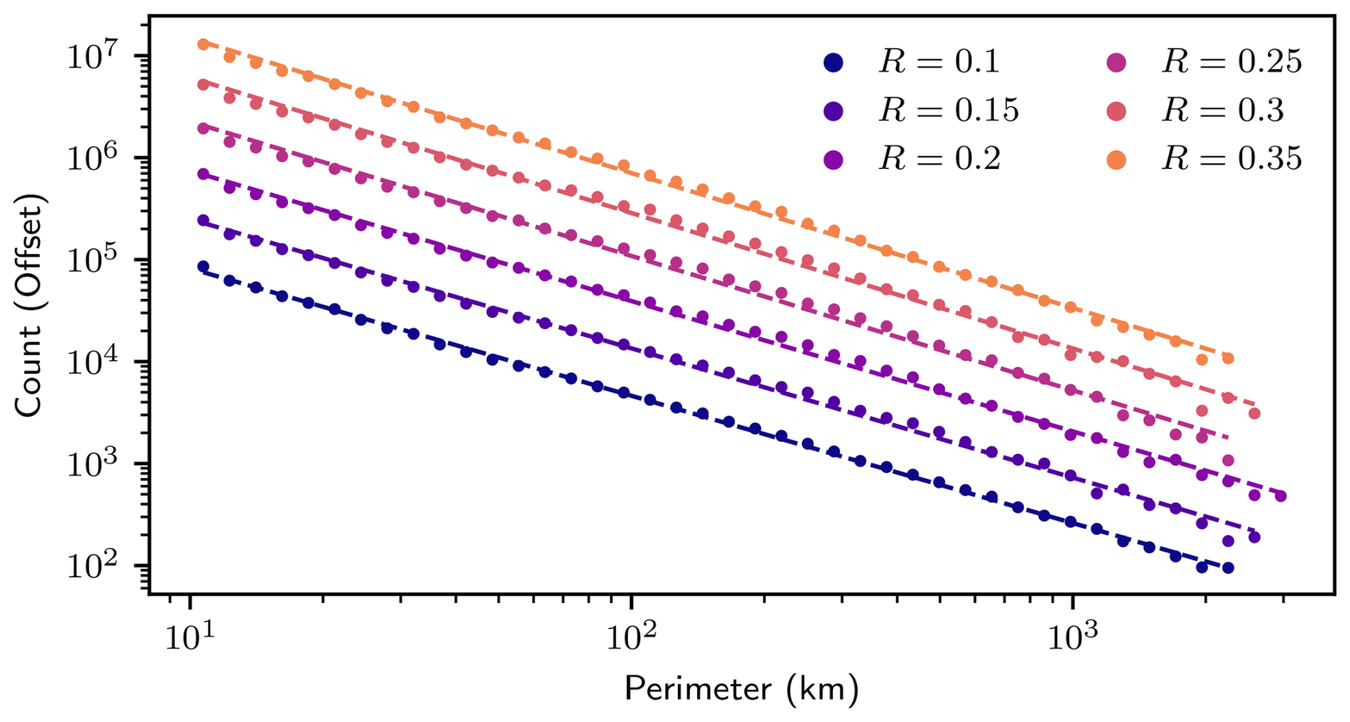
Another consideration for the calculation of β is the presence of “nested perimeters” (Appendix B), or the perimeters of cloud holes and even nested clouds within cloud holes. Here, we take the approach that each nested perimeter is in effect a distinct cloud edge, for which there is a distinct value to be considered in the power law fit used to determine a value for β (Garrett et al., 2018). In effect, a single cloud may possess multiple perimeter values if it contains holes. The alternative approach would be to sum the exterior perimeter of a cloud with the perimeter of all the holes within the cloud prior to fitting. Appendix B considers this distinction further and shows that the method employed here of including nested perimeters results in values of β that are larger by approximately 0.1.

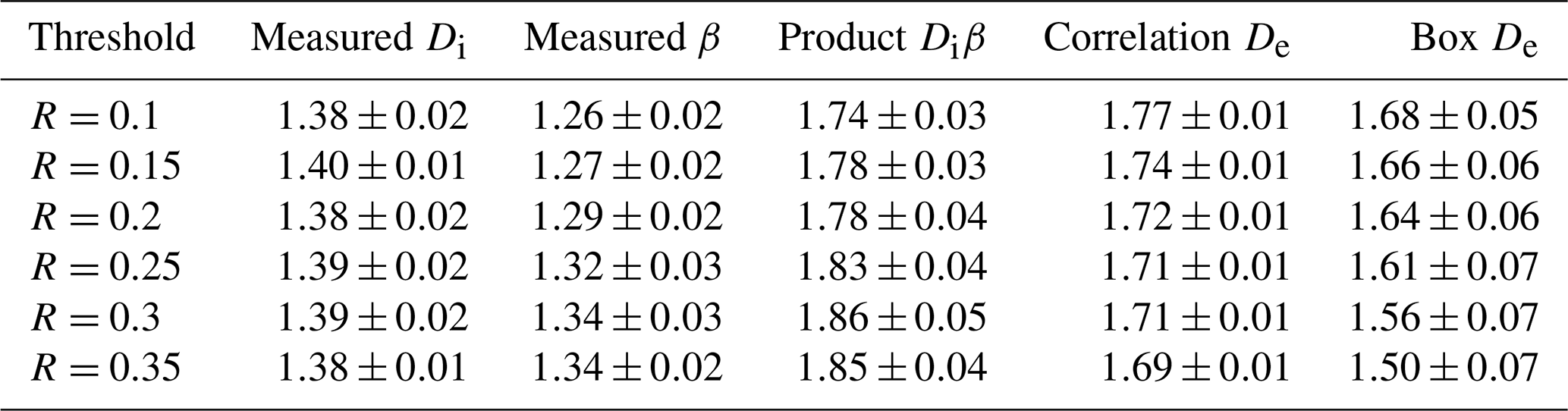
Table 1 compares the calculated values of the box dimension and correlation dimension to the product βD_i. Generally, the fractal dimension decreases with threshold R, although the dependence is significant only for D_e with minimal sensitivity for D_i (see Appendix C for values of D_e calculated using a wider range of thresholds). Such dependence is an indication that cloud fields are “multifractal”, a term meaning that the ensemble fractal dimension is a function of the thresholding scheme used to binarize the cloud field. Such multifractal behavior has been used to shed light on turbulent intermittency in the atmosphere and indicates that the intensity of the turbulence varies spatially (Lovejoy and Schertzer, 1990).

As shown in Table 1, all three methods for calculating the ensemble fractal dimension – the box dimension, correlation dimension, and βD_i – point to a value roughly between 1.6 and 1.8, with a possible exception of the box dimension at higher reflectivity thresholds. Although D_c and D_box decrease with increasing threshold, the product βD_i displays less of a trend due to the relatively weak dependence of both β and D_i on R. More importantly, whichever method is used to calculate D_e, the values are substantially higher than those for the individual fractal dimension D_i, which has a value of approximately 1.4 (Fig. 6).

Table 1 Comparison of the individual fractal dimension D_i with the three methods of calculating the ensemble fractal dimension D_e: the box dimension, correlation dimension, and the product D_e=βD_i (Eq. 7).

For cloud fields, this distinction between the two fractal dimensions D_i and D_e has been almost entirely overlooked by previous studies, most of which only considered D_i (Lovejoy, 1982; Henderson-Sellers, 1986; Bazell and Desert, 1988; Gifford, 1989; Cahalan and Joseph, 1989; Jayanthi et al., 1990; Sengupta et al., 1990; Chatterjee et al., 1994; Gotoh and Fujii, 1998; Siebesma and Jonker, 2000; Luo and Liu, 2007; Peters et al., 2009; von Savigny et al., 2011; Brinkhoff et al., 2015; Batista-Tomás et al., 2016; Christensen and Driver, 2021; Janssens et al., 2021; Cheraghalizadeh et al., 2024). The few studies that measured D_e did so by box-counting (Lovejoy et al., 1987; Carvalho and Dias, 1998; Janssens et al., 2021) but without noting that D_i and D_e are different. Conflating the two different dimensions could lend a false impression of a discrepancy between studies, when in reality the two values simply reflect the difference between the geometries of individual clouds and those of a cloud field.

5 Conclusions

There is a need to validate numerical simulations of cloud sizes, shapes, and organization through comparisons with observations. Subjective classification schemes exist (Stevens et al., 2020), but objective mathematical metrics offer distinct advantages, especially when they can be related directly to underlying physical processes such as symmetry principles and can be applied uniformly across a wide range of spatial scales. Here, we explored the suitability of two metrics focused on the geometries of cloud edges: the individual fractal dimension D_i that characterizes the geometric complexity of individual clouds, and an ensemble fractal dimension D_e that captures how the cloud field organizes hierarchically into structures spanning a wide range of sizes and shapes. A Python package that implements the recommended methodology is made available (DeWitt, 2025). Although both fractal dimensions have been previously studied, the distinction has not been widely discussed. The satellite observations of cloud fields we present here show a significant quantitative difference, with D_i≈1.4 and D_e≈1.7. We propose and observationally test that the two quantities can be related through the exponent β for a power-law fit to the number distribution of cloud perimeters in the cloud field, namely D_e=D_iβ.

By strict definition, the individual fractal dimension D_i is determined from the resolution dependence of the perimeter of an individual cloud. Because satellites have fixed resolution, the more common technique is to consider a cloud ensemble and to fit the logarithm of cloud perimeter to the logarithm of cloud area. We show that this approach is fraught because clouds have holes. Not filling cloud holes violates the strict definition of the fractal dimension, while filling the holes misses an important physical property defining the cloud field.

Calculation of the ensemble fractal dimension D_e bypasses these issues and may offer a more objective alternative to a subjective classification scheme such as sugar, gravel, fish, and flowers (Stevens et al., 2020), particularly if calculated as a correlation integral. The ease of its calculation using the correlation integral in satellite imagery makes it well-suited for future evaluations of the accuracy of atmospheric numerical simulations or for comparing regional meteorology. D_e also has the potential to identify fundamental physical differences in atmospheric states relating to their scaling symmetries as it has been linked to the otherwise invisible and complex turbulent processes that shape cloud edge (Hentschel and Procaccia, 1984; Lovejoy et al., 1987; Siebesma and Jonker, 2000; Rees et al., 2024).

Although understanding clouds as objects might seem simple and intuitive at first, the hidden subtleties identified here prove surprisingly problematic, raising questions for future work. It is perhaps noteworthy that we tend to map a continuous reflectance field onto discrete entities called clouds, but that we do not do so for other continuous fields such as wind and temperature. One might reasonably wonder whether the subtleties described here are worth the care required, or whether some continuous field-based approaches might ultimately prove superior (Lovejoy and Schertzer, 2010).

Appendix A: The relationship between the individual and ensemble fractal dimension

Here we derive Eqs. (5) and (7), showing the link between the ensemble property P and the individual cloud property D_i. Conceptually, as illustrated in Fig. A1, there are two factors that lead to P changing as the measurement resolution is varied. The first relates to the fractal dimension for individual clouds D_i (Eq. 1). The second relates to the minimum resolved size of a feature. This changes not the total number of clouds considered, but more strictly the number of closed contours defining cloud edges. A closed contour could be defined by first starting at one cloud edge point and following the boundary between cloudy and clear sky until the original point is reached. Any given cloud's boundary may be broken into multiple closed contours if the cloud contains holes – one corresponding to its exterior edge and one for each hole.¹

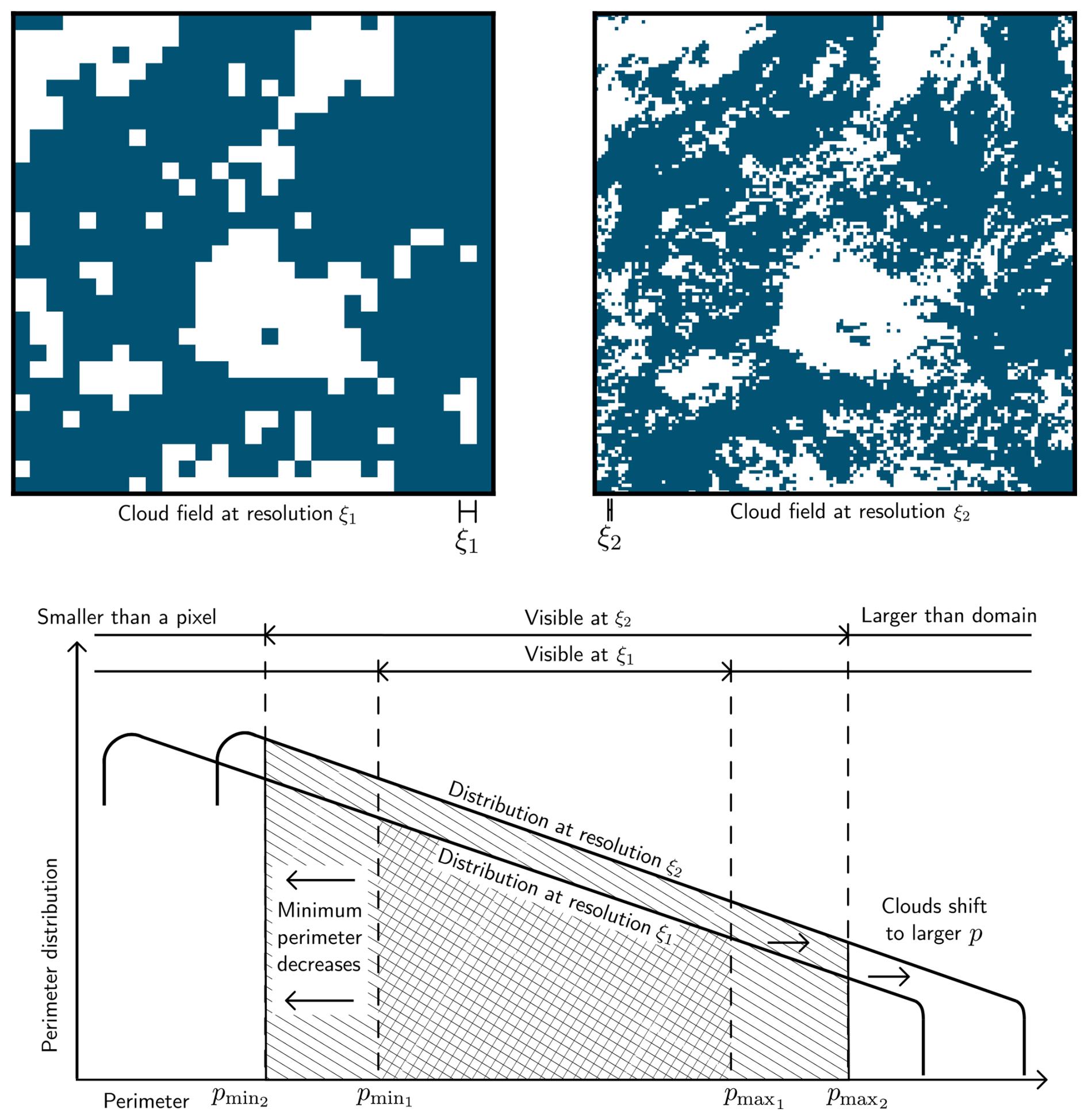
Figure A1 Cartoon of the changes to the logarithmically-scaled perimeter density (bottom) corresponding to a hypothetical rescaling from a resolution ξ₁ to a finer resolution ξ₂, i.e. ξ₁>ξ₂ (top). The figure depicts the two effects to the total number of clouds as the resolution changes. The total number of clouds at ξ₁ (cross-hatched area) is smaller than the total number measured at ξ₂ (single-hatched plus cross-hatched area) for two reasons: first, the $p_{{\text{min}}_{\mathrm{2}}}<p_{{\text{min}}_{\mathrm{1}}}$, which adds the hatched area on the left. Second, the distribution for ξ₁ becomes, due to its rightward shift, vertically offset from the distribution at ξ₂, which adds the hatched area at the top. Note that, due to the logarithmic scale, the added area on the right caused by an increase in $p_{{\text{max}}_{\mathrm{2}}}>p_{{\text{max}}_{\mathrm{1}}}$ is negligible.

The relative contribution of small perimeters to the total is determined by the normalized size distribution of cloud perimeters, which from Eq. (6) follows

$$\begin{array}{}\text{(A1)}& {\displaystyle }\begin{array}{rl}& n\left(p\right)\equiv {\displaystyle \frac{\mathrm{d}n}{\mathrm{d}p}}=n_{\mathrm{0}}{p}^{-(\mathit{\beta }+\mathrm{1})},\\ & p_{\text{min}}<p<p_{\text{max}},\mathit{\beta }>\mathrm{0},\end{array}\text{(A2)}& {\displaystyle }{n}_{\mathrm{0}}={\displaystyle \frac{\mathit{\beta }}{p_{\text{min}}^{-\mathit{\beta }}-p_{\text{max}}^{-\mathit{\beta }}}},\end{array}$$

where n₀ is a normalization constant and p_min and p_max represent the smallest and largest measurable perimeters, respectively. The total perimeter P is the mean cloud perimeter ${\int }_{p_{\text{min}}}^{p_{\text{max}}}pn\left(p\right)\mathrm{d}p$ multiplied by the total number of clouds N:

$$\begin{array}{}\text{(A3)}& {\displaystyle }P=N\underset{p_{\text{min}}}{\overset{p_{\text{max}}}{\int }}pn\left(p\right)\mathrm{d}p.\end{array}$$

Satellite observations show β≈1.26 (DeWitt et al., 2024). Given that β≠1 the integral in Eq. (A3) may be calculated:

$$\begin{array}{}\text{(A4)}& {\displaystyle }P{\displaystyle }=N{\displaystyle \frac{\mathit{\beta }}{\mathit{\beta }-\mathrm{1}}}\left({\displaystyle \frac{p_{\text{min}}^{\mathrm{1}-\mathit{\beta }}-p_{\text{max}}^{\mathrm{1}-\mathit{\beta }}}{p_{\text{min}}^{-\mathit{\beta }}-p_{\text{max}}^{-\mathit{\beta }}}}\right),\mathit{\beta }\ne \mathrm{1}.\end{array}$$

We may now make several simplifications. The first is that the terms involving p_max may be dropped since $p_{\text{max}}^{\mathrm{1}-\mathit{\beta }}\ll p_{\text{min}}^{\mathrm{1}-\mathit{\beta }}$, as previously observed to frequently hold (DeWitt et al., 2024). Additionally, we can replace p_min with the resolution ξ times some constant c. This is because the minimum possible measurable cloud size is determined by the resolution – for example, if single-pixel clouds are counted towards the total perimeter then p_min=4ξ. With these simplifications,

$$\begin{array}{}\text{(A5)}& {\displaystyle }P{\displaystyle }=N{\displaystyle \frac{\mathit{\beta }c}{\mathit{\beta }-\mathrm{1}}}\mathit{\xi },\mathit{\beta }>\mathrm{1},p_{\text{max}}\gg p_{\text{min}}.\end{array}$$

The next step is to calculate the resolution dependence of N, the total number of clouds. As shown in Fig. A1, N can be conceptualized as the area under the curve of n(p), and as the resolution changes, this area changes in two orthogonal ways: first, the enclosed area grows or shrinks horizontally (the p direction in Fig. A1) due to changes in p_min, and second, the distribution itself moves in p, n(p)-space as each cloud's perimeter coordinate changes via Eq. (1), resulting in a vertical change in the area under n(p).

Expressed logarithmically, the two effects are, respectively,

$$\begin{array}{}\text{(A6)}& {\displaystyle \frac{\mathrm{d}\ln N}{\mathrm{d}\ln \mathit{\xi }}}={\displaystyle \frac{\partial \ln N}{\partial \ln \mathit{\xi }}}{|}_{n\left(p\right)}+{\displaystyle \frac{\partial \ln N}{\partial \ln \mathit{\xi }}}{|}_{p_{\text{min}}}.\end{array}$$

For the first term, n(p) is constant with respect to ξ (Eq. A1). Integrating Eq. (A1) from an arbitrary minimum perimeter cξ to p_max and again approximating p_max→∞, we have $N\propto {\mathit{\xi }}^{-\mathit{\beta }}$ or

$$\begin{array}{}\text{(A7)}& {\displaystyle \frac{\partial \ln N}{\partial \ln \mathit{\xi }}}{|}_{n\left(p\right)}=-\mathit{\beta }.\end{array}$$

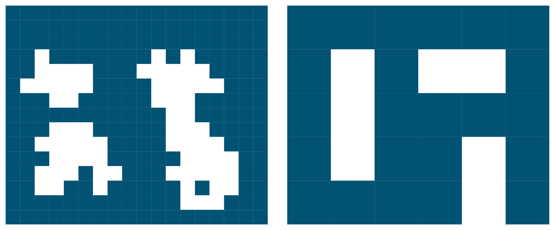
Figure A2 Conceptual example of how clouds could appear to break apart or combine as the resolution ξ changes. Here, the right image is coarsened by averaging, for each pixel, the corresponding 3×3 pixel region in the left image and then rounding values to 1 (white) or 0 (blue). On the left side of the image, clouds appear to merge as the resolution is coarsened, while on the right, the opposite occurs. The ensemble fractal dimension is derived by neglecting the net effect of cloud merging or breaking apart.

The second term in Eq. (A6) represents the distribution itself shifting in perimeter space, and is in effect an “advection” equation analogous to a conservation law, but with “advection” here representing the change to each cloud's perimeter in perimeter space, not a change to the cloud's location in physical space. Expressed logarithmically, the advection equation is

$$\begin{array}{}\text{(A8)}& {\displaystyle \frac{\partial \ln N}{\partial \ln \mathit{\xi }}}{|}_{p_{\text{min}}}=-{\displaystyle \frac{\partial \ln p}{\partial \ln \mathit{\xi }}}{\displaystyle \frac{\partial \ln N}{\partial \ln p}}.\end{array}$$

Notably, Eq. (A8) assumes cloud number is locally conserved. As an example, Fig. A2 shows how this assumption could conceivably be violated: as the resolution changes, clouds could appear to combine or break apart, thereby changing the number of clouds. We neglect these effects with the justification that any reduction in cloud number due to clouds combining might easily be offset by clouds breaking apart (as in the example in Fig. A2), limiting any net change in cloud number.

From the integrated form of Eq. (A1), N is proportional to p^−β, which implies that $\partial \ln N/\partial \ln p=-\mathit{\beta }$. Additionally, Eq. (1) implies that $\partial \ln p/\partial \ln \mathit{\xi }=\mathrm{1}-D_{\mathrm{i}}$, so

$$\begin{array}{}\text{(A9)}& {\displaystyle \frac{\partial \ln N}{\partial \ln \mathit{\xi }}}{|}_{p_{\text{min}}}=\mathit{\beta }-\mathit{\beta }{D}_{\mathrm{i}}.\end{array}$$

Substituting Eqs. (A9) and (A7) into Eq. (A6) we obtain

$$\begin{array}{}\text{(A10)}& {\displaystyle \frac{\mathrm{d}\ln N}{\mathrm{d}\ln \mathit{\xi }}}=-\mathit{\beta }{D}_{\mathrm{i}}\end{array}$$

and, from Eq. (A5), the total perimeter P is given by

$$\begin{array}{}\text{(A11)}& {\displaystyle }P\left(\mathit{\xi }\right)\propto {\mathit{\xi }}^{\mathrm{1}-\mathit{\beta }{D}_{\mathrm{i}}},\mathit{\beta }>\mathrm{1}.\end{array}$$

If we define D_e=βD_i as in Eq. (7), we obtain Eq. (5), consistent with Mandelbrot's assumption of a power law for P.

The case of β equaling unity

While $\mathit{\beta }\approx \mathrm{1.26}>\mathrm{1}$ has been observed to apply to satellite images of cloud perimeters that are seen from above (DeWitt et al., 2024), the case of β≈1 is also physically realistic for the case that perimeters are measured within thin horizontal layers (Garrett et al., 2018), as is possible in a numerical simulation.

In place of Eq. (A4), the total perimeter formula becomes

$$\begin{array}{}\text{(A12)}& {\displaystyle }P=N{p}_{\text{min}}\ln \left({\displaystyle \frac{p_{\text{max}}}{p_{\text{min}}}}\right),\mathit{\beta }=\mathrm{1}.\end{array}$$

where, again, p_min=cξ with c a constant. In this case, the contribution of large clouds toward P cannot be neglected. Instead, we can use Eq. (1) to obtain $p_{\text{max}}=b{\mathit{\xi }}^{\mathrm{1}-D_{\mathrm{i}}}$ with b some large constant that increases with domain area. From Eqs. (A10) and (A12) we have

$$\begin{array}{}\text{(A13)}& {\displaystyle }P\propto {\mathit{\xi }}^{\mathrm{1}-D_{\mathrm{i}}}\ln \left({\displaystyle \frac{b}{c{\mathit{\xi }}^{D_{\mathrm{i}}}}}\right),\mathit{\beta }=\mathrm{1}\end{array}$$

In this case, P(ξ) no longer exhibits a pure power law dependence on ξ because there is an additional logarithmic factor. However, if b≫c, roughly corresponding to p_max≫p_min, the logarithmic term is a slowly-varying function of ξ for realistic values of p_max and p_min determined using the MODIS observations described in Sect. 4.3 (not shown). In this case, P(ξ) might be approximated by the power law $P\propto {\mathit{\xi }}^{\mathrm{1}-D_{\mathrm{i}}}$ over a limited range of measurement resolutions. It is therefore conceivable that the equation D_e=βD_i (Eq. 7) may still apply for β=1, although further work is needed to determine if this is indeed the case.

Appendix B: Comparison of the perimeter distribution exponent with and without cloud holes

When calculating distributions for cloud perimeters, there is ambiguity about how to treat clouds with holes. On the one hand, prior to calculating distribution parameters, the perimeter of any holes within a given cloud might be summed with the exterior perimeter of the cloud, a method we term “summed values”. Alternatively, each individual boundary might be considered as contributing a unique perimeter value to the histogram from which the distribution exponent β is calculated. This method, which we term “nested values”, was used in Sect. 4.3. For example, a doughnut-shaped cloud would have a single value for its perimeter for the summed case but two values for the nested case, one corresponding to the hole's perimeter and one to the exterior perimeter.

Table B1 compares the sensitivity of calculations of β (Eq. 6) to whether the summed or nested values approach is taken. For all considered thresholds in reflectivity R, β is larger if the nested value method is used. This is for two reasons. First, adding hole perimeter to a cloud's exterior perimeter increases that cloud's perimeter, placing it in a larger bin. Second, summing reduces the number of perimeters in a smaller bin because the hole perimeters are no longer counted in the smaller bin. Both effects act to decrease the slope of the distribution, making β smaller, even as both cases produce size distributions that are well-described by a power law distribution (Fig. B1).

Given that cloud holes do exist, and that they are not considered for D_i, we employ the “nested” methodology in the main text as it more realistically represents the role of cloud holes.

Table B1 Comparison of calculated values of β for two methods of treating cloud holes as a function of reflectance threshold R. Histograms from which values for β are calculated are shown in Fig. B1. Values for β are only calculated when the distribution spans two orders of magnitude (Stumpf and Porter, 2012) after bins containing less than 30 counts are removed (DeWitt and Garrett, 2024).

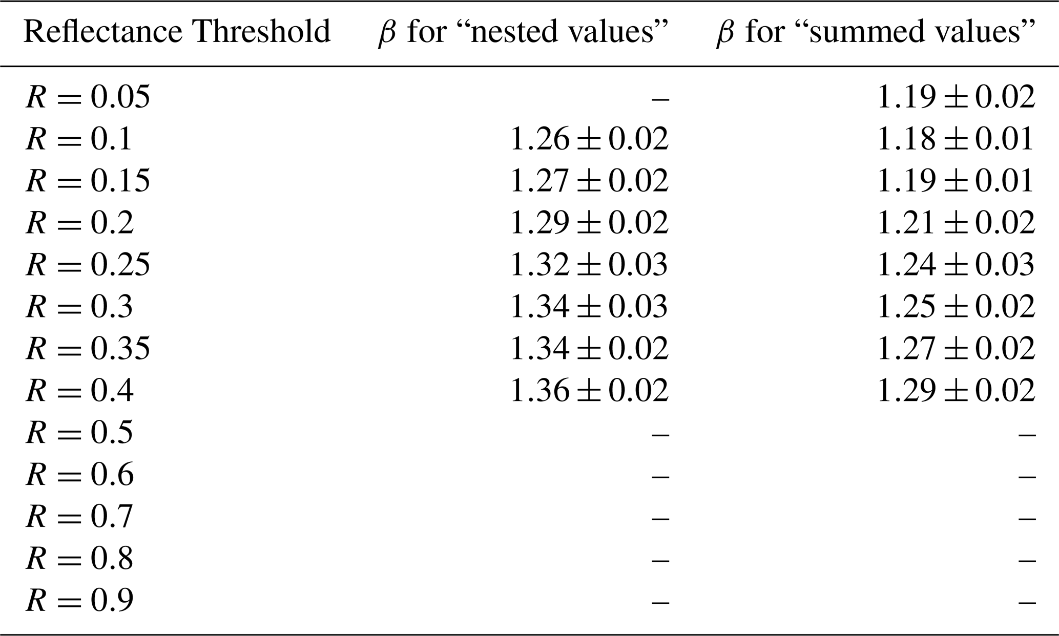
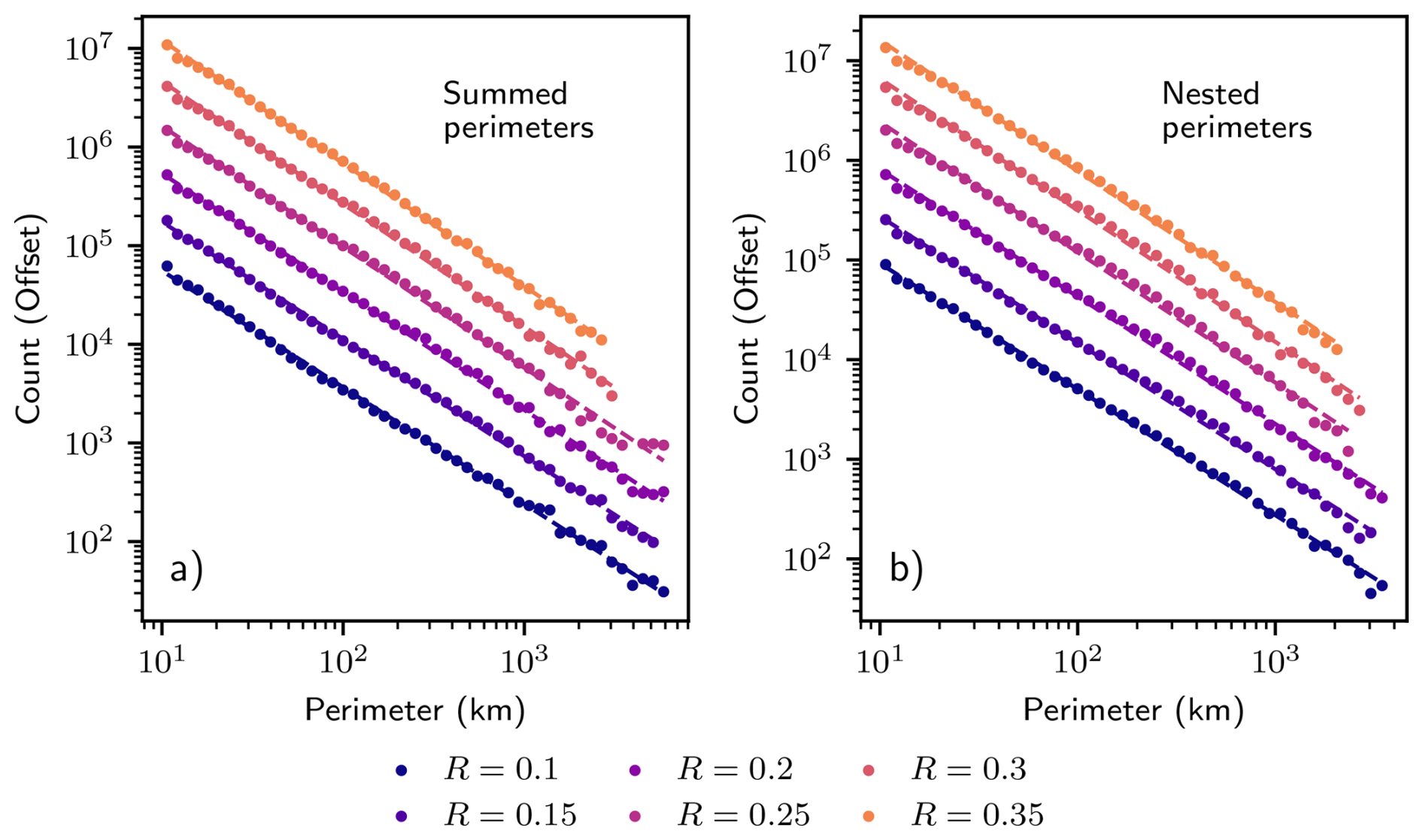
Figure B1 Histogram of cloud perimeters for various thresholds in reflectance R, calculated for both cases described in the text. Counts for thresholds larger than R=0.1 are vertically offset by factors of 3 for clarity. Values and uncertainties for the slopes, which correspond to −β (Eq. A1), are listed in Table B1. Perimeter values smaller than 10 km, bins with counts smaller than 30, or bins in which a majority of clouds extend beyond the measurement domain are omitted from the plot and regression (DeWitt and Garrett, 2024).

Appendix C: Parameters for a wider range of reflectance thresholds

In the main text, reflectance thresholds R used to define cloud were limited to a range between R=0.1 to R=0.35. The reason is that higher thresholds reduce the number of clouds and therefore the statistical robustness of the results. Additional thresholds, at which only some parameters can be reliably estimated, are listed in Table C1. Figures C1, C2, and C3 are as in Figs. 6, 10, and 11 but for these additional reflectance thresholds.

Table C1 As in Table 1, but for a wider range of reflectance thresholds R. Values for β are only calculated when the distribution spans two orders of magnitude (Stumpf and Porter, 2012) after bins containing less than 30 counts are removed (DeWitt and Garrett, 2024). Likewise, values for D_i are only listed when $\sqrt{a_{\mathrm{f}}}$ spans at least two orders of magnitude, and the box and correlation dimensions are only calculated when C(r)>30 and N(ε)>30 for all r and ε, respectively.

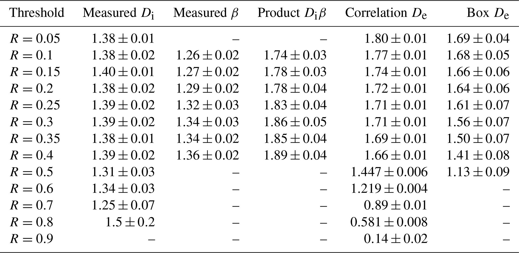
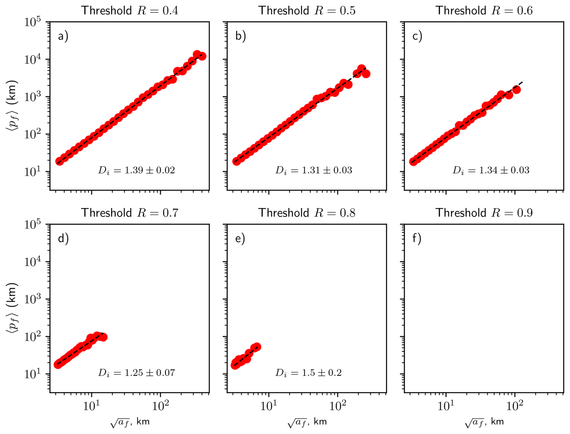
Figure C1 As in Fig. 6, but for larger reflectance thresholds R. Threshold R=0.9 did not identify any clouds.

Figure C2 As in Fig. 10, but for larger reflectance thresholds R.

Figure C3 As in Fig. 11, but for larger reflectance thresholds R.