Contrasting air pollution responses to hourly varying anthropogenic NO_x emissions in the contiguous United States

Some global atmospheric chemistry modeling applications assume that intra-month variability in anthropogenic emissions averages out at monthly timescales. To systematically quantify the impacts of resolving daily and hourly emissions, we use a global model with a refined ∼ 14 km resolution over the contiguous United States (CONUS; MUSICAv0) and a regional CONUS inventory for July 2018. Switching from daily to hourly nitric oxide (NO) emissions (typically higher during the day and lower at night) yields contrasting spatial responses in nitrogen oxides (NO_x ≡  NO+ nitrogen dioxide (NO₂)) and ozone (O₃) concentrations in the western versus eastern CONUS and in urban versus rural areas. Neglecting hourly variations in CONUS NO emissions leads to grid-cell level discrepancies in monthly mean surface O₃ concentrations of −22 % to +11 % (−7 to +5 ppb) and surface NO₂ of −49 % to +86 % (−1 to +8 ppb), with tropospheric NO₂ columns showing similar spatial patterns (−12 % to +56 %). While comparable in magnitude to a uniform 30 % NO emission reduction (grid-cell level surface O₃ differences of −12 % to +9 %, −7 to +3 ppb), the spatial response patterns differ with location-specific timing of emissions and meteorology. For example, Los Angeles shows higher morning NO_x concentrations and stronger NO_x-saturated O₃ suppression relative to New York City. A simple scaling analysis suggests that neglecting hourly emissions variability can bias NO_x emissions inferred from monthly mean tropospheric NO₂ columns, with absolute relative differences ranging from ∼ 1 % to ∼ 56 % within individual model grid cells.

1 Introduction

Exposure to ground-level ozone (O₃) pollution can intensify the risk of respiratory and cardiovascular diseases (Dedoussi et al., 2020; Di et al., 2017a, b; Strosnider et al., 2019). However, understanding the drivers of surface O₃ variations is challenging due to its formation through nonlinear photochemical reactions involving its precursors: nitrogen oxides (NO_x), volatile organic compounds (VOCs), and carbon monoxide (CO). Nonlinear O₃ production sensitivity to NO_x and VOCs is commonly described in terms of three photochemical regimes: the NO_x-saturated regime, in which O₃ concentrations increase with reductions in NO_x or increases in VOCs; the NO_x-sensitive regime, in which O₃ increases with increasing NO_x but shows limited response to VOCs; and a transitional regime, where O₃ responds similarly to changes in both precursors (Kleinman, 1994, 2005; Sillman, 2003; Sillman and He, 2002; Tonnesen and Dennis, 2000). Air quality models are often applied to bridge observational gaps, attribute pollution sources, and quantify O₃ sensitivity to precursor emissions. Their reliability depends in part on the accuracy of the anthropogenic emissions driving the simulations. We focus here on how temporal changes in emissions influence pollutant concentrations, highlighting the importance of accounting for diurnal variability when interpreting or inferring emissions from observed concentrations, and vice versa. Below, we specifically address the question: How does the temporal resolution (monthly, daily, or hourly) of anthropogenic emissions inventories affect model simulated concentrations and spatiotemporal variability of O₃ and its precursors across the contiguous United States (CONUS)?

Recent advances in global atmospheric chemistry models include the introduction of variable resolution options for continental-scale air pollution modeling (e.g., Wang et al., 2004; Goto et al., 2020; Krol et al., 2005), with higher horizontal resolution generally improving model alignment with observations (e.g., Schwantes et al., 2022; Jo et al., 2023; Yu et al., 2016). The variable resolution option provides high resolution over specified regions while avoiding the need for boundary conditions required by regional models, enabling studies of local-to-global influences on regional air pollution within a framework of globally consistent dynamics, physics, and chemistry. Version 0 of the Multi-Scale Infrastructure for Chemistry and Aerosols (MUSICAv0) is a configuration of the Community Atmosphere Model with chemistry (CAM-chem) and horizontal regional mesh refinement using the spectral element dynamical core (Pfister et al., 2020). Previous applications of MUSICAv0 have investigated O₃ photochemistry in the southeast U.S. (Schwantes et al., 2022), the effects of wildfires (Tang et al., 2022, 2023b, 2025), and air quality in Africa (Tang et al., 2023a) and South Korea (Jo et al., 2023).

Global atmospheric chemistry models often do not represent daily and diurnal variations in anthropogenic emissions. Instead, monthly averaged inventories are used, avoiding the challenges associated with obtaining high temporal resolution inventories in some regions and the substantial disk storage required for a model to read in hourly emissions online. While some models incorporate detailed diurnal and day-of-week variations directly in the input emissions files by providing all dates and hours, as we implement below, others apply geographically varying scaling factors for selected regions and species (Keller et al., 2014; Lin et al., 2021). Prior regional chemical transport model (CTM) studies have examined the sensitivity of simulated surface air pollutant concentrations to sub-daily variations in anthropogenic emissions across a range of modeling frameworks (e.g., WRF-CMAQ, CHIMERE). These studies show that the temporal allocation of emissions can influence pollutant concentrations and their daytime-nighttime contrasts, particularly for species with strong diurnal variability such as NO_x and O₃ (e.g., Guevara et al., 2025; Jo et al., 2023; Menut et al., 2012; Shen et al., 2023). Despite their increasing relevance for interpreting retrievals from geostationary satellite missions such as Tropospheric Emissions: Monitoring of Pollution (TEMPO), a systematic quantification of how hourly anthropogenic emissions affect daily or monthly averages of both surface and column concentrations over the United States remains lacking.

We show below that neglecting hourly variations in anthropogenic emissions can lead to discrepancies in simulated monthly mean NO_x and O₃ concentrations, ranging from −49 % to +86 % for NO₂ and from −22 % to +11 % for O₃ within individual model grid cells, and in emissions inferred from satellite retrievals. We select July 2018 as a representative summer month for our analysis because it coincides with the availability of TROPOspheric Monitoring Instrument (TROPOMI) observations, which began in May 2018. Our summer focus reflects active photochemistry during this season, when surface O₃ concentrations are typically highest and most likely to exceed the U.S. National Ambient Air Quality Standards (NAAQS) (Tao et al., 2022, 2025). Section 2 describes the MUSICAv0 model framework and simulation design that we use to examine the impact of diurnal variations in emissions on concentrations (Sect. 2.1). Section 3 evaluates the model simulations against surface measurements of trace gases (O₃, NO₂, CO, and sulfur dioxide (SO₂)) and fine particulate matter (PM_2.5), as well as TROPOMI satellite retrievals of tropospheric NO₂ and HCHO columns and total vertical column CO. After briefly describing these observational datasets (Sect. 3.1), we assess the impact of using a regional emission inventory (Sect. 3.2) and incorporating hourly emission variations (Sect. 3.3). We then examine diurnal and weekday-weekend patterns in pollutant concentrations (Sect. 3.4). Section 4 isolates the effects of resolving hourly nitric oxide (NO) emissions. We first examine west-to-east contrasts in surface pollutant responses (Sect. 4.1) before discussing urban case studies in Los Angeles and New York City (Sect. 4.2). We then present a simplified analysis to quantify the impacts of neglecting diurnal emission variability on NO_x emissions inferred from monthly mean polar-orbiting satellite retrievals (Sect. 4.3). Section 5 summarizes the key findings and discusses their implications.

2 Model Description and Simulations

We use a standard configuration of MUSICAv0 that features a ∼ 14 km × 14 km refined grid for the CONUS (“ne0CONUSne30x8”), which has been shown to better represent observed surface concentrations of O₃ and its precursors such as NO_x and CO compared to the ∼ 100 km (“ne30”) global horizontal resolution (Schwantes et al., 2022). We conduct all simulations for the year 2018. The MUSICAv0 atmospheric model is a configuration of CAM6-chem, version 6 of the Community Atmosphere Model (CAM6), which is a component of the Community Earth System Model (CESM) version 2.2 (Danabasoglu et al., 2020; Emmons et al., 2020). The CAM meteorology is nudged to the 3-hourly Modern-Era Retrospective analysis for Research and Applications Version 2 (MERRA2) meteorology (Gelaro et al., 2017). The MUSICAv0 (CESM2/CAM6-chem) model simulations use 32 vertical layers from the surface up to about 1 hPa (∼ 45 km) (Tilmes et al., 2019).

In the standard simulation (hereafter, BASE), we use MOZART-TS1 troposphere-stratosphere chemistry (Emmons et al., 2020; Tilmes et al., 2019), with monthly Copernicus Atmosphere Monitoring Service (CAMS-GLOB-ANT) v5.1 for global anthropogenic emissions (Eskes et al., 2021) and daily Fire INventory from NCAR (National Center for Atmospheric Research) (FINN) v2.5 (Wiedinmyer et al., 2023) for biomass burning emissions. Biogenic emissions of VOCs and CO are calculated online in the land component of CESM (Lawrence et al., 2019) based on the Model of Emissions of Gases and Aerosols from Nature (MEGAN) version 2.1 (Guenther et al., 2012). Additional emissions, such as soil NO_x, oceanic CO, and hydrocarbons, are taken from the POET inventory (Granier et al., 2005). Dry deposition is calculated interactively from parameterizations using meteorology and biophysics from the coupled atmosphere and land models (Emmons et al., 2020). We prescribe latitudinally varying fixed mixing ratio lower boundary conditions for carbon dioxide (CO₂), methane (CH₄), nitrous oxide (N₂O), and other well-mixed greenhouse gases for 2018 according to the ScenarioMIP SSP5-8.5 pathway from the Coupled Model Intercomparison Project Phase 6 (CMIP6) (Meinshausen et al., 2017).

The BASE simulation covers the period from January to September 2018. Previous CESM2.2 studies have employed nudging relaxation times of 50 h (Schwantes et al., 2020), 12 h (Tang et al., 2023b), and 6 h (Tang et al., 2022). For the BASE simulation, we adopt an intermediate option of 12 h nudging relaxation time as recommended for driving the model with 3 h meteorology fields (Davis et al., 2022; Gaubert et al., 2020; Schwantes et al., 2022). Only “T” (air temperature), “U” (zonal wind velocity), and “V” (meridional wind velocity) are nudged. We conduct short perturbation simulations relative to the BASE case from 1–5 July 2018 (Table S1 in the Supplement) to test the model sensitivity to changes in total anthropogenic and biogenic emissions, as well as to an alternative chemical mechanism with more detailed isoprene and terpene chemistry (Schwantes et al., 2022) (Sect. S1; Figs. S1 and S2a). We also confirm that using 12 h nudging maintains consistent meteorological conditions ($T,U,V$) across emission scenarios, ensuring that weather variability does not substantially affect conclusions drawn by differencing simulations (Sect. S2; Fig. S3). For our July 2018 sensitivity simulations (Table 1), we save hourly mean diagnostics of meteorological conditions, concentrations of major trace gases and aerosols, deposition fluxes, as well as O₃ production and loss rates.

Table 1 MUSICAv0 BASE configuration (January–September 2018) and U.S. Environmental Protection Agency (EPA) National Emissions Inventory (NEI) sensitivity simulations with modifications (Sect. 2.1) to anthropogenic emissions (July 2018). The last two columns indicate whether each simulation includes day-specific weekday-weekend and/or diurnal variability in anthropogenic emissions.

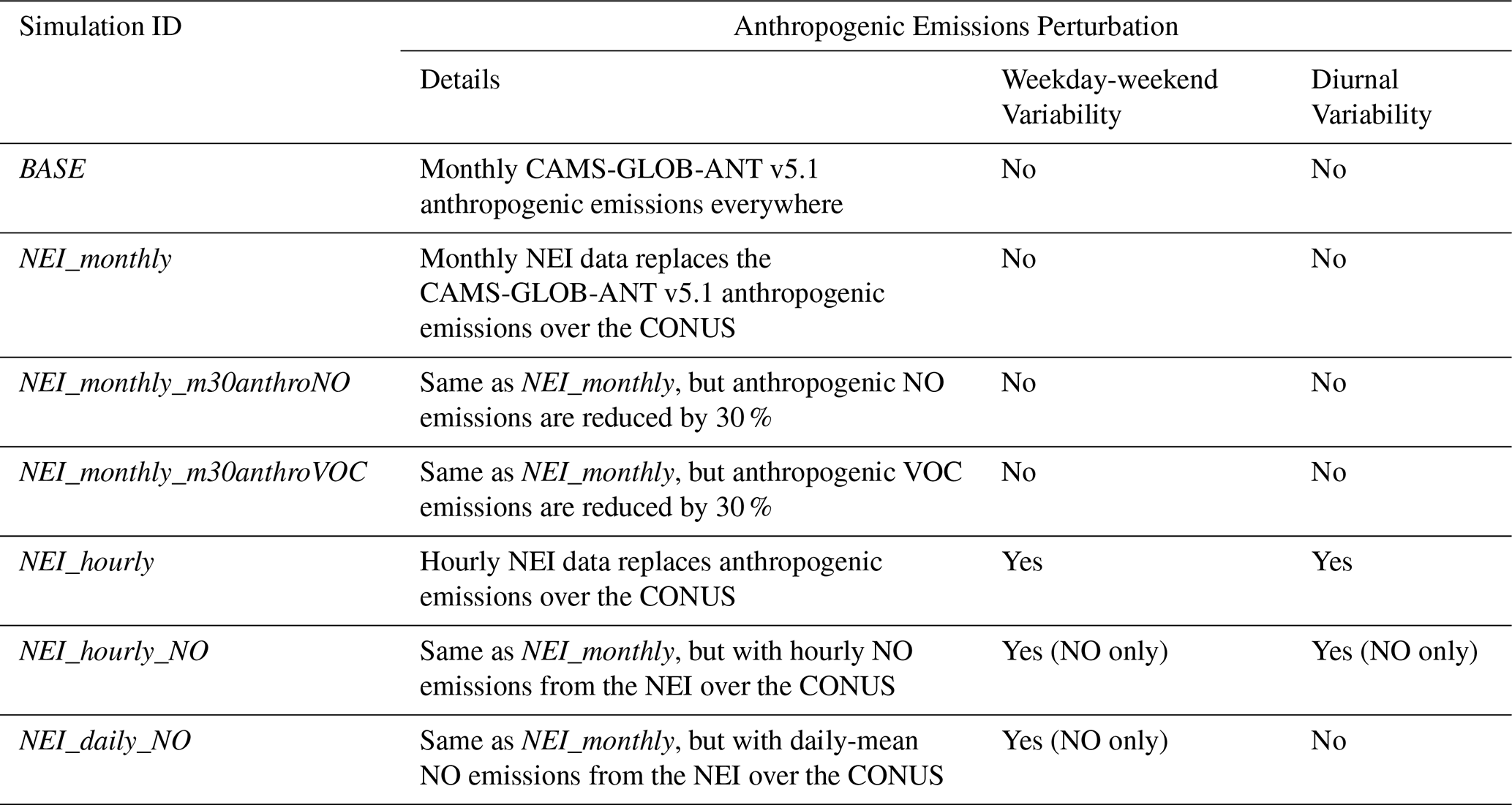
Modifications to the CONUS Anthropogenic Emissions Inventory

The standard global emission inventory in MUSICAv0 is CAMS-GLOB-ANT, which provides monthly averages for 36 emitted compounds within 17 sectors at a spatial resolution of 0.1° × 0.1° (latitude × longitude) (Soulie et al., 2024). Here, we use CAMS-GLOB-ANT version 5.1 (Eskes et al., 2021), which combines the Emissions Database for Global Atmospheric Research (EDGAR) v5 (Crippa et al., 2019) up to 2015 with the Community Emissions Data System (CEDS) (McDuffie et al., 2020) to extend emissions from 2016 to 2021. To evaluate the sensitivity of simulated air pollutant concentrations to the temporal resolution of anthropogenic emissions, we replace the global CAMS-GLOB-ANT baseline inventory with the U.S. Environmental Protection Agency (EPA) National Emissions Inventory (NEI) over the CONUS, which provides more detailed (higher spatial resolution; hourly-varying) regional emissions. We then conduct a series of simulations that differ only in the temporal resolution of NEI emissions (monthly, daily, or hourly) to isolate the model response to the timing of emissions while holding the total emissions for July constant.

The U.S. NEI includes emissions of criteria pollutants, precursors, and hazardous air pollutants (U.S. Environmental Protection Agency, 2024). The NEI is updated every three years and constructed through the Emissions Inventory System (EIS), which collects and integrates data primarily provided by State, Local, and Tribal air agencies. We first process the 2017 NEI (U.S. Environmental Protection Agency, 2022), the most recent pre-COVID inventory available at the time of this study, to generate hourly emissions on a ∼ 0.1° × 0.1° grid over the CONUS (Sect. S3) using sector-specific diurnal profiles to capture within-day as well as day-to-day variations. The 2017 hourly NEI data are then shifted by one calendar day so that the weekday-weekend cycle matches the 2018 calendar and re-gridded (mass-conserving) to the unstructured ne0CONUSne30x8 horizontal resolution using NCAR-developed tools (National Center for Atmospheric Research, 2022a, b). All subsequent references to NEI in this study refer to this adjusted product unless otherwise noted.

Switching from CAMS-GLOB-ANT v5.1 to monthly mean NEI emissions yields widespread decreases in most emitted species across the CONUS, particularly for NO and CO (Fig. S4c). Changes in anthropogenic VOC emissions are also evident (Fig. S4c), but their magnitude remains small compared with biogenic VOC emissions (compare Fig. S5 with Fig. S4a–b; see Sect. S4 for the full list of emitted VOC species). We verified that hourly NEI emissions are read by MUSICAv0 in UTC time with the prescribed diurnal and weekday-weekend variability preserved in local time at the grid-cell level (Sect. S3; Figs. S6 and S7).

To assess the impact of using an alternate anthropogenic emissions inventory and different temporal resolutions of emissions, we conduct four one-month simulations (Table 1): (1) monthly NEI data replace CAMS-GLOB-ANT v5.1 emissions over the CONUS, with CAMS monthly means retained elsewhere (NEI_monthly); (2) as in NEI_monthly but hourly NEI emissions are applied for all species over the CONUS (NEI_hourly); (3) as in NEI_monthly, but only NO is emitted hourly (NEI_hourly_NO); (4) as in NEI_monthly, but NO emissions vary daily and thus include weekday-weekend differences (NEI_daily_NO). Here, anthropogenic NO_x emissions are provided as NO, the predominant emitted form of NO_x. Hourly NEI emissions (NEI_hourly and NEI_hourly_NO) include day-specific diurnal variability (and therefore distinguish between weekdays and weekends), whereas NEI_ daily_ NO removes within-day (diurnal) variability (Table 1). To summarize: the NEI_monthly vs. BASE comparison isolates the effect of changing emission inventories; NEI_hourly vs. NEI_monthly assesses the influence of adding sub-monthly (daily and diurnal) variability for all anthropogenic emissions, NEI_daily_NO vs. NEI_monthly isolates the effect of weekday-weekend differences in NO emissions, and NEI_hourly_NO vs. NEI_ daily_NO isolates the effect of the diurnal changes in NO emission.

We conduct two additional one-month simulations using the NEI_monthly case as the reference to analyze the O₃ production regime under idealized perturbations to anthropogenic NO_x and VOC emissions. In one simulation, we reduce anthropogenic NO emissions by 30 % (NEI_monthly_m30anthroNO) and in another we reduce anthropogenic VOC emissions by 30 % (NEI_monthly_m30anthroVOC) (Table 1). These additional sensitivity simulations provide context for those incorporating the more nuanced changes in the temporal resolution of anthropogenic emissions (Sect. S4).

3 Evaluating the Sensitivity of Simulated Air Pollution to Emission Inventory Choice and Temporal Resolution

To account for regional variation, we divide the CONUS into six regions: West Coast, Mountain, Midwest, Southwest, Northeast, and Southeast (Fig. 1). For each region, Fig. 2 compares modeled (Sect. 2) and observed (Sect. 3.1) July mean surface concentrations of NO₂, O₃, and CO, as well as vertical column densities of tropospheric NO₂ and HCHO and total CO (Sect. 3.2; additional details are in Table S2). We evaluate the model spatial representation of the observations using Spearman's rank correlation coefficient (r_s) and mean bias error (MBE), calculated from monthly mean values at all grid cells within the selected domain. Detailed statistics for July mean values, including the absolute and relative differences in both MBE and root mean square error (RMSE), are provided in Table S2. Our primary focus is on O₃ and its precursors, though for completeness we include evaluations of surface SO₂ and PM_2.5 in Sect. S5 and Table S3. Urban case studies are used to illustrate these effects at the local scale (e.g., a single model grid cell), where responses are most pronounced and easiest to interpret (Fig. 4).

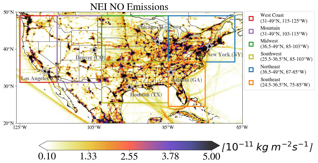
Figure 1 July mean nitric oxide (NO) emissions from the 2017 National Emissions Inventory (NEI) adjusted to 2018, divided into six regions for model analysis: West Coast (red), Mountain (purple), Midwest (green), Southwest (yellow), Northeast (blue), and Southeast (orange). The locations of selected State and Local Monitoring Stations (SLAMS) in six major cities – Los Angeles (CA), Denver (CO), Chicago (IL), Houston (TX), New York City (NY), and Atlanta (GA) – are marked with stars.

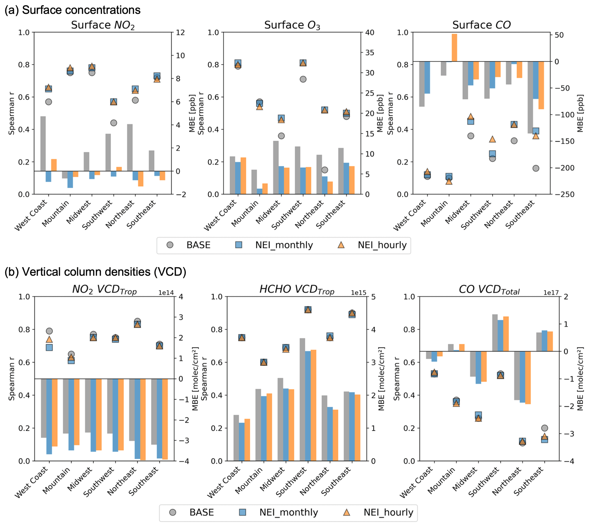
Figure 2 Switching to monthly NEI emissions generally improves spatial correlations and reduces biases compared with observations, whereas changes in the temporal resolution of emissions have smaller effects but regionally these impacts differ. Shown are MUSICAv0-simulated (a) surface concentrations of NO₂, O₃, and CO, and (b) column densities of tropospheric NO₂, tropospheric HCHO, and total CO compared with observations (AQS for surface; TROPOMI for columns) for July 2018 across the six U.S. regions indicated in Fig. 1. Mean bias error (MBE; right axis) is shown as colored bars, and Spearman correlation coefficients (r_s; left axis) are shown as colored markers with distinct shapes. Colors indicate different model simulations (Table 1): BASE (gray bars/circles), NEI_monthly (blue bars/squares), and NEI_ hourly (orange bars/triangles). See Table S2 for detailed statistics, including both the absolute and relative differences in MBE and root mean square error (RMSE).

3.1 Observational Datasets for Model Evaluation

We use measurements collected from State and Local Air Monitoring Stations (SLAMS) that are reported to the U.S. EPA Air Quality System (AQS) for trace gases (O₃, NO₂, CO, and SO₂) and PM_2.5 concentrations (Table S4), downloaded from the AQS AirData portal (https://aqs.epa.gov/aqsweb/airdata/download_files.html, last access: 1 August 2023). To compare MUSICAv0 surface simulations with SLAMS surface measurements, we identify the closest model grid cell based on the latitude and longitude of the SLAMS monitors. We then align hourly concentrations in local time from SLAMS with MUSICAv0 for each species across all CONUS monitors. A limitation of this evaluation is that most SLAMS sites are in urban areas and are influenced by localized effects that cannot be fully resolved by the model at 14 km resolution, which may affect the representativeness of site-level comparisons. The locations of SLAMS used in this study for each species, along with their distribution across CONUS regions and the number of monitors within selected urban grid cells, are shown in Fig. S8.

We select six monitoring stations as examples to examine diurnal patterns at individual sites (Table S5), chosen based on their proximity to major city centers across the CONUS and the availability of continuous NO₂ and O₃ measurements throughout July 2018. Nearby stations with similar diurnal behavior were excluded to avoid redundancy. We do not average across sites as we prefer to preserve distinct local features given differences in monitor availability across cities (Fig. S8).

We also use retrievals from TROPOMI, a nadir-viewing shortwave spectrometer aboard the Sentinel 5 Precursor (S5P) satellite launched in 2017 and operational in 2018. We compare tropospheric vertical column densities (VCD_Trop) of NO₂ (5.5 km × 3.5 km) and HCHO (5.5 km × 3.5 km), along with total vertical column densities (VCD_Total) of CO (5.5 km × 7 km) retrieved from TROPOMI (RPRO Version 02.04.00; last access: 1 December 2023). We select pixels with quality assurance greater than 0.75 (Table S4), which largely excludes cloudy and partly cloudy pixels (van Geffen et al., 2020; Lange et al., 2023). We re-grid the column densities and corresponding averaging kernels (AKs) to a horizontal resolution of 0.15° × 0.15°, slightly coarser than that of the model simulations over the CONUS (approximately 0.125°). TROPOMI uses a priori profiles derived from the TM5-MP global chemistry transport model (Myriokefalitakis et al., 2020), the massively parallel (MP) version of the Tracer Model version 5 (TM5), to simulate the vertical distribution of NO₂, HCHO, and CO, which are provided as supplementary data with the Level-2 products. The TM5-MP model provides data at a 1° × 1° horizontal resolution for the troposphere and upper troposphere-lower stratosphere on 34 hybrid sigma-pressure levels from the surface to approximately 0.1 hPa for retrieving the VCD_Trop of NO₂ and HCHO (Williams et al., 2017). The CO total column density retrievals are based on 50 hybrid sigma-pressure levels from TM5-MP.

To compare modeled column densities with TROPOMI retrievals, we mass conservatively re-grid the hourly MUSICAv0 HCHO, NO₂, CO, and meteorological variables to a 0.15° × 0.15° finite volume grid. We calculate the average between 01:00 and 02:00 p.m. LT (to approximate 01:30 p.m. values) for each region and apply the TROPOMI AKs, linearly interpolated vertically to the MUSICAv0 vertical resolution, to ensure a consistent application of AKs across all MUSICAv0 sensitivity simulations when calculating modeled VCD_Trop of NO₂ and HCHO and VCD_Total of CO. Our interpolation of the TROPOMI AKs to the MUSICAv0 vertical grid generally preserves their vertical structure without introducing unphysical smoothing (Fig. S9). We use the tropopause height diagnosed from the model simulations. Applying AKs to the modeled column enables a more consistent comparison between model simulations and satellite retrievals by accounting for the vertical sensitivity of the satellite instrument. We compare daily 01:30 p.m. VCD_Trop or VCD_Total values across individual grid cells, matching each valid retrieval to the nearest model grid cell. Reported averages include only grid cells with valid retrievals after quality filtering.

3.2 Choice of Monthly Emission Inventory (BASE vs. NEI_monthly) Influences Simulated Air Pollution

We focus on region-specific comparisons with observations across the CONUS (Fig. 2; Tables S2 and S3), as substantial spatial variation suggests that national-level summaries may obscure important regional differences. Across the six CONUS regions, spatial correlations between observed and modeled surface concentrations in the BASE simulation (with the global CAMS-GLOB-ANT emissions) are stronger for NO₂ and O₃ (r_s typically > 0.5) than for CO (r_s= 0.10–0.36) (Fig. 2a; Table S2). Modeled surface concentrations of NO₂ are biased high by 22 %–40 % (2–5 ppb) in all regions except the Mountain region, which shows an average low bias of 18 % (1 ppb). Modeled July mean surface O₃ concentrations are overestimated by 11 %–29 % (6-13 ppb). Surface CO is underestimated by 17 %–87 % (27–140 ppb) compared to SLAMS across all regions. Modeled July mean VCDs (Fig. 2b; Table S2) correlate spatially with TROPOMI NO₂ VCD_Trop (r_s: 0.65–0.85) and HCHO VCD_Trop (r_s=  0.60–0.92), though the correlation is weak for CO VCD_Total (r_s= 0.11–0.53). Modeled NO₂ VCD_Trop is underestimated by 34 %–48 % (∼ 3 × 10¹⁴ molec. cm⁻²), while HCHO VCD_Trop is overestimated by 15 %–24 % (1–4 × 10¹⁵ molec. cm⁻²) across the six regions. CO VCD_Total is underestimated by 2 %–11 % (3–18 × 10¹⁶ molec. cm⁻²) in the West Coast, Midwest, and Northeast, but overestimated by 2 %–8 % (3–14 × 10¹⁶ molec. cm⁻²) in the Mountain, Southwest, and Southeast regions.

Compared to the BASE case, NEI_monthly (Table 1) improves spatial correlations (r_s) and reduces model biases (MBE and RMSE) for surface NO₂, CO, and O₃ concentrations, particularly in the Northeast (Fig. 2a; Table S2). Differences in simulated surface NO₂ and CO between NEI_monthly and BASE (Fig. 3a) reflect emissions changes in NO and CO due to the shift from CAMS-GLOB-ANT v5.1 to NEI (Fig. S4). Lower NEI NO emissions (Fig. S4c) reduce regional mean NO₂ concentrations by 1–6 ppb, bringing high biases down to within 1 ppb but exacerbating the low bias in the Mountain region to −2 ppb (Fig. 2a). CO concentrations increase relative to the BASE simulation (Fig. 3a), improving the surface CO underestimation by 13 %–55 % (20–65 ppb), although low biases of 1 %–33 % (2–71 ppb) remain (Fig. 2a). For secondary pollutants like O₃, changes in concentrations do not directly mirror emissions perturbations. Surface O₃ concentrations decrease in NEI_monthly relative to BASE, reducing modeled surface O₃ biases relative to SLAMS by 2 %–11 % (approximately 1–6 ppb) on average across the six regions (Figs. 2a and 3a). However, model biases of 3 %–21 % (1–8 ppb) remain across all regions, particularly on the West Coast (NEI_monthly in Fig. 2a).

There are minimal to no changes in r_s for HCHO VCD_Trop, while NO₂ VCD_Trop shows weaker correlations and worsening model biases (Fig. 2b; Table S2). Changes in CO VCD_Total exhibit large regional variability (Fig. 3b). Switching to NEI consistently decreases both surface and column NO₂ but not CO (Fig. 3). Compared to BASE, NEI_monthly worsens the model underestimates of NO₂ VCD_Trop by 16 %–21 % (∼ 1 × 10¹⁴ molec. cm⁻²) but decreases overestimates of regional mean HCHO VCD_Trop by approximately 2 % (0.2–4 × 10¹⁴ molec. cm⁻²) across all regions (Fig. 2b). CO VCD_Total changes little (Fig. 3b), with the sign of the model bias unchanged from BASE (Fig. 2b).

Biases in trace gas columns do not always match those at the surface. For instance, surface NO₂ is biased high in some regions especially in BASE, while NO₂ VCD_Trop are consistently biased low relative to TROPOMI (Fig. 2). These different biases in the surface versus column can arise from several factors that are independent of surface emission magnitude, including: (i) vertical sensitivity and representativeness, given that satellite columns reflect vertically weighted pixel means whereas surface observations are point measurements; and (ii) retrieval uncertainties, including assumptions in the air mass factor calculation and the stratosphere-troposphere separation applied to derive tropospheric NO₂ columns (van Geffen et al., 2020). In addition, prior global chemistry models have been shown to underestimate background NO₂ VCD_Trop relative to satellite products, partly due to uncertainties in free-tropospheric NO_x chemistry (e.g., $\mathrm{NO}/{\mathrm{NO}}_{\mathrm{2}}$ ratios and partitioning among reactive nitrogen species) (van Geffen et al., 2022; Shah et al., 2023; Silvern et al., 2018, 2019).

3.3 Incorporating Hourly Variations in Emissions (NEI_hourly) Affects Monthly Mean Pollutant Concentrations

The surface NO₂ and O₃ concentration changes between NEI_hourly and NEI_monthly are, in some regions, similar in magnitude to those between NEI_monthly_m30anthroNO (a 30 % reduction in anthropogenic NO emissions) and NEI_monthly, but the spatial patterns differ markedly (Fig. 3a), reflecting the temporal redistribution of emissions. Although the overall agreement with observations changes only slightly (r_s, MBE, and RMSE; Fig. 2 and Tables S2 and S3), the direction and magnitude of concentration changes vary across regions, especially between urban and rural areas and between the western and eastern CONUS (Figs. 3 and 4).

The largest July regional-mean difference in surface NO₂ concentrations (NEI_hourly − NEI_monthly) occurs on the West Coast (+16%, or +0.3 ppb), while NO₂ decreases most in the Northeast (−7 %, −0.1 ppb) (Fig. 3a). As a result, the model shifts from underestimation to overestimation on the West Coast, while the underestimation in the Northeast is exacerbated versus the surface NO₂ SLAMS observations (Fig. 2a). Changes in surface CO are small and spatially varied, with regional mean increases of 2 %–7 % (4–10 ppb) in the West Coast, Mountain, Midwest, and Southwest, and decreases of about 3 % (∼ 5 ppb) in the Northeast and Southeast (Fig. 3a). Changes in NO₂ VCD_Trop and CO VCD_Total largely mirror the surface patterns (Fig. 3b).

High model biases persist for surface O₃ concentrations (5 %–20 %; 3–9 ppb) after incorporating hourly variations in emissions (NEI_hourly in Fig. 2a). Monthly mean surface O₃ concentrations decrease by up to ∼ 2 % (< 1 ppb) in the Midwest, Northeast, and Southeast, while increases of up to ∼ 3 % (1–4 ppb) in other regions slightly worsen model overestimation. Previous studies also find model overestimates of near-surface O₃, with the most significant biases in the Southeast U.S., possibly reflecting uncertainties in isoprene–NO_x–O₃ chemistry, inaccuracies in dry deposition and forest canopy parameterization, and overestimates in NO_x emissions (Baublitz et al., 2020; Fiore et al., 2009; Makar et al., 2017; Martin et al., 2014; Schwantes et al., 2020; Travis et al., 2016). Although surface HCHO observations are unavailable for evaluation, modeled changes remain under 3 % and follow similar spatial patterns to those of surface O₃ (Fig. 3a). Monthly mean HCHO VCD_Trop decreases in the Midwest, Northeast, and Southeast but increases in other regions, mirroring the regional pattern of surface HCHO changes (Fig. 3), though a general high model bias of 14 %–23 % (1–3 × 10¹⁵ molec. cm⁻²) persists (Fig. 2b; Table S2).

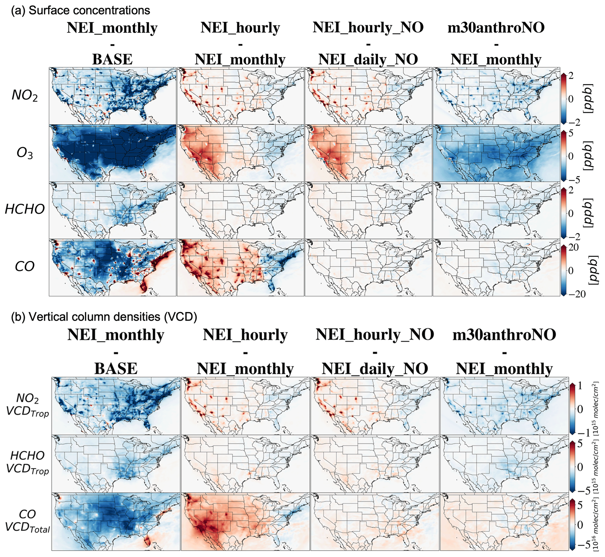
Figure 3 Changes produced by switching from BASE to NEI_monthly (left column), and by resolving hourly variations in NO emissions produces distinct spatial responses in July monthly mean (middle two columns; see Table 1): (a) surface concentrations, with absolute changes comparable to those from a uniform 30 % reduction in monthly mean NO emissions (right column); and (b) column densities, which generally mirror surface responses. Consistent color-bar ranges are used for each variable. See Fig. S2b for differences in surface SO₂ and PM_2.5.

3.4 Model Evaluation: Diurnal Variability and Weekday-Weekend Differences

Our model simulations (Table 1) broadly capture day-to-day variations in surface NO₂ and O₃ at the six urban sites (Fig. S10), but they tend to overestimate both the daily range and the weekday-weekend differences and misrepresent the timing of peak concentrations in most cities (Fig. S11). The exaggerated daily range reflects opposite model biases at different times of day: the model overestimates nighttime NO₂ (when concentrations are highest) and fails to capture the nighttime minimum in O₃, while at midday it underestimates NO₂ and overestimates O₃ (Fig. S11). As expected, simulations with day-to-day variations in emissions better capture weekday-weekend concentration differences compared to NEI_monthly, though the diurnal shape still does not fully capture observations (see the right column of Fig. S11). The model also misrepresents the timing of daily peaks. For example, the simulated NO₂ maximum occurs at 06:00 a.m. in Los Angeles, about two hours earlier than observed (Fig. S11).

It is challenging for models to accurately represent the complex diurnal processes that shape near-surface concentrations, including boundary-layer evolution (Adams et al., 2023). Our MUSICAv0 simulations use the standard CAM6 planetary boundary layer parameterization, the Cloud Layers Unified By Binormals (CLUBB) (Bogenschutz et al., 2018; Danabasoglu et al., 2020). While prior evaluation within the CESM2/CAM6 framework shows that the scheme generally captures the broad diurnal and seasonal structure of boundary-layer behavior, overly strong nocturnal mixing leads to errors in the timing of the morning transition although the specific biases vary across regions and seasons (Holtslag et al., 2013; Schwantes et al., 2022; Stjern et al., 2023). These biases will be reflected in the simulated diurnal amplitude and timing of near-surface concentration peaks and their relationship to the underlying temporal profile of emissions. Errors may also arise from the NEI diurnal profiles applied in this study, which are sector-specific and derived from activity-based temporal allocation methods whose accuracy at local scales is uncertain. In addition, comparisons between model grid-cell means and individual SLAMS sites inevitably involve representativeness differences that may contribute to mismatches.

4 Sensitivity to Resolving Hourly Variations in Nitric Oxide Emissions

Imposing hourly-varying emissions results in spatially heterogeneous changes even in the monthly mean surface NO₂, O₃, and HCHO concentrations, with strong west-east and urban-rural contrasts (Figs. 3–5). We demonstrate that these simulated responses produced by switching from NEI-monthly to NEI_hourly are primarily driven by the hourly variations in NO emissions, evidenced by minimal changes between NEI_hourly_NO and NEI_hourly (< 0.5 % for NO₂, HCHO, and O₃). Comparisons between NEI_daily_NO and NEI_monthly, and between NEI_ hourly_NO and NEI_daily_NO, indicate that these spatial patterns are shaped by switching from daily mean to hourly varying NO emissions (Figs. 3 and S12). As illustrated in Fig. 6, switching from daily mean to hourly NO emissions increases daytime and decreases nighttime emissions, with larger differences on weekdays, thereby influencing surface NO_x concentrations and secondary pollutants like O₃.

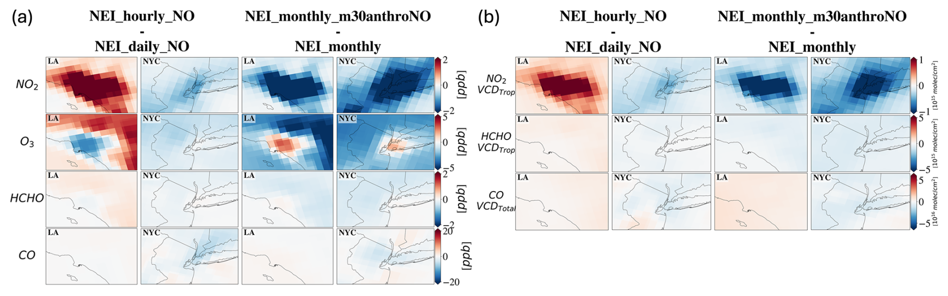
Figure 4 Changes produced over Los Angeles (LA) and New York City (NYC) by resolving hourly NO emissions (first two columns) versus a uniform 30 % decrease in anthropogenic NO emissions (two right-most columns) for (a) surface concentrations and (b) column densities.

4.1 West-East Contrasts in Surface Pollutant Responses

To understand the broader impacts of incorporating hourly NO emissions, we begin by examining regional contrasts in July daytime (09:00 a.m.–05:00 p.m. local time) responses across the CONUS, as shown in Fig. 5. Panel a maps the differences in surface NO, NO₂, O₃, and HCHO concentrations (NEI_hourly_NO minus NEI_ daily_NO), while panel b summarizes the meridional means in 5° longitudinal bins. These plots highlight a west-to-east gradient in pollutant responses driven solely by adding the diel cycle to NO emissions. To help interpret this spatial variability, panel c presents the corresponding NEI_daily_NO daytime emissions and key meteorological variables, including surface temperature, planetary boundary layer height (PBLH; m a.g.l.), relative humidity, and NO₂ lifetime against dry deposition.

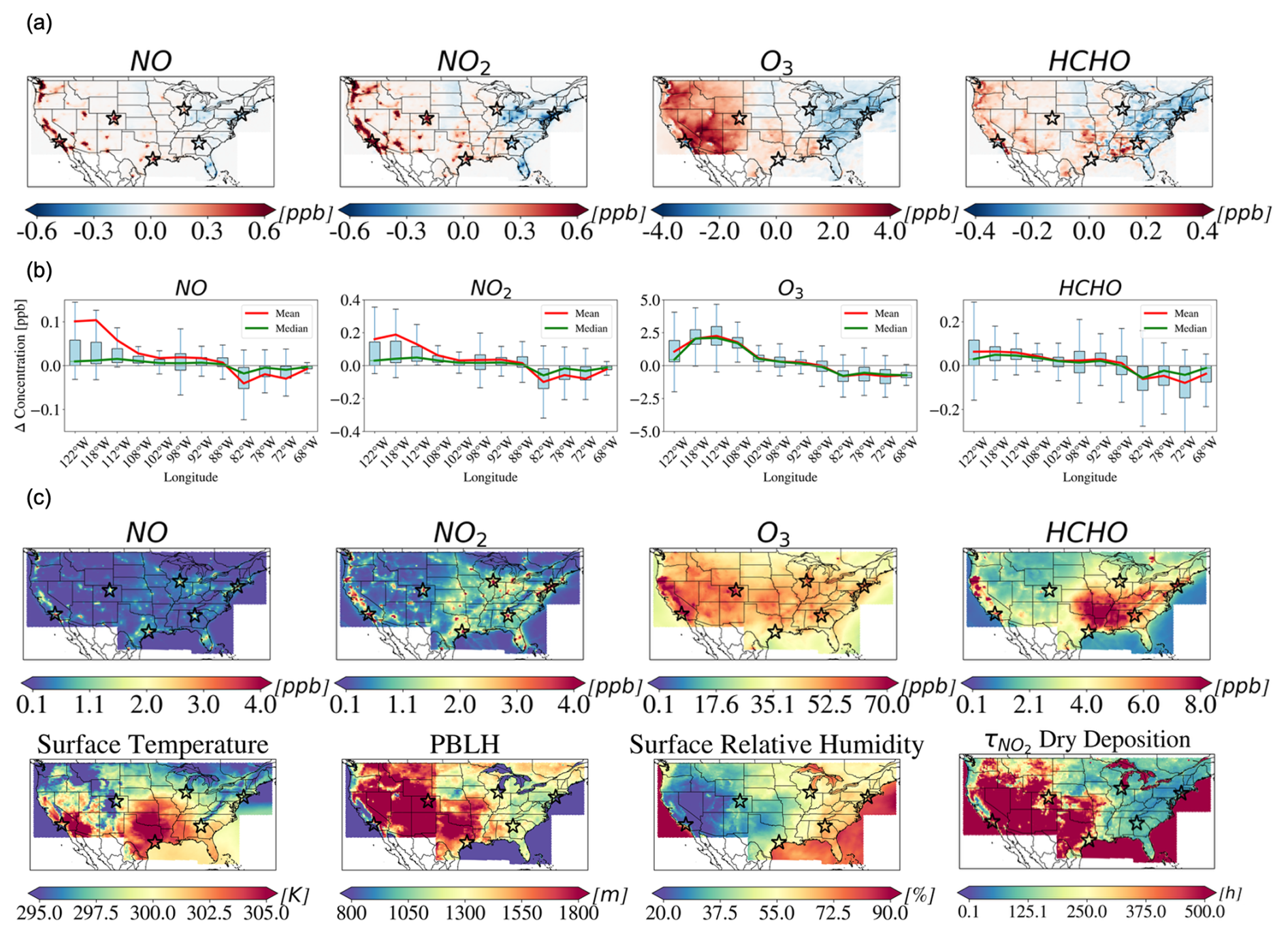
Figure 5 Resolving hourly NO emissions results in contrasting surface responses between the western and eastern CONUS and between urban and rural areas. Panel (a) shows monthly mean July daytime (09:00 a.m.–05:00 p.m. local time) differences in simulated surface concentrations of NO, NO₂, O₃, and HCHO (NEI_hourly_NO minus NEI_ daily_ NO). Panel (b) provides a meridional summary of the July daytime differences shown in panel (a), with values averaged within 5° longitude bins across CONUS latitudes (23–50° N). Each boxplot shows the interquartile range (25th–75th percentiles) within each longitude bin, with whiskers extending to 1.5 × interquartile range (outliers excluded); red and green lines denote the mean and median, respectively. The horizontal line marks zero change. Panel (c) displays monthly mean July daytime values from the NEI_ daily_NO simulation. The first row presents surface concentrations of NO, NO₂, O₃, and HCHO, and the second row includes relevant meteorological variables: surface temperature, planetary boundary layer height (PBLH; m a.g.l.), and surface relative humidity. The rightmost plot in the second row shows the surface NO₂ lifetime against dry deposition loss.

Polluted urban regions with higher NO emissions (Fig. 1) show more pronounced NO_x concentration responses (Figs. 3 and 4). In the western CONUS, July daytime (09:00 a.m.–05:00 p.m.) monthly mean surface NO and NO₂ concentrations increase by up to 8 and 6 ppb, respectively, in urban areas in NEI_hourly_NO simulation relative to NEI_daily_NO (Fig. 5a–b). In contrast, monthly mean daytime surface NO and NO₂ decrease over the eastern CONUS by up to ∼ 1 ppb, respectively, with the largest changes also concentrated in urban areas. However, changes in surface O₃ do not always coincide with the largest NO_x concentration changes. In the eastern CONUS, O₃ decreases by up to ∼ 2 ppb (Fig. 5a–b), with the largest reductions over the polluted urban centers, consistent with prior findings (e.g., Jo et al., 2023). In contrast, monthly mean O₃ increases of up to 8 ppb occur over the western CONUS along the edges of urban areas (Fig. 5a). This spatial pattern points to enhanced NO_x sensitivity at the periphery of NO_x-saturated western urban cores; similar patterns occur in the NEI_ monthly_ m30anthroNO sensitivity simulation relative to the BASE case, where the 30 % reduction in anthropogenic NO emissions yields the largest O₃ changes in surrounding rural areas (Figs. 3 and 4). In the West, the mean of the NEI_hourly_NO minus NEI_ daily_ NO differences exceeds the median (Fig. 5b), driven by large NO_x increases in a few urban grid cells. In the East, the larger mean decreases relative to the median similarly reflect strong but localized NO_x decreases. By contrast, O₃ differences show closer agreement between mean and median across both regions, suggesting more spatially uniform impacts (Fig. 5c).

These spatial patterns are shaped by a complex interplay of background anthropogenic and biogenic emissions, local photochemical conditions, meteorology (especially boundary layer dynamics and transport), and deposition. In July, the East Coast has higher background NO emissions, approximately 70 % higher over the Northeast region than over the West Coast (Fig. 1). In the western U.S., anthropogenic emissions tend to occur in more localized hotspots in contrast to the continuous, corridor-like pattern in the eastern U.S., consistent with population density and urban clustering (Fig. S4a). Biogenic emissions, dominated by isoprene and monoterpenes, are highest and widespread across the eastern and southern CONUS (Fig. S5). Switching to hourly emissions generally increases daytime NO (Fig. 6), yet the resulting impact on surface concentrations across the CONUS (Fig. 5a) differs notably from the response to a uniform 30 % reduction in anthropogenic NO emissions (Fig. 3). This finding indicates that the timing of anthropogenic emissions perturbations with respect to other processes like meteorology (Fig. 5c), biogenic emissions, and deposition shape the contrasting changes between the western and eastern CONUS. For example, shallower daytime PBLH such as over the eastern CONUS can limit vertical mixing while enhancing both photochemical reactions and surface deposition (Wu et al., 2024). Together with higher humidity, these processes may contribute to a shorter NO₂ lifetime in the eastern CONUS during July 2018. We explored the possibility of a persistent synoptic-scale east-west dipole in air stagnation, defined according to the meteorological criteria of Wang and Angell (1999), but did not find any evidence for such a feature.

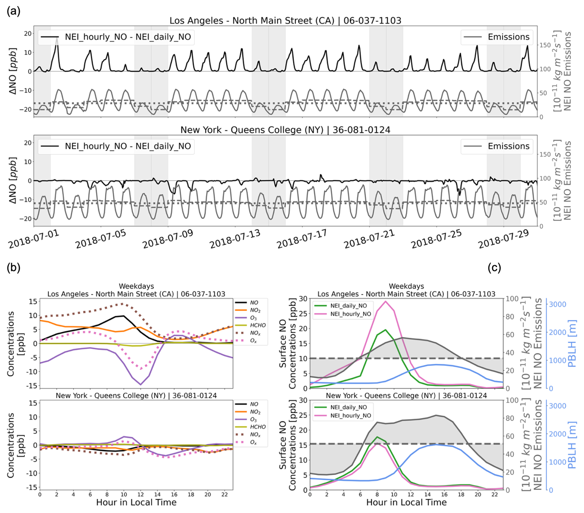
Figure 6 Despite similar diurnal variation in NO emissions – higher during daytime, lower at night – Los Angeles and New York City show different pollutant responses reflecting city-specific emission timing, boundary layer dynamics, and local photochemistry. (a) Hourly time series of July differences in surface NO concentrations between NEI_ hourly_NO and NEI_daily_NO (black solid lines), alongside hourly (solid gray), daily mean (dashed), and monthly mean (dotted) NO emissions. Weekend days are shaded in gray. The lower-than-typical weekday emissions on 3 July 2018 reflect the July 4th holiday pattern in the 2017 NEI data following the shift to the 2018 calendar. Also shown are July 2018 weekday average (b) hourly surface concentration differences between NEI_ hourly_NO and NEI_daily_NO for NO (black), NO₂ (orange) O₃ (purple), and HCHO (olive green), with NO_x (≡ NO + NO₂; brown) and O_x (≡ O₃+ NO₂; pink) shown as dotted lines; (c) hourly NO concentrations from NEI_ daily_NO (green) and NEI_hourly_NO (pink), NO emissions (gray) and PBLH (blue) for Los Angeles (top) and New York City (bottom). Solid lines represent the mean weekday diel cycle of emissions, while dashed lines show the corresponding weekday mean across all hours. Weekend days show similar patterns but with smaller magnitudes of change (Fig. S13). Results for all sites (including Chicago, Denver, Houston, and Atlanta; see Fig. 1), with both weekday and weekend averages shown for panels (b)–(c), are provided in Fig. S13.

4.2 Urban Case Studies: Los Angeles vs. New York City

To further investigate the regional contrasts introduced in Sect. 4.1, we examine two representative urban centers, Los Angeles (CA) and New York City (NY), to show how local-scale meteorology and photochemistry interact with hourly NO emission patterns to produce opposite-signed responses in NO_x and O₃ concentrations. Figure 6 compares NEI_ hourly_NO and NEI_daily_NO simulations, showing (a) time series of NO emissions and surface NO concentration differences, (b) July weekday-averaged diel differences in NO, NO₂, O₃, and HCHO, and (c) weekday-averaged diel cycles of NO emissions, surface NO, and PBLH. Weekend patterns are similar but generally smaller in magnitude (see Fig. S13). Figure 7 presents July daytime O₃ production rates (P(O₃), diagnosed in MUSICAv0 as chemical O₃ production from reactions of NO with the hydroperoxy radical and organic peroxy radicals) binned by surface NO_x concentrations for the NEI_monthly, NEI_hourly_NO, and NEI_ monthly_ m30anthroNO simulations. Box plots summarize the distribution of P(O₃) within uneven NO_x concentration bins (e.g., 0–1, 1–2, …, 5–10, 10–15, …, > 50 ppb); color-coded points highlight values during morning, noon, and afternoon periods. Figures S7, S13 and S14 include our findings for all major cities shown in Fig. 1.

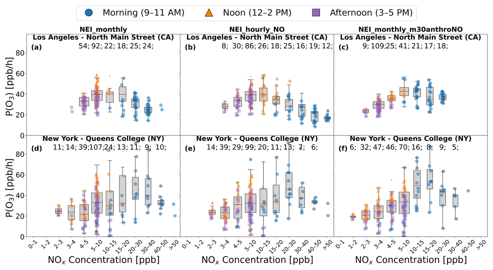
Figure 7 Modeled hourly P(O₃) (ppb h⁻¹) versus surface NO_x concentrations (ppb) for July daytime hours (09:00 a.m.–05:00 p.m.) in NEI_monthly (left column), NEI_ hourly_NO (middle), and NEI_monthly_m30anthroNO (right) sampled at the selected Los Angeles (CA; a–c) and New York (NY; d–f) monitoring site. Colored points highlight local morning (09:00–11:00 a.m., blue circles), noon (12:00–02:00 p.m., orange triangles), and afternoon (03:00–05:00 p.m., purple squares). Boxplots summarize the distribution of P(O₃) within uneven NO_x bins (e.g., 0–1, 1–2, …, 5–10, 10–15, …, > 50 ppb) plotted at equal spacing along the x axis. Only bins containing at least five data points are shown, and the sample size is indicated above each corresponding box; box widths are scaled to the sample size. Results for additional sites (Chicago, Denver, Houston, and Atlanta) are included in Fig. S14.

Comparing NEI_hourly_NO to NEI_ daily_NO, surface NO_x concentrations decrease in New York City but increase in Los Angeles, especially during the morning rush hour when the boundary layer is growing (Fig. 6b–c). Monthly mean surface O₃, however, decreases in both Los Angeles and New York City, though the magnitudes differ (Fig. 4a). Surface O₃ decreases most in Los Angeles on weekdays between 09:00 a.m. and 03:00 p.m., outweighing a smaller late-afternoon increase (03:00–06:00 p.m.) (Fig. 6b). In New York City, the net monthly mean decrease is minimal because modest reductions from noon to evening (12:00–06:00 p.m.) only slightly exceed the morning increase (08:00 a.m.–12:00 p.m.) (Fig. 6b).

To assess the sensitivity of P(O₃) to NO_x and VOC, we compare P(O₃) in NEI_monthly_m30anthroNO and NEI_monthly_m30anthroVOC with NEI_monthly (Table 1). All three simulations indicate that New York City and Los Angeles are generally NO_x-saturated, with surface O₃ increasing as NO emissions decrease (Fig. 4a) and little change in response to the 30 % reduction in anthropogenic VOC emissions (< 0.5 % across all regions; not shown). Previous studies have shown that O₃ production tends to become more NO_x-sensitive around noon and in the afternoon, when photochemical conditions are most favorable for O₃ formation (Tao et al., 2022). In contrast, the model indicates a P(O₃) peak during the late morning in both New York City and Los Angeles, particularly in NEI_monthly_m30anthroNO (Fig. 7c, f). Compared to NEI_monthly (Fig. 7a, d), NEI_monthly_m30anthroNO (Fig. 7c, f) shifts the NO_x concentration bins associated with high P(O₃) toward lower NO_x in both Los Angeles and New York City. For example, in Los Angeles, the highest-NO_x conditions (> 30 ppb) shift into lower NO_x bins (< 30 ppb) (Fig. 7a, c).

Incorporating hourly NO emissions (NEI_ hourly_NO) reduces July mean daytime P(O₃) relative to NEI_monthly by ∼ 2 ppb h⁻¹ in Los Angeles and ∼ 0.3 ppb h⁻¹ in New York City. Using hourly NO emissions (NEI_hourly_NO) increases the density of values in the highest NO_x bins in Los Angeles while maintaining similar P(O₃) values in those bins (Fig. 7b), extending the high-NO_x tail of the P(O₃)-NO_x distribution into more strongly NO_x-saturated conditions (compare Fig. 7a vs. Fig. 7b). This enhanced high-NO_x tail reflects larger morning NO_x concentrations, when the chemical regime is most NO_x-saturated and O₃ production is suppressed. Although conditions become more NO_x-sensitive later in the afternoon (Fig. 7b), the larger O₃ decrease during late morning to early afternoon (∼ 09:00–14:00 LT; Fig. 6b) dominates the net monthly mean O₃ concentration response in Los Angeles (Fig. 4a). The more temporally concentrated (peaky) emission profile and shallower daytime PBL heights in Los Angeles compared to New York City (Fig. 6c) likely amplifies NO_x accumulation, reinforcing a NO_x-saturated regime. We find that Los Angeles, Denver, and Houston show broadly similar responses to hourly versus monthly mean NO emissions, while New York City, Chicago, and Atlanta exhibit distinct behavior (Figs. S13 and S14).

4.3 Implications for Satellite-Based NO_x Emission Constraints

Our results in Sect. 4.1 and 4.2 show that resolving hourly NO emissions changes simulated NO₂ VCD_Trop even when the total monthly emissions are the same. Given that NO₂ VCD_Trop observations from satellites are commonly used to derive top-down constraints on NO_x emissions, differences in the timing of emissions in models used for such inversions may alter the inferred emission estimates. NO_x emissions are sometimes inferred using proportional scaling or mass-balance approaches, in which a priori emissions are adjusted based on the ratio of observed to modeled NO₂ columns, for example with chemical transport models that implicitly represent the impacts of transport and chemistry along with emissions on atmospheric concentrations (Lamsal et al., 2011, 2014; Martin et al., 2003). More formal inverse modeling and data assimilation frameworks exist but similarly depend on satellite overpass-time NO₂ columns and model representations of diurnal variability (Goldberg et al., 2019; Miyazaki and Eskes, 2013).

To estimate potential biases in the inferred NO emission magnitude arising from model representation of diurnal emission timing, we perform a simple, one-month scaling-based approach for July 2018 (details in Sect. S6). In this section, Ω denotes NO₂ VCD_Trop and E anthropogenic NO emissions. While our illustrative simple framework assumes a local relationship between Ω and E, we emphasize that Ω will generally reflect emissions from multiple model grid cells given the NO_x lifetime and transport timescales. Transport, chemistry, and lifetime effects are implicitly accounted for through the forward model but are not explicitly inverted. Accordingly, $(\mathrm{\Delta }E/E{)}_{\mathrm{est}}$ in Fig. 8 should be interpreted as an estimate of the potential bias in inferred emission magnitude rather than as a quantitative emission inversion. By comparing NEI_hourly_NO and NEI_monthly to isolate the effect of NO emission timing alone since both simulations use identical monthly-integrated emissions, we find that the inferred timing-representation bias is small on average over the CONUS (+1.8 %) but spatially variable, with regional mean values of 1 %–8 % in the western U.S. and approximately −3 % to −2 % in the Northeast and Southeast (Fig. 8; Table S6). City-scale values are larger, reaching +26 % in Los Angeles, +30 % in Denver and −7 % in New York City (Table S6).

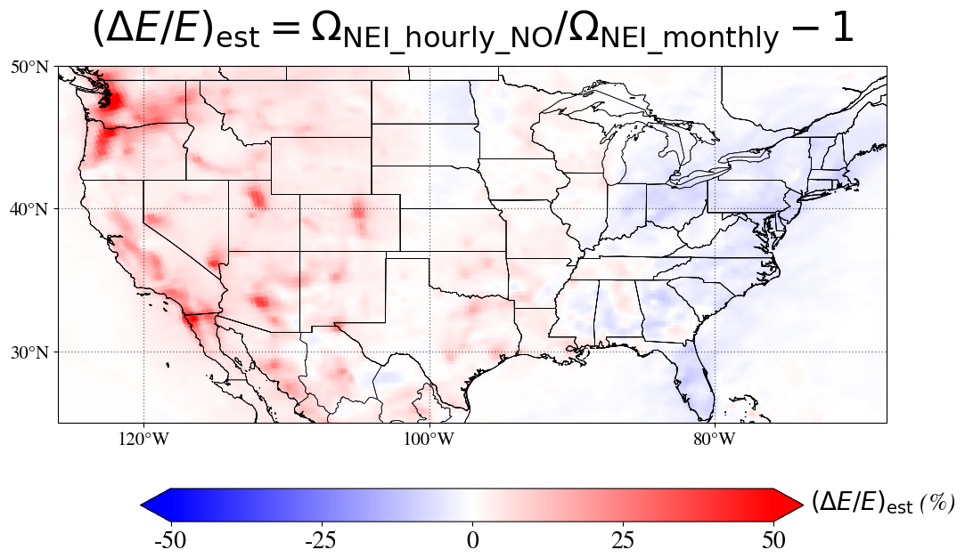
Figure 8 Estimated potential relative biases ($(\mathrm{\Delta }E/E{)}_{\mathrm{est}}$; %) in July 2018 anthropogenic NO emissions magnitude (E) resulting from neglecting hourly NO emissions, derived by comparing July-mean tropospheric NO₂ columns (Ω) simulated in NEI_ hourly_NO versus NEI_monthly. Regional and city-scale statistics are provided in Table S6; see Sect. S6 for detailed methods.

5 Discussion and Conclusions

We demonstrated that inclusion of hourly variations in NO emissions in the MUSICAv0 model produces substantial changes in NO_x and O₃ concentrations, even in monthly averages, comparable in magnitude to those associated with an idealized 30 % reduction in NO emissions (Figs. 3 and 4). In contrast to a uniform 30 % reduction in NO_x, however, the changes in response to the timing of NO emissions differ between urban and rural areas and between the eastern and western U.S., reflecting region-specific emission patterns, photochemistry, and meteorological conditions (Fig. 5). Monthly mean daytime surface O₃ concentrations over the CONUS in July differ by up to 7 ppb (11 % for NEI_hourly relative to NEI_monthly; Fig. 5), large enough to affect model-based conclusions regarding regional attainment of the U.S. NAAQS for O₃. We also find differences in O₃ production regimes across cities: for example, a shift toward more NO_x-saturated conditions in Los Angeles but toward stronger NO_x sensitivity in New York City when hourly variations in NO emissions are included (Figs. 6 and 7).

When we impose hourly variations in NO emissions, monthly mean surface NO₂ increases over the western CONUS by up to ∼ 6 ppb during the daytime. In contrast, the eastern CONUS with its higher NO and biogenic VOC emissions, larger dry deposition flux rates, more humid conditions, and shallower PBLH – all of which favor a shorter NO₂ lifetime – experiences daytime NO₂ decreases of up to ∼ 1 ppb (Fig. 5). Spatial changes in simulated VCD closely follow those in surface concentrations (Figs. 3 and 4). Using a simple scaling-based analysis, we show that resolving hourly emissions, even with identical monthly total NO emissions, has the potential to alter NO emission magnitudes inferred from monthly-averaged satellite-retrieved NO₂ VCD_Trop combined with model column-to-surface relationships. For July 2018, we show that neglecting hourly variability in anthropogenic NO emissions leads to spatially heterogeneous biases in the estimated emissions that are generally modest at the regional scale (a few percent) but substantially larger at the grid-cell level, with absolute relative differences ranging from ∼ 1 % to > 50 % and locally reaching approximately −12 % to +56 % (Fig. 8).

Since August of 2023, the TEMPO instrument aboard a geostationary satellite is now providing continuous daytime measurements of trace gases over North America (Naeger et al., 2021; Zoogman et al., 2017). Similar geostationary retrievals have been available over East Asia since 2020 from the Geostationary Environment Monitoring Spectrometer (GEMS), with recent studies demonstrating its capability to capture diurnal variations in NO₂ VCD_Trop (Edwards et al., 2024; Park et al., 2025; Yang et al., 2024). Our results show that neglecting hourly variations in emissions introduces biases when interpreting monthly mean concentrations from once-daily polar-orbiting satellite overpasses, potentially aliasing sub-daily emission variability into top-down NO_x emission estimates. Emerging geostationary observations now make it possible to evaluate these intra-day effects directly to refine constraints on emission timing as well as related photochemical processes.

Although our analysis focuses on July 2018, the differences we identify due to the temporal resolution of emissions are broadly relevant, though their local magnitude will vary across years with both emissions and meteorology. Recent trends since 2018 could modulate the magnitude of these effects, including: the continued decline in anthropogenic NO_x emissions (Christiansen et al., 2024); increases in temperature-sensitive soil NO_x and biogenic VOCs (Geddes et al., 2022); more frequent heat waves and stagnation events (Gao et al., 2023); and episodic wildfires (Abatzoglou et al., 2025). Lower NO_x emissions and flatter diurnal shapes would likely reduce the differences between using hourly and daily or monthly mean emissions, whereas more stagnant conditions could amplify the O₃ sensitivity to the timing of precursor emissions through enhanced localized photochemistry and deposition. While we analyzed diurnal emission cycles within the CONUS during summer, similar sensitivities are likely to occur in source regions elsewhere, underscoring the need to better characterize diurnal emission cycles and the corresponding chemical responses of air pollutants in other seasons and world regions.