Variability of ice supersaturated regions at flight altitudes: evaluation of ERA5 reanalysis using IAGOS in situ measurements

Contrail cirrus is a major contributor to aviation's radiative forcing. Avoiding persistent contrail formation has been suggested as a measure to reduce the climate impact of aviation, requiring accurate forecasts of ice supersaturated conditions, where the relative humidity over ice (RHi) exceeds 100 %. Numerical weather prediction models and reanalysis products often underestimate or do not account for ice supersaturation. This study evaluates ice supersaturated regions (ISSRs) in the ECMWF ERA5 reanalysis dataset using In-service Aircraft for a Global Observing System (IAGOS) measurements over tropical and extratropical regions in the upper troposphere and lower stratosphere from 2011 to 2022. It considers seasonal and vertical differences, and how cloudy and clear-sky conditions affect ERA5’s ability to predict ISSRs. ERA5 underestimates ISSR occurrence due to a dry bias in RHi; the equitable threat score (ETS) is 0.2–0.4, indicating a weak to mediocre skill. Lowering the ERA5 RHi threshold improves ISSR prediction, with the largest improvements for RHi between 85 % and 95 %, although the optimal threshold varies with distance to the tropopause, region and season. Clear-sky conditions result in an ETS of 0.05–0.18, while the ETS is mostly below 0.1 in cloudy conditions, indicating an almost random relationship. In clear-sky conditions, lowering the threshold to 85 % increases the ETS by approximately 0.1. In cloudy conditions, lowering the threshold shows little benefit because increases in correctly predicted ISSRs are offset by increases in false positives. These findings improve our understanding of ISSR variability and has implications for accurate assessment of persistent contrail formation.

1 Introduction

The aviation industry is a significant contributor to anthropogenic climate change. In 2018, aviation accounted for 2.5 % of the world's CO₂ emissions (Lee et al., 2021). Aviation has also been estimated to contribute to 3.5 % to 5 % of global anthropogenic radiative forcing (Lee et al., 2021). The anthropogenic radiative forcing is due to CO₂ and non-CO₂ emissions, which include NO_x emissions, H₂O, soot, contrails, and contrail cirrus (Lee et al., 2009). The best estimate of contrail cirrus effective radiative forcing is almost twice as large as that of CO₂, but is also subject to a much larger uncertainty range than that of CO₂ (Lee et al., 2021). This is due to a number of uncertainty sources in the evaluation of contrail cirrus, related to the radiative transfer calculations, the upper tropospheric water budget and the modelling of contrail cirrus (Lee et al., 2021).

One solution to lowering the climate impact of aviation is to minimise the radiative forcing due to contrail cirrus. Contrail cirrus is the result of the dispersion of persistent contrails. Contrails form when the Schmidt-Appleman criterion (SAC) is met (Schumann, 1996), and persist when the ambient air is supersaturated with respect to ice, i.e. relative humidity over ice (RHi) is greater than 100 % (Gierens et al., 2020a; Wolf et al., 2025). A region where the latter occurs is called an ice supersaturated region (ISSR) (Reutter et al., 2020). Reducing persistent contrails can be realised by avoiding flying through ISSRs (Mannstein et al., 2005; Filippone, 2015; Yin et al., 2018; Avila et al., 2019; Teoh et al., 2020; Martin Frias et al., 2024; Sausen et al., 2024; Sonabend-W et al., 2024). This requires accurate predictions and evaluations of ice supersaturation (ISS). However, ISS is often not accounted for or underestimated in numerical weather prediction (NWP) models and reanalysis products (Rädel and Shine, 2010; Gierens et al., 2020a; Wilhelm et al., 2022; Agarwal et al., 2022; Wolf et al., 2023; Thompson et al., 2024; Wolf et al., 2025).

The lack of ISS in NWP models and reanalysis products has been attributed to several factors. One reason is the large temporal and spatial variability of the humidity field, which exhibits sharp gradients (Wilhelm et al., 2022; Sperber and Gierens, 2023; Wolf et al., 2025). Another factor is the limited availability of reliable relative humidity measurements at aircraft cruise altitudes (Sperber and Gierens, 2023) and due to the coarse resolution of weather models (Gierens et al., 2012). This leads to biases in the prediction of relative humidity in weather models. Reutter et al. (2020) showed that ERA-Interim, the precursor of ERA5, underestimated RHi when greater than 100 %, leading to an underestimation in the occurrence of ISS when compared to MOZAIC (Measurement of OZONE and Water Vapour on Airbus in-service Aircraft), the predecessor programme of IAGOS. It has also been shown that ERA5 has a dry bias when RHi is above 100 %, when compared to MOZAIC/IAGOS (In-Service Aircraft for Global Observing system) (Gierens et al., 2020a; Schumann et al., 2021; Teoh et al., 2022; Thompson et al., 2024; Wolf et al., 2025). Dyroff et al. (2014), Shepherd et al. (2018) and Bland et al. (2021) have shown a moist bias in the lower stratosphere of the ECMWF Integrated Forecasting System (IFS). Meanwhile, there are often good agreements in temperature between model predictions and measurements (Dyroff et al., 2014; Reutter et al., 2020; Wolf et al., 2025). Beyond these biases, recent work suggests that ISS representation in models may also be affected by synoptic conditions. Driver et al. (2025) found that ERA5 poorly captures ISS conditions in the dry intrusions over the North Atlantic.

Another important factor contributing to the underestimation of RHi in NWP models and reanalysis products is related to the representation of the physics of the cloud nucleation process (Dyroff et al., 2014). Previously, supersaturation with respect to ice was not allowed in models such as the ECMWF IFS (Dyroff et al., 2014). However, the ECMWF IFS now uses a saturation adjustment in the ice cloud microphysical scheme that allows for ISS (Tompkins et al., 2007; Wolf et al., 2025). When cloud formation occurs in an ice supersaturated grid box with this saturation adjustment, RHi is lowered to 100 % within the cloudy part of the grid-box in the next time step (Tompkins et al., 2007; Straka, 2009; Sperber and Gierens, 2023). Recent work has focused on improving cloud cover and ice microphysical parametrizations. For example, Hanst et al. (2025) demonstrated that the ICON NWP model captures ice supersaturation more accurately when using a two-moment ice microphysics scheme compared to a one-moment scheme that limits ISS representation. Similarly, a modified cloud scheme in the ARPEGE NWP model showed improved representation of ice supersaturation, although it remains limited in the maximum RHi values that can be attained (Arriolabengoa et al., 2025).

In clear-sky conditions, models such as the IFS can also represent ISS (Tompkins et al., 2007; Reutter et al., 2020). However, ERA5, generated with the ECMWF IFS Cycle 41r2, shows a lack of ISS under (almost) clear-sky conditions in the mid-latitudes, as reported by Wolf et al. (2025). Wang et al. (2025) showed that ERA5 was limited in predicting ISSRs under clear-sky conditions. Hence, issues in the representation of ISS occurs in both cloudy and clear-sky conditions in ERA5.

Many of the studies analysing the accuracy of NWP models and reanalysis products in the prediction of ISS compared to observations, e.g. MOZAIC/IAGOS, are often limited in terms of regional and seasonal variations. The main area of interest are the mid-latitude regions as this is one of the most sampled regions by MOZAIC/IAGOS aircrafts (Reutter et al., 2020; Sanogo et al., 2024; Wolf et al., 2025). Only Gierens et al. (2020a) compared IAGOS and ERA5 below a latitude of 30° N, considering four months in 2014. The entire MOZAIC/IAGOS framework now spans more than 20 years (Reutter et al., 2020). Furthermore, there are limited comparisons of RHi and ISS between the subregions of the globe. In some instances, this is due to a smaller focused area, i.e. the North Atlantic corridor. Reutter et al. (2020) selected a larger region, considering North America, the North Atlantic corridor, and Europe, but the analysis on regional variations were limited. In case of the study by Gierens et al. (2020a), variations due to different climates (tropics versus extratropics) is not included. Thus, there is a need to further quantify regional dependence of the differences in ISS between the weather model predictions and observations, in particular, the IAGOS measurements.

Additionally, previous research shows that the occurrence of ISSRs has a seasonal dependence. Globally, this has been shown by Gierens et al. (1999) and Spichtinger et al. (2003b), and in the northern mid-latitudes by Petzold et al. (2020). Regional studies include the Paris area (Wolf et al., 2023) and the Meteorological Observatory Lindenberg (Spichtinger et al., 2003a; Gierens et al., 2012). Seasonality also varies regionally, as demonstrated by Petzold et al. (2020) between Europe, the North Atlantic corridor and eastern North America. However, seasonal differences in ISSR occurrence between observations and NWP models as well as reanalysis products are rarely considered. Gierens et al. (2020a) analysed seasonal differences in RHi and ISS between IAGOS observations and the ERA5 reanalysis considering four months in 2014, with each month representing a season; some seasonal dependency on the differences between IAGOS and ERA5 was identified. Since the study only considered a four month dataset, it has a high potential to be expanded with extensive input data. Also, no analysis of seasonal differences as a function of geographic region appears to have been performed. Hence, it is important to further quantify these differences between observations and weather models.

Therefore, the aim of this study is to further investigate differences in ISS between the ECMWF ERA5 reanalysis and IAGOS in situ measurements, with an extensive geographical and temporal range. Differences will be analysed from a regional and seasonal perspective, to understand if certain conditions might lead to a drier or more moist bias in ERA5. The impact of clouds on differences in ISS between IAGOS and ERA5 will also be analysed on an extended geographical scale. We also investigate if changing the ERA5 RHi threshold allows for better prediction of ISSRs in ERA5.

Section 2 describes the datasets and the methodology used in this study. Section 3 documents differences in temperature and RHi and the impact of the prediction of ISSRs. In Sect. 4, we discuss the findings and compare to previous literature. Lastly, conclusions are drawn in Sect. 5.

2 Data and methodology

2.1 IAGOS

IAGOS (Petzold et al., 2015) provides atmospheric composition measurements from commercial aircraft and was founded in 2011 (IAGOS, 2025a). It is the successor of the MOZAIC programme and the Civil Aircraft for the Regular Investigation of the Atmosphere Based on an Instrument Container (CARIBIC), which began measurements in 1997. Meanwhile, MOZAIC is no longer a project, CARIBIC continues within IAGOS and serves as a reference standard for the rest of the IAGOS fleet (Petzold et al., 2015).

The IAGOS-CORE component is installed on long-range aircraft from internationally operated airlines (Petzold et al., 2015), with 10 aircraft currently active (IAGOS, 2025d). IAGOS-CORE contains several autonomous instruments for daily measurements of reactive, e.g. O₃, and greenhouse gases, such as CO₂ and water vapour, as well as aerosol and cloud particles (Petzold et al., 2015). The main package installed in the entire IAGOS fleet is Package 1, which includes a humidity sensor (ICH) and a backscatter cloud probe (BCP) that measures cloud particles (IAGOS, 2025c).

The ICH consists of a modified Vaisala HUMICAP^® of type H sensor (capacitive relative humidity sensor) (Neis et al., 2015) and a platinum resistance sensor for temperature measurements at the surface of the humidity sensing element (IAGOS, 2025b). It has the capability to provide temperature and relative humidity (with respect to liquid) measurements. The relative humidity has a precision of ±1 %, an accuracy of ±6 % and a time resolution of 1 s at 300 K to 120 s at 200 K (IAGOS, 2025b). Temperature measurements have a precision of ±0.2 K, an accuracy of ±0.5 K and a time resolution of 4 s (IAGOS, 2025b).

IAGOS aircraft measure the concentration of cloud particles in the size range of 5 to 75  µm using the BCP, a single-particle optical backscattering spectrometer. The BCP operates using a laser diode, with a polarised light at a wavelength of 658 nm. The light is directed through a silicate glass window onto a target region approximately 4 cm from this window. When particles pass through the target region, they backscatter light with an intensity that depends on their size, refractive index, shape and the angle at which they intercept the beam. From this, the diameters and concentrations of the particles can be derived (Beswick et al., 2014).

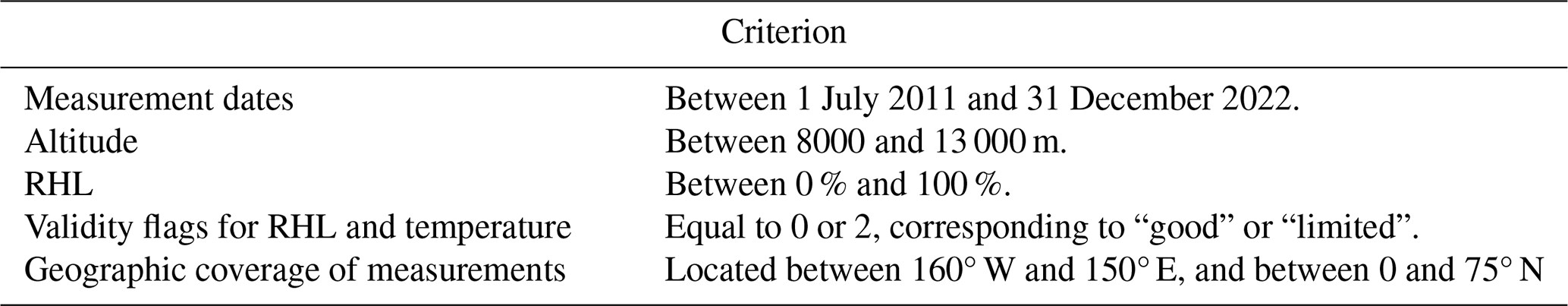
Given the start date of the IAGOS program and that the entire IAGOS fleet was equipped with the modified Vaisala HUMICAP^® of type H sensor in 2011 (Neis et al., 2015), data measured between 1 July 2011 and 31 December 2022 have been collected for the current study. The end date is set to 31 December 2022 due to a lack of published flight measurements with all observed variables after this date (at the time of data collection). The altitude is restricted between 8000 and 13 000 m as these are the flight levels that are the most visited by IAGOS aircraft. These are also the levels where we can expect ISSRs to occur in the midlatitudes (Lamquin et al., 2012; Sanogo et al., 2024). In the tropics, ISSRs are rare below 10 000 m, and have been shown to occur at altitudes of more than 15 000 m (Lamquin et al., 2012). Commercial aircraft do not cruise at such high altitudes, as also seen from the IAGOS dataset. Hence, we maintain the upper bound of 13 000 m.

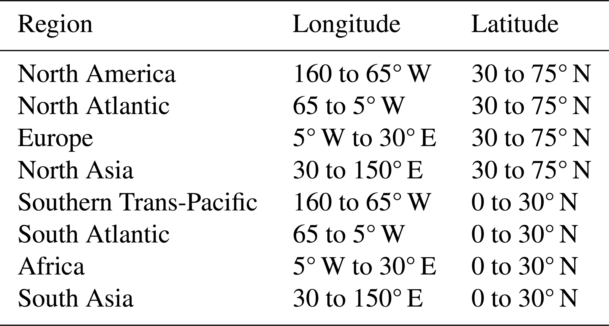
Based on the global distribution of the IAGOS measurements during the considered time frame, as seen in Fig. 1, only measurements located between 160° W and 150° E, and between 0 and 75° N will be considered. This is further divided into eight regions. The latitudes of the regions are based on the definition of extratropical (latitude < 30° S and latitude > 30° N) and tropical (30° S ≤ latitude ≤ 30° N) regions (Spichtinger and Leschner, 2016). We considered the Northern and Southern Hemisphere tropics separately due to the inter-tropical convergence zone, which causes changes in wet and dry conditions across the equator depending on its position (National Oceanic and Atmospheric Administration, 2023), as discussed in Appendix A. Due to low sampling in the Southern Hemisphere tropics, we subsequently only focus on the Northern Hemisphere. The eight defined regions are shown in Fig. 1 and have the areal boundaries given in Table 1.

Only points with a relative humidity with respect to liquid (RHL) between 0 % and 100 % are selected from IAGOS measurements. A RHL greater than 100 % implies flying through a liquid cloud, and contrails cannot form at temperatures where these clouds are present (Wilhelm, 2022).

IAGOS uses validity flags to indicate the quality of the measurements. The following validity flags are used: “good” (0), “limited” (2), “erroneous” (3), “not validated” (4) and “missing value” (7) (IAGOS, 2025e). Only “good” and “limited” measurements are considered for temperature, relative humidity with respect to ice (RHi) and RHL. However, we use the RHL validity flag to select RHi values since the quality flag of RHi was not well derived at the time of data collection, but is known to be similar to that of RHL (Sanogo et al., 2024). A summary of the criteria for the IAGOS measurements is provided in Table 2.

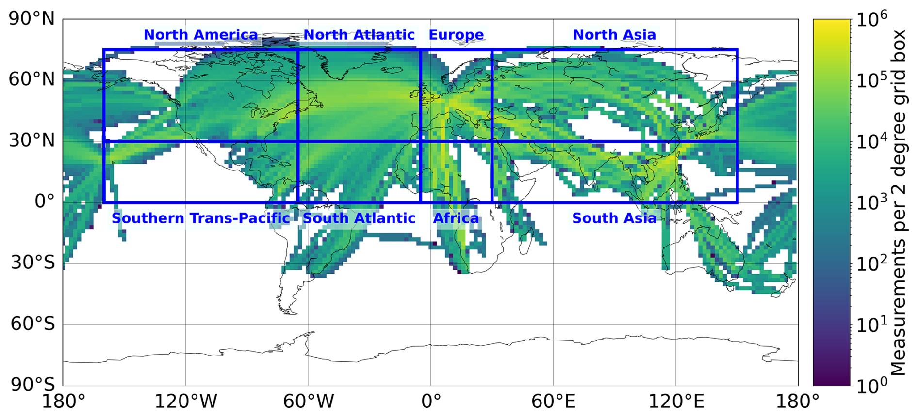
Figure 1 IAGOS measurement density map per 2° grid box with regional division between 8000 and 13 000 m from 1 July 2011 to 31 December 2022, considering “good” or “limited” validity flags for RHL and temperature.

Table 1 Areal boundaries of defined geographical regions.

Lastly, IAGOS records the measurements every four seconds. To avoid autocorrelation affecting our analysis, it is chosen to sample a measurement approximately every minute. This is done using a uniform random number generator ranging from 1 to the maximum number of measurement points from IAGOS, to avoid systematic bias. The sampling and application of the criterion from Table 2 results in using 3.8 % of all IAGOS measurements between 1 July 2011 and 31 December 2022.

Table 2 Criteria for selection of IAGOS measurements.

2.2 ERA5 reanalysis

The ERA5 reanalysis is the fifth generation reanalysis from ECMWF (Hersbach et al., 2020). To allow for a higher vertical resolution, the Analysis-Ready, Cloud Optimized (ARCO) ERA5 (Carver and Merose, 2023) has been used, which provides several atmospheric variables on model levels. ARCO ERA5 was retrieved using the python library pycontrails (Shapiro et al., 2025), which also allows for the re-gridding of model levels to pressure levels. It was chosen to re-grid with a vertical resolution of 10 hPa. This is within the range of the model level resolution at typical cruise altitudes, which is between 8 and 15 hPa when considering a surface pressure of 1013.250 hPa (ECMWF, 2025).

The ERA5 reanalysis is (quadrilinearly) interpolated in time, pressure level, longitude and latitude onto the IAGOS flight tracks using the Delftblue supercomputer (Delft High Performance Computing Centre, 2024). Since the ARCO ERA5 dataset does not provide RHi, it is derived from specific humidity, temperature and the saturation water vapour pressure over ice. The saturation water vapour pressure over ice is computed using the AERKI formula of Alduchov and Eskridge (1996) to be consistent with the ECMWF IFS formulation (European Centre for Medium-Range Weather Forecasts (ECMWF), 2016). RHi is calculated only for temperatures below 250.15 K (Hersbach et al., 2023a). However, specific humidity exhibits a nonlinear lapse rate (pycontrails, 2025). To avoid biases due to linear interpolation, RHi is therefore calculated before interpolation, where we then interpolate in the RHi space (pycontrails, 2025).

2.3 Vertical distribution of variables with respect to tropopause

The vertical distribution of the temperature, relative humidity over ice, and ISSR fraction will be reported relative to the tropopause height. Both the dynamic and thermal tropopause have been considered, and were determined using ERA5 tropospheric data reported by Hoffmann and Spang (2022). Given the stronger gradients in temperature and RHi associated with the thermal tropopause (see Appendix B), the results are presented relative to this definition. This will, for example, result in a drier lower stratosphere compared to using the dynamic tropopause definition.

The flight measurements are distributed into layers with a thickness of 30 hPa, centered at the tropopause. The selection of layers for further analysis depends on the number of data points per level, which varies per geographical region, as seen in Fig. 2. This figure shows that in the extratropic regions, the majority of measurements are distributed around the tropopause, allowing for upper tropospheric and lower stratospheric analysis. In the tropics, most of the samples are located in the upper troposphere since the tropopause is located at higher altitudes in this region.

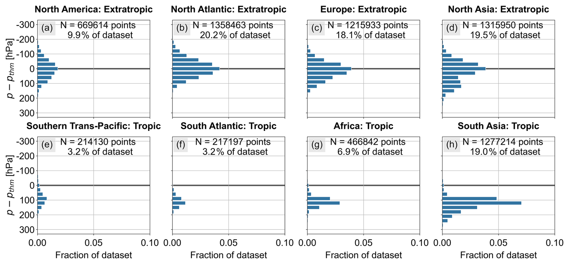
Figure 2 (a–h)Vertical distribution of number of samples with respect to distance to the thermal tropopause, p−p_thm, in different geographical regions.

2.4 Differentiation of cloudy and clear-sky conditions

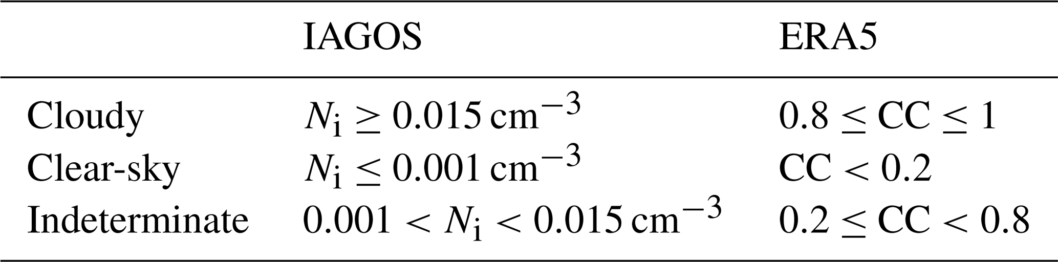
To investigate the impact of cloudy and clear-sky conditions on the ability of ERA5 to predict ISS, we need to distinguish between these two conditions. For IAGOS, the ice crystal number concentration, N_i, can be used to differentiate between measurements within cirrus clouds and within cloud-free conditions. We use the same thresholds defined by Petzold et al. (2017), which are summarised in Table 3. Indeterminate conditions refer to measurements that cannot be identified as clouds and cannot be considered cloud-free. These measurements are most likely located within very thin cirrus (Petzold et al., 2017)

For the ERA5 reanalysis, cloudy and clear-sky conditions can be differentiated using the cloud cover fraction, CC, which takes a value between 0 and 1. CC describes the proportion of a grid box covered by liquid or ice clouds (Hersbach et al., 2023a). For the analysis of RHi and ISSRs, we only consider data points where the temperature is below 235.15 K, which is below the threshold at which liquid clouds can occur (Gierens et al., 2020b), hence we focus on ice clouds. To distinguish between cloudy, clear-sky and indeterminate conditions, we use the same thresholds as Wolf et al. (2025), which are also defined in Table 3.

Table 3 Thresholds used to define cloudy, clear-sky and indeterminate conditions in IAGOS and ERA5.

The fraction of cloudy, clear-sky and indeterminate conditions, based on the definition of the ice crystal number concentration in IAGOS, per layer and geographical region, is visualised in Fig. 3. The majority of samples are categorised as no clouds or no measurements. There are few indeterminate and cloudy conditions. The low number of cloud observations is in line with reports from Sanogo et al. (2024).

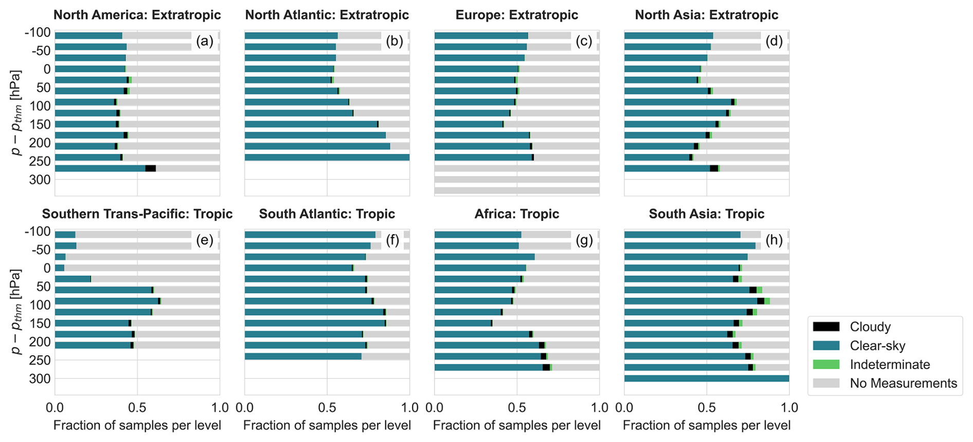
Figure 3 (a–h) Fraction of cloudy, clear-sky and indeterminate conditions per layer and geographic region, based on the ice crystal number concentration, N_i, from IAGOS measurements. No measurements means that there is no data available on the ice crystal number concentration from IAGOS.

The application of cloud cover to determine cloudy, clear-sky and indeterminate conditions using ERA5 results in the division seen in Fig. 4. We applied the “no measurements” label to ERA5 for the same points as in IAGOS.

Comparing Figs. 3 and 4, it is noticeable that there are discrepancies in the labelling of cloudy, clear-sky and indeterminate conditions between IAGOS and ERA5. We see that ERA5 shows a higher frequency of indeterminate and cloudy conditions compared to IAGOS. However, the choice of definition to use to define cloudy and clear-sky conditions in IAGOS and ERA5 largely impacts the results as shown by the sensitivity study presented in Sect. S1 of the Supplement.

Figure 4 (a–h) Fraction of cloudy, clear-sky and indeterminate conditions per layer and region, based on the definitions using the cloud cover from ERA5. No measurements means that there is no data available on the ice crystal number concentration from IAGOS, which are flagged in the ERA5 dataset as well.

3 Results

3.1 Seasonal and vertical variability of temperature between ERA5 and IAGOS

As a first step, we compare the IAGOS measured temperature and the ERA5 simulated temperature. Figure 5 shows the vertical mean temperature distribution of IAGOS and ERA5 per season, for the eight geographical regions defined. The same seasonal definition is applied for all regions to allow for a consistent comparison between the tropics and extratropics. The choice for the lower limit on the number of samples is explained in Sect. S2 in the Supplement.

The mean temperature differences in the tropical regions range between −0.25 K (ERA5 warmer than IAGOS) and 0.25 K, on average, in the upper troposphere as observed in Fig. S10 in the Supplement, which is within the IAGOS temperature sensor accuracy range. In Africa, we see mean temperature differences between 0.5 and 1 K. Furthermore, the tropics show an increased deviation between IAGOS and ERA5 close to and above the tropopause. In South Asia and Africa, the deviation causes a cold bias in ERA5, which can be attributed to the stratospheric cold bias in ERA5 (Shepherd et al., 2018). However, in the Southern Trans-Pacific, the increased deviation results in a warm bias, which may be partially explained by sensor error. In the extratropics, we find that ERA5 has a cold bias of 0.5 K on average in the upper troposphere, but it cannot be ruled out that this is due to sensor error as the mean difference is within accuracy range of the IAGOS temperature sensor. The lower stratosphere shows a slightly larger cold bias compared to the upper troposphere, with mean differences ranging from 0.75 to 1 K and can thus not be explained by sensor accuracy alone.

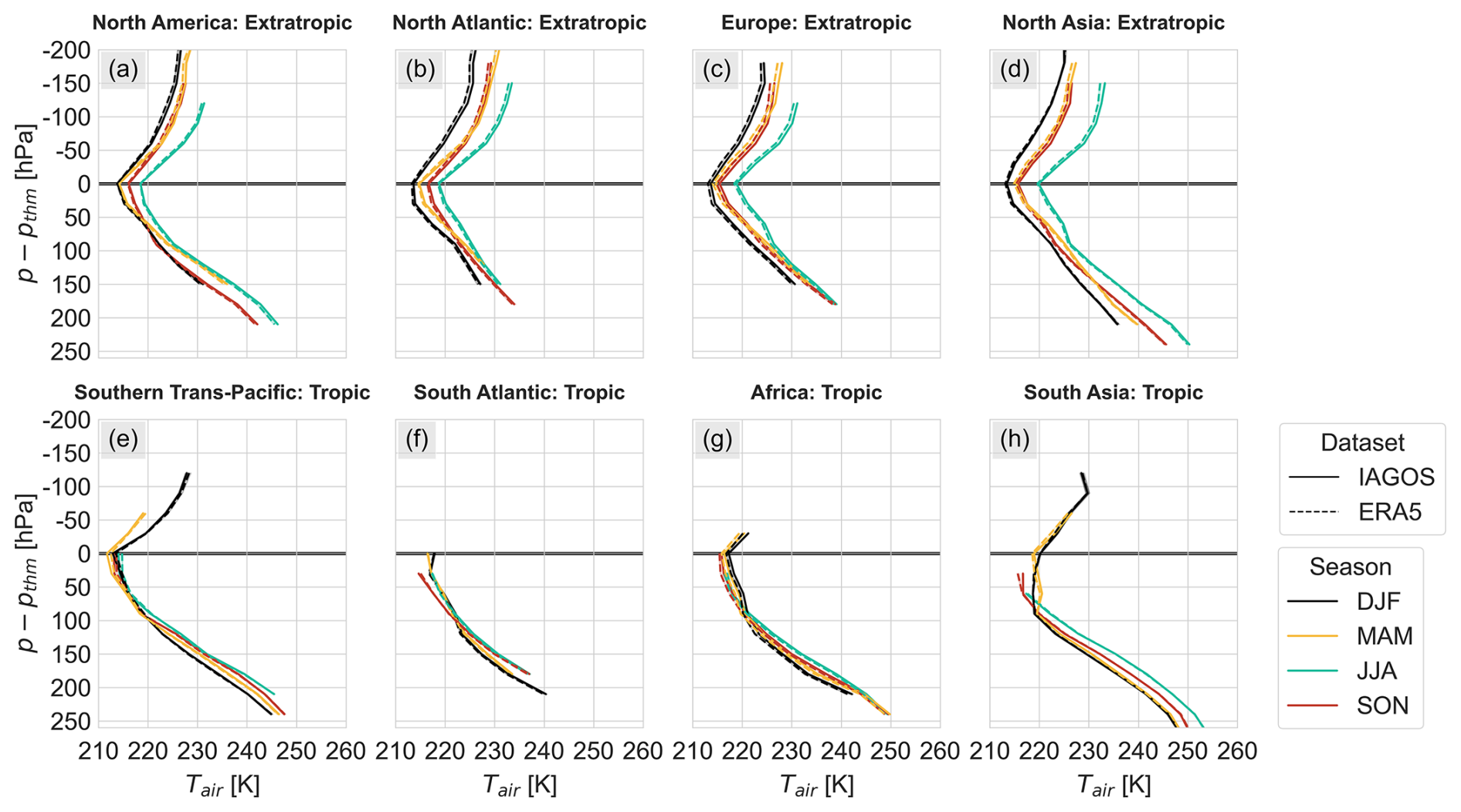
Figure 5 (a–h)Vertical distribution of IAGOS and ERA5 mean temperature per season and per region with shading showing the 95 % confidence interval, using levels based on distance to thermal tropopause, only considering levels, seasons and regions with 500+ samples.

3.2 Seasonal and vertical variability of relative humidity over ice between ERA5 and IAGOS

Ice supersaturation is governed by the RHi. We only consider RHi for cases where the temperature is below the threshold of homogeneous freezing, assumed equal to 235.15 K. This is the lowest temperature at which supercooling of cloud droplets can occur (Gierens et al., 2020b; Sperber and Gierens, 2023).

The mean vertical distribution of RHi in the IAGOS and ERA5 datasets per season and geographic region is presented in Fig. 6, using the same seasonal and regional definitions as in Sect. 3.1. In the tropics, we observe some seasonal behaviour in the Southern Trans-Pacific and in South Asia. South Asia has a larger mean RHi in season JJA compared to the other seasons in this region. The higher RHi may be the result of the tropics being a deep-convection region with strong updrafts, which result in ISS and high nucleation rates leading to a high ice crystal number concentration (Sanogo et al., 2024). Petzold et al. (2017) also found a correlation between a high ice crystal number concentration and high values of RHi. In fact, we find a higher frequency of cloudy conditions for season JJA compared to other seasons in South Asia when observing IAGOS measurements (see Fig. S12), showing that more measurements with larger ice crystal number concentrations are found in this season. Although deep convection can also happen in other tropical regions, we do not observe this due to the low sampling of in-cloud measurements with IAGOS in these regions.

For season JJA in South Asia, we also identify a moist bias in ERA5. Schneider et al. (2014) showed that the latitudinal band of 0 to 30° N, for a region covering 65 to 95° E, received the most precipitation in JJA, including September. Hence, we suggest that the moist bias may be related to the type of weather encountered in South Asia in season JJA.

In the Southern Trans-Pacific, season DJF shows an overall lower mean RHi compared to other seasons. The majority of points in this region are located close to Hawaii or Central America/northwestern South America. In North America, North Atlantic, and Europe, the highest RHi values throughout the vertical profile occur during seasons DJF and MAM, which are also the seasons that exhibit the lowest mean temperatures, as seen in Fig. 5. These are also the two seasons where we find a larger dry bias in ERA5. This is due to higher values of RHi favouring lower temperatures (Sanogo et al., 2024), and ERA5 shows more inconsistencies in the prediction of large RHi (Wolf et al., 2025). We also find that the differences between IAGOS and ERA5 appear smallest in North America and increase as we move towards Europe, showing a possible longitudinal dependency. Wolf et al. (2025) noticed the same behaviour and hypothesised it could be due to the spatial distribution of water vapour. From a global distribution of the mean RHi and ISS occurrence using IAGOS, we see that North America is drier, with less ISS occurrences, compared to the North Atlantic and Europe, which could result in larger differences in the two latter regions due larger biases in ERA5 close to and in ISS conditions (Petzold et al., 2020; Wolf et al., 2025).

In the lower stratosphere, there is a larger difference in the mean RHi between IAGOS and ERA5 compared to the upper troposphere, which can also be seen in Fig. S11 in the Supplement. This reflects the moist bias in IAGOS at low values of RHi in the dry lower stratosphere (Wolf et al., 2025). This results from the limitation of the ICH sensor; it does not provide good quality results in dry conditions in the lower stratosphere due to the loss of sensitivity as a result of the adiabatic compression effect (Konjari et al., 2025). Although the mean difference is larger in the lower stratosphere, Fig. S11 shows that the range of differences is smaller compared to the upper troposphere. This indicates that under conditions where RHi is lower, there is better agreement between IAGOS and ERA5, but the systematic moist bias in IAGOS increases the mean difference.

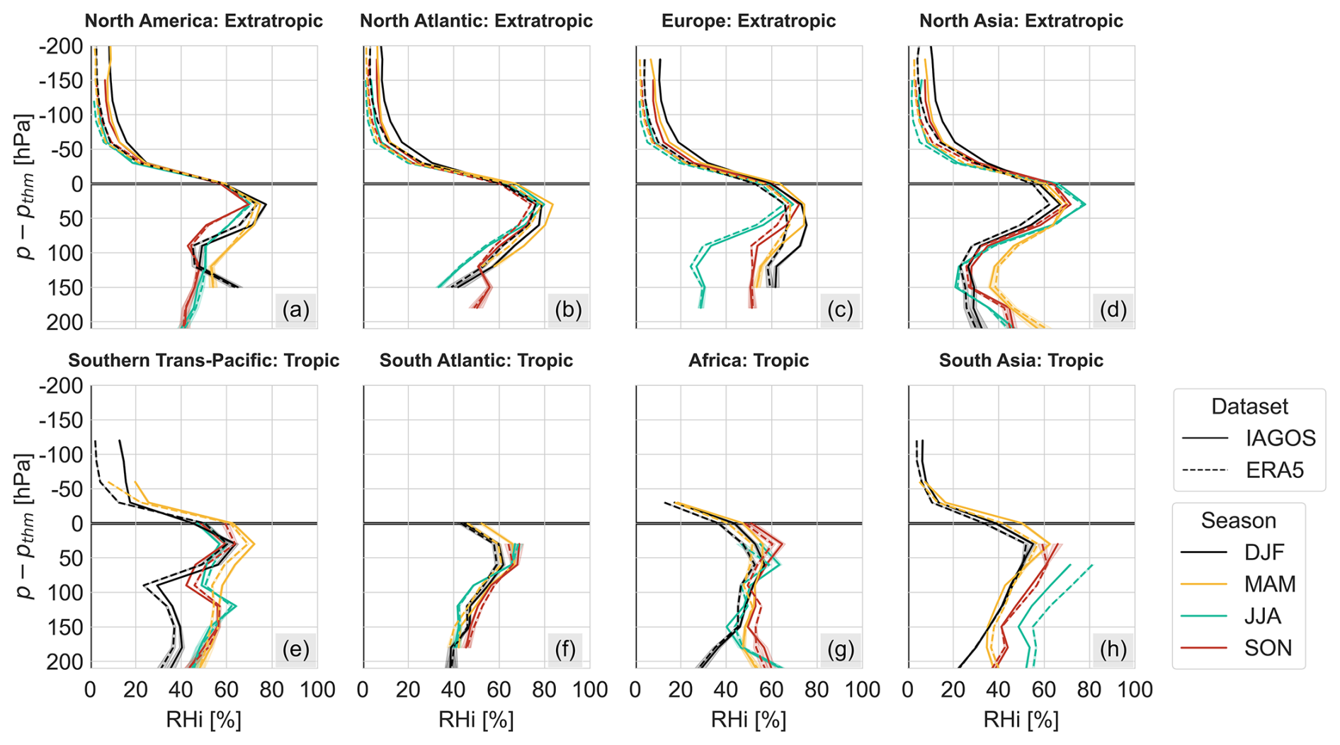
Figure 6 (a–h) Vertical distribution of IAGOS and ERA5 mean relative humidity over ice per season and per region with shading showing the 95 % confidence interval, using levels based on distance to thermal tropopause, only considering levels, seasons and regions with 500+ samples.

3.3 Distribution of relative humidity over ice from IAGOS and ERA5 under cloudy and clear-sky conditions

In this section, we investigate the effect of clear-sky, indeterminate, and cloudy conditions based on the probability density function of RHi from IAGOS and ERA5. Instead of discrete vertical levels, we consider three atmospheric layers because of the low sampling of the ice crystal number concentration in IAGOS. The three layers are upper troposphere (UT), tropopause (TROP) and lower stratosphere (LS). Their definition is based on the distance to the thermal tropopause (p−p_thm). The UT is defined as $(p-p_{\mathrm{thm}})>\mathrm{15}$ hPa, the TROP as −15 hPa $\le (p-p_{\mathrm{thm}})\le \mathrm{15}$ hPa and LS as $(p-p_{\mathrm{thm}})<-\mathrm{15}$ hPa. Note that for this analysis we consider conditions with 250+ samples instead of 500+ samples due to less measurements with ice crystal number concentration within IAGOS. However, as seen in Sect. S2 in the supplement, 250+ samples should still be sufficient.

Figures 7 and 8 display the probability density function (PDF) for the different cloudy conditions, per atmospheric layer, and per geographic region considered in this study. In the LS, we find that the extratropic clear-sky PDF is governed by low values of RHi and a general monotonically decreasing behaviour. The IAGOS measurements show that ISS is possible in the LS, but the probability of occurrence is low. Meanwhile, ERA5 shows little to no ISS occurrence under clear skies in the extratropics. In the tropic regions, the clear-sky PDF in the LS shows some multimodal behaviour, but this is likely the result of a small number of samples in this atmospheric layer due to the high altitude of the tropopause in these regions (see Fig. 2). Here, the probability of ISS conditions is much more rare compared to the extratropics. However, we do observe a low probability of ISS conditions in South Asia.

Both the extratropics and tropics show small differences in low values of RHi in the LS under clear-sky conditions. This is not necessarily due to biases in ERA5, but may be due to limitations of the IAGOS ICH sensor as discussed in Sect. 3.2. However, this will not impact the prediction of ice supersaturated regions as the issue only arises below RHL ≈ 10 % (Konjari et al., 2025), which is equivalent to RHi ≈ 15 %–18 % given the mean temperature in the LS.

The UT has more moisture compared to the TROP and LS, allowing for higher probabilities of ISS occurrence. However, the TROP also shows high ISS occurrence, both in the tropics and extratropics. This is in line with Reutter et al. (2020), where it was found that there was a significant amount of in situ and ERA-interim data that exceeded the RHi = 100 % threshold near the tropopause in the North Atlantic flight corridor. For UT and TROP clear-sky conditions, the probability of RHi >100 % is higher and there is a more uniform probability across the observed RHi range compared to the LS. ERA5 shows good approximation of RHi below ISS in UT and TROP clear-sky conditions until RHi ≈ 85 %–90 %, with a drop-off in probability just before RHi=100 %. The underestimation of ISS in ERA5 for clear-sky conditions may be the result of the resolution of ERA5, which only provides hourly mean and grid cell values (Schumann et al., 2021). However, it shows that by lowering the threshold value of RHi for ISS, we could artificially increase the prediction of ISS in ERA5, though the value may differ per region; as seen from Fig. 7, the RHi threshold value would be close to 100 % for North America, but it might be closer to 85 % in Europe.

Cloudy and indeterminate conditions in ERA5 for the UT and TROP are governed by narrow peaks centred around RHi=100 % due to the saturation adjustment. For IAGOS, these peaks are centred at higher values of RHi, with wider distributions as cirrus clouds often exhibit an ice supersaturated wet mode, but they can also be subsaturated (Sanogo et al., 2024). In South Asia, we find that this mode is subsaturated in the UT in the IAGOS measurements. This observation in South Asia may also provide insights into the moist bias found in JJA (Sect. 3.2). The mean vertical distribution of RHi shows a higher mean RHi for ERA5 compared to IAGOS in cloudy and indeterminate conditions for South Asia in JJA, at vertical levels below the tropopause. This is because the mean RHi in IAGOS for this particular region and season is less than 100 % in cloudy and indeterminate conditions, which aligns with the behaviour of the RHi PDF, whereas ERA5 shows a mean of 100 %. Therefore, the moist bias appears to arise because ERA5 cannot take into account that the wet mode in cloudy conditions can be subsaturated in some regions. Whether the subsaturation is a result of the specific weather conditions in JJA in South Asia is uncertain and requires further evaluation.

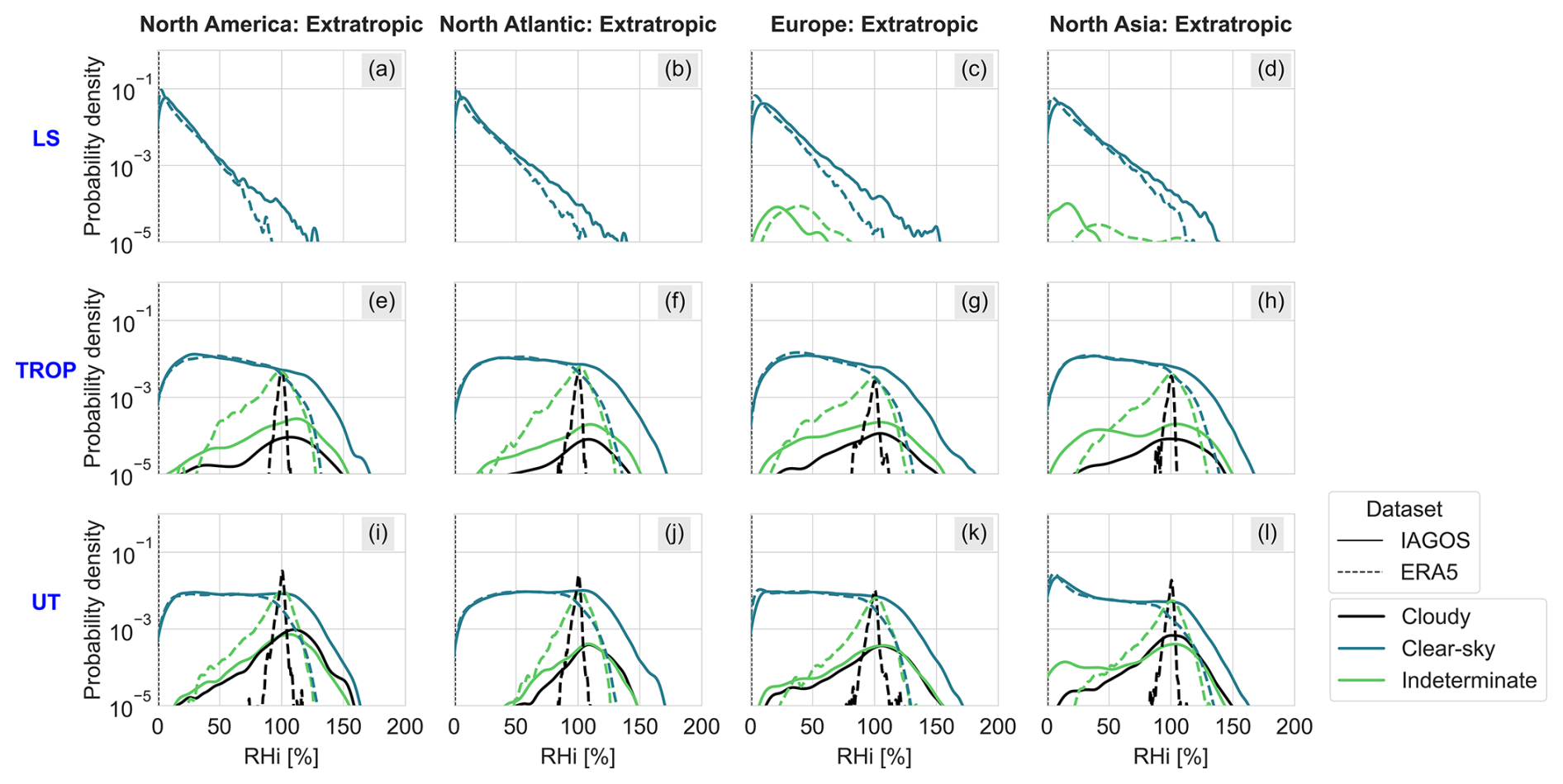
Figure 7 (a–l) Probability density function of IAGOS and ERA5 relative humidity over ice in the upper troposphere (UT), at the tropopause (TROP) and in the lower stratosphere (LS) for cloudy, clear-sky and indeterminate conditions in the four extratropic regions. The PDFs per subplot are normalised with respect to the number of observations within each subset of IAGOS or ERA5 used for that subplot. Only regions and atmospheric layers with 250+ samples are considered.

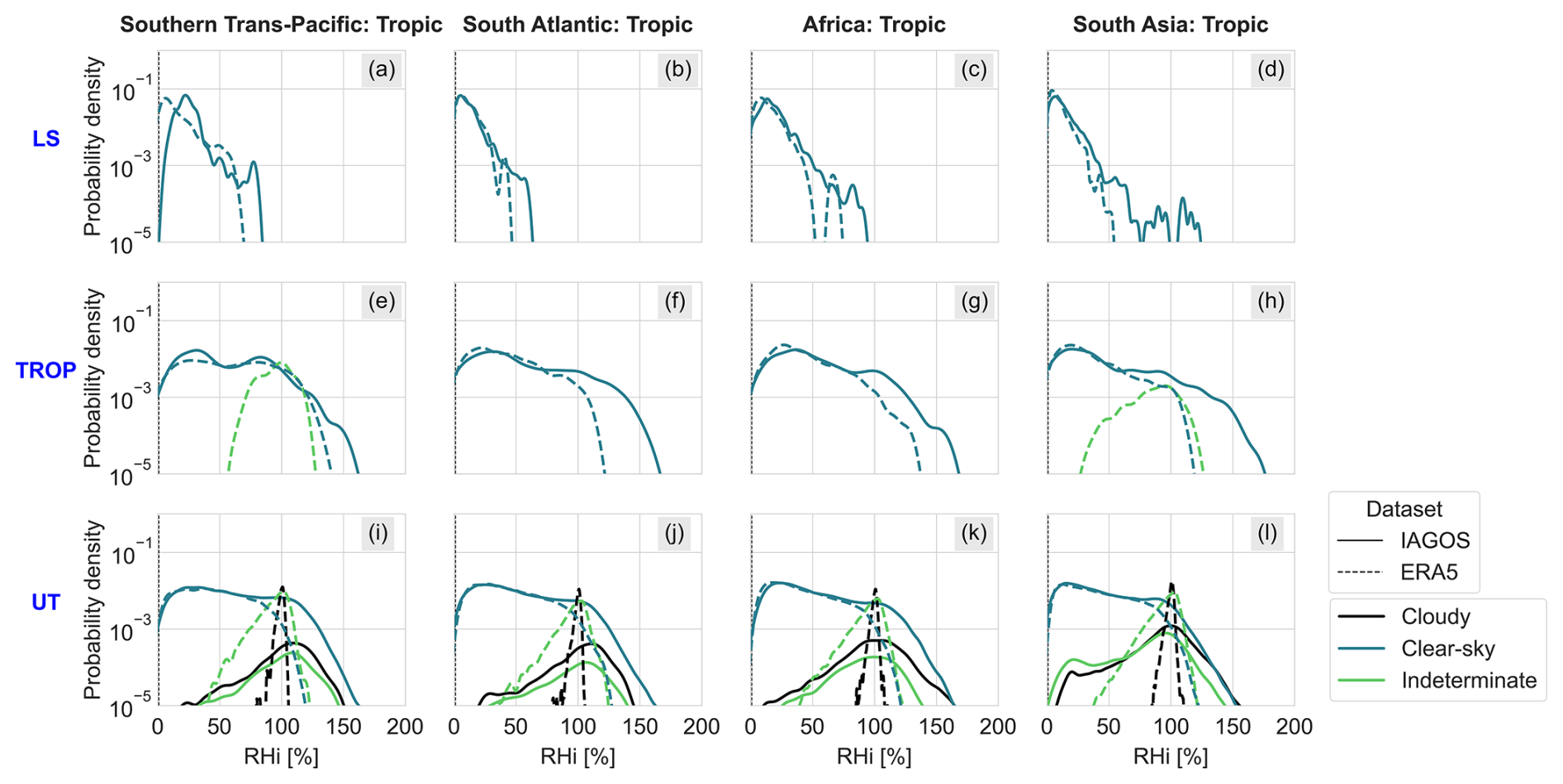
Figure 8 (a–l) Probability density function of IAGOS and ERA5 relative humidity over ice in the upper troposphere (UT), at the tropopause (TROP) and in the lower stratosphere (LS) for cloudy, clear-sky and indeterminate conditions in the four tropic regions. The PDFs per subplot are normalised with respect to the number of observations within each subset of IAGOS or ERA5 used for that subplot. Only regions and atmospheric layers with 250+ samples are considered.

3.4 Distribution of ice supersaturated regions in ERA5 and IAGOS

Comparison of the RHi showed a general dry bias in ERA5, compared to IAGOS, with some seasonal and regional differences. In the following section, we will explore the impact of such biases on the ice supersaturated region occurrence.

Figure 9 displays the vertical distribution of the ISSR fraction per season and geographical region. The ISSR fraction is calculated by finding the total number of points showing ISS conditions and dividing by the total number of points, per vertical level, season and geographical region. There is an overall underestimation of ISSRs in ERA5 due to the dry bias in RHi. In instances where the RHi is overestimated by ERA5, such as in South Asia for season JJA, the ISSR fraction is overestimated by ERA5.

In the tropics, we generally report an increasing ISSR fraction up to just below the tropopause, with a maximum of 20 %. The South Atlantic, Africa, and South Asia show little seasonal dependence. In the Southern Trans-Pacific, it is observed that the maximum ISSR fraction in the Southern Trans-Pacific occurs closer to the tropopause in DJF than in JJA. The vertical profile of the mean RHi in DJF for this region also showed a more pronounced increase near the tropopause compared to other seasons (see Fig. 6). In the layer between 100 and 200 hPa below the tropopause, the ISSR fraction in DJF is lower than in the other seasons, which is consistent with the lower mean RHi in this layer.

For South Asia, we do not find that the ISSR fraction is higher in JJA in the IAGOS measurements, despite the higher overall mean RHi. This could be related to the higher frequency of cloudy conditions in South Asia in JJA, for which the wet mode of the RHi PDF is subsaturated, leading to less ISS occurrences. ERA5 shows a higher ISSR fraction throughout the vertical profile in JJA; this was also the season for which ERA5 showed a moist bias. Otherwise, we find no distinct seasonal behaviour in the tropics.

There is a clear seasonal pattern in North America, North Atlantic and Europe, with DJF and MAM showing the highest ISSR occurrence. For these seasons, IAGOS shows maximum ISSR fractions between 30 % and 35 % with IAGOS, typically occurring just below the tropopause (around 30 hPa, ≈ 750 m at cruise level; Thouret et al., 2006; Petzold et al., 2020) and decreases to zero in the lower stratosphere.

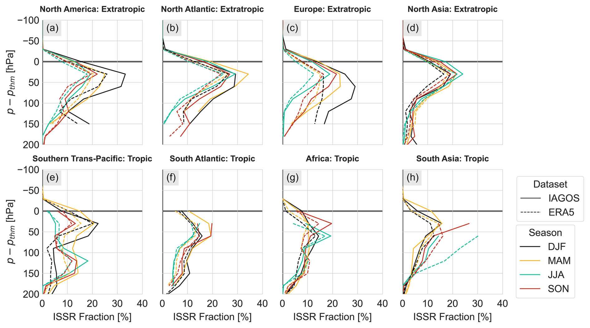
Figure 9 (a–h) Vertical distribution of IAGOS and ERA5 ice supersaturated region fraction per season and geographical region. Only levels, seasons and regions with 500+ samples are considered.

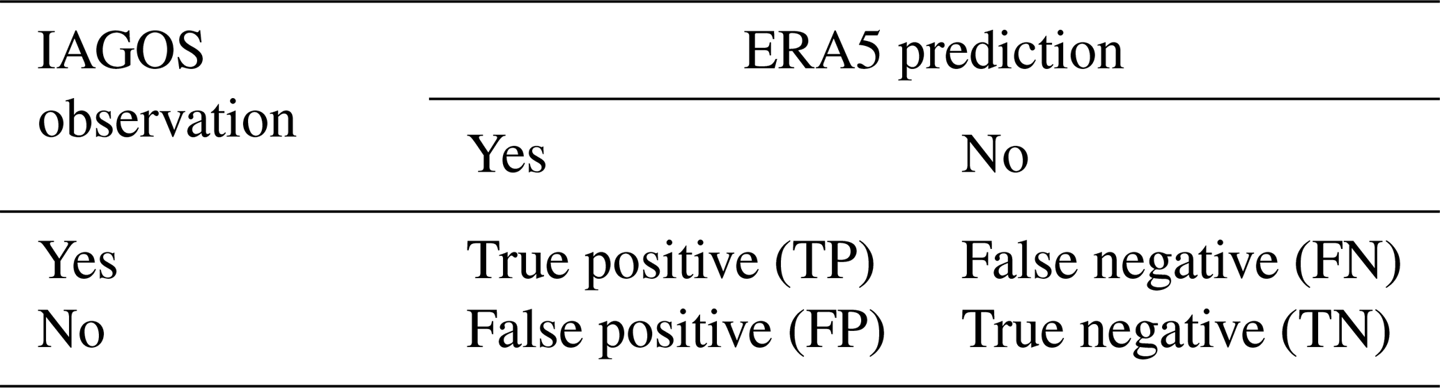
To quantify the skill of ERA5 in predicting ISSRs, we can use the equitable threat score (ETS). This performance measure is preferred over measures such as the hit rate and false alarm rate since ISSRs can be a rare event (Gierens et al., 2020a; Wolf et al., 2025), for example in the lower stratosphere. The ETS is calculated using Eq. (1), where r is found with Eq. (2) and the other variables are entries in the contingency table shown in Table 4. If ETS=1, there is a perfect correlation between the observation and the prediction (Gierens et al., 2020a). When ETS=0, the relationship is completely random (Gierens et al., 2020a). We investigate how the ETS varies with different RHi thresholds in ERA5, while keeping the threshold of 100 % in IAGOS.

$$\begin{array}{}\text{(1)}& {\displaystyle }\text{ETS}={\displaystyle \frac{\text{TP}-r}{\text{TP}+\text{FN}+\text{FP}-r}}\text{(2)}& {\displaystyle }r={\displaystyle \frac{(\text{TP}+\text{FN})(\text{TP}+\text{FP})}{\text{TP}+\text{FN}+\text{FP}+\text{TN}}}\end{array}$$

Figures 10 and 11 show the vertical distribution of the ETS per geographical region for different ERA5 RHi thresholds in DJF and JJA, respectively. When using the threshold of RHi=100 %, the ETS lies between 0.2 and 0.4 in the upper troposphere, depending on the season, vertical distance to the tropopause and region. This means that there is a weak to mediocre correlation between IAGOS and ERA5 in the prediction of ISSRs. There are a few instances of high ETS scores: North America in season JJA at 180 hPa below the tropopause and North Atlantic in season DJF at 150 hPa below the tropopause. For North America in season JJA at 180−p_thm hPa, there is a low number of ISSRs in both IAGOS and ERA5 (see Fig. 9), where one measurement point is classified as TP, one point as FN and the rest as TN. Since the ISSR events are rare, resulting in a perfect hit rate, accompanied with most points classified as TN, the ETS can inflate. We see a similar low ISSR fraction for North America in season JJA at 150−p_thm hPa, although the ETS is not as high. This can be attributed to more points being categorised as FN and FP, lowering the ETS. In the North Atlantic, in season DJF at 150 hPa below the tropopause, we also find a high ETS. In the instances where an ISSR is observed here, most of these events are classified as TP, with no misses (FN = 0), and there were few points classified as FP compared to TP. At the same time, there are also many points classified as TN. The combination of this leads to a high ETS.

Table 4 Contingency table definition.

By reducing the RHi threshold, we can improve the ability of ERA5 to predict ISSRs, as shown by the ETS. The optimal RHi thresholds are in the range of 85 % to 95 % in the upper troposphere and in the tropopause. However, it is also dependent on the region, distance from the tropopause and the season, but a clear pattern is difficult to establish. In the extratropics, more improvements in the ability of ERA5 to predict ISSRs can be achieved in DJF by reducing the RHi threshold compared to in JJA. This could be due to lower RHi values and thus less ISSRs in warmer months, such as JJA, although North Asia shows the highest ISSR fraction for this season, as seen in Fig. 9. SON and MAM also show more improvements compared to JJA when lowering the RHi threshold (see Sect. S5 in the Supplement). Overall, only a certain improvement can be achieved by changing the RHi threshold. Not accounting for the outliers, we observe that we cannot achieve an ETS higher than approximately 0.5 in DJF and around 0.3 in JJA in the upper troposphere and in the tropopause.

In the extratropic lower stratosphere, lowering the RHi threshold in ERA5 shows a minor improvement in the ETS, but the ETS score still indicates a weak correlation between IAGOS and ERA5. There is a low number of ISSR occurrences in this layer, which combined with the underestimation of RHi in ISS conditions, might make it difficult for ERA5 to predict ISSRs in these instances, resulting in a low ETS.

In the tropics, DJF also shows larger ETS improvements by decreasing the RHi threshold compared to other seasons in the upper troposphere. It is also interesting to note that in South Asia in JJA, where we observed a moist bias in ERA5, both increasing and decreasing the RHi threshold in ERA5 has little to no impact on the ETS. This could be the result of a higher frequency of cloudy conditions in this particular season, for which changing the RHi threshold may not have a large effect. In Southern Trans-Pacific, we find that ERA5 shows better prediction of ISSRs when lowering the RHi threshold in DJF, compared to in JJA, MAM and SON, with SON showing the lowest ETS. SON has the highest fraction of cloudy conditions and DJF the lowest. The effect of cloudy conditions on the ETS with different RHi thresholds will be analysed further in the following section.

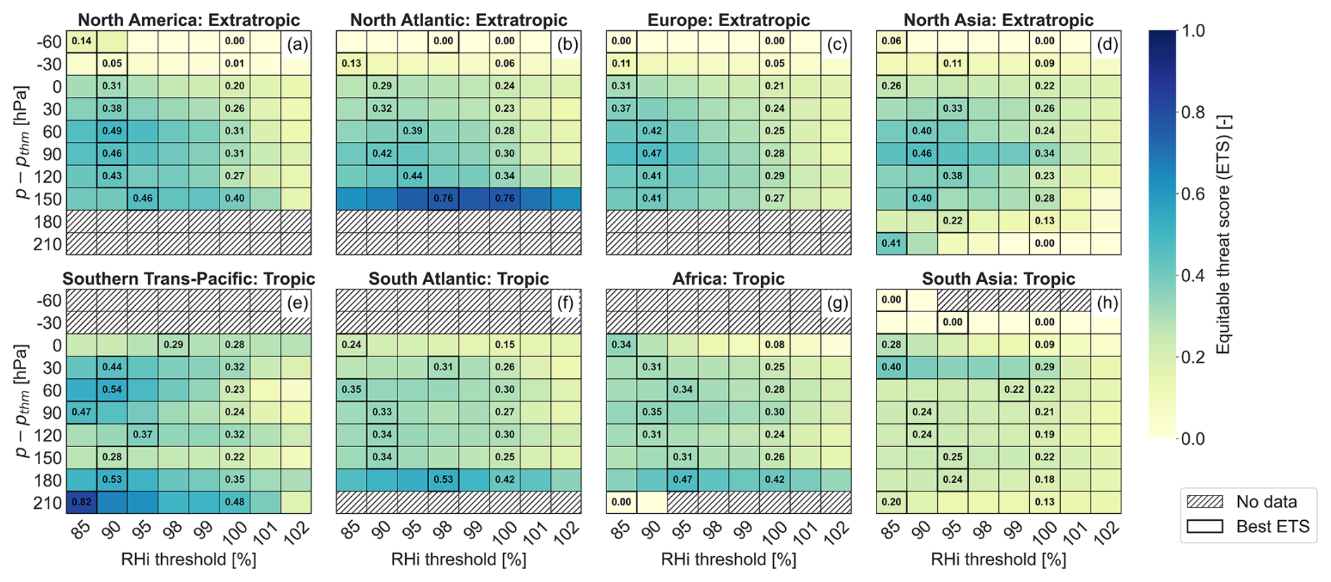
Figure 10 (a–h) Vertical distribution of ice supersaturated region equitable threat score per geographical region for different ERA5 RHi thresholds in DJF. For each level, we highlight the ETS for a threshold of 100 % and the ETS for the threshold at which we find the maximum value. ETS is calculated for level, season and region for which there are 500+ samples.

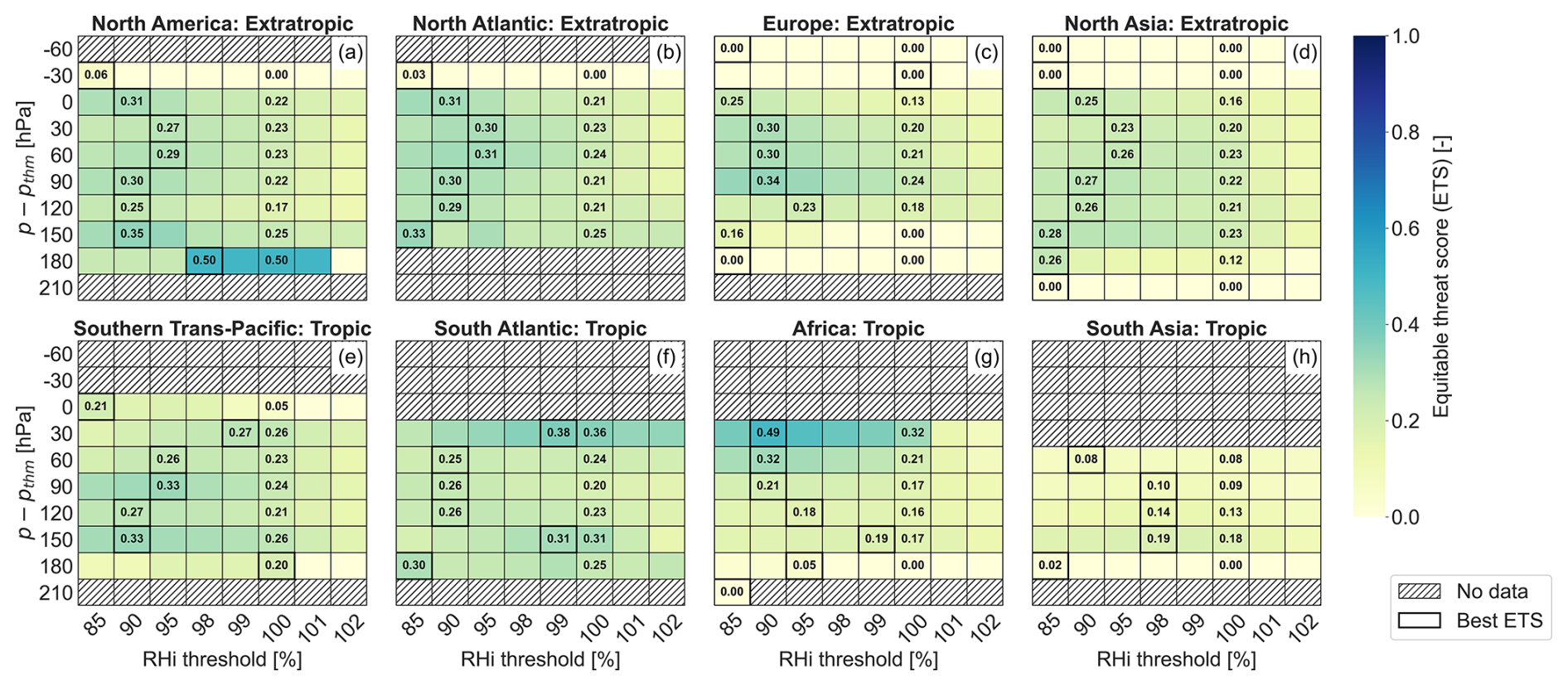
Figure 11 (a–h) Vertical distribution of ice supersaturated region equitable threat score per geographical region for different ERA5 RHi thresholds in JJA. For each level, we highlight the ETS for a threshold of 100 % and the ETS for the threshold at which we find the maximum value. ETS is calculated for level, season and region for which there are 500+ samples.

3.5 Prediction of ice supersaturated regions in ERA5 under cloudy and clear-sky conditions

In Sect. 3.3, the effect of cloudy conditions on the RHi was investigated for the different atmospheric layers and for the different geographical regions. Here, we explore the effect of cloudy and clear-sky conditions on the capability of ERA5 to correctly identify ice supersaturated regions, and the effect of varying the RHi threshold in ERA5. Again, we only consider the three atmospheric layers due to low sampling of the ice crystal number concentration in IAGOS, as described in Sect. 3.3.

Figures 12 and 13 display the ETS for clear-sky and cloudy conditions for different ERA5 RHi thresholds. In clear-sky conditions, we find an ETS of approximately 0.15 in the extratropic UT and TP. This indicates a weak coherence in the prediction of ISSRs between IAGOS and ERA5 and is the result of the clear-sky dry bias in ERA5 discussed in Sect. 3.3. The ETS reduces to between 0 and 0.05 in the clear-sky LS due to the rare occurrence of ISSRs and the underestimation of ISSRs by ERA5. For cloudy conditions, the ETS is between 0.05 and 0.08 in most extratropic regions, indicating an almost purely random relationship between IAGOS and ERA5, which is most likely resulting from the saturation adjustment in the IFS. In North America, we find the ETS in the cloudy UT to be 0.14, showing a weak coherence. No ETS are calculated in the extratropic TP or LS under cloudy conditions due to insufficient samples.

In the tropics, the ETS is generally 0.05 in the clear-sky UT and show little increase or decrease in the TP when considering the RHi = 100 % threshold. In the cloudy UT, the tropics shows an ETS of 0.1 or less, showing an almost entirely random relationship. The lower ETS in the tropics is also inline with the results presented in Sect. 3.4 and shows that ERA5 has little to no skill in predicting ISSR occurrence in tropic regions.

We find that by lowering the ERA5 RHi threshold, we can improve the predictive skill of ERA5 under clear-sky conditions. In the extratropics, a threshold of 85 % shows the best ETS in the UT and TROP, although the increase is only approximately 0.1. In the extratropical LS, decreasing the RHi threshold to 85 % results in only a marginal ETS improvement due to the low overall occurrence of ISSRs, with scores indicating a weak relationship. Similarly, in the tropical UT and TP, we find that the ETS increases by 0.1 on average when reducing the ERA5 RHi threshold to 85 % under clear-sky conditions.

Reducing the ERA5 RHi threshold under cloudy conditions in North America and North Asia also allows for minor improvements in the prediction of ISSRs in ERA5. In the North Atlantic and Europe, the best threshold appears to be 99 %, without showing much improvement in the ETS. In the North Atlantic, the hit rate and false alarm are both high at the threshold of 100 %. As the RHi threshold is decreased, both the hit rate and false alarm increase such that they are almost equal, while lowering the ETS. We see a similar occurrence in Europe; the difference is that the false alarm rates are lower, resulting in an ETS that is higher than in the North Atlantic. While this also occurs in North America and North Asia, the increase in the false alarm rate with the decrease in RHi threshold is not as high as in the North Atlantic or in Europe. The same reasoning also applies to the tropical regions. Hence, while lowering the RHi threshold does increase the number of correctly predicted ISSRs in ERA5, it comes at the cost of more false positives.

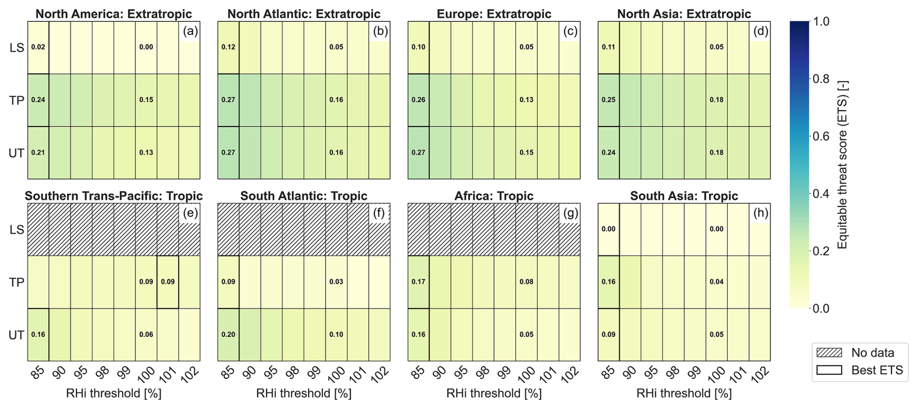
Figure 12 (a–h) Ice supersaturated region equitable threat score under clear-sky conditions for different ERA5 RHi thresholds in the upper troposphere (UT), tropopause (TP) and the lower stratosphere (LS). The different conditions have been matched between IAGOS and ERA5. Only combinations with 250+ samples are considered. For each layer, we highlight the ETS for a threshold of 100 % and the ETS for the threshold at which we find the maximum value.

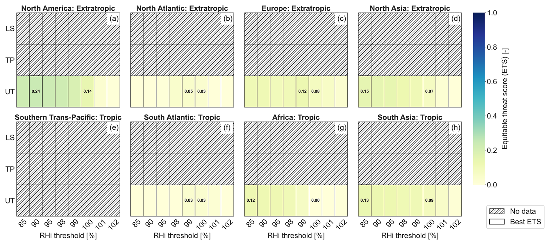
Figure 13 (a–h) Ice supersaturated region equitable threat score under cloudy conditions for different ERA5 RHi thresholds in the upper troposphere (UT), tropopause (TP) and the lower stratosphere (LS). The different conditions have been matched between IAGOS and ERA5. Only combinations with 250+ samples are considered. For each layer, we highlight the ETS for a threshold of 100 % and the ETS for the threshold at which we find the maximum value.

4 Discussion

The results presented in this paper largely agree with other studies. The extratropical upper tropospheric cold bias of 0.5 K in ERA5 compared to IAGOS is in line with Wolf et al. (2025), who compared ERA5 and IAGOS in the mid-latitudes at different pressure levels. The observed extratropical lower stratospheric cold bias in ERA5 compared to IAGOS of 0.75–1 K aligns with results from Shepherd et al. (2018), who reported a cold bias of up to 0.5 K in comparison to radiosondes in the lower stratosphere of ERA5 due to an underlying cold bias in the IFS. The vertical distribution of RHi using IAGOS measurements in the extratropics is similar to that reported by Petzold et al. (2020). The ERA5 extratropical dry bias is in line with other studies (Reutter et al., 2020; Wolf et al., 2025). We also observed a lower RHi from ERA5 than IAGOS in the lower stratosphere, but we cannot ascertain that it is due to biases in ERA5. In fact, some studies have also reported a general moist bias in the lower stratosphere in the ECMWF-IFS (Dyroff et al., 2014; Shepherd et al., 2018; Bland et al., 2021).

The overall behaviour of the RHi PDF under cloudy, clear-sky and indeterminate conditions in the UT and TROP is similar to that found by Wolf et al. (2025), but we find larger difference in the peak probability between IAGOS and ERA5 for cloudy and indeterminate conditions. If we consider the same geographic area, pressure levels and time frame for IAGOS measurements as Wolf et al. (2025) and do not consider separate atmospheric layers and do not normalise given the number of observations, we obtain more similar results to Wolf et al. (2025). We also found a low probability of RHi > 100 % in the lower stratosphere using IAGOS measurements, which was also reported by Gierens et al. (1999) using the global distribution of MOZAIC flights and by Sanogo et al. (2024) in high-latitude regions (60–80° N) using IAGOS measurements. In South Asia, we also found that the wet mode was subsaturated using IAGOS measurements. Sanogo et al. (2024) found similar observations when considering a larger tropical region.

In terms of the ISSR fraction, we observed that the ISSR fraction in the tropics increased up to just below the tropopause, and reached a maximum of 20 % when looking at IAGOS. This is similar to Sanogo et al. (2024), who reported a maximum ISSR fraction of 15 % in the tropics using IAGOS; the ISSR frequency varied about 5 % or less among the four considered seasons in the tropics. Lamquin et al. (2012) also observed increasing ISSR occurrence with altitude in the tropics using MOZAIC, with maximum ISSR frequencies of up to 30 %, but this study considered the frequency per individual grid box. The vertical structure of the ISSR fraction found using IAGOS measurements in the extratropics is also consistent with earlier findings (Petzold et al., 2020; Reutter et al., 2020; Sanogo et al., 2024), but we observe some variance in the maximum ISSR fraction reported with IAGOS/MOZAIC. A maximum ISSR fraction of 40 % was found when considering all seasons (Reutter et al., 2020) and 20 % in the midlatitudes for DJF and MAM (Sanogo et al., 2024). However, the ISSR fraction is sensitive to the number of samples and these studies use different subsets of the IAGOS/MOZAIC dataset.

We also found that the ISSR fraction is generally underestimated by ERA5 due to the observed dry bias. Reutter et al. (2020) observed the same for ERA-interim when considering the North Atlantic region. As expected, when the RHi is overestimated by ERA5, such as in South Asia for season JJA, the ISSR fraction is overestimated by ERA5 as well. Agarwal et al. (2022) found a tendency for ERA5 to overestimate the ISSR occurrence at cruise altitudes in the tropics and mid-latitudes when compared to radiosonde measurements. However, the radiosonde measurements are not corrected for dry biases and the location of these radiosonde observations are generally over land and not very widespread as with the IAGOS measurements, which could lead to differences in obtained results.

Gierens et al. (2020a) calculated ETS between 0.05 and 0.25, depending on the season. The value of 0.05 is on the lower side compared to the results in Sect. 3.4, but this may be because the study does not take into account the different atmospheric layers or regions, and it also only considers four months of IAGOS measurements. If we do not take into account the vertical layers defined, the ETS remains between 0.15 and 0.3. Hence, the low ETS found by Gierens et al. (2020a) is most likely the result of using a smaller subset of IAGOS and ERA5 data. The study by Wang et al. (2025) shows an ETS of 0.23 upper troposphere (UT) and 0.14 in the lower stratosphere before application of the machine learning algorithm, which agrees well with the values identified in this study.

We find different ETS scores in clear-sky and cloudy conditions compared to Wang et al. (2025), who found an ETS score of 0.06 in clear-sky upper troposphere and lower stratosphere (UTLS). In the cloudy UTLS, Wang et al. (2025) calculated an ETS score of 0.23. These different ETS scores are the result of using different methodologies for classifying cloudy and clear-sky conditions. Wang et al. (2025) uses the specific cloud ice water content from ERA5 to determine if a point is within a cloud or in clear-sky. Other papers use the ice crystal number concentration to determine cloudy conditions in IAGOS measurements (Petzold et al., 2017; Sanogo et al., 2024; Wolf et al., 2025), but the reporting of cloudy conditions compared to ERA5 appears relatively new. Only Wolf et al. (2025) and Wang et al. (2025) seem to have considered such a comparison, but use different variables to determine in-cloud conditions in ERA5. As discussed in Sect. S1 in the Supplement, the cloud ice water content definition tends to classify measurements as in-cloud even in the presence of subvisible cirrus. This reduces the number of points classified as clear-sky and, consequently the observable ISSR occurrence in these conditions. However, for contrail avoidance purposes, distinguishing between clear-sky and subvisible cirrus is not critical as contrail cirrus would result in a warming impact in both cases (Petzold et al., 2025). Hence, maintaining the ice crystal number concentration from IAGOS as the observational reference, we recommend using the cloud cover in ERA5 to distinguish between cloudy and clear-sky conditions.

In an attempt to identify when biases in ERA5 might arise and how to correct them, we recommend as future research to explore the correlation between weather pattern and the ability of ERA5 to estimate ISSRs. As an example, we explored whether the type of North Atlantic weather pattern can affect the observed biases in ERA5 since Irvine et al. (2012) found that the probability of forming contrails as a function of altitude depends on the weather patterns when using ERA-Interim. The methodology is explained in the Supplement (Sect. S7). The variability of ERA5 biases under the five winter weather patterns was found to be larger than the one under the three summer weather patterns. For the winter weather patterns, we see more distinct weather dependency of the biases on eastbound routes compared to on westbound routes. We suggest that this could be due to the variability of the jet stream location and strength, which determines the distribution of ISSRs, although the interpretation of these findings requires further investigation.

Another factor influencing our conclusions is the availability of IAGOS measurements. Without enough measurements, our conclusions may not be representative. Therefore, we evaluated the necessary number of points needed to be confident in our results (see Sect. S2 in the Supplement). Nevertheless, there are still some limitations. In our evaluation on the prediction of ISSRs in ERA5 under cloudy and clear-sky conditions, we lowered the minimum sample size required for a representative result due to low sampling of the ice crystal number concentration in IAGOS. This results in a larger variability of the ETS, and thus the true value may be higher or lower than reported, though, the 95 % confidence interval lies close to the mean of 100 tests. For future work, it would be helpful to increase the number of IAGOS aircraft capable of measuring the ice crystal number concentration to further distinguish between cloudy and clear-sky conditions.

5 Conclusions

In this study, we evaluated ERA5 temperature, relative humidity over ice (RHi) and ice supersaturated region (ISSR) occurrence against IAGOS in situ measurements over the period 2011–2022. Differences in the frequency of ice supersaturation (ISS) were also compared. The analysis was performed over a large geographical area covering the tropics and extratropics. It included the upper troposphere (UT) and lower stratosphere (LS), with vertical levels defined based on distance to the thermal tropopause. The RHi and ISSR occurrence is also documented for cloudy and clear-sky conditions. We used the ice crystal number concentration in the IAGOS measurements and the cloud cover in ERA5 to distinguish between cloudy, clear-sky and indeterminate conditions. The impact of changing the ERA5 RHi threshold on the ability of ERA5 to predict ISSRs was also investigated. The main conclusions of our study are as follows:

1. The vertical distribution of temperature and relative humidity over ice was analysed per season and region for IAGOS and ERA5. Temperature differences between IAGOS and ERA5 were mainly a function of the atmospheric layer, with a larger cold bias in the LS. ERA5 showed a dry bias in RHi for all atmospheric layers, but the differences in the lower stratosphere may be due to limitations of the IAGOS ICH sensor. Larger dry biases were found in colder months in the extratropics due to larger values of RHi occurring in these conditions. A moist bias was identified in South Asia for season JJA.

2. We characterised the PDF of RHi in the UT, the tropopause (TROP) and the LS for cloudy, clear-sky and indeterminate conditions. In clear-sky conditions, ERA5 showed an underestimation of ISS. In cloudy conditions, ERA5 displayed large peaks centred at RHi=100 %, due to the scheme that lowers RHi to saturation when clouds are present (saturation adjustment). This is more critical in the UT and TROP, since the LS is dry and cloud occurrence is rare, with little to no ISS conditions. While this generally also results in a dry bias, it can also cause a moist bias if the wet mode of the RHi PDF is subsaturated.

3. ERA5 showed a general underestimation of ISSRs in comparison to IAGOS due to biases in the RHi. The ability of ERA5 to predict ISSRs was estimated using the equitable threat score (ETS). With an RHi threshold of 100 %, ERA5 shows a weak to mediocre correlation with IAGOS. We found that the ability of ERA5 to predict ISSRs can be improved by decreasing the ERA5 RHi threshold. The optimal value ranges between 85 % to 95 % in the upper troposphere and tropopause, and it shows a dependency on the region, distance from the tropopause and the season, with more improvements possible in DJF compared to JJA. However, the improvement is limited, as ETS values do not exceed about 0.5 in DJF and 0.3 in JJA. In the lower stratosphere, RHi threshold adjustments have little effect on the predictive skills of ERA5.

4. The ETS for various ERA5 RHi thresholds was also calculated for the prediction of ISSRs under cloudy, clear-sky and indeterminate conditions. It showed a better coherence between IAGOS and ERA5 for clear-sky conditions compared to cloudy conditions, particularly in the extratropics. Better predictive skills of ERA5 can generally be achieved by lowering the RHi threshold to 85 %, albeit the improvements are limited and ERA5 still exhibits a weak to mediocre correlation with IAGOS. The ETS values for cloudy conditions indicate an almost random relationship. Improvements from lowering the RHi threshold are constrained by the resulting increase in false alarms.

This study is an extension of previous studies comparing IAGOS and ERA5, such as Gierens et al. (2020a) and Wolf et al. (2025). These studies also find ERA5 to underestimate ISSR occurrence compared to in situ measurements due to biases in estimation of RHi in ERA5. However, they are limited in their regional and seasonal coverage. Our analysis considers geographical areas not covered in the previously mentioned studies, such as the tropics, and provides a seasonal comparison within each subregion considered. It shows that we cannot assume that ERA5 has the same ability to predict ISSRs in different subregions and that ERA5 has less ability to predict ISSRs in the tropics. Our seasonal comparison reveals a similar seasonal pattern in ISSR occurrence in the extratropics as reported in previous studies, but we further find that the ability of ERA5 to predict ISSRs can itself be seasonally dependent.

With regard to the comparison of ice supersaturation in cloudy, clear-sky and indeterminate conditions, we find comparable results in the RHi PDF in the extratropics to those of Wolf et al. (2025), and the IAGOS RHi PDF closely resembled the results obtained by previous studies. We find larger differences in the peak probability of RHi between IAGOS and ERA5 under cloudy and indeterminate compared to Wolf et al. (2025), most likely due to the consideration of the atmospheric layers in this study. Moreover, we extended the analysis to the tropics and also quantified how cloudy, clear-sky and indeterminate conditions affect the ability of ERA5 to predict ISSRs, which was shown to be driven by the clear-sky dry bias in RHi and the saturation adjustment in ERA5. Wang et al. (2025) calculated the ETS for RHi > 100 % with IAGOS and ERA5 under cloudy and clear-sky conditions, for which a higher ETS was found for cloudy conditions compared to clear-sky for a dataset covering the upper troposphere and lower stratosphere. Wang et al. (2025) used a different methodology to detect clear-sky and cloudy conditions compared to this study. We recommend using the cloud cover from ERA5 for comparing ISSRs with IAGOS under cloudy and clear-sky conditions when using the ice crystal number concentration from IAGOS as the observational reference. This is because the cloud ice water content classifies measurements as in-cloud in the presence of subvisible cirrus, which is not critical for contrail avoidance purposes since contrail cirrus would result in a warming impact in both cases (Petzold et al., 2025).

The representativeness of our results was also influenced by the availability of IAGOS measurements, particularly the sampling of the ice crystal number concentration. While the minimum sample size required for statistical robustness was evaluated, we had to relax this threshold for some analyses due to low sampling, resulting in a larger variability of the ETS. For example, this was done in the analyses on the prediction of ISSRs under cloudy and clear-sky conditions. Increasing the number of IAGOS aircraft capable of measuring the ice crystal number concentration would enable clearer separation of cloudy and clear-sky conditions, while improving the assessment of RHi and ISSRs under such conditions.

Based on the results of this study, the lack of ISS in clear-sky conditions is a key limitation in the ERA5 reanalysis dataset and should be addressed. Otherwise, ISSRs are systematically underestimated, potentially leading to an underestimation of the occurrence of persistent contrails and, consequently, uncertainties in their estimated climate impact. The lack of ISS may for the time being be improved by decreasing the RHi threshold for ISS, although the optimal threshold value can only be determined for regions where in situ measurements are available to validate it. The analysis also shows that the application of the saturation adjustment in the NWP model underlying the reanalysis should be revisited to properly account for ISS under cloudy conditions, as the current approach contributes to inaccuracies in the prediction of ISSRs in ERA5. Overall, these findings improve our understanding regarding the variability of ISSRs and the extent to which ERA5 is able to accurately predict them under different conditions. This has important implications for the accurate assessment of aviation induced persistent contrail formation, which can have a significant effect on the local radiative budget.

Appendix A: Distribution of temperature and relative humidity over ice in the Southern Hemisphere Tropics

We have analysed the impact of considering different latitudinal bands in the defined tropical regions, where we considered the bands 0 to 30° N and 0 to 30° S, while keeping the same longitudinal bands. Figure A1 shows the results for the Southern Hemisphere (the Northern Hemisphere results are found in Fig. 6).

We find that there is a reversal of the seasonal behaviour of RHi between these two latitudinal bands in South Asia. When considering the latitudinal band 0 to 30° N, the highest RHi values throughout the vertical profile occur during season JJA and the lowest in DJF. However, in the latitudinal band of 0 to 30° S, the highest RHi values occur in DJF and the lowest in JJA. This could be due to the seasonality of the location of the inter-tropical convergence zone (ITCZ), which can result in opposite behaviour across the equator (National Oceanic and Atmospheric Administration, 2023). For example, when the ITCZ shifts northward toward season JJA, wet conditions prevail in the tropical Northern Hemisphere while dry conditions prevail in the tropical Southern Hemisphere, and vice versa toward DJF (National Oceanic and Atmospheric Administration, 2023). In the South Atlantic and in Africa, we find a more distinct seasonal variation of the vertical distribution of RHi in the latitudinal band of 0 to 30° S compared to the band of 0 to 30° N. We do not find any measurements in the Southern Trans-Pacific between 0 to 30° S. To conclude, when considering the seasonality in the tropics, we recommend to consider the Northern and Southern Hemisphere separately.

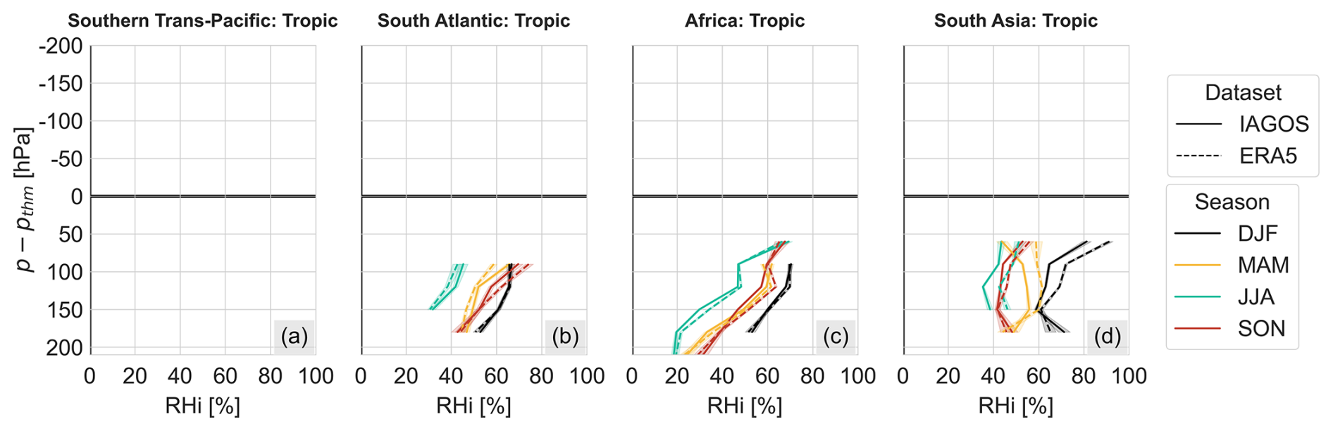
Figure A1 (a–d) Vertical distribution of IAGOS and ERA5 mean relative humidity over ice per season in the Southern Hemisphere tropical regions, with shading showing the 95 % confidence interval. Vertical levels are shown in terms of distance to the thermal tropopause (p−p_thm). We only consider vertical levels, seasons and regions with 500+ samples.

Appendix B: Distribution of temperature and relative humidity over ice with respect to thermal and dynamic tropopause

In this appendix, we present the vertical distribution of temperature and relative humidity over ice with respect to the thermal and dynamic tropopause. The tropopause data for both definitions are extracted from Hoffmann and Spang (2022). Since there can be two thermal tropopauses according to the World Meteorological Organization (WMO) definition (Hoffmann and Spang, 2022), we only consider the first WMO tropopause.

Figure B1 shows the vertical distribution of temperature and relative humidity over ice for the thermal and dynamic tropopause definitions from 1 July 2011 to 31 December 2022. We find similar distributions with both definitions, although there are some differences. For the vertical distribution of temperature, the dynamical and thermal tropopause show similar values for the mean and the 25 % and 75 % percentiles, especially in the upper troposphere. In the lower stratosphere, it is noticeable that the temperature gradient is sharper across the thermal tropopause in comparison to the dynamic tropopause. For the 99 % percentile, we notice that the thermal tropopause also has a sharper gradient in the upper troposphere, while for the 1 % percentile it is stronger for the dynamic tropopause. This is similar to observations by Petzold et al. (2020). Larger differences between the two tropopause definitions are noticeable for the vertical distribution of relative humidity over ice. In the lower stratosphere, larger values of RHi are found when using the dynamic tropopause definition, due to the larger 99 % percentile range, for which the thermal tropopause definition shows a sharper vertical gradient. This is also shown by the smaller mean RHi for the thermal tropopause compared to the dynamic tropopause. This may be the result of the thermal tropopause being located at a higher altitude than the dynamical tropopause (Petzold et al., 2020), for which drier conditions may be observed with this definition. This is also inline with reports by Petzold et al. (2020), who found a lower ISSR fraction in the lower stratosphere when using the thermal tropopause definition compared to the dynamic tropopause, indicating more moist conditions with the latter definition. We also find that the thermal tropopause is drier in comparison to the dynamic tropopause.

This analysis shows that the results are impacted by the choice of the tropopause definition. However, in this study, we are interested in the differences between IAGOS and ERA5, and are interested in the separation of dry and moist conditions. Although there are no significant differences in the results when using the thermal and dynamic tropopause definitions, there is a tendency for the dynamic tropopause definition to result in higher values of RHi in the lower stratosphere compared to the thermal tropopause definition. Therefore, we decided to use the thermal tropopause to ensure better separation of moist and dry conditions.

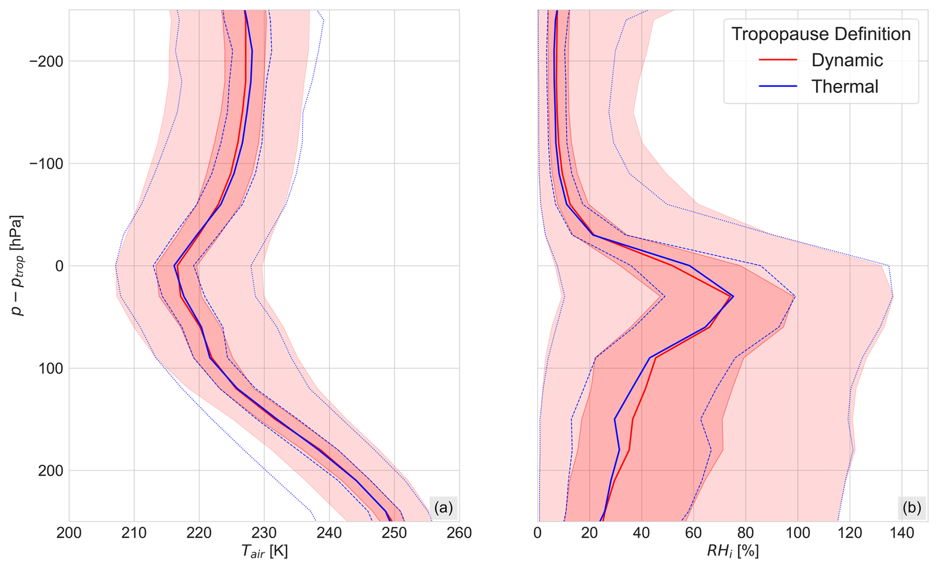
Figure B1 Vertical distribution of (a) temperature and (b) RHi for dynamic and thermal tropopause definitions using all considered IAGOS measurements in this study. Solid lines indicate mean values; dashed blue line and dark red shade indicate the 25 % and 75 % percentiles at the thermal and dynamical tropopause, respectively; similarly, dotted blue line and light red shade indicate the 1 % and 99 % percentiles.