Vegetation drag partition effects redistribute dust globally

Dust aerosols play a pivotal role in climate, ecosystems, and human health, yet global dust emission estimates in current Earth System Models (ESMs) remain highly uncertain due to over-simplified surface parameterizations and inconsistent particle size representations. Vegetation effects on dust emissions are often inconsistently and simplistically represented across models, limiting physical realism and land–atmosphere coupling. This study bridges this gap by utilizing the vegetation cover derived from the land surface model ORCHIDEE, and accounting for its effects on the dust emission scheme in the atmospheric model LMDzORINCA. The influence of including the very large dust particles (diameter greater than 100 µm) is also studied using two representations: a single-mode dominated by fine micrometre-sized particles, and a multi-mode representation comprising four size modes covering a range exceeding 100 µm. Incorporating vegetation reduces the global dust emissions by 23 %, primarily over semi-arid regions, and shifts the spatial dominance toward sparsely vegetated deserts, such as North Africa and East Asia. Including vegetation also leads to an improvement in model agreement with observations by reducing mean biases by approximately 50 %–80 % across various dust metrics, notably mitigating overestimations in dust aerosol optical depth (DAOD) over north-western India and in dust deposition over Antarctica. Furthermore, different particle size representations indicate that accurate reproduction of DAOD depends on the adequate representation of fine particles. Overall, this ESM-consistent framework, achieved by explicitly integrating vegetation effects and comprehensive particle size distributions, provides a pathway for future coupled land–atmosphere simulations under climate change.

1 Introduction

Mineral dust is a key component of the atmosphere, representing the largest source of primary aerosol emissions and contributing substantially to the global aerosol burden by mass (Checa-Garcia et al., 2021; Kok et al., 2023). Dust aerosols influence atmospheric stability, terrestrial and marine ecosystems, and human health through their emission, transport, and deposition (Tegen et al., 2002; Checa-Garcia et al., 2021). In source regions, dust emission is a direct manifestation of land surface erosion, leading to soil degradation, soil nutrient depletion, and vegetation deterioration (Shinoda et al., 2011; Wu et al., 2021). During atmospheric transport, suspended dust particles affect climate through interactions with other aerosols, scattering and absorption of solar and terrestrial radiation, modification of cloud properties, and by acting as a sink for radiatively important trace gases (Wu et al., 2021; Kok et al., 2023). The presence of dust particles in the near-surface atmosphere also degrades air quality, reduces visibility, and poses risks to human health (Achakulwisut et al., 2019; Wu et al., 2021). Upon deposition, mineral dust redistributes essential nutrients such as iron and phosphorus across terrestrial and marine ecosystems, and reduces snow surface albedo, thereby increasing solar absorption and accelerating melting, which ultimately shortens snow cover duration (Painter et al., 2007; Schulz et al., 2012).

Due to the significant role of dust in the Earth system (Mahowald, 2011; Kok et al., 2023), numerous studies have been dedicated to modelling the dust cycle, with the development of parameterizations and representations of dust emission (Marticorena and Bergametti, 1995; Ginoux et al., 2001; Tegen et al., 2002; Foroutan et al., 2017; Chappell et al., 2023), atmospheric loading (Tegen and Fung, 1995; Tanaka and Chiba, 2006; Schulz et al., 2012; Gui et al., 2022), climatic radiative effects (Miller et al., 2014; Balkanski et al., 2021; Adebiyi et al., 2023) and deposition (Zender et al., 2003; Lawrence and Neff, 2009; Schulz et al., 2012; Mahowald et al., 2017; Weis et al., 2024). Despite these efforts, significant discrepancies persist between model simulations and observational data, particularly for key metrics such as DAOD (Pu and Ginoux, 2018; Gkikas et al., 2022), total atmospheric dust loading (Ginoux et al., 2001; Zhao et al., 2022), and dust deposition (Anderson et al., 2016; Proestakis et al., 2025). A primary source of this divergence stems from the foundational stage of the dust cycle: dust emission. Current estimates of global annual dust emission exhibit substantial uncertainty, spanning a wide range from approximately 1000 to 9000 teragrams (Tg) per year, primarily due to inconsistent representations of the dust size distribution, associated microphysical properties, and surface conditions conducive to emissions (Kok et al., 2021a, b). Inaccuracies at this initial source stage inevitably propagate throughout all subsequent components of the model, compounding overall uncertainty (Leung et al., 2023; Chappell et al., 2023). Therefore, better constraining and accurately representing dust emission processes is fundamental to improving the fidelity of dust cycle simulations in models.

Dust originates mainly from bare soil, including deserts (Ginoux et al., 2001) and sparsely vegetated regions (Shinoda et al., 2011; Pierre et al., 2012). In semi-arid regions, surface vegetation emerges as a critical factor in regulating dust emission, through two main mechanisms (Pierre et al., 2012; Leung et al., 2023; AlNasser et al., 2025). First, vegetation attenuates wind erosivity by acting as a physical barrier that absorbs aerodynamic momentum from the wind, thereby reducing the shear stress on the erodible surface. Second, vegetation enhances soil resistance to wind erosion by increasing surface stability: the plant roots bind soil particles together, while the foliage shelters the ground and improves soil moisture retention. Specifically, by strengthening the cohesive forces between soil particles, vegetation significantly increases the threshold for wind erosion. Thus, accounting for vegetation effects is crucial to accurately representing the suppression of dust emissions.

Modelling the influence of vegetation on dust emission remains a critical challenge. Many traditional schemes treat the surface as aerodynamically bare, a simplified assumption that fails to capture the momentum absorption by roughness elements, thereby leading to potential overestimates of emissions in vegetated areas (Marticorena and Bergametti, 1995; King et al., 2005). Although tuning models against observed dust aerosol optical depth (DAOD) is a common strategy to mitigate such biases, it might obscure fundamental missing processes in the emission schemes and potentially induce artificial changes in dust emission (Chappell et al., 2023). This highlights the critical need for a more mechanistic representation of vegetation-induced surface roughness.

To date, only a limited number of process-oriented studies have explicitly investigated the effects of vegetation on dust emission as a primary focus. Nevertheless, such effects have already been incorporated in several Coupled Model Intercomparison Project (CMIP)-class models, such as UKESM (Woodward, 2001), CESM (Zender et al., 2003), and MPI (Stanelle et al., 2014), among others. Fundamentally, dust emission is initiated when the aerodynamic shear stress exerted by the wind exceeds a threshold friction velocity. To represent the suppressive effect of vegetation, models commonly apply drag partition schemes to reflect its attenuation on dust emission. Some models explicitly simulate the reduction of surface shear stress reaching erodible soils, typically as a function of vegetation-induced surface roughness length or roughness density (Shao et al., 1996; Okin, 2005; Foroutan et al., 2017; Klose et al., 2021). Other parameterizations represent this effect by enhancing the threshold friction velocity through a correction factor derived from vegetation-induced surface roughness (Okin, 2005; Foroutan et al., 2017; Wu et al., 2021).

While several models account for the suppression of dust emission by vegetation, various metrics of the presence of vegetation are used to represent their effects. Common proxies for vegetation include the fraction of absorbed photosynthetically active radiation, leaf area index (LAI), and albedo-based schemes designed to capture the sheltering effect of vegetation (Foroutan et al., 2017; Leung et al., 2023; Chappell et al., 2023). However, these indices are often empirical and rely on relatively simplified assumptions, for example, setting an upper LAI threshold of 0.3, above which dust emission is assumed to cease, often without sufficient testing or rigorous validation (Klose et al., 2021; Leung et al., 2023). Additionally, these proxies frequently rely on external satellite observations (e.g., MODIS) (Foroutan et al., 2017; Klose et al., 2021), rather than prognostic variables calculated within the Earth System Model, potentially leading to internal inconsistencies in land surface representation.

In summary, a major source of uncertainty in simulating global dust emission lies in how vegetation effects are represented in the existing models. Some advanced models utilize prescribed land-surface states to ensure realistic vegetation representation and computational efficiency, with the differences in the proxies and parameterizations used to represent vegetation effects, particularly regarding the partitioning of aerodynamic drag and the representation of surface roughness density, introducing methodological variability across different modelling frameworks (Shinoda et al., 2011; Klose et al., 2021). Despite this variability, the use of prescribed land-surface data represents a widely adopted and practical approach for investigating vegetation effects on dust emission. More complex configurations with interactive land–atmosphere coupling may further enable the investigation of feedback processes and facilitate future studies.

Beyond surface characteristics, the representation of dust particle size distribution (PSD) constitutes a primary source of uncertainty throughout the entire dust cycle. Historically, many global models prioritized fine-mode aerosols to limit computational cost and focus on their dominant role in aerosol-radiation interactions. However, recent observational evidence reveals that coarse and giant particles (e.g., diameter > 100 µm) account for a significant proportion of the atmospheric mass burden (Ryder et al., 2018; van der Does et al., 2018). The transition from the simplified fine-mode schemes to physically based, multi-modal distributions – though computationally intensive – is crucial for accurately simulating dust mass budget, extinction efficiency, transport, and deposition (Adebiyi and Kok, 2020; Di Biagio et al., 2020; Checa-Garcia et al., 2021). It further allows for a precise representation of PM₁₀ (particulate matter with aerodynamic diameter less than or equal to 10 µm), which is indispensable for air quality forecasting, as it directly impacts urban pollution levels and human respiratory health (Rodríguez et al., 2001; Querol et al., 2009). Consequently, evaluating model performance under different PSD configurations is essential to ensure the physical robustness of emission schemes and to investigate the size-dependent behaviour of dust aerosols in terms of loading, mass concentration, and deposition.

Prior to this study, LMDzORINCA, the atmospheric component of the Institut Pierre–Simon Laplace (IPSL) Earth System Model (ESM) (Boucher et al., 2020), did not account for the effects of vegetation on dust emissions, potentially leading to systematic overestimations of both emissions and the global atmospheric dust burden. In this study, the influence of vegetation on dust emissions is explicitly incorporated into the dust scheme in LMDzORINCA. We simulate vegetation cover by leveraging the recently upgraded dynamic grassland density representation within the model ORCHIDEE (ORganizing Carbon and Hydrology In Dynamic EcosystEms) (Xu et al., 2026), which is the land surface component of IPSL. This work thus represents the first assessment of how this new dynamic vegetation representation impacts global dust modelling within the IPSL framework. While the current integration is offline, it establishes a consistent framework for future fully coupled land–atmosphere simulations. Establishing such a coupled architecture is critical to resolving the non-linear feedbacks between dynamic ecosystems and the dust cycle, which is fundamental to understanding Earth system responses to rapid climate change.

To assess the impact of vegetation, we conduct a control simulation without the vegetation effects on dust emissions (default model configuration), and a vegetation-impact simulation, where the newly derived prescribed vegetation modulates the dust emission fluxes. Furthermore, the role of particle size representation is investigated by comparing a single-mode scheme (hereafter 1-mode) with a multi-mode scheme (hereafter 4-mode) to represent dust particle size distribution.

The remainder of this paper is organized as follows. Section 2 outlines the methodology, including the dust emission schemes, the derivation of fractional vegetation cover, the evaluation methods for dust aerosol optical depth (DAOD), dust surface concentration and deposition, and the model configurations. Section 3 provides a comparative analysis of the global and regional dust cycles – encompassing emissions, DAOD, surface particulate matter (PM) concentration, and total deposition – across the control and vegetation-impact simulations under both 1-mode and 4-mode configurations. Finally, Sect. 4 synthesizes the key findings in this study and outline future perspectives.

2 Methods

2.1 The dust emission schemes

This section details the framework adopted for modelling dust emission in this study. We first introduce the fundamental physical mechanism governing dust emission used in current models, followed by a description of the default emission scheme in the absence of vegetation, and then the revised emission scheme, which explicitly accounts for the vegetation effects.

2.1.1 Physical mechanism of dust emission

Dust emission is regarded as the aeolian transport of soil particles, primarily driven by saltation, which involves particles from 60 to 2000 µm (Marticorena and Bergametti, 1995; Foroutan et al., 2017). From a physical perspective, a particle at the surface is subject to gravitational force (F_G), cohesive forces (F_C) between particles, and the shear stress exerted by wind (Fig. 1a). The particle mobilization begins when the combined drag force (F_D) and lift force (F_L) – both resulting from the shear stress – collectively overcome the resisting forces of gravitational force (F_G) and cohesive forces (F_C), once the wind speed (u) surpasses a critical threshold known as threshold velocity (u_t). Particles lifted tens of centimetres above the surface eventually return as gravitational force (F_G) overcomes the lift force (F_L), generating horizontal flux in the form of saltation. During this process, soil aggregates undergo disaggregation both while airborne and upon surface impact. In the air, particles can fracture into smaller components; subsequently, the high-energy impact with the surface causes further fragmentation and breaks the cohesive bonds of the soil bed (sandblasting). These smaller particles can then be ejected vertically into the atmosphere, producing the vertical dust flux (Foroutan et al., 2017). The presence of vegetation on the surface modulates this process by increasing the u_t and reducing the exposed bare soil surface, thereby suppressing both horizontal and vertical emission fluxes (Fig. 1b).

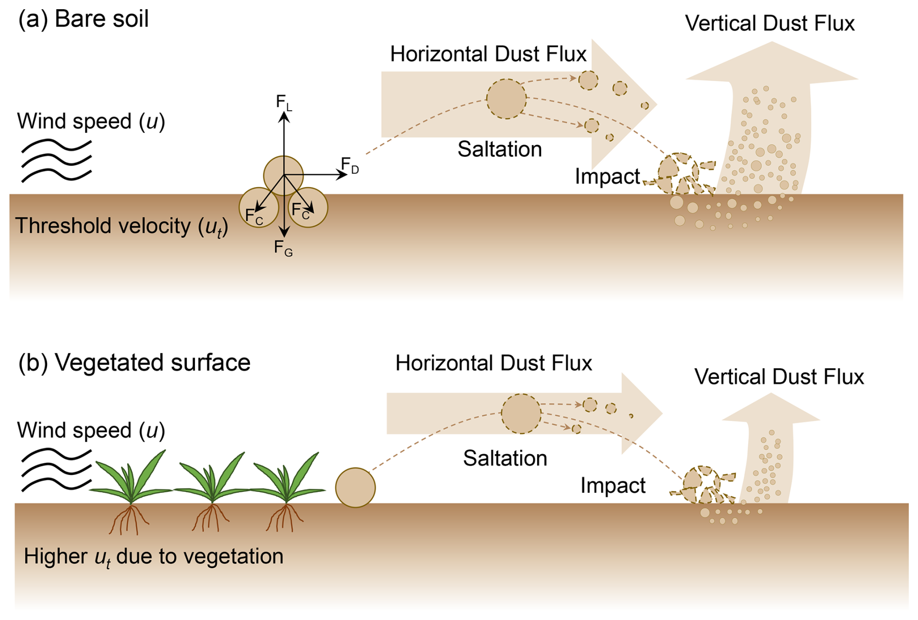
Figure 1 Conceptual diagram of aeolian dust emission processes on the (a) bare soil and (b) vegetated surfaces. The motion of air exerts a shear stress on the surface, driven by the near-surface wind speed (u). In panel (a), soil particles are subjected to four primary forces: the resisting forces of gravitational (F_G) and cohesive forces (F_C), as well as the initiating forces of aerodynamic drag (F_D) and lift (F_L), both derived from the wind. These forces determine the threshold velocity (u_t). The horizontal flux is dominated by the saltation of larger particles, while the vertical dust flux (suspension) into the atmosphere is primarily generated by the impact of these saltating particles, which triggers the ejection of smaller, non-saltating grains (Adapted from Foroutan et al., 2017). In panel (b), the presence of vegetation increases the u_t and thus suppresses both horizontal and vertical dust fluxes. The sizes of vegetation, particles, and flux arrows are schematic and not to scale.

The wind-induced horizontal flux (saltation) has been thoroughly characterized through extensive wind-tunnel experiments, with its magnitude empirically related to the wind velocity and the threshold velocity (Gillette, 1978; Goossens and Offer, 2000; Parajuli et al., 2016). However, the vertical dust flux (suspension) represents the final dust loading into the atmosphere. Due to the inherent difficulty in its direct observation, the vertical flux is typically parameterized as a function of the calculated horizontal flux (Marticorena and Bergametti, 1995). This vertical flux is the pivotal source term targeted by atmospheric modelling efforts, given its direct role in interacting with the radiation and climate system.

2.1.2 Default dust emission scheme

In the atmospheric model LMDzORINCA, dust mobilization is initiated if the following conditions are met:

1. Non-frozen or ice-free surface: Dust mobilization is restricted to surfaces not bound by ice or frost (Schulz et al., 2009). In this study, this is quantified by excluding regions where the mean January surface air temperature is below 0 °C, which mainly reflects Northern Hemisphere winter conditions and was originally optimized for major Northern Hemisphere sources;

2. Precipitation-limited source areas: The grid cell must be located within a predefined potential dust source area, where climatological annual precipitation is less than 300 mm (Schulz et al., 2009), representing regions with limited annual moisture supply as potential dust emitters;

3. Completely dry surface: Dust emission is restricted to a completely dry surface, quantified by a surface wetness proxy (water-equivalent depth, mm) that represents the moisture balance in the uppermost soil layer. Emission is permitted only when this proxy falls below a value of 10⁻¹⁰, which serves as a numerical threshold to enforce a dry surface condition and does not represent a physically meaningful soil moisture value.

Once all the prerequisites are satisfied, the dust emission flux (F_dust, unit: kg m⁻² s⁻¹) is calculated as below (Schulz et al., 2009):

$$\begin{array}{}\text{(1)}& F_{\mathrm{dust}}=\mathrm{MAX}\left[C\times u^{\mathrm{2}}\times \left(u-u_{\mathrm{t}}\right),\mathrm{0}\right]\end{array}$$

where C is the source strength factor (unit: kg s² m⁻⁵), u is the surface wind speed (unit: m s⁻¹), u_t is a threshold velocity (unit: m s⁻¹). The values of C, u, and u_t are calculated internally in other subroutines of the model.

Only when the wind speed (u) at the 30 min physical time step surpasses the threshold velocity (u_t) can the dust emission occur. In this scheme, u_t is derived by establishing a spatial correspondence between the region-specific threshold velocities calculated by Marticorena and Bergametti (1995) and the FAO soil types database within the Saharan Desert (Claquin et al., 1999; Schulz et al., 2009). Based on this correspondence, the model assigns a baseline u_t to each soil type according to the global FAO soil distribution, and adjusts the local u_t values to account for surface characteristics, such as topographic slopes and iron oxide content, which increase u_t due to aerodynamic sheltering and soil crusting, respectively. Consequently, the threshold velocity in this default scheme depends on soil types and geological properties, and does not include vegetation effects. This approach implies that whenever the emission conditions are met, the entire grid cell is treated as a homogeneous source, implicitly assuming a fully erodible surface and neglecting the suppressive effect of vegetation on bare soil exposure and particle mobilization. As a result, the default method tends to overestimate dust fluxes in areas with partial vegetation cover, and misrepresents the spatial heterogeneity of erodible surfaces.

2.1.3 Incorporating the effect of vegetation in dust emission scheme

To implement the vegetation's protective role into Eq. (1), we applied a correction factor to the threshold velocity (u_t), following the approach of Foroutan et al. (2017). Although a drag partitioning scheme, which computes the friction velocity (u_∗) to represent momentum transfer and shear stress at the air–surface interface, provides a more physically based representation of surface roughness (Kok et al., 2014; Klose et al., 2021), the emission scheme in LMDzORINCA is directly driven by the ambient wind speed (u) rather than u_∗. Under this formulation (Eq. 1), adjusting u_t provides a physically consistent way to account for vegetation by increasing the surface resistance to aeolian erosion.

The correction factor related to surface roughness (f_r) used to adjust the threshold velocity (u_t) was computed as follows (Foroutan et al., 2017):

$$\begin{array}{}\text{(2)}& \begin{array}{rl}{f}_{\mathrm{r}}& =\left[\left(\mathrm{1}-{\mathit{\sigma }}_{\mathrm{v}}{m}_{\mathrm{v}}{\mathit{\lambda }}_{\mathrm{v}}\right)\left(\mathrm{1}+{\mathit{\beta }}_{\mathrm{v}}{m}_{\mathrm{v}}{\mathit{\lambda }}_{\mathrm{v}}\right)\right.\\ & {\left.\left(\mathrm{1}-{\mathit{\sigma }}_{\mathrm{s}}{m}_{\mathrm{s}}{\displaystyle \frac{{\mathit{\lambda }}_{\mathrm{s}}}{\mathrm{1}-A_{\mathrm{v}}}}\right)\left(\mathrm{1}+{\mathit{\beta }}_{\mathrm{s}}{m}_{\mathrm{s}}{\displaystyle \frac{{\mathit{\lambda }}_{\mathrm{s}}}{\mathrm{1}-A_{\mathrm{v}}}}\right)\right]}^{\mathrm{0.5}}\end{array}\end{array}$$

where σ_v, m_v, β_v, σ_s, m_s, and β_s are coefficients with values adopted from previous literature (Darmenova et al., 2009; Xi and Sokolik, 2015). The variable λ_s represents the density of non-vegetation roughness solid elements, such as rocks and pebbles, with values ranging from 0.002 to 0.2 (Marticorena et al., 2006; Foroutan et al., 2017). In this study, the lower bound of the reported range 0.002 was adopted to represent conditions with minimal non-vegetative solid obstacles, in order to minimize background interference, allowing us to focus on the role of vegetation in drag partitioning. The variable λ_v represents the roughness density of vegetation, which is calculated as a function of the fraction of vegetation cover (A_v) (Foroutan et al., 2017):

$$\begin{array}{}\text{(3)}& {\mathit{\lambda }}_{\mathrm{v}}=-\mathrm{0.35}\ln \left(\mathrm{1}-A_{\mathrm{v}}\right)\end{array}$$

The value of A_v was derived from the land surface model ORCHIDEE, which will be introduced in the following section. The positive correlation between A_v and f_r (Fig. S1 in the Supplement) shows that the correction factor (f_r) increases with vegetation cover (A_v), exhibiting a sharp non-linear increase especially when A_v exceeds 0.9.

Based on the correction factor (f_r), we thus used a new equation for dust emission to incorporate vegetation effects as follows:

$$\begin{array}{}\text{(4)}& \begin{array}{rl}{F}_{\mathrm{dust}}& =\left(\mathrm{1}-A_{\mathrm{v}}\right)\times \mathrm{MAX}\left[C\times u^{\mathrm{2}}\times \left(u-u_{\mathrm{t}}\right),\mathrm{0}\right]\\ & +A_{\mathrm{v}}\times \mathrm{MAX}\left[C\times u^{\mathrm{2}}\times \left(u-f_{\mathrm{r}}\times u_{\mathrm{t}}\right),\mathrm{0}\right]\end{array}\end{array}$$

This formulation can be interpreted as a first-order approximation between two limiting cases: (i) a segregated case, implying a complete spatial separation between vegetation and bare soil, thereby no vegetation-induced shielding of bare soil emissions, as expressed by the first term in Eq. (4); and (ii) an interspersed case, where the uniform distribution of vegetation reflects the effective protection from vegetation, as expressed by the second term in Eq. (4). Accordingly, total dust emissions at the grid scale are computed as an area-weighted combination of these two limiting cases, thereby representing intermediate conditions and capturing sub-grid surface heterogeneity without explicitly resolving their spatial organization of vegetation patterns (Deblauwe et al., 2008).

Emissions from the first term of Eq. (4) that represents the contribution from surfaces without vegetation protection, occurs only when the default threshold velocity (u_t) is exceeded. Conversely, emissions from the second term accounting for the vegetation effect, are determined by a modified threshold velocity (u_t×f_r), where the correction factor (f_r≥1) represents the additional aerodynamic resistance induced by vegetation elements. Therefore, unlike the default scheme (Sect. 2.1.2), this revised approach (Eq. 4) suppresses dust emission by increasing the threshold velocity for the vegetated fraction, providing a more physically consistent representation of sub-grid emission processes.

Within potential source regions, the land surface is assumed to be composed of bare soil and vegetation. Anthropogenic land types, such as urban areas and irrigation-related water bodies, are excluded to maintain the focus on natural mineral dust emissions (Ginoux et al., 2012). Furthermore, surfaces covered by permanent ice, snow, or water are treated as non-emissive, consistent with the conditions for dust emission in the model (Sect. 2.1.2).

To evaluate the threshold velocity used in this study, we compared it with the observationally retrieved 10 m wind speed threshold (V_threshold) from Pu et al. (2020), which identifies active dust emission events using region-specific dust aerosol optical depth (DAOD) criteria (0.5 for arid regions and 0.05 for semi-arid regions; Fig. S2a–c). Overall, u_t aligns with V_threshold in major desert regions but is higher in vegetated secondary sources (Fig. S2d–e). We provide the more detailed comparison and analysis in Sect. S1 (Supplement).

2.2 Fraction of vegetation cover (A_v) derived from ORCHIDEE

The global process-based model ORCHIDEE is capable of simulating the coupled carbon, nitrogen, water, and energy cycles, including vegetation dynamics, biogeochemical fluxes, and plant competition (Krinner et al., 2005; Naudts et al., 2015; Vuichard et al., 2019). In ORCHIDEE, each grid cell contains up to 15 plant functional types (PFTs), representing eight different types of forests, four types of grasslands, two types of croplands, and bare soil (defined as a separate PFT). The sum of the fraction of each PFT (V_fra) is unity for each grid cell.

To address the limitations of the fixed grassland density in ORCHIDEE's default configuration, which restricts the representation of bare soil within grasslands, a dynamic density approach (revision 9010 in the ORCHIDEE Subversion (SVN) trunk) has been developed for grasslands. This updated approach has been shown to improve the spatial representation of fractional vegetation cover when evaluated against the Copernicus Land Monitoring Service FCOVER dataset (Copernicus Land Monitoring Service, 2020), compared to the default fixed density approach (Xu et al., 2026), with correlation coefficient increasing from 0.11 to 0.26. In this study, we leveraged the fractional vegetation cover (A_v) derived from this dynamic grassland density approach.

Given that the vegetated regions associated with dust emission are primarily linked to grasslands (Shinoda et al., 2011), this study focuses on three key PFTs characteristic of (semi-)arid environments: temperate C₃ grassland, tropical C₃ grassland, and C₄ grassland. Boreal grasslands were excluded, and forests and croplands were assumed to have a negligible erodible bare soil fraction. This simplification allows us to focus on capturing the dominant dust-emitting regions within (semi-)arid environments, while acknowledging that boreal grasslands, sparse forests, and croplands may contain bare soil patches capable of contributing to dust emissions.

In this way, we can derive the fraction of bare soil (F_bare) in one grid cell composed of pure bare soil (treated as a separate PFT), as well as the fraction of bare soil gaps in the grasslands, as:

$$\begin{array}{}\text{(5)}& \begin{array}{rl}{F}_{\mathrm{bare}}& =V_{\mathrm{fra},\mathrm{bare}}+V_{\mathrm{fra},\mathrm{temp}{\mathrm{C}}_{\mathrm{3}}}\times \left(\mathrm{1}-D_{\mathrm{temp}{\mathrm{C}}_{\mathrm{3}}}\right)\\ & +V_{\mathrm{fra},\mathrm{C}\mathrm{4}}\times \left(\mathrm{1}-D_{{\mathrm{C}}_{\mathrm{4}}}\right)+V_{\mathrm{fra},\mathrm{trop}{\mathrm{C}}_{\mathrm{3}}}\times \left(\mathrm{1}-D_{\mathrm{trop}{\mathrm{C}}_{\mathrm{3}}}\right)\end{array}\end{array}$$

where V_fra,bare, $V_{\mathrm{fra},\mathrm{temp}{\mathrm{C}}_{\mathrm{3}}}$, $V_{\mathrm{fra},{\mathrm{C}}_{\mathrm{4}}}$, and $V_{\mathrm{fra},\mathrm{trop}{\mathrm{C}}_{\mathrm{3}}}$ refer to the fraction of vegetation type of pure bare soil, temperate C₃ grassland, C₄ grassland, and tropical C₃ grassland in one grid cell, respectively; $D_{\mathrm{temp}{\mathrm{C}}_{\mathrm{3}}}$, $D_{{\mathrm{C}}_{\mathrm{4}}}$, and $D_{\mathrm{trop}{\mathrm{C}}_{\mathrm{3}}}$ represent the grassland density of temperate C₃ grassland, C₄ grassland, and tropical C₃ grassland, respectively. In the ORCHIDEE model, grassland density (D) is defined as the fractional area occupied by “conceptual individuals” – each assumed to cover 1 m² – within the grassland PFT's area (Xu et al., 2026). Consequently, D is a dimensionless quantity (m² m⁻²), ranging from 0.05 (a minimum threshold for numerical stability) to 1.0 (full coverage). The grassland density (D) is dynamically simulated by ORCHIDEE, varying based on indicators such as reserve and labile carbon, reflecting vegetation response to resource availability. The monthly output of simulated D serves as a time-varying input for the F_bare calculation in Eq. (5).

The fraction of bare soil gaps within the grassland PFT is expressed as (1−D), representing the portion of the grassland area not covered by vegetation. This is shown for each grassland (Fig. S3a–c) and their sum (Fig. S3d), and is compared to the fraction of pure bare soil (Fig. S3e). While pure bare soil dominates in hyper-arid regions such as North Africa, the bare soil gaps within grasslands become more prominent in (semi-)arid regions including the western USA, southern Africa, and India, where they can locally exceed the contribution of pure bare soil (Fig. S3f).

The vegetation cover fraction (A_v) can be calculated as the complement of the fraction of bare soil:

$$\begin{array}{}\text{(6)}& A_{\mathrm{v}}=\mathrm{1}-F_{\mathrm{bare}}\end{array}$$

In ORCHIDEE, building on the equilibrium with a 200-year spin-up, a continuous transient simulation was performed for 2004–2020 using interannual meteorological forcing, ensuring that the land surface state – including that of 2008 – evolves consistently with climate variability. A static land-use map, based on the ESA CCI Land Cover map (ESA, 2017), was maintained throughout the period to isolate the influence of land cover change (Xu et al., 2026). The output of grassland density was simulated at the standard 2°×2° spatial resolution. The data of A_v (Fig. S4a) and f_r (Fig. S4b) derived from ORCHIDEE were regridded in Python using the griddata function from SciPy with nearest-neighbor interpolation to the spatial resolution (2.5° longitude × 1.27° latitude) in LMDzORINCA.

2.3 Model description, dust cycle representation, and evaluation framework

This section first outlines the general description and configuration of the LMDzORINCA model, then details the treatments for the simulated dust cycle, including dust aerosol optical depth (DAOD), surface PM concentrations, and deposition. These simulated fields are evaluated against the direct site-based observations and state-of-the-art observationally constrained benchmarks, with the summary of the statistical metrics and treatments at the end of this section.

2.3.1 Model Description

The global chemistry-aerosol-climate model LMDzORINCA consists of the general circulation model LMDz (Laboratoire de Météorologie Dynamique, z refers to model's zoom capacity; Hourdin et al., 2013), coupled to the chemistry and aerosol model INCA (INteraction with Chemistry and Aerosols), and the land surface model (LSM) ORCHIDEE (ORganizing Carbon and Hydrology In Dynamic EcosystEms). This integrated framework simulates the exchanges between the atmosphere and the terrestrial ecosystem (Hauglustaine et al., 2014) and forms a core component of the IPSL Earth System Model (Boucher et al., 2020).

The model solves the primitive equations using a finite-difference formulation (Hauglustaine et al., 2004) with a 3-minute time step. Atmospheric transport is computed with a finite-volume second-order scheme, applied every 15 min for large-scale advection (Hauglustaine et al., 2004). The deep convection and turbulent mixing parameterizations follow the “New Physics” scheme (Boucher et al., 2020), using a 30 min time step for physical processes.

In LMDzORINCA, dust is treated as an insoluble natural mineral aerosol, excluding any anthropogenic contributions. Following the microphysical constraints established by Di Biagio et al. (2020), the dust particle size distribution (PSD) contains four lognormal modes. Each mode is characterized by a specific mass median diameter (MMD) and a constant geometric standard deviation (σ): (1) Mode 1: MMD = 1 µm and σ= 1.8; (2) Mode 2: MMD = 2.5 µm and σ=2.0; (3) Mode 3: MMD = 7 µm and σ=1.9; and (4) Mode 4: MMD = 22 µm and σ=2.0. Depending on the simulation requirements, these modes can be utilized either individually or collectively as a superposition.

The model's horizontal resolution consists of 144×143 grid points (2.5° in longitude and 1.27° in latitude), with time steps of 30 min for the chemistry and 2 min for the physics. The vertical column is divided into 79 layers, extending from the surface to about 80 km in altitude.

2.3.2 Simulation configurations

To investigate how vegetation influences the dust cycle, we conducted two simulations for the year 2008 under the LMDzORINCA modelling framework, including the control simulation (Sect. 2.1.2) and the vegetation-impact simulation (Sect. 2.1.3). In both simulations, climate and aerosols were decoupled in the model. This decoupled configuration allows us to isolate the impact of vegetation on dust emissions – which is the focus of this study – by eliminating feedbacks from meteorological variables such as precipitation and temperature that would otherwise arise from aerosol–climate interactions.

To evaluate the effect of dust particle size distribution (PSD), both control and vegetation-impact simulations were performed using two representations of the PSD. The 1-mode configuration was represented exclusively by Mode 2 (MMD = 2.5 µm), whereas the 4-mode configuration utilized a more complete description of the PSD that consists of four modes as described in Di Biagio et al. (2020) – with MMDs of 1, 2.5, 7, and 22 µm.

In dust modelling, although the physical understanding of the mechanisms governing dust emission is well established, detailed information on the fine-scale surface features that determine the local conditions is largely missing, hindering the accurate parameterization of emission thresholds. To better represent the spatial distribution and magnitude of global dust emissions, global modelers generally use observational constraints to rescale the emissions over large desert regions (Adebiyi et al., 2020; Kok et al., 2021b; Li et al., 2022; Leung et al., 2023).

In this study, we used the observational constraint – Dust Constraints from joint Experimental–Modeling–Observational Analysis (DustCOMM) by Kok et al. (2021b) – to calibrate our emission scheme. First, target regional emissions (locations shown in Fig. S5) were derived by applying the relative regional contributions from DustCOMM to the global total emission obtained in the 1-mode vegetation-impact simulation. Second, regional rescaling factors were calculated as the ratio between these target emissions and the original output of dust emission in these regions (Table S1 in the Supplement). These factors were then applied to all grid cells within the designated source regions (Fig. S5), while a factor of unity (1.0) was assigned to areas outside these regions. The same set of rescaling factors (Table S1) was applied to all simulations to ensure that any divergence between the control and vegetation-impact simulations was strictly attributable to the explicitly parameterized inhibitory effects of vegetation, rather than being masked or distorted by differential model tuning. These rescaling factors can be used to account for biases in regional dust emissions and to provide an observational constraint. A discussion of the potential sources of regional biases is provided in Sect. 3.5.

In this study, the model was run in a nudged mode for the year 2008, in which the winds were relaxed toward ECMWF (European Centre for Medium-Range Weather Forecasts) reanalysis data through a correction term with a 2.5 h relaxation time (Hauglustaine et al., 2004) to constrain the atmospheric state (Schulz et al., 2009). Model outputs for aerosols and gases, which were computed every 30 min, were archived at a monthly temporal resolution. These outputs include dust emission, dust load, mass mixing ratio, and three deposition fluxes which represent separate physical processes: wet deposition, dry deposition, and sedimentation.

2.3.3 Dust aerosol optical depth (DAOD)

As a critical metric of the global dust cycle, dust aerosol optical depth (DAOD) quantifies the extinction of solar radiation by particles at a given wavelength, thereby affecting the terrestrial radiation balance and subsequent climate feedbacks (Pu and Ginoux, 2018). The simulated DAOD at 550 nm was calculated a posteriori based on monthly model outputs using the following equation:

$$\begin{array}{}\text{(7)}& \mathrm{DAOD}=\mathrm{1000}\times \mathit{\theta }\times L\end{array}$$

where θ refers to the mass extinction efficiency (MEE), with values of 1.96, 0.82, 0.22 and 0.069 m² g⁻¹ assigned to Modes 1 to 4, respectively (Sect. 2.3.1), and L refers to dust load in the unit kg m⁻², with values simulated by the LMDzORINCA model.

To evaluate the simulated DAOD, two types of observational benchmarks were utilized: (1) Site-based mean annual observations, providing localized measurements; (2) Observationally constrained regional and seasonal datasets, offering a broader spatial and temporal perspective on model performance.

The site-based observational data for DAOD at 550 nm were derived from the Aerosol Robotic NETwork Spectral Deconvolution Algorithm (AERONET-SDA) product for the year 2008. We utilized AERONET Version 3.0 and the SDA Version 4.1 products (AERONET, 2025). Site selection (including 18 sites shown in Fig. 2a) focused on dust-dominated regions (Albani et al., 2014; Kok et al., 2014; Leung et al., 2024), with any site lacking data for 2008 being excluded from this analysis. For these sites, data retrieval levels prioritized level 2.0, substituting with level 1.5 only when level 2.0 data was unavailable (Leung et al., 2024). The initial AERONET retrievals were aggregated into monthly averages, and the mean annual DAOD for each site was calculated by averaging only the valid monthly records. The coarse-mode aerosol fraction from the SDA product was explicitly selected as the representative proxy for dust aerosol (Leung et al., 2024). These selected sites were then systematically classified into 15 distinct regions (Fig. S6) based on the geographic boundaries defined by Kok et al. (2021a). Observational sites located marginally outside these boundaries were assigned to the nearest region based on their geographical location.

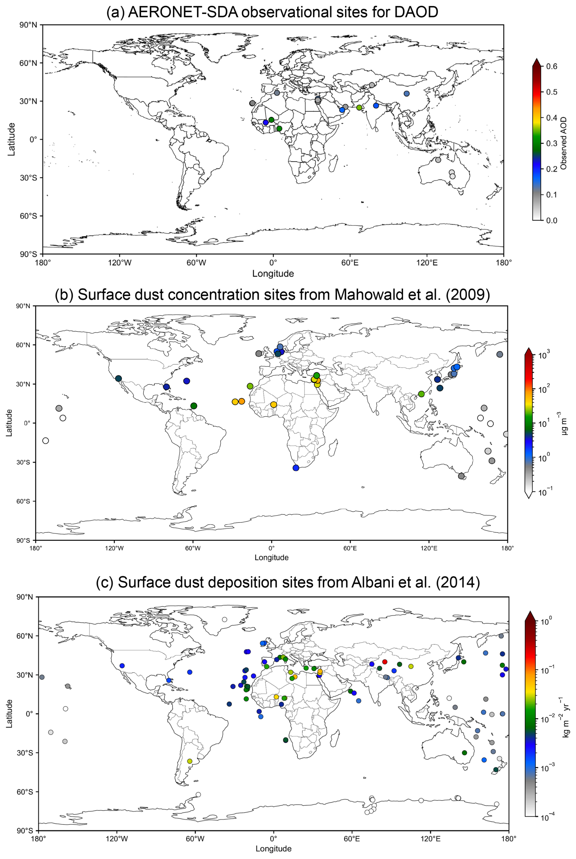
Figure 2 Spatial distribution of the observational sites used for model evaluation: (a) DAOD from AERONET-SDA, (b) surface dust concentration (µg m⁻³), and (c) surface dust total deposition (kg m⁻² yr⁻¹).

To ensure a robust evaluation, the regional and seasonal DAOD values, constrained based on observations and model ensembles (Table 2 in Kok et al., 2021a), serve as an additional basis for comparison with our simulated DAOD results. The data were averaged over 15 regions (Fig. S6) during the four standard meteorological seasons: DJF (December, January, and February), MAM (March, April, and May), JJA (June, July, and August), and SON (September, October, and November), for the years spanning from 2004 to 2008.

To facilitate the model-to-observation comparison, spatial alignment between the coarse-resolution model grid cells and observational coordinates was achieved using a bilinear interpolation approach. This scheme, implemented via the RegularGridInterpolator from the Python SciPy library, enabled model outputs to be mapped to the exact geographical coordinates of each monitoring station. In addition, the simulated mean annual DAOD at global and regional scales was calculated by averaging 12 monthly outputs, and to account for the spherical geometry of the Earth, an area-weighted averaging method was applied based on the specific area of each grid cell.

To ensure that the simulated global mean annual DAOD aligns with the benchmark range of 0.030 ± 0.005 established by Ridley et al. (2016), we introduced global scaling coefficients, a for the 1-mode configuration, and b specifically for Mode 2 and Mode 3, while Mode 1 and Mode 4 were left unchanged in the 4-mode configuration. This strategy is based on the fact that Mode 2 and Mode 3 contribute most significantly to the global DAOD (together accounting for ∼ 80 %), whereas Mode 1 and Mode 4 have a smaller contribution (Di Biagio et al., 2020). To ensure consistency throughout the dust cycle, these global scaling coefficients were systematically applied offline to the monthly model output (including dust emission, DAOD, surface PM concentration, and deposition) as part of an a posteriori calibration. Although applying such scaling coefficients to emission slightly modifies the relative mass contributions of different size modes within the 4-mode configuration, the intrinsic microphysical properties of each mode (e.g., MMD and σ) remain consistent with the original parameterization.

The calibration process prioritized maintaining the global mean annual DAOD within the target range of 0.030 ± 0.005, while simultaneously optimizing the model's overall statistical performance against independent observational datasets for DAOD, surface PM, and total deposition. Sensitivity analysis (Table S2) revealed that the optimal scaling coefficients are 0.74 for a, and 1.24 for b. Other coefficients produced a higher global mean annual DAOD and resulted in weaker correlation with observations in the 4-mode configuration (Table S2). To isolate the suppressive effects of vegetation, the same set of global scaling coefficients was consistently applied to both the control and vegetation-impact simulations within each size-mode configuration.

2.3.4 Dust surface particulate matter (PM) concentration

Surface dust PM concentrations are determined by the combined effects of vegetation-modulated emissions and subsequent atmospheric transport and deposition processes. These highly nonlinear and interconnected processes are sensitive to surface roughness, meteorological conditions (e.g., wind speed, precipitation, and large-scale circulation), boundary-layer dynamics (e.g., planetary boundary layer height), deposition parameterizations, and particle size distributions (Shao, 2008; Ginoux et al., 2001).

Surface-level dust PM concentration represents the mass of dust particles suspended per unit volume of air within the lowest atmospheric layer, typically expressed in the unit of µg m⁻³. The simulated dust PM concentration (C_dust, µg m⁻³) for each grid cell is derived based on the dust mass mixing ratio (R_dust) and the air density (D_air, µg m⁻³) as:

$$\begin{array}{}\text{(8)}& C_{\mathrm{dust}}=R_{\mathrm{dust}}\times D_{\mathrm{air}}\end{array}$$

where both R_dust and D_air are simulated by the model.

In situ observations for dust PM concentration were determined through the compilation of previous studies presented in supplemental Table 2 by Mahowald et al. (2009). The specific sites selected for comparison in this study were chosen according to Leung et al. (2024) and Li et al. (2022) with 42 locations shown in Fig. 2b. Since the original observational data reported iron concentration, the equivalent dust concentration was estimated based on the specific iron content in dust, which is approximately 3.5 % (Mahowald et al., 2009).

To enable a point-to-point comparison, simulated concentrations were interpolated to the geographical coordinates of the observational sites using bilinear interpolation. In the 4-mode configuration, in order to align with the aerodynamic sampling cut-off of PM₁₀ monitoring instruments, the simulated PM₁₀ concentrations were calculated by applying the mode-specific mass fractions ($F_{{\mathrm{PM}}_{\mathrm{10}}}$) to each of the four modes. Based on the Particle Size Distribution (PSD) described in Sect. 2.3.1, the $F_{{\mathrm{PM}}_{\mathrm{10}}}$ values for Modes 1 through 4 are: 1.00, 0.98, 0.71, and 0.13, respectively.

2.3.5 Dust surface total deposition

The dust surface total deposition (in the unit of kg m⁻² yr⁻¹) is computed as the sum of three removal processes: sedimentation, wet and dry deposition.

Wet deposition represents the removal of particles from the atmosphere through their incorporation into cloud droplets (in-cloud scavenging) or their removal by falling hydrometeors below the cloud base (below-cloud scavenging). The total wet deposition flux consists of two distinct mechanisms: convective scavenging following the schemes of Liu et al. (2001) and large-scale stratiform scavenging following the schemes of Giorgi and Chameides (1986) and Balkanski et al. (1993). The model sequentially updates the dust mass mixing ratio to reflect the removal during convective transport as well as both convective and stratiform precipitation.

The dry deposition process is parameterized as a downward mass flux at the surface interface, representing the non-gravitational removal of particles onto land and ocean surfaces via turbulent diffusion, impaction, and interception. The dry deposition flux is calculated as the product of the dust mass concentration in the surface layer and its corresponding dry deposition velocity, which accounts for aerodynamic, quasi-laminar boundary layer and surface resistances (Hauglustaine et al., 2004).

Sedimentation refers to the gravitational settling of particles, governed by their terminal velocities determined by applying the Cunningham slip correction to the Standard Stokes velocity. To account for the settling of size-distributed dust modes, the model incorporates a Slinn correction factor (Slinn and Slinn, 1980) as a function of the mass median diameter (MMD) and the geometric standard deviation (σ), as implemented in the LMDzORINCA framework (Hauglustaine et al., 2004).

The observational dataset for dust total deposition was obtained from the compilation originally presented in Table S2 of Albani et al. (2014). To derive surface PM₁₀ deposition from the observational dataset, the observed total dust deposition values were multiplied by the fraction of PM₁₀ provided by Albani et al. (2014). Two European high-altitude sites, Colle del Lys and Colle Gnifetti, were excluded from the dataset because their elevations are much higher than the mean surface elevation of the corresponding grid cells in the model orography. The model's elevation of 1336 m fails to resolve the complex orography at the specific coordinates (Colle del Lys: 45.06° N, 7.35° E, actual 1779 m; Colle Gnifetti: 46° N, 7° E, actual 4452 m; elevations retrieved from Mapy.cz, 2025). The locations and observed values for the 105 observational sites are shown in Fig. 2c.

To facilitate the comparison with station-based observations, simulated deposition fluxes were extracted at the exact coordinates of each site using bilinear interpolation on the model's regular latitude-longitude grid. In the 4-mode configuration, the $F_{{\mathrm{PM}}_{\mathrm{10}}}$ values (Sect. 2.3.4) were applied to the simulated deposition flux in each mode.

To evaluate the model's performance across different deposition environments, we distinguished between observations from terrestrial and oceanic stations, where the corresponding grid cells were identified using a global land mask (NASA GPM, 2025). Since the thresholds that define a sea surface are often chosen to range from 100 % (strictly open water) down to 75 % (including seaward coastal areas), in this study we conservatively regarded grid cell values greater than or equal to 75 % as the oceanic grid cells, treating the remainder as terrestrial grid cells. Furthermore, deposition sites located within the Pacific and Atlantic basins were treated as representative of oceanic environments, regardless of the specific mask values. This ensures that remote island stations were included in the ocean deposition analysis, as their observations primarily reflect open-ocean conditions rather than large-scale continents.

2.3.6 Statistical metrics

Five key statistical metrics were chosen in this study to evaluate the agreement between simulated values and observational datasets: The coefficient of determination (R²), the Pearson correlation coefficient (R), root mean square error (RMSE), normalized RMSE (NRMSE), and mean bias (MB). The formulas used to compute these metrics are listed below. In all equations, y_i refers to the ith observational data value, ${\widehat{y}}_i$ refers to the ith simulated data value, and N is the total number of samples.

R² represents the proportion of the variance in the observational data that is predictable from the model, calculated as:

$$\begin{array}{}\text{(9)}& R^{\mathrm{2}}=\mathrm{1}-{\displaystyle \frac{\sum _{i=\mathrm{1}}^N{\left({\widehat{y}}_i-y_i\right)}^{\mathrm{2}}}{\sum _{i=\mathrm{1}}^N{\left(\overline{y}-y_i\right)}^{\mathrm{2}}}}\end{array}$$

where the $\overline{y}$ refers to the mean of the all observed values.

R measures the strength and direction of the linear relationship between the simulated results and the observations, calculated as:

$$\begin{array}{}\text{(10)}& R={\displaystyle \frac{\sum _{i=\mathrm{1}}^N\left(y_i-\overline{y}\right)\left({\widehat{y}}_i-\overline{\widehat{y}}\right)}{\sqrt{\sum _{i=\mathrm{1}}^{\mathrm{N}}{\left(y_i-\overline{y}\right)}^{\mathrm{2}}}\sqrt{\sum _{i=\mathrm{1}}^N{\left({\widehat{y}}_i-\overline{\widehat{y}}\right)}^{\mathrm{2}}}}}\end{array}$$

where the $\overline{\widehat{y}}$ refers to the mean of the all simulated values.

The RMSE quantifies the average magnitude of the error, calculated in the following equation:

$$\begin{array}{}\text{(11)}& \mathrm{RMSE}=\sqrt{{\displaystyle \frac{\sum _{\mathrm{i}=\mathrm{1}}^N{\left({\widehat{y}}_i-y_i\right)}^{\mathrm{2}}}{N}}}\end{array}$$

The NRMSE provides a dimensionless measure of the error by normalizing the RMSE to the mean of the observational data, calculated as:

$$\begin{array}{}\text{(12)}& \mathrm{NRMSE}={\displaystyle \frac{\mathrm{RMSE}}{\overline{y}}}\end{array}$$

For variables evaluated in logarithmic space (log₁₀), the NRMSE_log was calculated by normalizing the RMSE_log with respect to the range of the observed log-values (log₁₀(y_max)−log₁₀(y_min)). This approach ensures a positive and stable denominator, as the mean of log-transformed values (e.g., for deposition < 1 kg m⁻² yr⁻¹) can be negative or near-zero.

$$\begin{array}{}\text{(13)}& {\mathrm{NRMSE}}_{\log }={\displaystyle \frac{{\mathrm{RMSE}}_{\log }}{{\log }_{\mathrm{10}}\left(y_{\max }\right)-{\log }_{\mathrm{10}}\left(y_{\min }\right)}}\end{array}$$

Finally, the MB indicates the average systematic error of the simulation, revealing whether the model generally overestimates (MB > 0) or underestimates (MB < 0) the observed values, which is formulated as:

$$\begin{array}{}\text{(14)}& \mathrm{MB}={\displaystyle \frac{\sum _{i=\mathrm{1}}^N\left({\widehat{y}}_i-y_i\right)}{N}}\end{array}$$

To ensure the robustness and accuracy of the model evaluation metrics, different data processing approaches were applied based on the characteristics of the variables. For dust emission and DAOD, the statistical metrics were calculated directly using the original values, as their magnitudes are relatively consistent. By contrast, for variables including dust surface PM concentration and deposition, the data often spans several orders of magnitude. Therefore, all statistical metrics for these variables were calculated in the logarithmic space (log₁₀). This transformation helps normalize the distribution and ensures that model performance is equally weighted across the entire range of data magnitudes (Leung et al., 2024). The resulting statistical metrics are summarized in Table S3.

2.3.7 Summary of treatments in the study

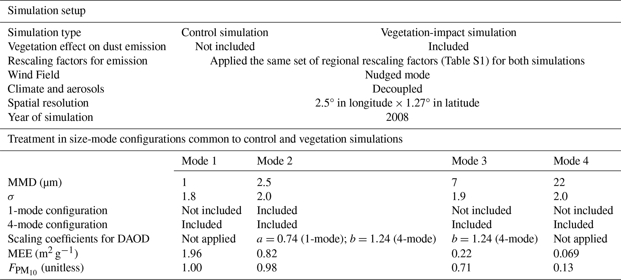
To provide a comprehensive overview of the simulation framework, Table 1 summarizes the key configurations for the simulations and experimental setups, such as the rescaling factors used to match the regional dust emission fluxes from DustCOMM (Kok et al., 2021b), wind field and climate-aerosol decoupling. It also contains the size-mode specifications, including the mass median diameters (MMD), geometric standard deviations (σ), global scaling coefficients (a and b) to match observationally constrained DAOD benchmark of Ridley et al. (2016), as well as the mass extinction efficiencies (MEE), and PM₁₀ mass fractions ($F_{{\mathrm{PM}}_{\mathrm{10}}}$) associated with each particle size mode.

Table 1 Summary of experimental design and model configurations in this study.

3 Results and discussions

In this section, we analyse the impact of vegetation and the representation of dust particle size on the global dust cycle in terms of four key indicators. Specifically: emission, DAOD, surface PM concentration, and deposition.

For the 4-mode configuration, the global maps for dust emission and DAOD illustrate the aggregate sum of all four modes to provide a more comprehensive view. For the dust surface PM concentration and deposition, the $F_{{\mathrm{PM}}_{\mathrm{10}}}$ (Table 1) is applied to each individual mode to represent the PM₁₀ component in the 4-mode configuration. In contrast, in the 1-mode configuration, all the results for global spatial maps and comparisons with observation are derived from the simulated data of Mode 2, which represents the single focus of this setup. For clarity, this section mainly focuses on results from the vegetation-impact simulation in the 4-mode configuration, while results from the control simulations and the 1-mode configuration are presented in the Supplement.

3.1 Impact of vegetation on global dust emission

Simulated dust emissions (Figs. 3a, S7a) in 4-mode configuration were primarily concentrated in the Sahara Desert (North Africa), the Kyzylkum Desert (central Asia), and the Turkestan and Gobi Deserts (East Asia), compared with a relatively modest amount of dust emissions in North America, southern Africa, and Australia. The 1-mode configuration (Fig. S7b, c) showed a similar spatial pattern to the 4-mode configuration but yielded lower absolute fluxes (Fig. S8). This higher emission flux in the 4-mode configuration resulted from the representation of the very coarse particles with MMD greater than 10 µm. Specifically, Mode 4 accounted for approximately 60 % of the total emitted dust mass.

The incorporation of vegetation in the 4-mode configuration led to a reduction in global mean annual dust emission flux from 15 058 Tg yr⁻¹ in the control simulation to 11 575 Tg yr⁻¹ in the vegetation-impact simulation (Table 2), which represents a 23 % relative reduction. A similar (22 %) reduction was observed in the 1-mode configuration, with emissions falling from 1601 to 1243 Tg yr⁻¹ (Table S4). This abatement was spatially heterogeneous across different dust source regions. Over major dust source regions – including North Africa, the Middle East, East Asia, and the Sahel – the mean annual reduction remained below 12 % (Tables 2, S4). Seasonality analysis revealed fluctuations with the largest reductions occurring primarily during the summer months in the Sahel, despite limited seasonal variability in the vegetation cover (Figs. S9, S10).

However, central Asia – another major contributor to global emissions – exhibited an overall reduction of ∼ 30 % (Tables 2, S4), with north-western India experiencing a particularly dramatic relative decline. The relatively low emissions simulated in north-western India as a consequence of the effect of vegetation are consistent with previous global modelling studies, which do not identify north-western India as a major dust emission source (Ginoux et al., 2012; Wu et al., 2021; Leung et al., 2023). This pattern is further supported by observations showing a decline in pre-monsoon dust loading over northern India from 2000 to 2015 (Pandey et al., 2017). This trend was primarily associated with enhanced precipitation driven by climate variability, which directly suppresses dust emission and indirectly promotes vegetation growth. This resulting vegetation-driven suppression of dust emission was represented in the vegetation-impact simulation.

In contrast, the more pronounced relative reductions occurred in secondary dust source areas, including North America, southern Africa, South America, and Australia, with reductions in excess of 34 % (Figs. 3b, S7d; Tables 2, S4). In these areas, the reduction was more pronounced during the local summer (DJF) for South America, and during spring and autumn for southern Africa and North America (Figs. S9, S10), reflecting the periods when dust emissions may be more sensitive to vegetation-induced suppression. As expected, these regions are characterized by higher vegetation cover fractions; hence, the resulting correction factors (f_r) were high relative to other (semi-)arid regions (Fig. S4b). Furthermore, a strong positive spatial correlation between the annual grid-cell values of A_v and the relative reduction in dust emissions was found across all nine source regions in both the 1-mode (Fig. S11) and 4-mode (Fig. S12) configurations, with R² ranging from 0.78 to 1.00.

The spatial patterns of global dust emissions without applying DustCOMM-derived rescaling factors (Fig. S13a–b, d–e) remain broadly consistent with those of the tuned simulations (Figs. 3a, S7a–c), although the untuned simulations show lower emission magnitudes in several semi-arid regions, including Central Asia, North and South America, southern Africa, and Australia. The relative reduction in local dust emission due to vegetation effects is identical between the untuned (Fig. S13c, f) and tuned cases (Fig. 3b) at the grid-cell level, as the same regional rescaling factors were applied across all simulations.

As a result, the spatially heterogeneous suppression of dust emission due to vegetation reconfigured the global emission distribution pattern. Because vegetation exerted a stronger suppressive effect on dust emissions primarily in more vegetated regions, the relative contributions from those regions decreased, whereas the relative contribution of sparsely vegetated regions to global dust emissions increased compared to the control simulation (Tables 2, S4). The spatial distribution of relative emission reductions due to vegetation remained consistent across both size-mode configurations (Figs. 3b, S7d). This indicates that the simulated sensitivity of dust emission to vegetation cover is robust across different particle-size representations, despite significant variations in the absolute dust mass budget.

Due to the application of DustCOMM-based rescaling factors (Sect. 2.3.2), the comparison between simulated and DustCOMM emission showed excellent agreement in the vegetation-impact simulation with R² of 0.99 and NRMSE of 7 %, although the use of 1-mode-derived rescaling factors led to a minor (< 2 %) overestimation in South America in the 4-mode configuration (Fig. 4). By contrast, for the control simulation, the R² value was 0.86 with an NRMSE value of 43 % (Fig. 4). This is due to the application of rescaling factors derived specifically from the vegetation-impact simulation, thereby highlighting the regional biases introduced when vegetation effects are neglected. Relative to the 1:1 line, the most pronounced biases were observed in the Middle East and central Asia, North America, South America, and southern Africa in the control simulations (Figs. 4, S14).

Furthermore, an evaluation of results without DustCOMM-derived rescaling factors (Fig. S15) reveals that the regional biases are inherent to the baseline model. In particular, the control simulation underestimates emissions relative to DustCOMM in several semi-arid regions, including the Middle East, Central Asia, and parts of the Americas and southern Africa. While vegetation modifies emission magnitudes and improves physical realism, it is not designed to resolve these underlying structural discrepancies. Improving source representation in semi-arid regions remains an important direction for future work.

Specifically, in the 4-mode control simulation (Fig. S16), compared to the untuned emissions, the rescaled results decreased emissions in North Africa, the Sahel, and East Asia by 21 % to 76 %, while substantially increasing emissions in North and South America and southern Africa by 96 %–99 % (Fig. S16b). Collectively, this calibration enhanced the control simulation's agreement with DustCOMM, with the R² increasing from 0.49 (untuned) to 0.86 (tuned) (Fig. S16a).

Table 2 Global and regional dust emissions and their relative contributions under control and vegetation-impact simulations in the 4-mode configuration.

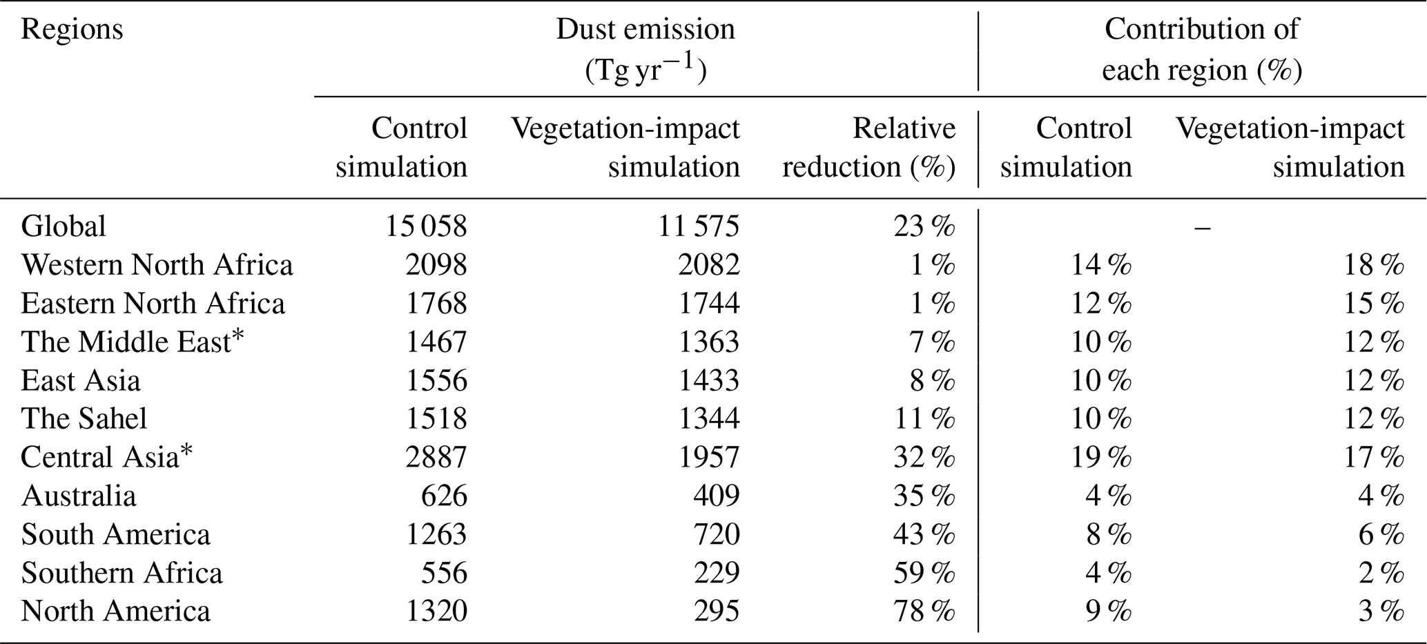
^* Note: To provide a more detailed regional characterization, the Middle East and central Asia (originally aggregated in Kok et al. (2021a), Fig. S5) were differentiated: The Middle East is defined as the region situated south of 40° N and west of 60° E, and the remaining areas of the original domain, are categorized as central Asia.

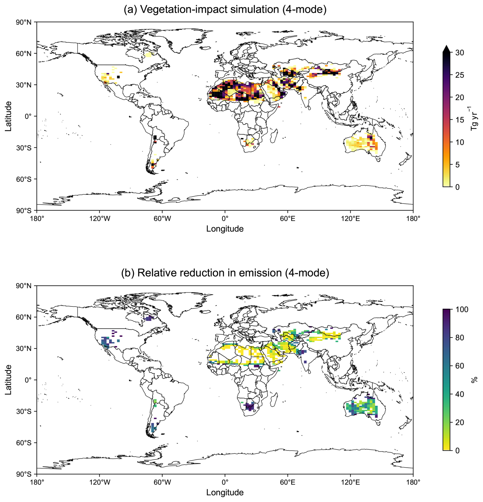
Figure 3 Simulated global dust emission fluxes and the vegetation-induced relative reduction in 4-mode configuration. (a) Mean annual dust emission flux (Tg yr⁻¹) in the vegetation-impact simulation. (b) Relative reduction in dust emission (%) due to vegetation effects, calculated as (control − vegetation-impact)$/$control.

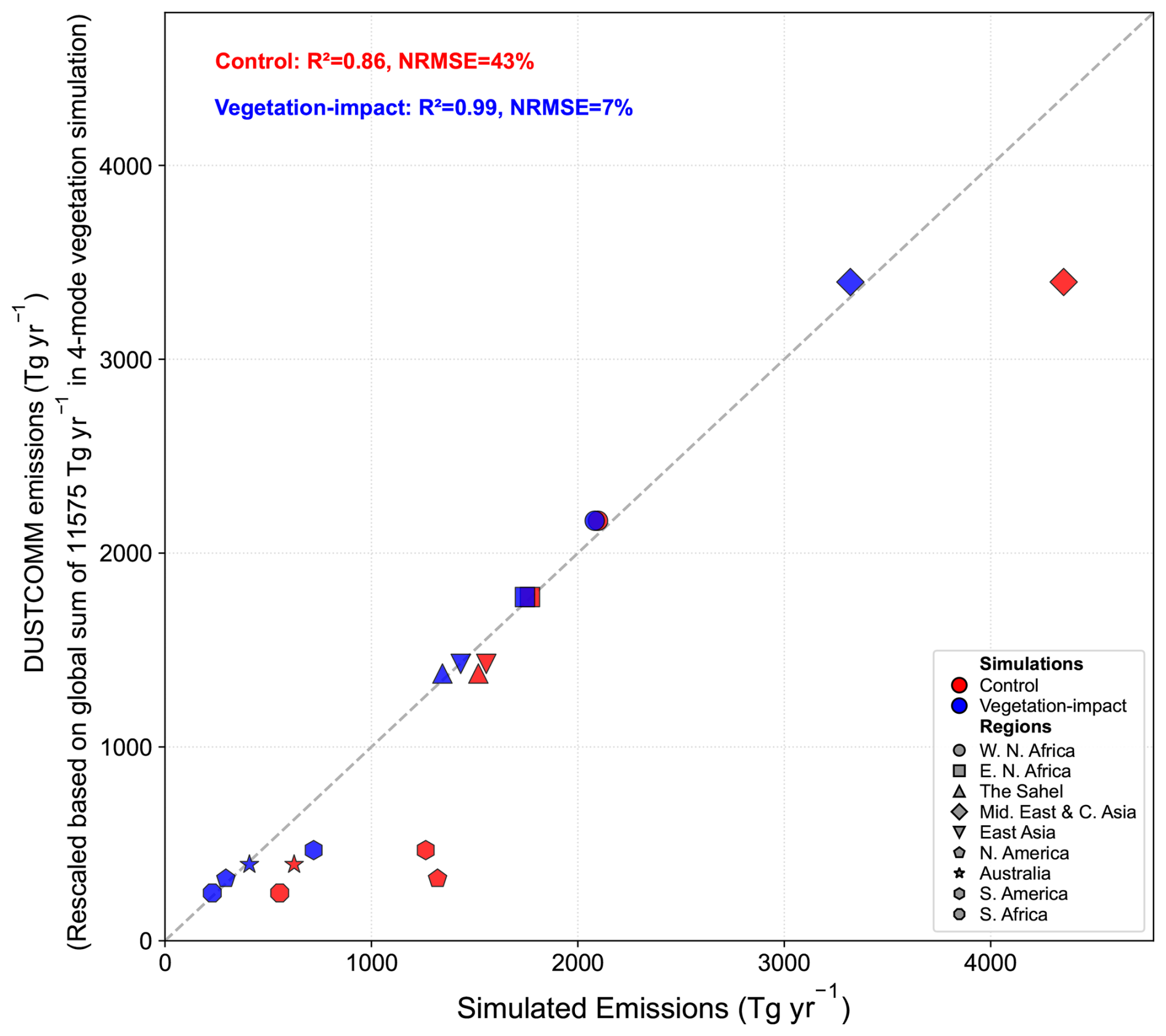
Figure 4 Comparison of simulated regional dust emissions (x-axis) against the DustCOMM emission by Kok et al. (2021b) (y-axis) in 4-mode configuration. The rescaling factors were applied to both the control (red) and vegetation-impact (blue) simulations. The DustCOMM emissions were rescaled to the global total emissions in the vegetation-impact simulation. The 1:1 line (dashed), R², and NRMSE are provided for reference.

3.2 DAOD under different vegetation treatments and particle size representations

Through the a posteriori application of the global scaling coefficients (Sect. 2.3.3) to the monthly history files, the adjusted global mean annual DAOD values were 0.031 for the control and 0.025 for the vegetation-impact simulations for both size-mode configurations (Figs. 5, S17). All subsequent analyses were conducted using these offline-adjusted results.

Regions with the largest DAOD can be found over western North Africa, central and East Asia, encompassing the Sahara, Kyzylkum, and Gobi Deserts (Alsharif et al., 2020) (Figs. 5a, S17a, b, d). The global maximum over Northern Africa is a common feature of global dust studies (Ridley et al., 2016; Song et al., 2021; Leung et al., 2024). Furthermore, the prominent hotspots in central and East Asia were consistent with several modelling studies (Zender et al., 2003; Ridley et al., 2016), although the model LMDzORINCA showed more prominent features in these regions compared to other dust schemes (e.g., Kok et al., 2014; Leung et al., 2024).

The relative difference map (Figs. 5b, S17c) clearly revealed the strong regional heterogeneity in DAOD reduction arising from the incorporation of vegetation effect. Globally, the mean annual DAOD decreased by 19 % when shifting from the control to the vegetation-impact simulations in both size-mode configurations (Tables S5, S6). A major reduction in DAOD was observed over the Thar Desert in north-western India. This region which constituted a major DAOD hotspot in the control simulation (Fig. S17a, d), showed a significantly reduced contribution when vegetation was accounted for (Figs. 5a, S17b). Such a reduction was directly attributed to the substantial suppression of dust emissions by the vegetation across this region (Figs. 3b, S7d). Furthermore, the result that the Thar Desert does not constitute a major DAOD hotspot is also supported by numerous other published works based both on observations and simulations (Zender et al., 2003; Kok et al., 2014; Ridley et al., 2016; Pandey et al., 2017; Leung et al., 2024).

The reduction in DAOD was also pronounced over North America, southern Africa, South America, and Australia, ranging from 34 % to 71 % (Tables S5, S6). In contrast, (hyper-)arid regions such as western and eastern North Africa and the Sahel experienced much more limited reductions of only 3 %–6 %, while moderate declines of 10 %–20 % were noted in the Middle East, central and East Asia (Tables S5, S6). The regional relative reductions in DAOD due to the effect of vegetation showed a significant correlation with the reductions of dust emissions (R²=0.97 for both the 1-mode and 4-mode configurations) based on the data in Tables S5 and S6.

Analysis of the 4-mode configuration revealed that Mode 2 (MMD = 2.5 µm) and Mode 3 (MMD = 7 µm) dominate the contributions of the modes to DAOD. In the control simulation (Fig. S18), these two modes contributed equally, each accounting for 42 % of the total DAOD. When accounting for the effects of vegetation (Fig. S19), the comparison between the control and vegetation-impact simulations (Fig. S20) indicated that Mode 3 experienced a slightly stronger reduction than Mode 2. This likely reflects the non-linear sensitivity of DAOD to changes in emissions due to vegetation effects across different particle size ranges. Consequently, this shift led to a redistribution of the modal proportions, with Mode 2 increasing to 44 % and Mode 3 decreasing to 40 % of the total DAOD in the vegetation-impact simulation (Fig. S19).

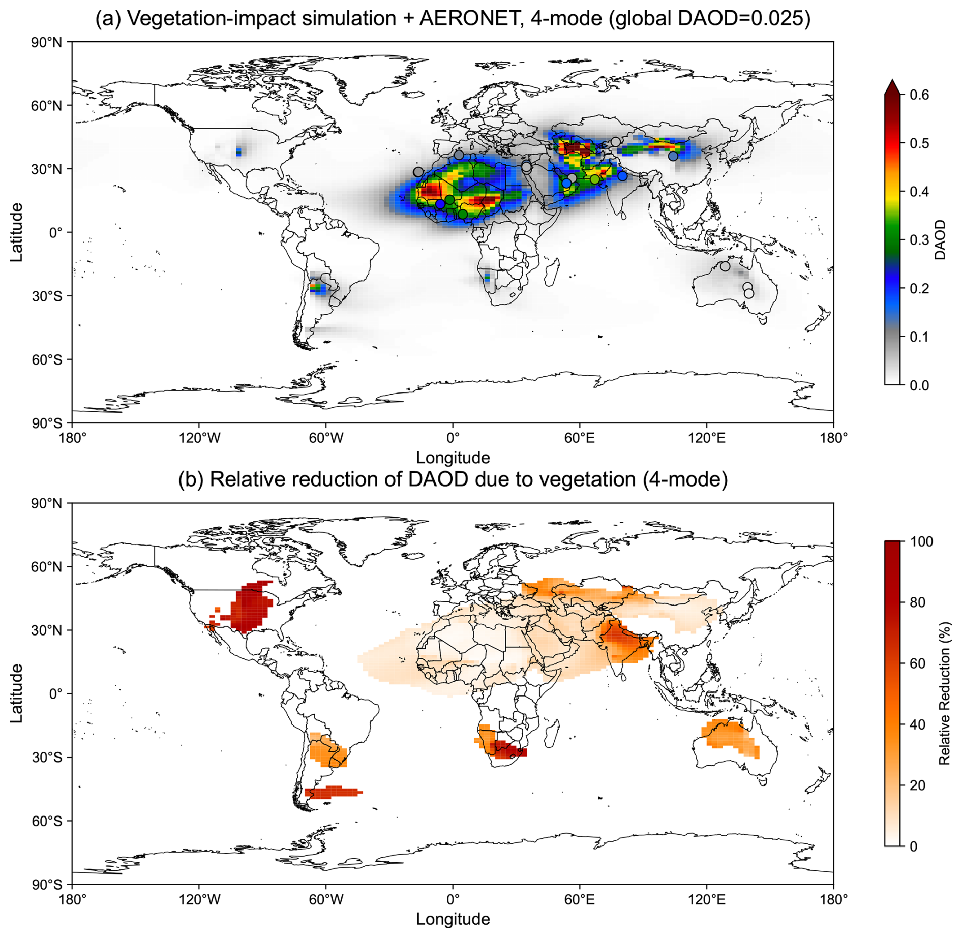
Figure 5 Spatial distribution of mean annual dust aerosol optical depth (DAOD) at 550 nm in 4-mode configuration. Panel (a) shows the vegetation-impact simulation with the global mean annual DAOD labelled; markers represent AERONET-SDA observations for comparison. Panel (b) shows the relative reduction in DAOD due to vegetation effects, calculated as (control − vegetation-impact)$/$control, with only grid cells exhibiting DAOD ≥ 0.05 in the control simulation displayed to ensure physical relevance and consistency with panel (a). All simulations incorporate DAOD-based scaling coefficients to match the observation-based target range of 0.030 ± 0.005.

To evaluate simulated DAOD, we compared the model results against observations from dust-dominant AERONET-SDA sites (locations shown in Figs. 2a, 5a), displaying only data points where the relative difference between the control and vegetation-impact simulations exceeded 3 %, in order to emphasize regions sensitive to vegetation impacts (Fig. 6). In the control simulations, an overall overestimation was observed, with the majority of data points falling below the 1:1 line – indicating that simulated values (x-axis) exceeded observed values (y-axis) (Fig. 6a, c). In contrast to the control simulation (Fig. 6c), the vegetation-impact simulation (Fig. 6d) in the 4-mode configuration showed an improved regression slope, increasing from 0.61 to 0.73, but a slight improvement in the correlation (R² increased from 0.67 to 0.68, while the RMSE decreased from 0.10 to 0.07, and the MB dropped from 0.06 to 0.03, representing a 50 % reduction) (Table S3). The similar tendencies can be seen with the 1-mode configuration, which showed an increase in the regression slope and reductions in RMSE and MB, despite a minor decrease in R² from the control (Fig. 6a) to vegetation-impact simulation (Fig. 6b). Overall, the vegetation-impact simulations mitigated overestimations present in the control simulations, yielding the regression slopes closer to unity and reducing systematic bias (Fig. 6b, d, Table S3). Specifically, the effect of vegetation was more pronounced over the following areas: Thar Desert, Australia, Taklamakan, and the Mali/Niger. For example, the observed mean annual DAOD over the Thar Desert for the year 2008 was 0.18, whereas the model behaviour transitioned from a pronounced overestimation in the control simulation (0.25, 0.37 in 1-mode and 4-mode, respectively) to a slight underestimation in the vegetation-impact simulation (0.13, 0.15 in 1-mode and 4-mode, respectively).

In addition to the AERONET-SDA comparison, we also evaluated seasonal DAOD averaged over 15 regions against the observationally based model constraints from Kok et al. (2021a), with only data points exceeding a 3 % relative difference shown in Fig. 7. In both the 1-mode and 4-mode configurations, the vegetation-impact simulations (Fig. 7b, d) exhibited better performance compared to the control simulations (Fig. 7a, c), with higher R² values, lower RMSE and MB. Noticeably, the regression slope increased from 0.56 (control) to 0.68 (vegetation-impact) in the 1-mode configuration and from 0.50 (control) to 0.63 (vegetation-impact) in the 4-mode configuration. These shifts toward the 1:1 line suggest that incorporating vegetation effects provides a more physically consistent representation of regional and seasonal DAOD.

Significant regional improvement was observed in the Thar Desert during summer (JJA) with Indian Summer Monsoon, where the simulated DAOD dropped from 0.62 (1-mode) and 0.71 (4-mode) in the control simulations to 0.35 (1-mode) and 0.36 (4-mode) in the vegetation-impact simulations, respectively, closely approaching the observational constraint of 0.32. This pattern of DAOD also corresponded well with the simulated reduction in dust emissions over north-western India (Fig. 3b). Similarly, in the Taklamakan Desert – a major global dust source – DAOD during JJA decreased from 0.26 (1-mode) and 0.27 (4-mode) in the control to 0.19 (both 1-mode and 4-mode) in the vegetation-impact simulations, compared to the observationally constrained value of 0.17 (Fig. 7).

Several seasonal and regional discrepancies in the simulated DAOD were evident (Fig. 7), suggesting that regional emission rescaling alone cannot fully compensate for structural deficiencies in transport and meteorological representations. Underestimations occurred in both major source regions such as Mali/Niger, Bodele/Sudan and southern Middle East, as well as downwind regions, including the African West Coast and mid-Atlantic primarily during JJA. These biases likely reflect deficiencies in simulating monsoon dynamics and associated convective processes, due to decoupling of dust–radiation interactions and unresolved sub-grid-scale haboob events (Pope et al., 2016; Balkanski et al., 2021; Bergametti et al., 2022). By contrast, the overestimations in the Kyzyl Kum and Gobi deserts during MAM and JJA might reflect insufficient long-range transport efficiency, leading to excessive near-source accumulation. Furthermore, the underestimation in the Taklamakan Desert suggests limitations in representing vertical lofting and atmospheric stability within topographically enclosed basins (Nan and Wang, 2018). A more detailed discussion of model–observation discrepancies is provided in Sect. S2 in the Supplement.

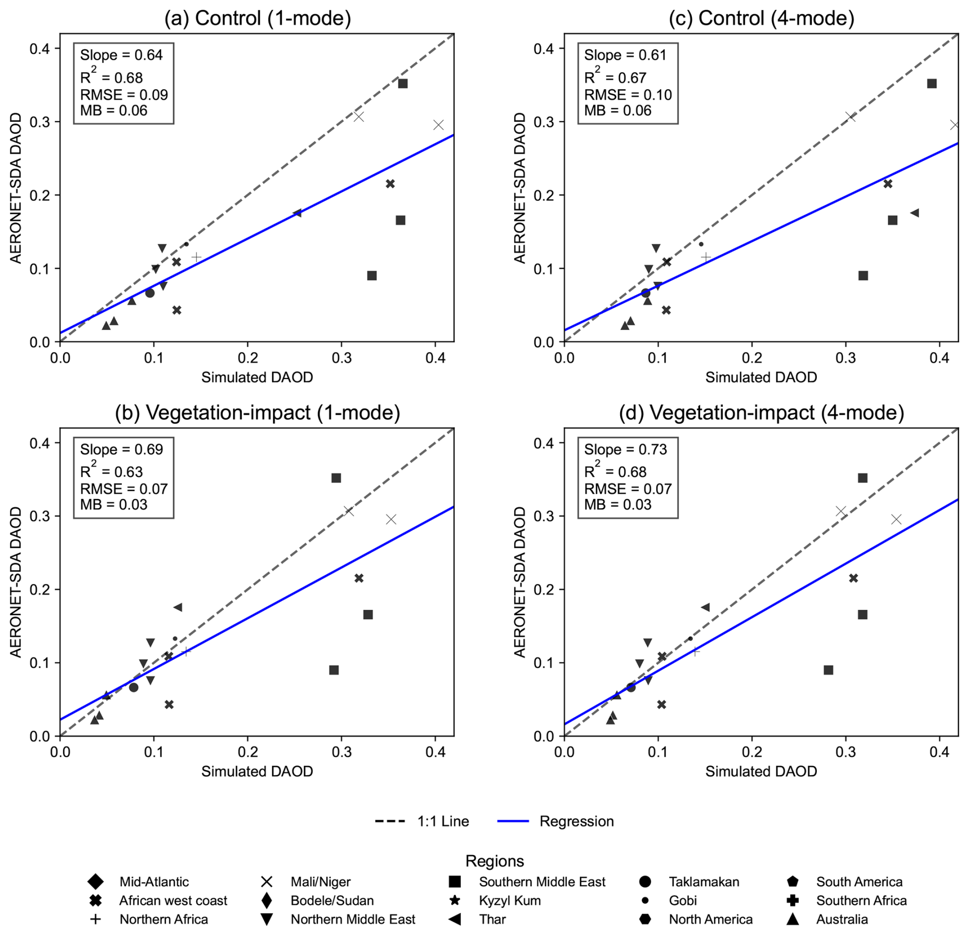
Figure 6 Evaluation of mean annual simulated DAOD at 550 nm against AERONET-SDA observations. Panels compare results from the control simulations (without vegetation effects; a, c) and the vegetation-impact simulations (b, d). The left column (a–b) illustrates the performance of the 1-mode configuration, while the right column (c–d) provides a comparative analysis of the 4-mode configuration. Different regions are represented by different marker shapes, with the best-fit line shown in blue and the 1:1 reference line shown as a black dotted line. The statistical metrics (R², RMSE, and MB) and the slope of the regression line are given in each subplot. Only points with a relative difference exceeding 3 % between the control and vegetation-impact simulations are included to emphasize regions sensitive to vegetation impacts.

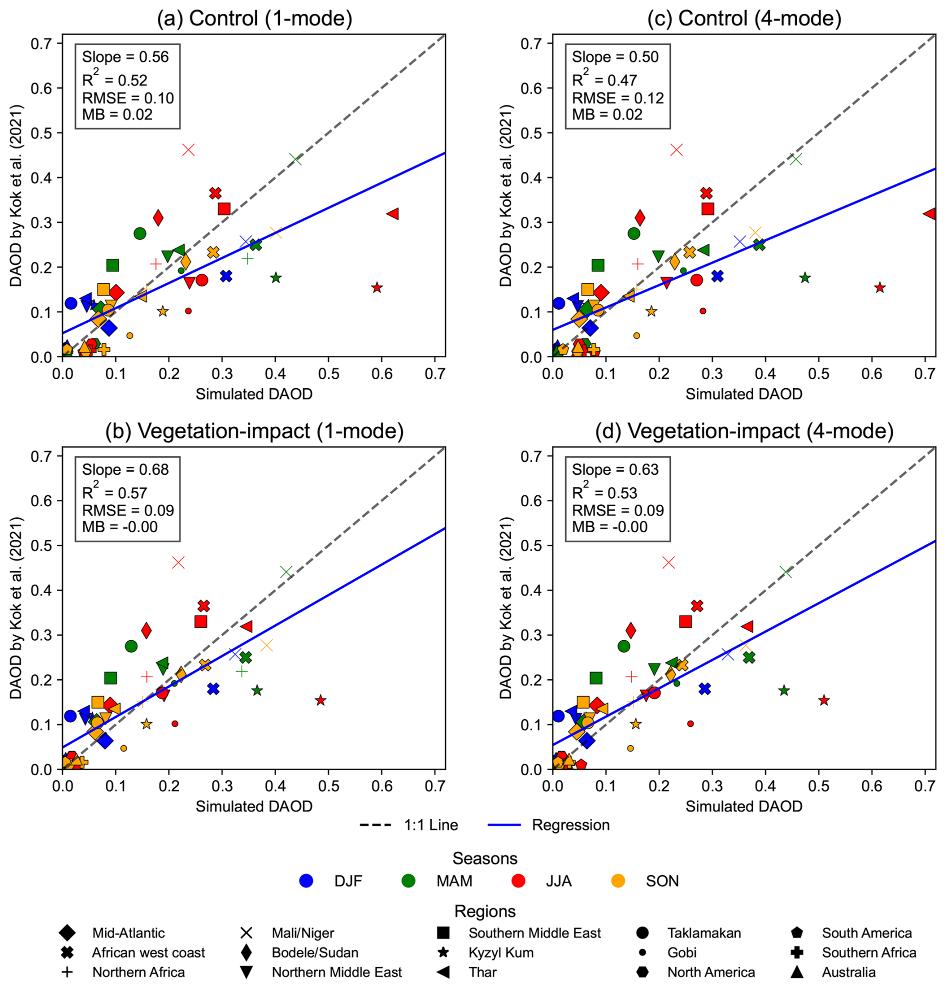
Figure 7 Evaluation of simulated DAOD at 550 nm against observationally constrained DAOD by Kok et al. (2021a) based on averages over 15 regions. Panels compare results from the control simulations (without vegetation effects; a, c) and the vegetation-impact simulations (b, d). The left column (a–b) illustrates the performance of the 1-mode configuration, while the right column (c–d) provides a comparative analysis of the 4-mode configuration. The coefficient of determination (R²), RMSE, MB and slope are shown in each subplot. Different regions are represented by different marker shapes, while the four seasons (DJF: December, January, and February; MAM: March, April, and May; JJA: June, Jul, and August; SON: September, October, and November) are distinguished by different colours. The best-fit line is shown in blue, and the 1:1 reference line is shown as a black dotted line. Only points with a relative difference exceeding 3 % between the control and vegetation-impact simulations are included to emphasize regions sensitive to vegetation impacts.

3.3 Surface PM concentration from dust: spatial variability and evaluation against observations

We analysed the impact of vegetation on the dust cycle by comparing the simulated near-surface dust particulate matter (PM) concentrations (µg m⁻³) between the control and vegetation-impact simulations. This metric, representing the mass of dust aerosol per unit volume of air, serves as a critical indicator of regional air quality and is a critical measurement to characterize the dust cycle.

Both size-mode configurations reproduced major global dust hotspots over North Africa, the Middle East, central and East Asia, Australia, and southern Africa, as well as the adjacent oceans (Figs. 8a, S21a, b, d). Incorporating vegetation led to a global reduction in surface dust concentrations by 17 % (1-mode; Table S5) and 19 % (4-mode; Table S6), exhibiting a distinct spatial pattern (Figs. 8b, S21c). The most prominent reduction occurred in hotspots located in North and South America, north-western India, southern Africa, and Australia, as well as far-field downwind pathways, including the Atlantic Ocean off the south-eastern coast of South America, Indian Ocean off the eastern coast of South Africa, and the Pacific Ocean off the western coast of North America. As expected, the regional relative reductions in surface PM concentration showed a high correlation with the regional relative reductions in dust emissions (R²=0.98 for both configurations), based on the data in Tables S5 and S6. The 4-mode configuration (Figs. 8, S21d) exhibited a more widespread dust distribution and substantially stronger PM reduction than the 1-mode (Fig. S21a–c). This increased spatial extent stems from the broader size spectrum inherent in the 4-mode scheme, enabling a more comprehensive representation of size-dependent emission, transport, and settling processes.

A detailed comparison between the two size-mode configurations (Fig. S21e–h) showed that the 4-mode configuration produced higher surface concentrations over primary source regions – such as North Africa, central and East Asia, and Australia – and their immediate downwind oceans. Conversely, over the more remote regions from emissions such as the tropical Pacific and Indian Oceans, northern South America, and Southeast Asia, the 1-mode configuration exhibited higher concentrations in these areas compared to the 4-mode configuration. This discrepancy is primarily due to the higher emissions in Mode 2 (MMD = 2.5 µm) in the 1-mode configuration (1243 Tg yr⁻¹ in the vegetation-impact simulation) compared to its contribution in the 4-mode configuration (565 Tg yr⁻¹ in the vegetation-impact simulation), which results in a greater proportion of fine dust available for long-range transport.

Figure 9 presents the evaluation of simulated dust PM₁₀ concentrations in 4-mode configuration against fixed-point observations (Mahowald et al., 2009; site locations exhibited in Figs. 2b and 8a). Across all simulations, the majority of data points remained within one order of magnitude of the observations. Accounting for vegetation effects led to a modest improvement in spatial correlation between the model and observations (Fig. 9), which is likely related to the spatial distribution of observational sites (Figs. 2b and 8a). Most surface PM concentration sites (Fig. 2b) are located in regions spatially distant from areas where vegetation-induced emission changes are most pronounced. As a result, vegetation-driven signals are strongly diluted during transport and mixing, leading to a weaker sensitivity in surface PM concentrations. In contrast, a larger proportion of AERONET-SDA (DAOD) sites (Fig. 2a) are situated in or near dust source and transition regions (e.g., the Thar Desert), where vegetation effects are more directly reflected in column-integrated dust loading. Consistently, dust deposition observations, which span both source and remote regions (Fig. 2c), show more pronounced vegetation-induced improvements over land than over ocean (Sect. 3.4), indicating that vegetation sensitivity is modulated by the spatial representativeness of observations.

For data points sensitive to vegetation effects (those with a relative difference greater than 5 %), the spatial correlation (R(log)) slightly improved from 0.91 to 0.92, the RMSE (log) slightly decreased from 0.51 to 0.49, and the MB (log) shifted from 0.15 in the control to 0.03 (representing an 80 % reduction) in the vegetation-impact simulation (Table S3). This shift indicated that the vegetation mitigated the systematic overestimations inherent in the control simulation, bringing surface concentrations slightly closer to the values from site-based observations. Specific improvements were observed over sites of North America/Arctic, Africa, and Oceania with relative differences between control and vegetation-impact simulations exceeding 20 %; in these regions, the simulated overestimations shifted closer to the 1:1 line (Fig. 9).

Despite these improvements, the simulations in both size-mode configurations (Figs. 9, S22) consistently underestimated surface PM concentrations by approximately one order of magnitude in East Asia, with an even stronger underestimation in the 4-mode configuration over the Pacific than the 1-mode configuration (Fig. S22). As these sites are located in downwind regions, the discrepancies likely reflect uncertainties in long-range transport representation in the model (Uno et al., 2009) and potential contamination from anthropogenic aerosols in the observations (Prospero and Savoie, 1989; Chuang et al., 2005). Similar discrepancies relative to observations are also evident in the results of Leung et al. (2024). Further details regarding these model–observation discrepancies are provided in Sect. S3.

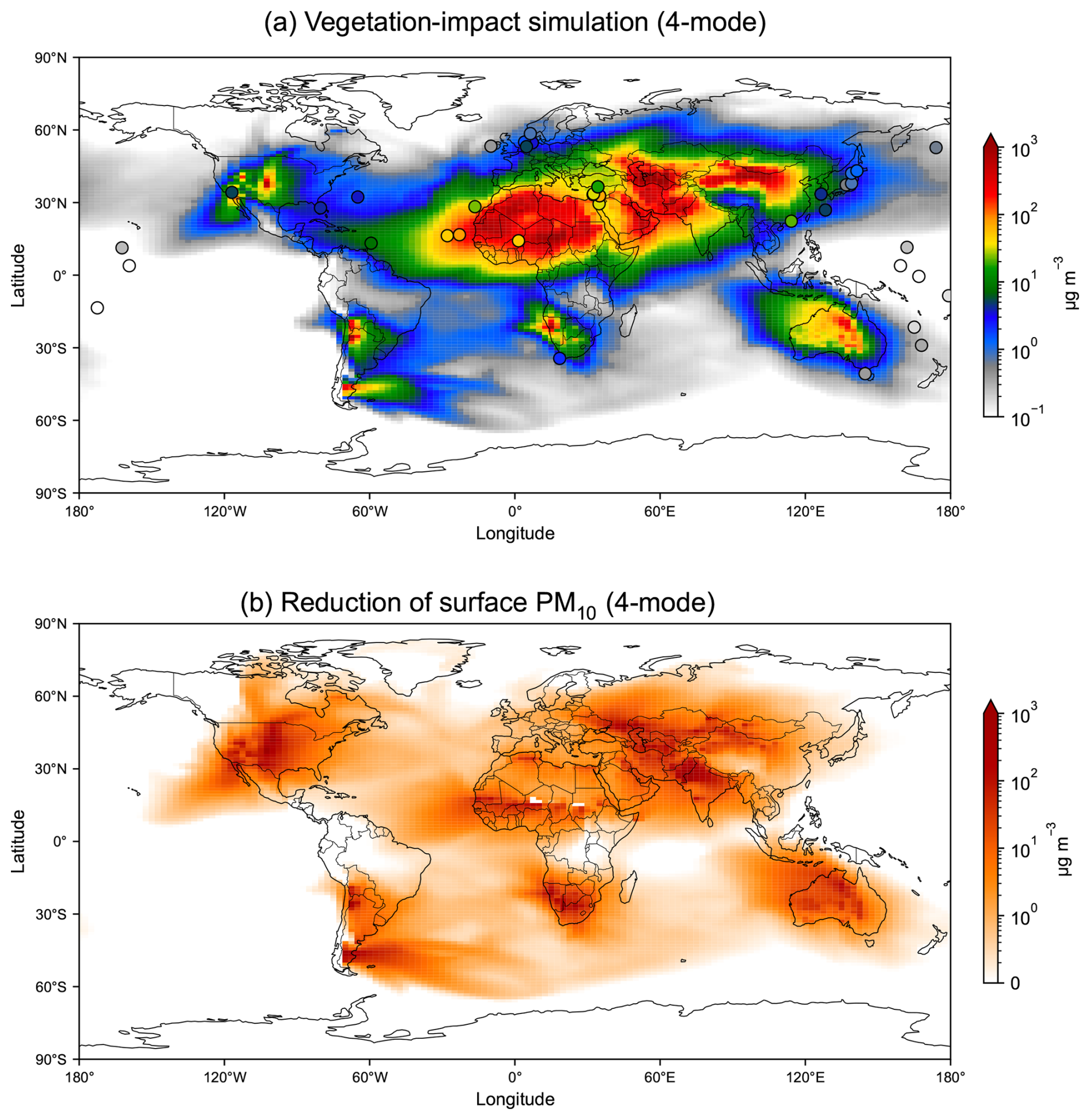
Figure 8 Spatial distribution of surface PM₁₀ concentration (µg m⁻³) in the 4-mode configuration. Panel (a) shows the mean annual dust PM₁₀ concentration in the vegetation-impact simulation, overlaid with markers representing the observational locations of Mahowald et al. (2009). Panel (b) shows the reduction in mean annual PM₁₀ concentration due to vegetation effects, calculated as control − vegetation-impact.

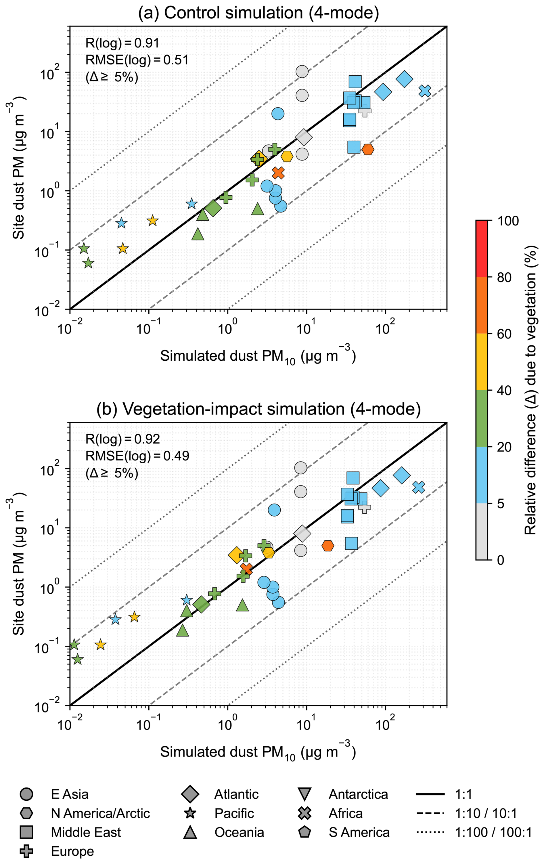
Figure 9 Evaluation of simulated and observed dust surface PM₁₀ concentration (µg m⁻³) by Mahowald et al. (2009) in the 4-mode configuration. Panels (a) and (b) show the control and vegetation-impact simulations, respectively. Both axes are plotted on logarithmic scales. Different regions are indicated by different marker shapes, with colours in each plot representing the relative difference between the control and vegetation-impact simulations. Statistical metrics (R and RMSE, computed in log space) are shown in each panel and calculated only for data points with relative differences (Δ) greater than or equal to 5 %, highlighting regions sensitive to vegetation impacts. The solid black line denotes the 1:1 relationship. The inner dashed lines indicate the 10:1 and 1:10 ratios, representing simulated values within one order of magnitude of the observations, while the outer dashed lines represent two orders of magnitude (100:1 and 1:100 ratios). Some observational sites are not visible because their values fall below the lower axis limits.

3.4 Dust surface deposition: spatial variability and evaluation against observations

We analysed here the simulated dust surface deposition in different model configurations and compared them to observations.

The highest simulated total dust deposition occurred near major source regions, including North Africa, central and East Asia, further extending to downwind terrestrial and oceanic regions, such as the Atlantic and Indian Oceans (Figs. 10a, S23a, b, d). The 4-mode configuration (Figs. 10a, S23d) exhibited more intense dust deposition with wider spatial coverage than the 1-mode (Fig. S23a, b), with higher total deposition across most continental and proximal oceanic regions, particularly in areas near major dust sources (Fig. S23e–h). Conversely, lower deposition values in the 4-mode configuration – relative to 1-mode configuration – were observed in remote downwind regions. Notably, these spatial patterns of dust deposition aligned closely with the simulated dust surface concentrations (Figs. 8, S21), due to rapid gravitational settling near source regions and limited long-range transport resulting from the explicit representation of coarse particles in the 4-mode configuration.

The difference in deposition between the control and vegetation simulations (Figs. 10b, S23c) exhibited many features in common with the changes in PM₁₀ (Figs. 8b, S21c). Total surface dust deposition was reduced by 23 % globally across both size-mode configurations due to the inclusion of vegetation (Tables S5 and S6). As expected, the most pronounced deposition changes mapped onto the regions where vegetation caused an emission decrease, including India, North and South America, southern Africa, and Australia. Notable reductions also extended to downwind oceanic regions. Based on Tables S5 and S6, the regional relative decline in surface deposition was highly correlated with and largely proportional to the reductions in emissions, DAOD and surface concentrations (R²≥0.96 for both the 1-mode and 4-mode configurations).

Regarding the differences among individual deposition processes, dry deposition and sedimentation in both the control (Figs. S24b–c, S25b–c) and vegetation-impact simulations (Figs. S24e–f, S25e–f) were largely confined to source regions characterized by higher dust mass fluxes. In contrast, wet deposition (Figs. S24a, d, S25a, d) extended much farther from continental source regions to remote oceanic areas, albeit with lower absolute mass fluxes. The differences between the control and vegetation-impact simulations were spatially more widespread and exhibited larger reductions for wet deposition than for the other deposition processes (Figs. S24g–i, S25g–i), particularly in downwind marine regions such as the Atlantic and Indian Oceans. This suggests that vegetation-induced changes in dust emissions affect the deposition occurring all along long-range transport pathways, over both continental and remote marine environments.

Evaluation against the observational total dust deposition dataset (Albani et al., 2014; site locations in Figs. 2c and 10a) indicated that incorporating vegetation effects enhanced spatial correlation and reduced bias compared to the control simulations (Figs. 11, S26; Table S3). For data points where the relative differences between the two simulations were greater than or equal to 5 %, the inclusion of vegetation effects slightly increased R (log) from 0.77 to 0.80 and decreased RMSE (log) from 0.96 to 0.87 in the 4-mode configuration, and decreased MB (log) from 0.36 to 0.19 (representing a 47 % reduction) (Fig. 11, Table S3). Compared to the control simulation, persistent overestimations were mitigated in the vegetation-impact simulation, with relative differences exceeding 40 %, shifting simulated values closer to the 1:1 reference line in regions such as North America, East Asia, and Antarctica. In particular, the reduced positive bias of dust deposition over Antarctica reflected the decreased dust emissions primarily originating from South America (Patagonia), Australia, and southern Africa (Li et al., 2008; Neff and Bertler, 2015). Due to vegetation effects, integrated emissions south of 30° S were reduced by approximately 60 %, indicating that adjustments in emissions from these shared source regions can substantially influence the Antarctic dust budget (Neff and Bertler, 2015). The persistent overestimation of deposition in Antarctica is discussed in Sect. S4. Additionally, the majority of data points fell within the 1:100–100:1 range, whereas two to three Pacific sites remained outside these bounds, exhibiting a persistent underestimation of dust deposition.

Analysing the deposition sites over land and over ocean domains separately revealed that the model captured dust deposition better over the land compared to the ocean for both model configurations (Figs. S27–S28). The inclusion of vegetation effects led to a more substantial reduction in RMSE over land than over oceanic regions. This suggests that vegetation-driven emission constraints exert a more direct influence on terrestrial dust deposition, whereas oceanic regions are more affected by uncertainties in the representation of long-range transported particles (Uno et al., 2009).

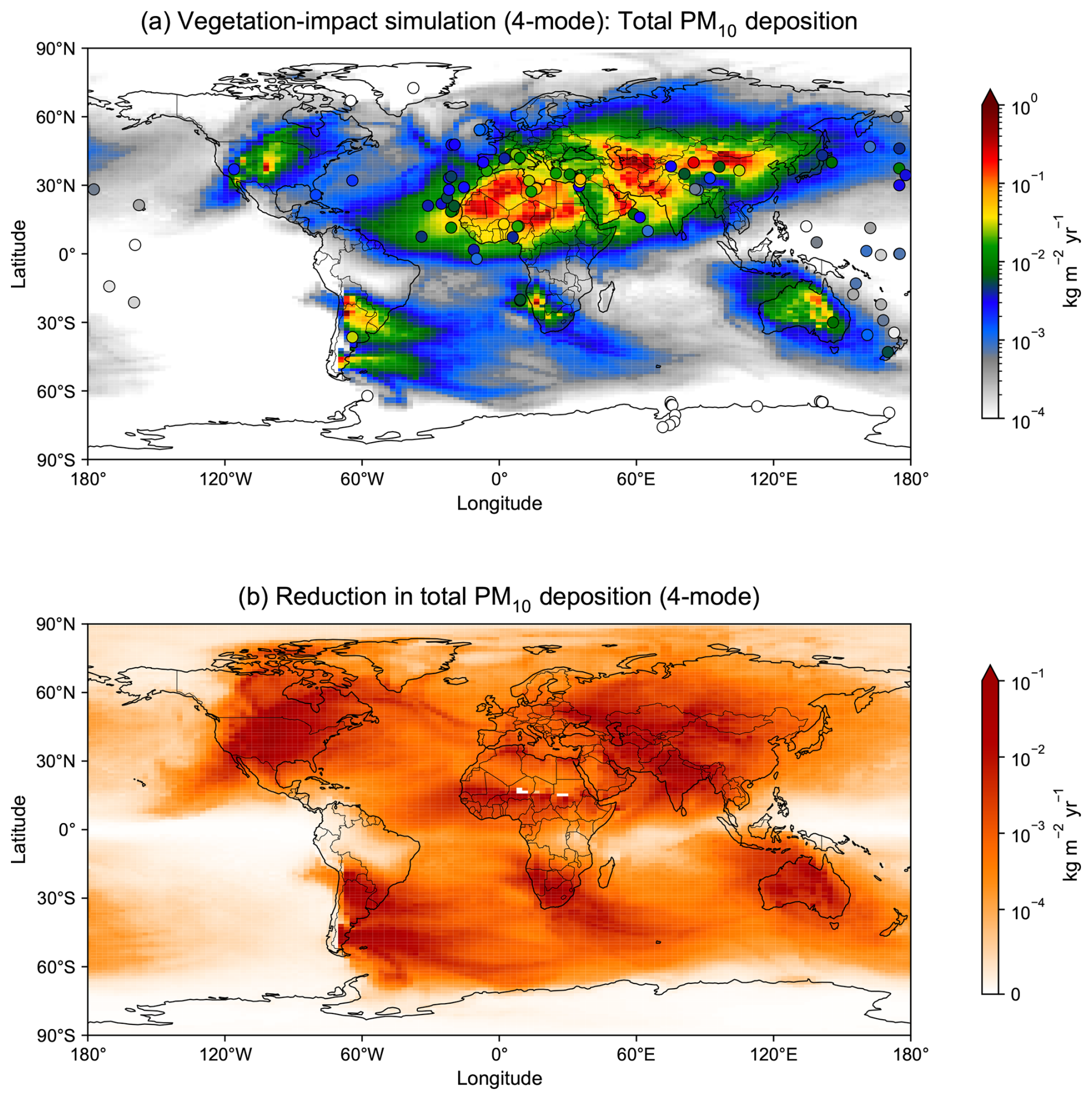
Figure 10 Spatial distribution of mean annual dust surface PM₁₀ total deposition (kg m⁻² yr⁻¹) in the 4-mode configuration. Panel (a) shows the dust PM₁₀ total deposition in the vegetation-impact simulation, overlaid with markers representing the observational locations of Albani et al. (2014). Panel (b) shows the reduction in PM₁₀ total deposition due to vegetation effects, calculated as control − vegetation-impact.

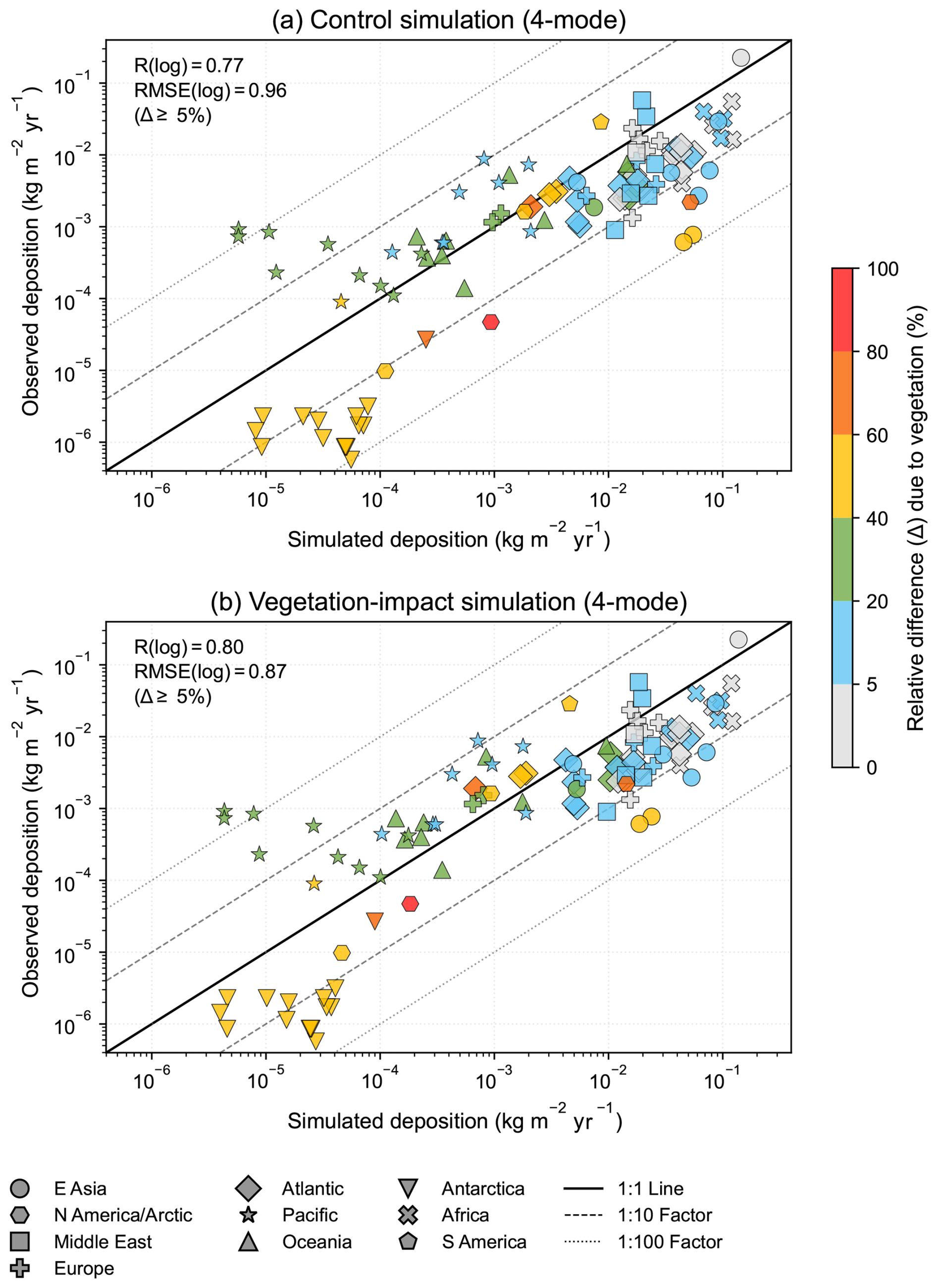
Figure 11 Evaluation of simulated and observed dust surface PM₁₀ total deposition (kg m⁻² yr⁻¹) by Albani et al. (2014) in the 4-mode configuration. Panels (a) and (b) show the control and vegetation-impact simulations, respectively. Both axes are plotted on logarithmic scales. Different regions are indicated by different marker shapes, with colours representing the relative difference between the control and vegetation-impact simulations. Statistical metrics (R and RMSE, computed in log space) are shown in each panel and calculated only for data points with relative differences (Δ) greater than or equal to 5 %, highlighting regions sensitive to vegetation impacts. The solid black line denotes the 1:1 relationship. The inner dashed lines indicate the 10:1 and 1:10 ratios, representing simulated values within one order of magnitude of the observations, while the outer dashed lines represent two orders of magnitude (100:1 and 1:100 ratios). Some observational sites are not visible because their values fall below the lower axis limits.

3.5 Uncertainties and limitations in simulating the global dust cycle

We now discuss the improvement that can be brought in the future by identifying key limitations and the causes of the uncertainties in both the modelling framework and model–observation comparisons.

Several limitations emerge in the current dust emission scheme with explicit consideration of vegetation. First, in relation to surface roughness, the threshold velocity was recomputed based on vegetation-related roughness while applying a constant, minimal value for non-vegetation elements (e.g., pebbles, rocks) based on Foroutan et al. (2017). In reality, the aerodynamic effects of these solid elements are dynamic and spatially heterogeneous (Leung et al., 2023), suggesting that future studies could incorporate a more spatially resolved parameterization of non-vegetative roughness to better capture its impact on the wind stress partition. In addition, because threshold velocity depends on near-surface soil properties and soil erodibility is a key control on dust emissions, future developments could more explicitly incorporate soil texture (e.g., clay fraction) to improve the physical realism of the scheme (Balkanski et al., 2021).

Second, the seasonal variations of vegetation density influence how the seasonality of dust is represented. However, due to a poor description of grassland phenology in the ORCHIDEE model, the seasonal variations of the fraction of vegetation cover (A_v) are insufficiently captured (Xu et al., 2026). The limitation of A_v seasonality propagates to the threshold velocity (u_t) in our framework, thereby affecting the seasonal variation of dust emissions and the broader dust cycle (Figs. S9, S10). The pronounced reduction in dust emissions observed during specific periods, despite weak seasonal variability in simulated vegetation cover, may reflect a state-dependent sensitivity of dust flux to vegetation. This sensitivity was likely modulated by the mean meteorological conditions; for example, in the Sahel, increased precipitation and subsequent surface moistening during summer acted synergistically with vegetation to amplify the suppression of dust emissions. These mechanisms warrant further investigation, and addressing this limitation could improve future representations of dust emission.

Third, the current dust emission scheme that couples dust emission to the vegetation state does not differentiate among vegetation types (e.g., trees, crops, and grasses) and their distinct structural characteristics. Currently, the dust suppression mechanism we apply only accounts for gaps of bare soil within grasslands rather than gaps for all vegetation types. We employed this simplification because dust emissions primarily occur in (semi-)arid regions, which are largely dominated by grassland (Allaby, 2006; Shinoda et al., 2011; Blair et al., 2013), making it the most critical vegetation type to parameterize for natural dust cycles. While cropland gaps can be important sources of anthropogenic dust due to agricultural disturbances (Chen et al., 2018), the present study focuses exclusively on natural mineral dust processes, justifying their current exclusion. It should also be noted that dust emission from forest gaps is physically much more constrained, as the high canopy sheltering effect necessitates substantially higher wind energy to initiate emission (Breshears et al., 2003). Consequently, these diverse vegetation effects were simplified into a uniform treatment within the current framework. Future work could enhance the model's physical realism by distinguishing the unique suppressive effects of various biomes and by explicitly incorporating the gap structures inherent to forests and croplands.

The inclusion of vegetation cannot fully address the biases inherent in the model, as our evaluation of emissions without the regional rescaling factors (Sect. 2.3.2) reveals systematic discrepancies relative to DustCOMM (Figs. S13, S15, and S16). These discrepancies likely arise from several structural limitations in the model. First, the constraints for defining dust source areas are simplified. For instance, the use of a January temperature threshold – originally designed for Northern Hemisphere sources – may not fully capture the seasonal freezing cycles in the Southern Hemisphere. While this simplification does not affect our assessment of vegetation-induced effects (due to the methodological consistency across all simulations), it contributes to regional biases that we aim to address in future versions through a full month-by-month temperature check. Furthermore, the use of a 300 mm annual precipitation threshold (Schulz et al., 2009) may lead to inherent underestimations in semi-arid regions where episodic dust events occur despite higher mean annual precipitation (Huang et al., 2014; Khusfi et al., 2020). Second, structural biases in the nudged meteorological fields, particularly in the regional representation of surface wind speed, likely contribute to these discrepancies. Finally, the lack of fine-scale surface information, along with simplifications in land-surface properties (e.g., representation of non-vegetative roughness, such as rocks and pebbles), may also contribute to these systematic biases. While the relative importance of these factors varies across regions, their combined effect leads to systematic biases in emission magnitude and spatial distribution. Regional rescaling is therefore applied to provide an observational constraint on simulated emissions. Addressing these biases remains an important direction for future model development.

Different particle size representations provide complementary insights into reproducing DAOD. Despite the overall similar statistical performance of the 1-mode and 4-mode representations, their internal dust distributions differ substantially (Di Biagio et al., 2020). The 1-mode configuration concentrates mass into the fine mode (MMD = 2.5 µm), which possesses higher light scattering efficiency and a longer atmospheric lifetime due to lower deposition velocities (van der Does et al., 2016), contributing substantially (∼ 40 %) to total DAOD. By contrast, the 4-mode configuration distributes mass across a broader size range; consequently, the specific mode with an MMD at 2.5 µm accounts for a lower mass fraction compared to the 1-mode configuration, leading to distinct contributions to regional and global optical extinction.

Regarding the evaluation of model outputs against observations, several caveats underscore the limitations of current dust cycle simulations and available observational datasets. The scale mismatch between the model grid resolution of 2.5° × 1.27° and the localized measuring stations introduces a systematic bias in the comparison with in situ observations (Gliß et al., 2021). Furthermore, the coarse resolution limits the model's ability to resolve fine-scale meteorological processes that are critical for dust emission and transport, such as localized surface winds and nocturnal low-level jets. It also constrains the representation of complex orography, for example, in highly heterogenous alpine terrain, where steep elevation gradients and multiple peaks occur within a single grid cell. In contrast, the smoothed topography in coarse-resolution models assigns a uniform elevation to each grid cell, thereby suppressing orographic controls on dust mobilization and near-surface deposition. These limitations collectively hinder the accurate simulation of dust emission, transport and deposition processes (Ridley et al., 2013; Leung et al., 2024).

Additional caveats arise from uncertainties in the observational datasets. These include cloud contamination biases in cloud-screening algorithms, the potential misclassification of non-dust aerosol types in the AERONET-SDA DAOD product (Levy et al., 2010; Arola et al., 2017), and anthropogenic aerosol contamination in PM₁₀ observation (Prospero and Savoie, 1989; Chuang et al., 2005). Furthermore, the non-unified temporal coverage and inconsistent sampling protocols persist across surface concentration and deposition datasets compiled from different sources (Mahowald et al., 2009; Schulz et al., 2012; Albani et al., 2014; Ryder et al., 2018).

Finally, comparisons of simulated and observed dust surface concentrations and depositions highlight common deficiencies in global dust models regarding long-range transport efficiency of giant dust particles (Uno et al., 2009). In our simulations, the underestimation of dust deposition in remote downwind oceanic regions (e.g., the Pacific), contrasted with better agreement in near-source terrestrial regions (Fig. 11), suggests that the model likely underestimate particle lifetime due to overly rapid gravitational settling. Additional biases may also arise from under-resolved processes such as vertical lofting or uncertainties in regional source strength (Wu et al., 2020). These results underscore the necessity for improved representation of transport and removal processes to better capture the atmospheric lifetime and deposition of giant dust particles.

4 Conclusions and perspectives

This study points to the importance of the vegetation, in particular grassland, on modulating the dust cycle. By incorporating the vegetation data simulated by the ORCHIDEE land surface model into the LMDzORINCA dust emission scheme, we quantified the variations of emissions, DAOD, concentrations, and deposition due to the sheltering effects of vegetation. Building on our recent work (Xu et al., 2026), incorporating dynamic grassland densities provides an effective and feasible way to explicitly represent bare soil gaps within grasslands – a key control on dust emission. This allows for consistent estimates of vegetation characteristics from the ORCHIDEE model rather than getting information from external datasets (Foroutan et al., 2017; Klose et al., 2021; Leung et al., 2023). This study opens the way to fully couple vegetation to the dust cycle within the IPSL Earth System Model (Boucher et al., 2020). The next studies will hence focus on the feedbacks occurring in semi-arid regions between vegetation and dust cycle. It also opens the way to explore the role played by these interactions under climate change, extreme weather events, and potential tipping points.

The incorporation of vegetation reduces global dust emissions by 23 %, with higher reductions of 35 %–78 % in semi-arid regions, exhibiting the significant positive relationships between vegetation fraction and relative emission reduction across different regions. This modification alters the regional contribution of emissions to the global dust cycle: higher contributions take place from major dust source regions with sparse vegetation and lower contributions occur from regions where vegetation cover is more abundant. The suppressive effect of vegetation also reduces significantly global dust loads from the control simulation, both in source regions – such as the Thar Desert – and in remote downwind areas, including Antarctica, where total deposition is considerably reduced. Overall, evaluations against DAOD, surface concentration, and deposition observations show model improvements that vary from modest to significant depending on the region.

This study also investigates the impact of simulated dust particle size representations. The 4-mode representation provides a more comprehensive description of the dust particle size distribution, whereas the 1-mode representation, which is more computationally efficient, treats mainly micrometre-sized particles below 7 µm. The 1-mode distribution appears to adequately represent optical properties but provides a simplified representation of concentrations and deposition distributions. Models still struggle in their current state to represent coarse particles. This is manifest in the long-range transport, in overly rapid dry deposition, and in insufficient vertical lofting, which all contribute to the underestimation of surface concentrations and deposition fluxes in remote downwind regions. Taken together, these results demonstrate that accounting for vegetation effects and adopting an appropriate size-distribution framework are crucial for improving the physical consistency of dust simulations.

Building on these findings, we identify several priorities for future development: (1) Improving the representation of dust source restriction (e.g., temperature and precipitation thresholds) and surface roughness, including the distinct aerodynamic effects of different vegetation types, non-vegetative roughness elements (e.g., rocks and pebbles), and the seasonal variation of vegetation; (2) Moving toward higher spatial resolutions to better resolve sub-grid meteorological variability and orographic heterogeneity, supporting both more accurate simulation of dust processes and more robust evaluations against point-scale observational sites; (3) Improving the treatment of coarse particle dynamics in transport and deposition schemes, particularly gravitational settling and scavenging processes, to more accurately represent atmospheric residence times and long-range transport; and (4) Advancing fully coupled Earth System Model (ESM) frameworks that integrate climate, aerosols, and dynamic vegetation, enabling a more consistent representation of the bidirectional feedbacks between land-surface changes and the global dust cycle.