Global CO emissions and drivers of atmospheric CO trends constrained by MOPITT satellite measurements

Carbon monoxide (CO), an important atmospheric pollutant produced by incomplete combustion and hydrocarbon oxidation, significantly affects atmospheric oxidation capacity and air quality. Accurate quantification of its global emissions and the underlying driver behind its atmospheric trends is essential for understanding changes in global atmospheric environment. Using 20 years (2003–2022) of data from the Measurement of Pollution in the Troposphere (MOPITT) instrument, we analyze changes in global CO emissions and atmospheric concentrations by applying a four-dimensional variational (4D-Var) assimilation framework within the GEOS-Chem adjoint model. A posteriori simulations show good agreement with independent surface and aircraft measurements compared to a priori simulations. Sensitivity analyses further confirm that inferred emissions remain robust against uncertainties associated with satellite vertical sensitivity and variations in hydroxyl radical (OH) concentrations. Our results indicate a substantial decline in global anthropogenic CO emissions of 14 %–17 % (approximately 85–110 Tg yr⁻¹) over the two-decade period, largely driven by emission reductions in the United States, Europe, and eastern China. Biomass burning emissions exhibited strong interannual variability, with recent increases in Northern Hemisphere high-latitude forests; in particular, the intense 2021 wildfires substantially offset the anthropogenic emission-driven decline in atmospheric CO over the Northern Hemisphere. This study provides a comprehensive assessment of global CO emissions and the mechanisms governing atmospheric CO trends, offering a scientific basis for integrated policies addressing both air pollution and climate change.

1 Introduction

Carbon monoxide (CO) is a key atmospheric pollutant produced from incomplete combustion and the oxidation of hydrocarbons. As the main sink for the hydroxyl radical (OH), CO critically influences the oxidative capacity of the atmosphere (Zhao et al., 2020; Tan et al., 2022), and is an important precursor for tropospheric ozone (Whaley et al., 2015; Hu et al., 2024). With a chemical lifetime of approximately one to two months, CO is frequently employed as a valuable tracer for elucidating variations in anthropogenic activities and biomass burning, providing critical insights into the long-range transport of atmospheric constituents (Tang et al., 2019; Buchholz et al., 2022; Smoydzin and Hoor, 2022). By modulating the abundance of OH, changes in CO concentrations indirectly affect the atmospheric lifetime of methane (CH₄). Furthermore, CO shares common combustion sources with major greenhouse gases like CH₄ and carbon dioxide (Worden et al., 2017; Zheng et al., 2023). Accurate quantification of global CO emissions and a clear understanding of the drivers behind its atmospheric trends are therefore essential for formulating effective policies to address the challenges of air quality and climate change.

The advent of long-term satellite measurements has revolutionized our ability to monitor global CO distributions (Warner et al., 2013; Worden et al., 2013; Hedelius et al., 2021), enabling a shift from short-term, regional emission estimates (Arellano et al., 2004; Heald et al., 2004; Kopacz et al., 2010) to analyses of decadal-scale changes. Numerous studies have leveraged these records to report substantial declines in anthropogenic CO emissions (Fortems-Cheiney et al., 2011; Jiang et al., 2017; Miyazaki et al., 2020), especially across the Northern Hemisphere, contributing to improved air quality. However, a critical and emerging challenge is to disentangle the competing influences on atmospheric CO concentrations. While anthropogenic emissions are generally decreasing, biomass burning emissions exhibit strong interannual variability. Thus, an important unanswered question is to what extent the recent intensification of wildfires, particularly in high-latitude forests (Jain et al., 2024; Jones et al., 2024), is offsetting the gains achieved from anthropogenic emission reductions. This has profound implications, as a rise in wildfire CO signals a concurrent rise in wildfire greenhouse gas emissions, which could offset part of the gains achieved from reductions in anthropogenic greenhouse gas emissions.

Constraining global emissions and robustly attributing observed concentration trends require the application of sophisticated inverse modeling approaches. These methods, which include ensemble-based techniques (e.g., the ensemble Kalman filter) and variational methods (e.g., four-dimensional variational, 4D-Var, data assimilation), provide powerful frameworks for optimizing emission estimates by reconciling model simulations with satellite measurements, while accounting for complex atmospheric transport and chemistry (Müller et al., 2018; Miyazaki et al., 2020; Jiang et al., 2025). Among these, the 4D-Var data assimilation, implemented within chemical transport models like GEOS-Chem and its adjoint (Henze et al., 2007), has been widely and successfully applied to constrain CO emissions (Kopacz et al., 2010; Jiang et al., 2015b; Tang et al., 2023), owing to its strengths in handling nonlinear constraints and providing computationally efficient gradients. However, long-term multi-decadal trend analyses based on this system has often been hindered by limitations such as inconsistent meteorological inputs across years and the use of outdated a priori emission inventories (Jiang et al., 2017; Qu et al., 2022).

To address these limitations, we employ a recent extension of the GEOS-Chem adjoint model (Tang et al., 2023) that features support for consistent MERRA-2 meteorological data and modern emission inventories via the Harmonized Emissions Component (HEMCO) (Keller et al., 2014; Lin et al., 2021). By assimilating MOPITT (Measurements of Pollution in the Troposphere) CO retrievals from 2003 to 2022, this study aims to provide an analysis with the following specific objectives: (1) to quantify the long-term evolution of global CO emissions; (2) to attribute the observed trends in atmospheric CO concentrations to changes in emissions and meteorological variations, in particular, the effect of biomass burning emissions on atmospheric CO decline driven by anthropogenic reductions; and (3) to evaluate the sensitivity of inferred emissions to uncertainties in satellite vertical sensitivity and OH concentrations. By doing so, this work aims to improve the understanding of key drivers behind atmospheric CO changes and offer a refined emission inventory to support future air quality and climate policies.

The paper is structured as follows: Section 2 describes the methodology, including the assimilation framework, observational data, and the design of assimilation experiments. Section 3 presents the results on the long-term emission trends, the robustness tests, and the attribution of concentration changes. Conclusions are provided in Sect. 4.

2 Methodology and data

2.1 Assimilation framework

We utilize the adjoint of the GEOS-Chem model (version 35n) with extended support for MERRA-2 meteorological data and HEMCO emission inventories. The analysis is conducted at a horizontal resolution of 2°×2.5° with 47 vertical levels (MERRA-2) up to 0.01 hPa and employs a CO-only simulation (tagged-CO mode), in which the chemical sink of CO is linearized with archived monthly mean OH fields. Two types of archived OH fields are used in this study: fixed monthly OH fields for 2013 from the GEOS-Chem full chemistry simulation (Fisher et al., 2017), and variable monthly OH fields for 2005–2020 from the Tropospheric Chemistry Reanalysis version 2 (TCR-2, Miyazaki et al., 2020). The TCR-2 OH fields have been validated against various aircraft observations and show generally good agreement (Miyazaki et al., 2020). Figure S2 shows global mean tropospheric OH concentrations from TCR-2, demonstrating a slight increasing trend (1.0 ± 0.6×10³ $\mathrm{molec}.{\mathrm{cm}}^{-\mathrm{3}}{\mathrm{yr}}^{-\mathrm{1}}$) in 2005–2020.

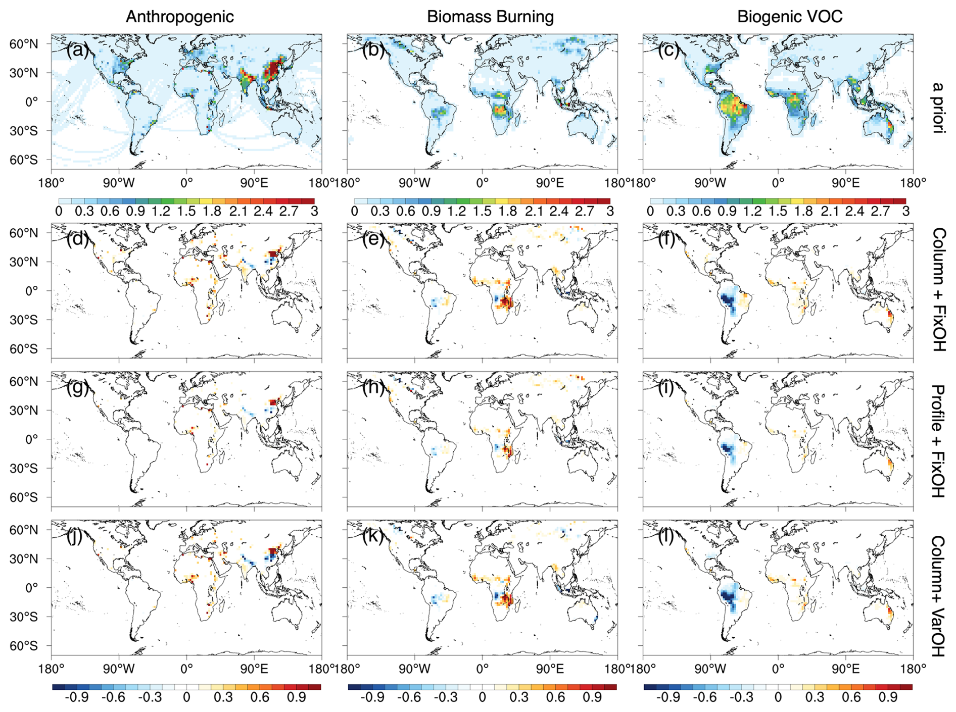
Figure 1 Spatial patterns of a priori CO sources and a posteriori scaling factors for the period 2003–2022. (a–c) Mean a priori CO sources (10¹² $\mathrm{molec}.{\mathrm{cm}}^{-\mathrm{2}}{\mathrm{s}}^{-\mathrm{1}}$). (d–l) Scaling factors (ratio of a posteriori to a priori sources) derived from the three inversion experiments: (d–f) Column-FixOH, (g–i) Profile-FixOH, and (j–l) Column-VarOH.

The global default anthropogenic emission inventory is the CEDS-CMIP6 (Community Emissions Data System) (Hoesly et al., 2018). Regional emissions are replaced as follows: MIX (Li et al., 2017) over Asia, NEI 2016 (National Emissions Inventory) over the United States, DICE_AFRICA and EDGARv4.3 over Africa, and APEI over Canada. The contribution of co-emitted anthropogenic VOC sources is considered by scaling up anthropogenic CO emissions by 11 %. Biogenic sources are simulated using the Model of Emissions of Gases and Aerosols from Nature, version 2.0 (MEGANv2.0, Guenther et al., 2006). CH₄ oxidation source is considered by using a prescribed, spatially varying CH₄ field following the default tagged-CO configuration (Fisher et al., 2017). The CO sources from both biogenic VOCs and CH₄ oxidation are calculated online based on the assumption of instantaneous oxidation by OH radicals. Biomass burning emissions are based on the Global Fire Emissions Database version 4 (GFED4, van der Werf et al., 2010). For years beyond the end year of a specific inventory, emissions from the last available year within that inventory's coverage were used to fill the subsequent years. The distribution of the annual mean CO emissions from 2003 to 2022 is shown in Fig. 1a–c.

The annual global sources are 536.3 Tg yr⁻¹ from anthropogenic emissions, 312.5 Tg yr⁻¹ from biomass burning, 623.2 Tg yr⁻¹ from the oxidation of biogenic VOCs, 922.5 Tg yr⁻¹ from the oxidation of CH₄, with a total sink (through the reaction with OH radicals) of approximately 2395.0 Tg yr⁻¹ in a priori inventories in this work. For comparison, Zheng et al. (2019) reported inversion-based global CO budget estimates for 2005–2017 of approximately 700 Tg yr⁻¹ for anthropogenic emissions, 500 Tg yr⁻¹ for biomass burning, 300 Tg yr⁻¹ for biogenic VOC oxidation, and 900 Tg yr⁻¹ for CH₄ oxidation, with a total sink of approximately 2600 Tg yr⁻¹. Regarding anthropogenic emissions, the CEDS-CMIP6 inventory estimates an average of 607.6 Tg yr⁻¹ for 2003–2014, while the updated CEDS-CMIP7 inventory yields lower values, averaging 480.2 Tg yr⁻¹ over 2003–2023. For biomass burning, the GFED5 inventory estimates an average of 518.3 Tg yr⁻¹ for 2003–2022.

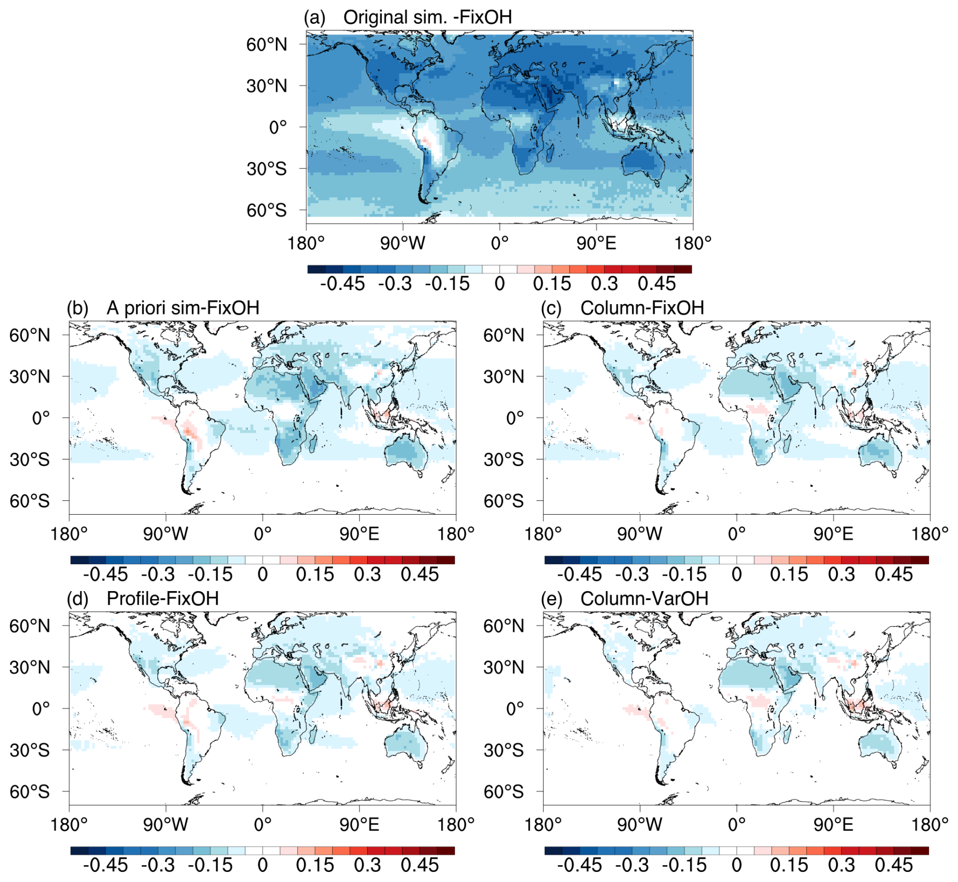
Figure 2 Relative bias in column CO for 2003–2022, calculated as $(\text{Model}-\text{MOPITT})/\text{MOPITT}$ for GC-original (a), GC-a priori (b), and a posteriori simulations (c–e).

The objective of the 4D-Var approach is to minimize the difference between simulations and observations by minimizing the cost function (Henze et al., 2007):

$$\begin{array}{}\text{(1)}& \begin{array}{rl}J\left(\mathit{x}\right)& ={\sum }_{i=\mathrm{1}}^N\left({\mathbf{F}}_i\right(\mathit{x})-{\mathit{z}}_i{)}^T{\mathbf{S}}_{\mathrm{\Sigma }}^{-\mathrm{1}}({\mathbf{F}}_i\left(\mathit{x}\right)-{\mathit{z}}_i)\\ & +\mathit{\gamma }(\mathit{x}-{\mathit{x}}_a{)}^T{\mathbf{S}}_a^{-\mathrm{1}}(\mathit{x}-{\mathit{x}}_a)\end{array}\end{array}$$

where x is the state vector of CO emissions, N is the number of observations distributed in time over the assimilation period, z_i are the MOPITT CO retrievals, and F(x) is the forward model. Error estimates are assumed to be Gaussian: S_Σ is the observational error covariance, which combines a 10 % uniform error and the MOPITT CO retrieval error covariance; and S_a is a priori error covariance. Here the combustion-related CO sources (fossil fuel, biofuel, and biomass burning) and the oxidation source from biogenic VOCs are combined, with a uniform a priori error of 50 % assumed following previous studies (Jiang et al., 2013, 2017). The CO source from CH₄ oxidation is optimized separately as an aggregated global source, with a priori uncertainty of 25 %. The cost function is minimized by iteratively adjusting the CO emissions using the quasi-Newton gradient-based optimization L-BFGS-B algorithm (Zhu et al., 1997) and the adjoint gradients:

$$\begin{array}{}\text{(2)}& \begin{array}{rl}{\mathrm{\nabla }}_{\mathit{x}}J\left(\mathit{x}\right)& ={\sum }_{k=\mathrm{1}}^N\left[\mathrm{2}{\left({\displaystyle \frac{\partial {\mathit{F}}_i}{\partial \mathit{x}}}\right)}^{\mathit{T}}{\mathit{S}}_{\mathrm{\Sigma }}^{-\mathrm{1}}\left({\mathit{F}}_i\right(\mathit{x})-{\mathit{z}}_i)\right]\\ & +\mathrm{2}\mathit{\gamma }(\mathit{x}-{\mathit{x}}_a{)}^T{\mathit{S}}_a^{-\mathrm{1}}.\end{array}\end{array}$$

The LOGX2 method (Jiang et al., 2015a, 2017) is employed to improve the reduction of negative gradients.

Table 1 Mean biases of modeled CO concentrations relative to satellite (MOPITT) and in-situ (WDCGG, HIPPO, ATom) observations for five model simulations over the period 2003–2022. Biases are in units of 10¹⁶ $\mathrm{molec}.{\mathrm{cm}}^{-\mathrm{2}}$ for MOPITT and ppb for other datasets.

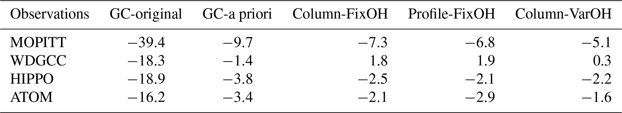
Following Jiang et al. (2017), we applied a two-step approach to mitigate the influence of systematic biases in the model simulations. First, a sequential Kalman filter (Todling and Cohn, 1994; Tang et al., 2022) was used to assimilate MOPITT CO retrievals from 1 October 2002 to 31 December 2022, providing optimized CO concentration fields with lower bias. As illustrated in Fig. 2a, the GEOS-Chem model driven by the original monthly CO initial conditions and a priori emission inventories (referred to as GC-original) substantially underestimated column CO concentrations by approximately 30 %–40 % ($\text{mean bias}=-\mathrm{39.4}\times {\mathrm{10}}^{\mathrm{16}}$ $\mathrm{molec}.{\mathrm{cm}}^{-\mathrm{2}}$; Table 1). In contrast, simulations using the monthly CO initial conditions derived from the sequential Kalman filter together with a priori emissions (GC-a priori) showed markedly improved agreement with MOPITT CO retrievals (Fig. 2b), reducing the mean bias to about 10 % ($\text{mean bias}=-\mathrm{9.7}\times {\mathrm{10}}^{\mathrm{16}}$ $\mathrm{molec}.{\mathrm{cm}}^{-\mathrm{2}}$). Similarly, the use of optimized monthly CO initial conditions led to considerable improvement in model performance against independent surface and aircraft measurements (Table 1). The mean bias decreased from −18.3 ppb (GC-original) to −1.4 ppb (GC-a priori) for World Data Centre for Greenhouse Gases (WDCGG) surface observations; from −18.9 to −3.8 ppb for HIAPER Pole-to-Pole Observations (HIPPO) aircraft data; and from −16.2 to −3.4 ppb for Atmospheric Tomography Mission (ATom) aircraft measurements. These results suggest that the substantial negative biases seen in Fig. 2a largely originate from the accumulation of biases over preceding months.

Furthermore, ocean scenes (pink grids in Fig. S3) were defined as land boundary conditions. The optimized CO fields from the Kalman filter were used to update CO concentrations over the ocean at hourly intervals during the forward simulation within the 4D-Var process. Meanwhile, the 4D-Var system constrained CO emissions over land without modifying oceanic CO distributions. As demonstrated by Jiang et al. (2017), the use of optimized CO land boundary conditions in 4D-Var assimilation effectively reduces systematic biases associated with long-range transport. By adopting this two-step assimilation framework, the inversion focuses on optimizing fresh continental CO emissions, while reducing the influence of uncertainties arising from transport and chemical processes, which tend to exhibit larger systematic biases. Consequently, a posteriori CO emissions estimated in this study are expected to be lower than those derived without adjustments to the initial and boundary CO conditions. This reflects both the specific inverse modeling setup and a possible underestimation in our a posteriori emission estimates, attributable to the emphasis on constraining fresh continental CO sources.

Based on this assimilation framework, three sets of CO emission inversion experiments are designed:

1. Column-FixOH: uses MOPITT CO column concentration data with default OH fields fixed in 2013.

2. Profile-FixOH: uses MOPITT CO profile data with default OH fields fixed in 2013.

3. Column-VarOH: uses MOPITT CO column concentration data with variable OH fields from the TCR-2 tropospheric chemistry reanalysis.

By comparing the results of Column-FixOH and Profile-FixOH, the influence of different MOPITT CO data types on CO source estimates can be assessed. Similarly, comparing Column-FixOH and Column-VarOH allows for evaluation of the impact of different OH fields on CO source estimates.

2.2 MOPITT CO retrievals

The MOPITT instrument was launched on 18 December 1999, aboard the NASA Terra spacecraft. The satellite follows a sun-synchronous polar orbit at 705 km altitude, crossing the equator at 10:30 LT. The instrument made measurements over a 612 km cross-track scan, with a footprint of 22 km×22 km. The MOPITT data used in this study are from the joint retrieval (version 9J) of CO, which combines thermal infrared (TIR, 4.7 µm) and near-infrared (NIR, 2.3 µm) radiances using an optimal estimation approach (Worden et al., 2010; Deeter et al., 2022). The retrieved volume mixing ratios are reported as layer averages across 10 pressure levels (surface, 900, 800, 700, 600, 500, 400, 300, 200, and 100 hPa). The relationship between the retrieved CO profile and the true atmospheric state is expressed as:

$$\begin{array}{}\text{(3)}& \widehat{\mathit{z}}={\mathit{z}}_a+\mathbf{A}(\mathit{z}-{\mathit{z}}_a)+\mathbf{G}\mathit{ϵ}\end{array}$$

where z_a is the MOPITT a priori CO profile, z is the true atmospheric state, Gε represents the retrieval error, and $\mathbf{A}=\partial \widehat{\mathit{z}}/\partial \mathit{z}$ is the MOPITT averaging kernel matrix, indicating the sensitivity of the retrieval to the actual atmospheric CO. We only consider data with Cloud Description=2 (cloud free) and exclude MOPITT data with CO column amounts less than 5×10¹⁷ $\mathrm{molec}.{\mathrm{cm}}^{-\mathrm{2}}$. The threshold (5×10¹⁷ $\mathrm{molec}.{\mathrm{cm}}^{-\mathrm{2}}$) was selected to prevent the influence of certain potentially inaccurate, extremely low-concentration observations, which may also have low observation errors in the cost function, on the 4D-Var assimilation (Jiang et al., 2013, 2017). Since the NIR channel relies on reflected solar radiation, only daytime data are considered (Worden et al., 2010; Tang et al., 2024).

2.3 Aircraft and surface CO measurements

The HIPPO (Wofsy and HIPPO Science Team, 2011) were conducted using the Gulfstream V aircraft from 2009 to 2011. The flights primarily covered the Pacific Ocean, spanning latitudes from 67° S to 87° N, with continuous sampling from 0.2 to 12 km altitude. The ATom (Wofsy and Atom Science Team, 2018) used the DC-8 aircraft from 2016 to 2018. ATom covered similar altitude and latitudinal ranges as HIPPO but with broader spatial coverage, particularly over the Atlantic Ocean. For HIPPO, a total of 687 CO profiles from five missions were used directly. For ATom, CO measurements during continuous ascents and descents were used to construct 523 CO profiles from four missions. Surface CO measurements from the WDCGG are also included in this analysis. The WDCGG, operated by the Japan Meteorological Agency under the World Meteorological Organization's Global Atmosphere Watch (GAW) program, collects, archives, and distributes atmospheric greenhouse gas data, including CO, contributed by various institutions worldwide.

3 Results and discussion

3.1 Evaluation of assimilation system performance

Before presenting the estimated emission trends, we first evaluate the performance of our assimilation system. The evaluation involves comparing modeled CO concentrations from the GC-original, GC-a priori, and a posteriori simulations (Column-FixOH, Profile-FixOH, Column-VarOH) over the period 2003–2022 against MOPITT satellite measurements, as well as independent surface observations from WDCGG and aircraft measurements from HIPPO and ATom. As summarized in Table 1, a posteriori simulations exhibit mean biases relative to MOPITT retrievals ranging from −5.1 to $-\mathrm{7.3}\times {\mathrm{10}}^{\mathrm{16}}$ $\mathrm{molec}.{\mathrm{cm}}^{-\mathrm{2}}$. These values are notably smaller than the biases in the GC-a priori simulation ($-\mathrm{9.7}\times {\mathrm{10}}^{\mathrm{16}}$ $\mathrm{molec}.{\mathrm{cm}}^{-\mathrm{2}}$) and the GC-original simulation ($-\mathrm{39.4}\times {\mathrm{10}}^{\mathrm{16}}$ $\mathrm{molec}.{\mathrm{cm}}^{-\mathrm{2}}$). Similarly, for the HIPPO aircraft observations, a posteriori simulations show mean biases between −2.5 and −2.1 ppb, improved compared to the GC-a priori (−3.8 ppb) and GC-original (−18.9 ppb) simulations. For ATom aircraft data, a posteriori mean biases range from −2.9 to −1.6 ppb, also lower than those from the GC-a priori (−3.4 ppb) and GC-original (−16.2 ppb) simulations. In the case of surface CO concentrations, a posteriori simulations yield mean biases between 0.3 and 1.9 ppb relative to WDCGG observations (Table 1), which are reduced compared to GC-original (−18.3 ppb) simulations, and comparable with the GC-a priori (−1.4 ppb) simulations. A posteriori simulations slightly overestimate surface concentrations relative to WDCGG data, while underestimating CO in the free troposphere according to MOPITT and aircraft measurements. This systematic discrepancy may be attributable to uncertainties in convective transport parameterizations within the model.

Overall, the good consistency between a posteriori simulations and multiple independent observation platforms demonstrates the capability of our assimilation system to effectively constrain CO emissions. Given this confidence in the system's performance, we now present the central findings of this study: the long-term evolution of CO emissions. As mentioned in Sect. 2.1, the combustion-related CO sources and the oxidation source from biogenic VOCs are combined, and thus, the inverse system optimizes total CO emissions within each model grid cell. The subsequent attribution of emissions to specific source types (e.g., anthropogenic, biomass burning) in an individual grid cell is based on the relative contribution of each source category from a priori emission inventories. Specifically, a posteriori emission for a given source type in a grid cell is calculated by applying the grid-scale scaling factor (the ratio of a posteriori to a priori total emissions) to the corresponding a priori emission of that source type. Different sources can finally be calculated because each source category possesses distinct spatial patterns and seasonal variations.

3.2 Long-term evolution of global CO emissions

3.2.1 Anthropogenic CO emissions

At the global scale, anthropogenic CO emissions based on three inversion configurations are estimated to be 7 %–14 % higher than a priori values (Table 2) in 2003–2022 and show a clear declining trend (Fig. 3f). Under the Column-FixOH configuration, global anthropogenic emissions from 2003 to 2022 ranged from 546.1 to 654.1 Tg yr⁻¹, with a multi-year average of approximately 610 Tg yr⁻¹ and a total reduction of about 17 %; similar emission ranges and reduction rates (14 %–17 %) were obtained under the Profile-FixOH and Column-VarOH configurations. These results are broadly consistent with Zheng et al. (2019). The CEDS-CMIP7 inventory (Hoesly et al., 2018) shows significantly lower global CO emissions than those derived from inverse modeling, though its decreasing trend is comparable. As shown in Fig. 4a, negative trends (blue) were concentrated in three major industrialized regions: eastern North America, Europe, and eastern China, forming a “reduction belt”. These regions accounted for over 65 % of global anthropogenic CO emissions, and their systematic reductions constituted the principal driver of the global downward trend. In contrast, positive trends (red) were primarily distributed in northern India (increases of 15.2 %–22.3 %) and Central Africa, corresponding to rapid urbanization and industrialization processes.

Table 2 Mean anthropogenic CO emissions (Tg yr⁻¹) and their trends (Tg yr⁻²) in 2003–2022: A comparison of a priori inventories with those constrained by MOPITT retrievals under different configurations. The region definition is shown in Fig. S1e in the Supplement.

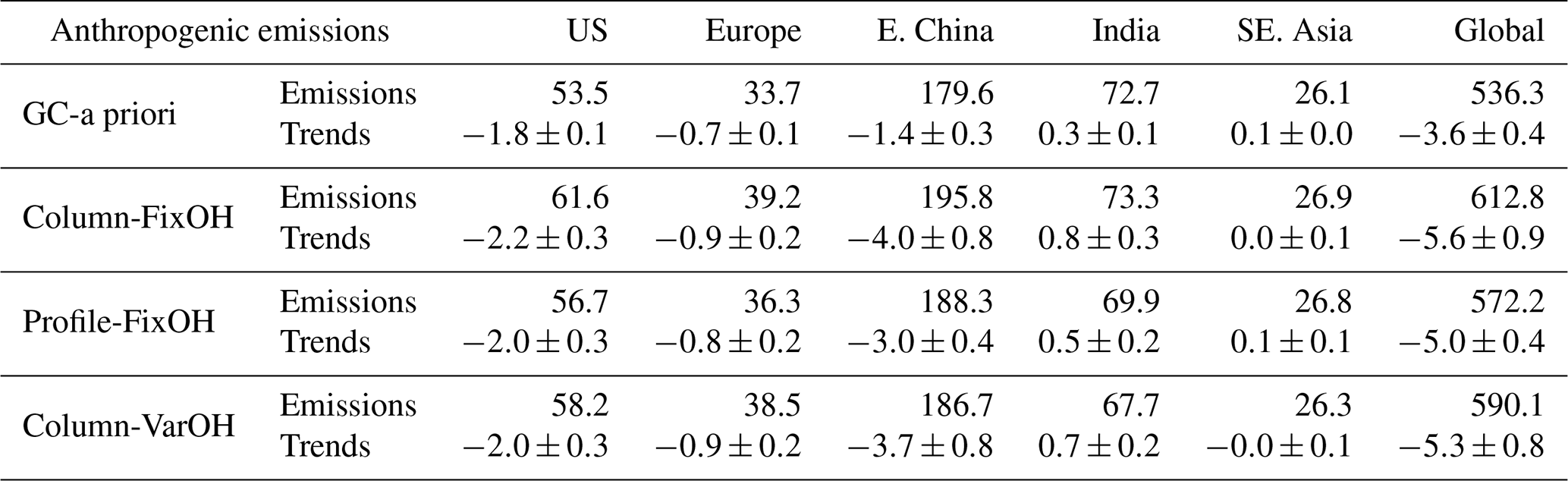
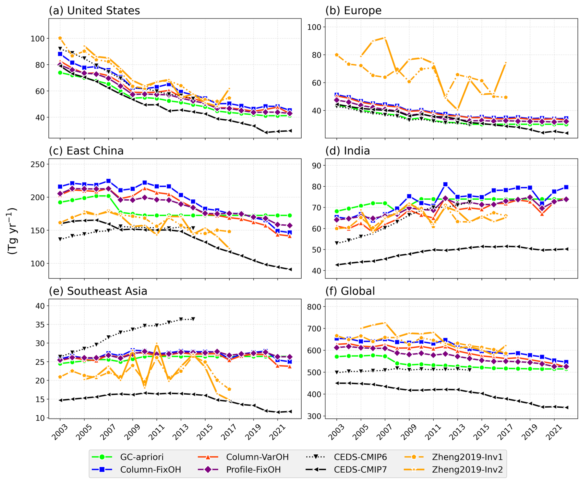
Figure 3 Time series of anthropogenic CO emissions from 2003 to 2022 across major regions, comparing a priori inventories, a posteriori inversions from this study, and independent estimates from CEDS-CMIP6/7 and Zheng et al. (2019).

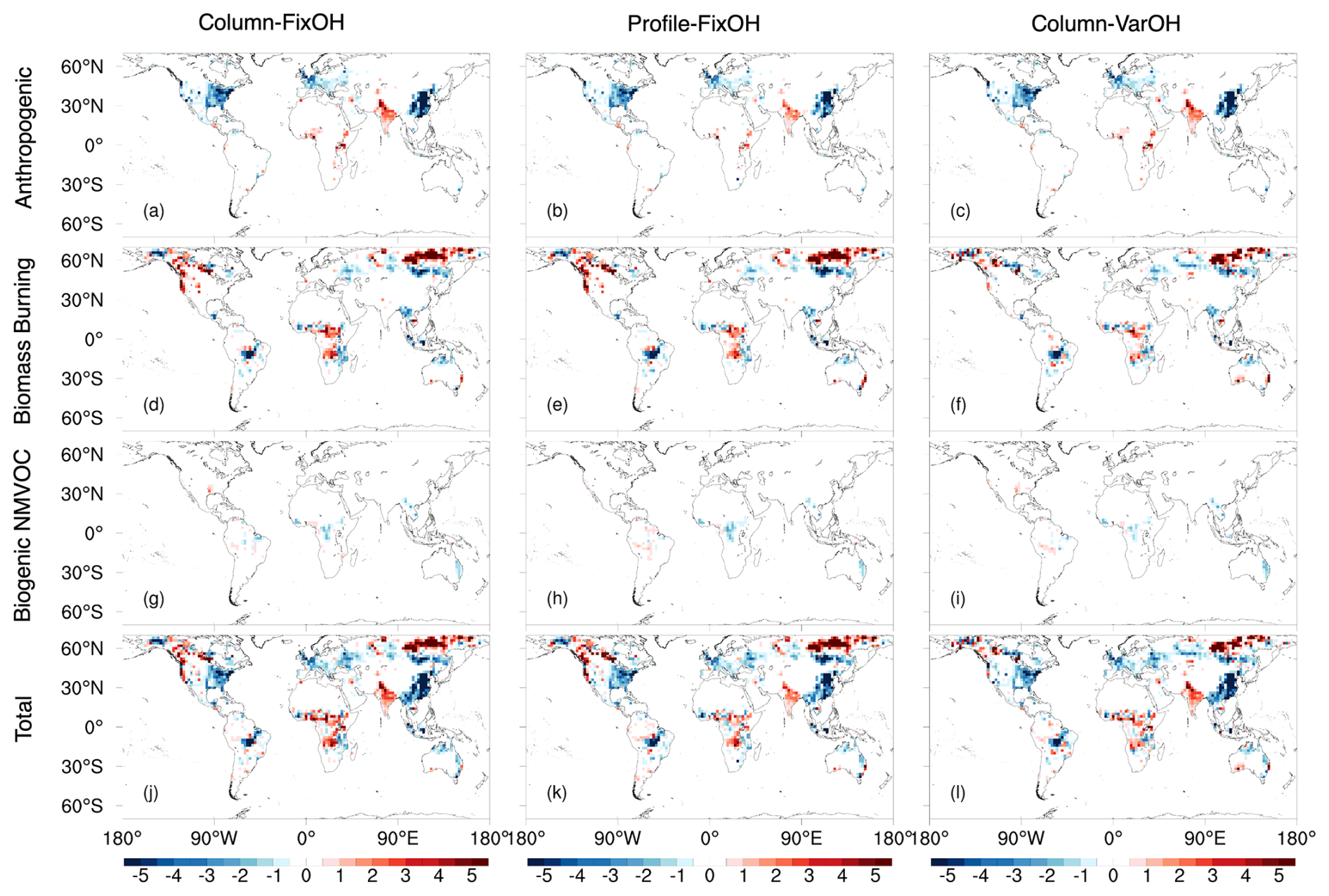
Figure 4 Long-term trends in CO sources (10¹⁰ $\mathrm{molec}.{\mathrm{cm}}^{-\mathrm{2}}{\mathrm{s}}^{-\mathrm{1}}{\mathrm{yr}}^{-\mathrm{1}}$) as constrained by the three inversion experiments (2003–2022). For anthropogenic and biogenic VOC trends, months dominated by biomass burning (>50 % contribution) were excluded in this figure. This approach ensures that the derived trends more accurately reflect the actual changes in anthropogenic and biogenic VOC sources, without being biased by short-term, seasonal biomass burning signals.

In the United States (US), emissions declined rapidly from 2003 to 2009, followed by a period of slower reduction (Fig. 3a). Over the entire period (2003–2022), US CO emissions decreased at rates of 2.0–2.2 Tg yr⁻¹, resulting in a cumulative reduction of 46 %–49 % (Table S1 in the Supplement). This phased reduction pattern is consistent with the diminishing marginal effects of widespread transportation control technologies, as supported by independent studies (Elguindi et al., 2020; Miyazaki et al., 2020). Our estimated emission magnitude and decreasing trend are similar to Zheng et al. (2019) and the CEDS-CMIP7 in the US. European CO emissions (Fig. 3b) followed a similar pattern (cumulative reduction of 32 %–34 % over 2003–2022). Estimated emissions over Europe in Zheng et al. (2019) are substantially higher than ours and show stronger interannual variability. In comparison, the CEDS-CMIP7 inventory shows good agreement with our results during 2003–2017, but a faster decline after 2017; and Fortems-Cheiney et al. (2024) suggests continuous decline in CO emissions in Europe in 2011–2021. This discrepancy could be possibly attributable to differences in the processing of initial and boundary CO conditions (e.g., the use of climatological CO concentrations in Fortems-Cheiney et al., 2024).

The evolution of eastern China's CO emissions can be divided into four stages (Fig. 3c): (1) a slight growth until 2007, peaking around that time; (2) a sharp decline of approximately 7 % during the 2008 global financial crisis; (3) a temporary rebound from 2008 to 2010 under economic stimulus policies; and (4) a continuous decline phase after 2010. From 2003 to 2022, anthropogenic CO emissions from eastern China decreased at an average rate of 3.0–4.0 Tg yr⁻¹ (Table 2), with a cumulative reduction of 23 %–32 % (Table S1). Zhao et al. (2012) and Xia et al. (2016) confirmed the trend reversal around 2007, attributing it to improved energy efficiency and strengthened emission controls, while Lin and McElroy (2011) and Tong et al. (2016) highlighted the suppressive impact of the 2008 economic recession. Both Zheng et al. (2019) and the CEDS-CMIP7 emission dataset show a declining trend consistent with our results, although their emission magnitudes are lower. During 2019–2022, the emission reduction rate accelerated to 4.8–8.3 Tg yr⁻¹, reflecting not only the short-term impact of the COVID-19 pandemic but also the long-term cumulative effects of clean air policies and energy structure transformation.

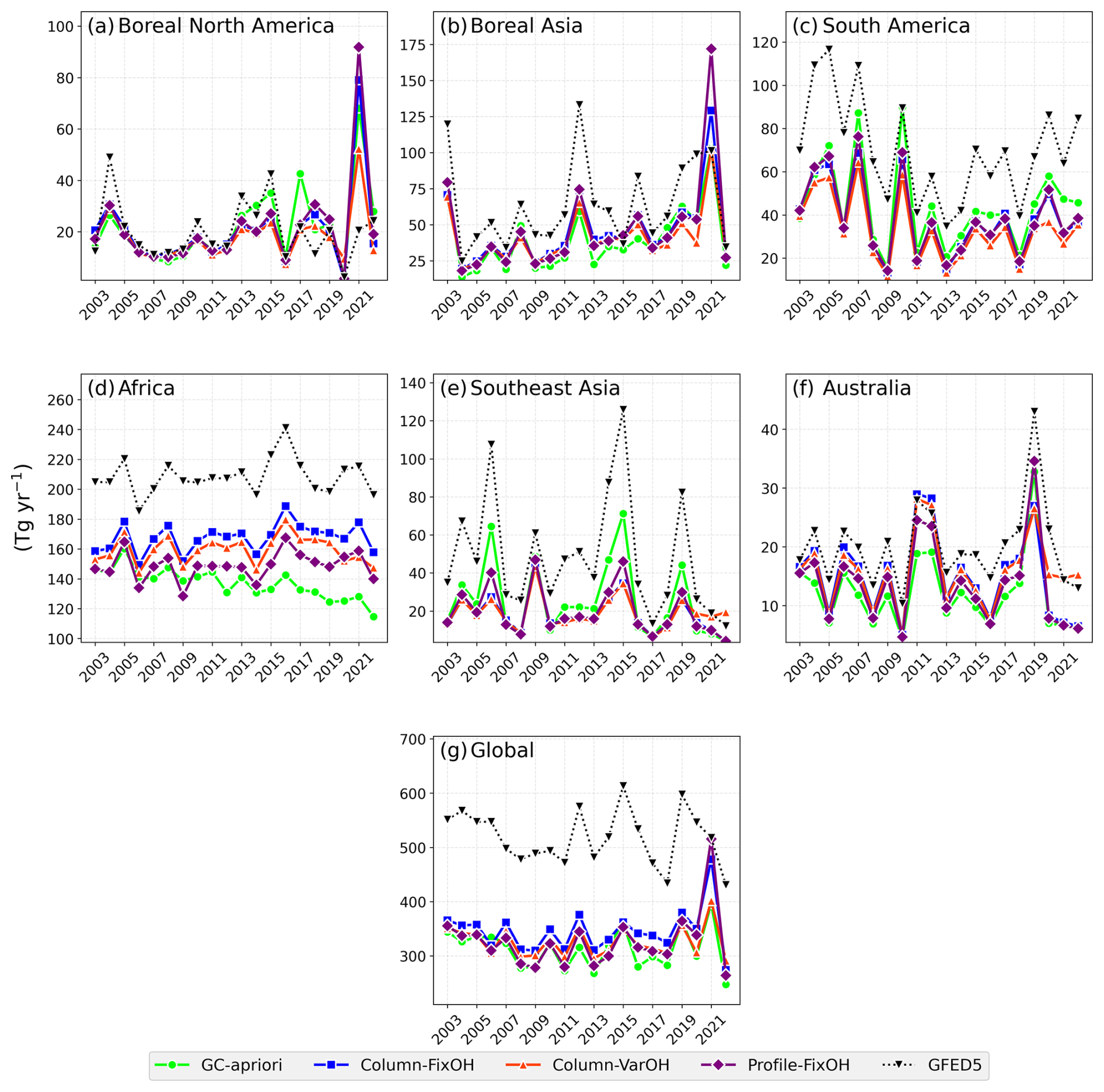
Figure 5 Time series of biomass burning CO emissions from 2003 to 2022, comparing the a priori inventory (GFED4), a posteriori inversions, and the GFED5 inventory.

India exhibited a continuous growth in anthropogenic CO emissions from 2003 to 2009, followed by a period of slower increase, with an average annual increase of 0.5–0.8 Tg yr⁻¹ in 2003–2022. Our estimated emission magnitude and trend are similar to Zheng et al. (2019) in India. In comparison, the CEDS-CMIP7 inventory shows a similar trend, but its emission levels are lower than those derived from inverse modeling. In Southeast Asia, anthropogenic CO emissions exhibited a relatively stable and slow upward trend over the study period, though a noticeable decline occurred from 2019 to 2022, which is likely associated with the impact of the COVID-19 pandemic. The emission trend derived from our inversion is generally consistent with that reported by Zheng et al. (2019) for this region, although their estimates show stronger interannual variability. Compared with the CEDS-CMIP7 inventory, the trend in CO emissions is similar to our results, but the emission magnitude in CEDS-CMIP7 is lower than that derived from inverse modeling.

3.2.2 Biomass burning CO emissions

Globally, biomass burning CO emissions were 4 %–11 % higher than a priori estimate in 2003–2022 (Table 3) and reached a historical peak of approximately 500 Tg yr⁻¹ in 2021 (Fig. 5g). In contrast to the clear decline of anthropogenic emissions, the trend in global biomass burning CO emissions remains insignificant (Table 3). A comparison with the GFED5 emission inventory (van der Werf et al., 2025) reveals noticeable differences: GFED5 estimates are generally higher than our results (Fig. 5g), and do not show the 2021 peak. Spatial analysis revealed a pronounced latitudinal differentiation in the changes of biomass burning CO emissions (Fig. 4d–f): positive trends (red) were concentrated in Northern Hemisphere high-latitude coniferous forests, while negative trends (blue) dominated tropical and subtropical regions. This pattern is consistent with the “global fire emission geographic reconstruction” observed by Zheng et al. (2023), reflecting the differential impacts of climate change across latitudinal zones.

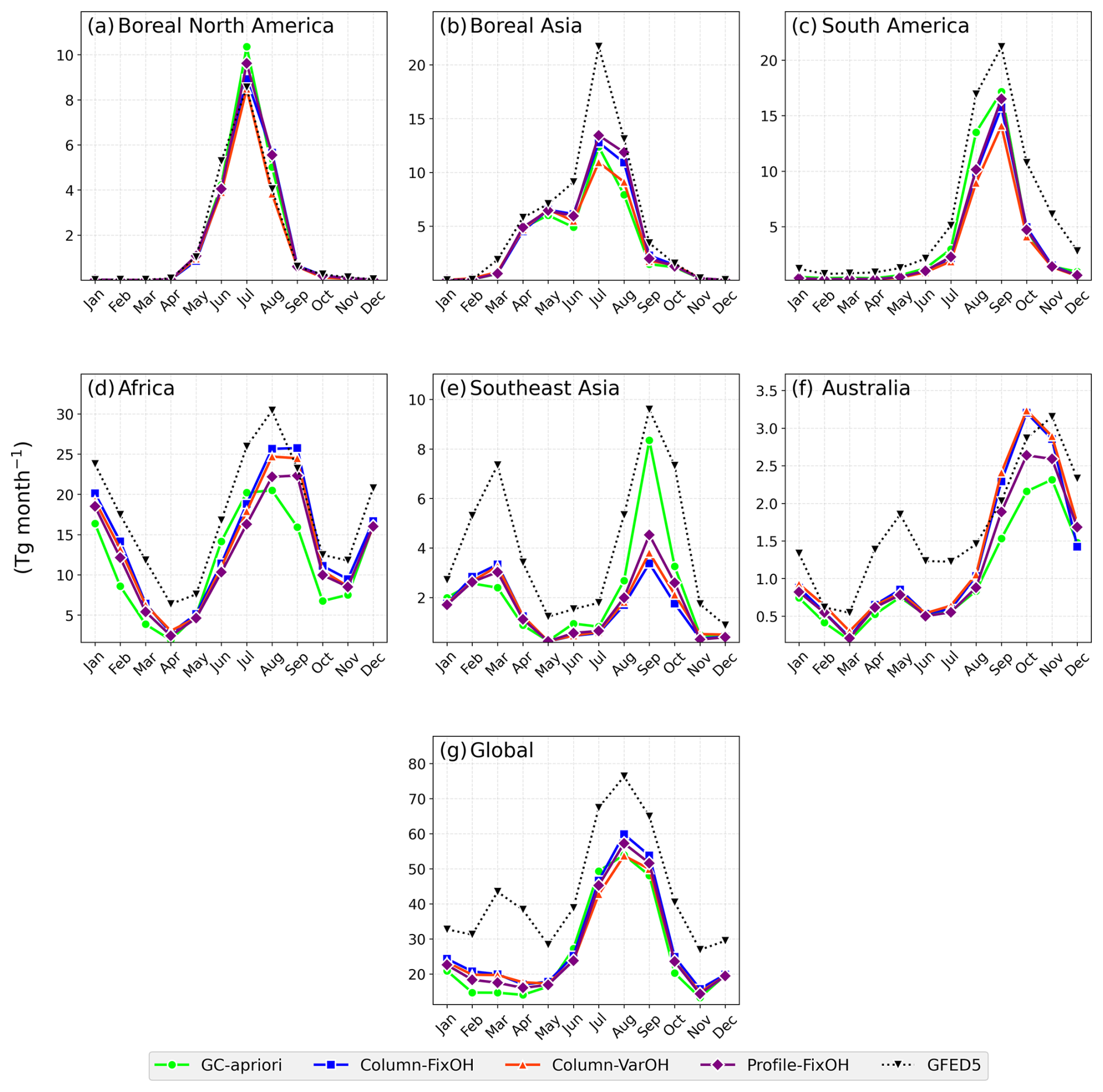
Figure 6 Climatological monthly cycle (2003–2022 average) of biomass burning CO emissions across different regions, comparing a priori (GFED4) and a posteriori estimates with GFED5.

Table 3 Mean biomass burning CO emissions (Tg yr⁻¹) and their trends (Tg yr⁻²) in 2003–2022: A comparison of a priori inventories (GFED4) with those constrained by MOPITT retrievals under different configurations. The region definition is shown in Fig. S1f.

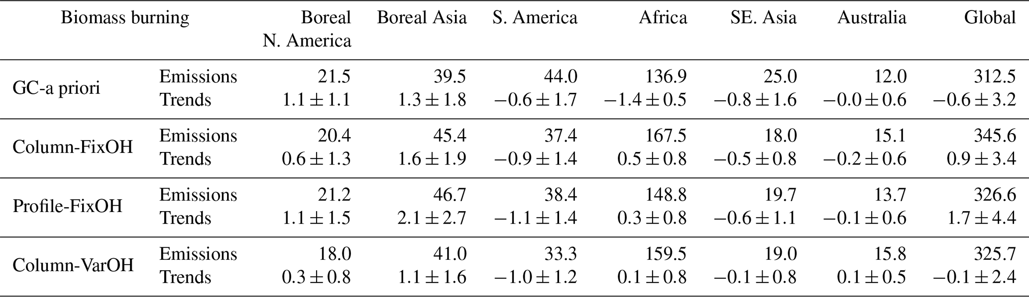
Emissions from high-latitude coniferous forests have shown different long-term trends between boreal North America and boreal Asia over the past two decades (Fig. 5a and b). Peak fire activity in boreal North America occurs during June–August (Fig. 6a); boreal Asia experiences its primary fire season in June–August, with a secondary peak often observed in March–May (Fig. 6b). When excluding the exceptional wildfire year of 2021, summertime biomass burning CO emissions in boreal North America exhibited an overall declining trend from 2003 to 2022 (Fig. 7a). In contrast, boreal Asia experienced a general increase in summertime biomass burning CO emissions during the same period, even when 2021 is omitted, though the trend is less pronounced than when including that extreme year (Fig. 7b). The peak in wildfire emissions from high-latitude coniferous forests in 2021 was triggered by severe, concurrent droughts across the Northern Hemisphere (Zheng et al., 2023). The pronounced latitudinal amplification of emissions is consistent with higher carbon emission density of boreal forests, which is 4–10 times greater than that of grasslands (Zheng et al., 2021). GFED5 data suggests that boreal Asia's wildfire emissions peaked in 2012, different from emission inversion results in this work and Zheng et al. (2023).

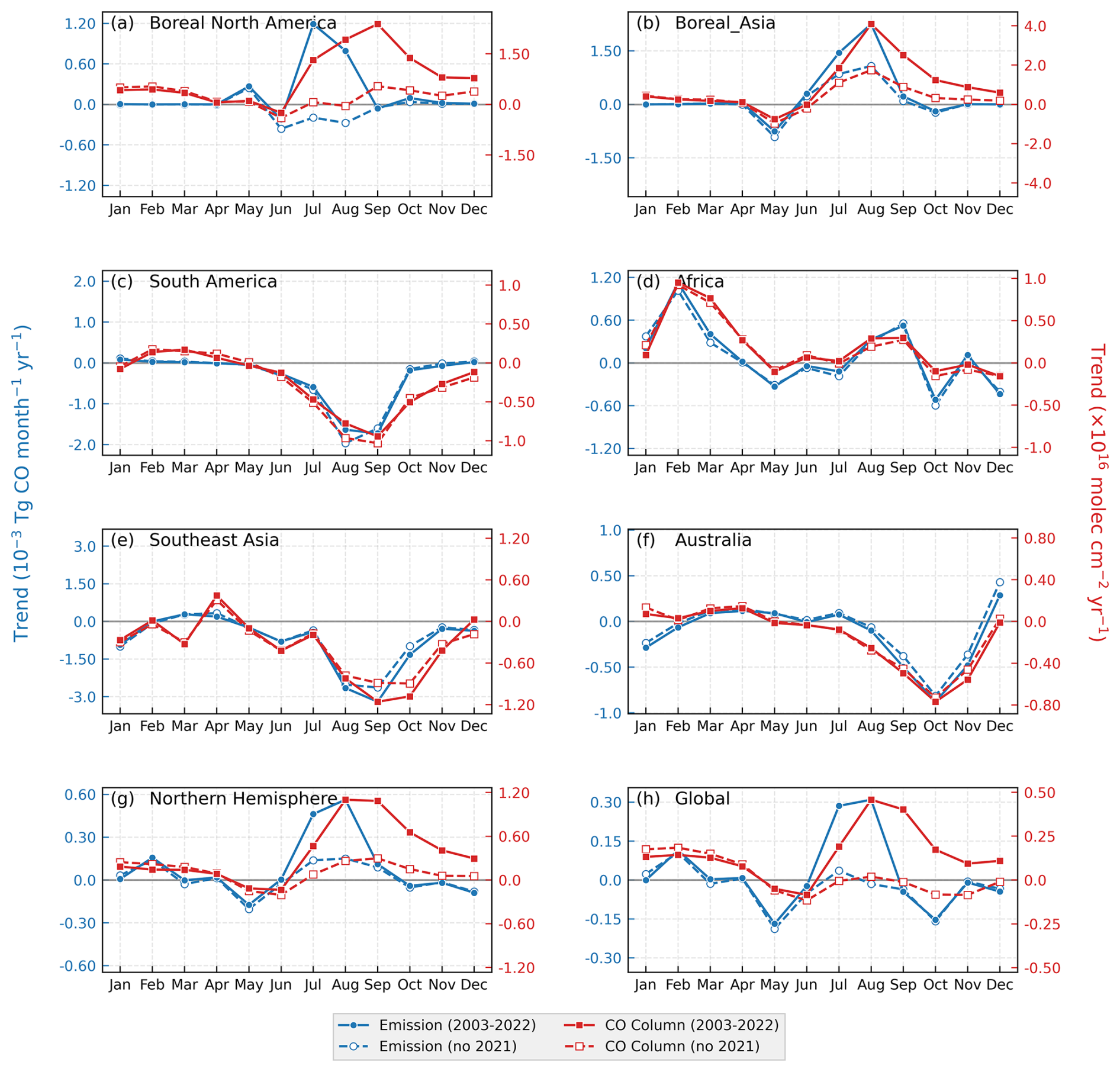
Figure 7 Monthly trends in biomass burning CO emissions (based on Column-FixOH) and their impact on column CO concentrations (2003–2022). Solid lines show trends including 2021, while dashed lines exclude 2021 to illustrate the impact of extreme fire year. Please check Figs. S4 and S5 for the standard deviation of the trends.

A notable decline in fire activity in South America occurred after 2010 (Fig. 5c), particularly in August–September (Fig. 7c) coinciding with the peak wildfire season in South America (Fig. 6c). The trend shift in CO emissions are consistent with the sharp reductions in annual deforestation rates in the Brazilian Amazon from 25 396 km² yr⁻¹ in 2003 to 7000 km² yr⁻¹ in 2010 (Deeter et al., 2018). Africa experiences its primary fire season in June–September, with a secondary peak often observed in December–February (Fig. 6d). Biomass burning CO emissions in Africa exhibited a modest increasing trend overall (Fig. 5d), particularly in February (Fig. 7c). Pronounced regional differentiation occurred, with increases in central Africa and decreases in surrounding areas (Fig. 4d–f), reflecting the “strong contrast” pattern described by Andela et al. (2017). Compared to the GFED5 inventory, our inversion results generally show lower CO emission intensities.

Peak fire activity in Australia occurs during August–December (Fig. 6f); Southeast Asia experiences its primary fire season in August–October, with a secondary peak often observed in February–March (Fig. 6e). Emission patterns in Southeast Asia (Fig. 5e) and Australia (Fig. 5f) highlighted their sensitivity to large-scale climate oscillations. Major fire events in Indonesia in 2006, 2009, 2015, and 2019 were closely linked to El Niño-induced droughts (Page et al., 2009; Field et al., 2016). Australia's extreme fires in 2019 resulted from compound extreme climate conditions influenced by the El Niño-Southern Oscillation, the Southern Annular Mode, and the Indian Ocean Dipole (Deb et al., 2020). Building upon the observed sensitivity to large-scale climate oscillations, the long-term interannual trend of wildfire emissions across Southeast Asia and Australia remains insignificant, despite decline in August–October in Southeast Asia (Fig. 7e) and September–November in Australia (Fig. 7f). Our emission inversion shows lower CO emissions than GFED5 inventory in Southeast Asia and Australia.

3.2.3 Difference between combustion and biogenic NMVOC sources

CO from combustion sources in the Northern Hemisphere showed strong regional differentiation (Fig. 4), reflecting a dynamic redistribution between declining anthropogenic sources and increasing biomass burning sources. Positive trends were densely distributed in high-latitude regions, mainly due to increases in wildfires; Negative trends dominated mid-to-low latitude industrialized areas. Tropical regions showed a mixed pattern, while the Southern Hemisphere exhibited generally weaker trends. This spatial heterogeneity confirms a net global decrease in combustion-related CO, revealing a clear contrast between increases at high northern latitudes and decreases at mid-latitudes, reflecting the compound influences of industrialization, policy interventions and climate change.

In contrast, CO produced from the oxidation of biogenic VOCs remained relatively stable from 2003 to 2022 (Fig. 4g–i). This stability aligns with findings by Messina et al. (2016), suggesting that global-scale biogenic VOC sources are less sensitive to short-term climate and land cover changes. The global stability of biogenic VOC-derived CO is important for atmospheric chemistry, as these compounds are key reactants for OH radicals and play a regulatory role in atmospheric oxidation capacity. This stable background provides a crucial baseline for understanding changes in atmospheric oxidation processes. The weaker trends compared to those reported by Jiang et al. (2017) may be associated with our use of continuous MERRA-2 meteorological data, which enhances consistency in long-term analysis.

3.3 Long-term evolution and drivers of global CO concentrations

Building on the emission estimates evaluated above, this section investigates their ultimate influence in the atmosphere by analyzing the spatiotemporal patterns and trends of CO concentrations. We first present the mean state and long-term changes in CO concentrations, and then quantitatively attribute these changes to their underlying drivers: emissions and meteorology. Figure 8a–c show the mean surface CO concentrations in 2003–2022 from a posteriori simulations and WDCGG surface observations. Higher CO concentrations are evident in regions with strong anthropogenic emissions, such as East Asia, India, and Southeast Asia, as well as in areas with significant biomass burning, i.e., Central Africa and South America. The long-term trends in surface CO (Fig. 8d–f) reveal declining concentrations over North America, Europe, East Asia, and South America, which contrast with rising trends over India, Boreal Asia, Central Africa, and Australia. The 20 year mean CO columns (Fig. 9a–c) show a consistent spatial pattern, with the highest column concentrations over East Asia and Central Africa, followed by South America, India, and Southeast Asia. In contrast, the long-term trend of CO columns (Fig. 9d–f) exhibits a more uniform decrease across the Northern Hemisphere, lacking the distinct regional hotspots observed in the surface trends. This suggests that changes in CO are more thoroughly mixed within the column.

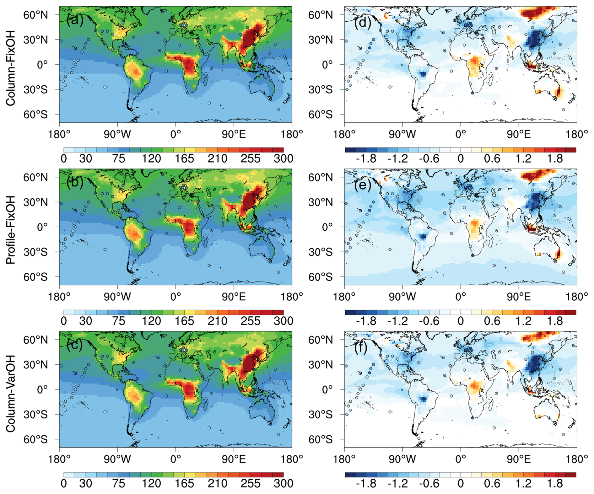
Figure 8 Modeled surface CO concentrations (ppb) and their trends (% yr⁻¹) from 2003 to 2022. (a–c) Mean concentrations from WDCGG observations and model simulations. (d–f) Spatial pattern of the long-term trend. Only stations with 14 year observations (the time range between the first and last observations) during 2003–2022 are included.

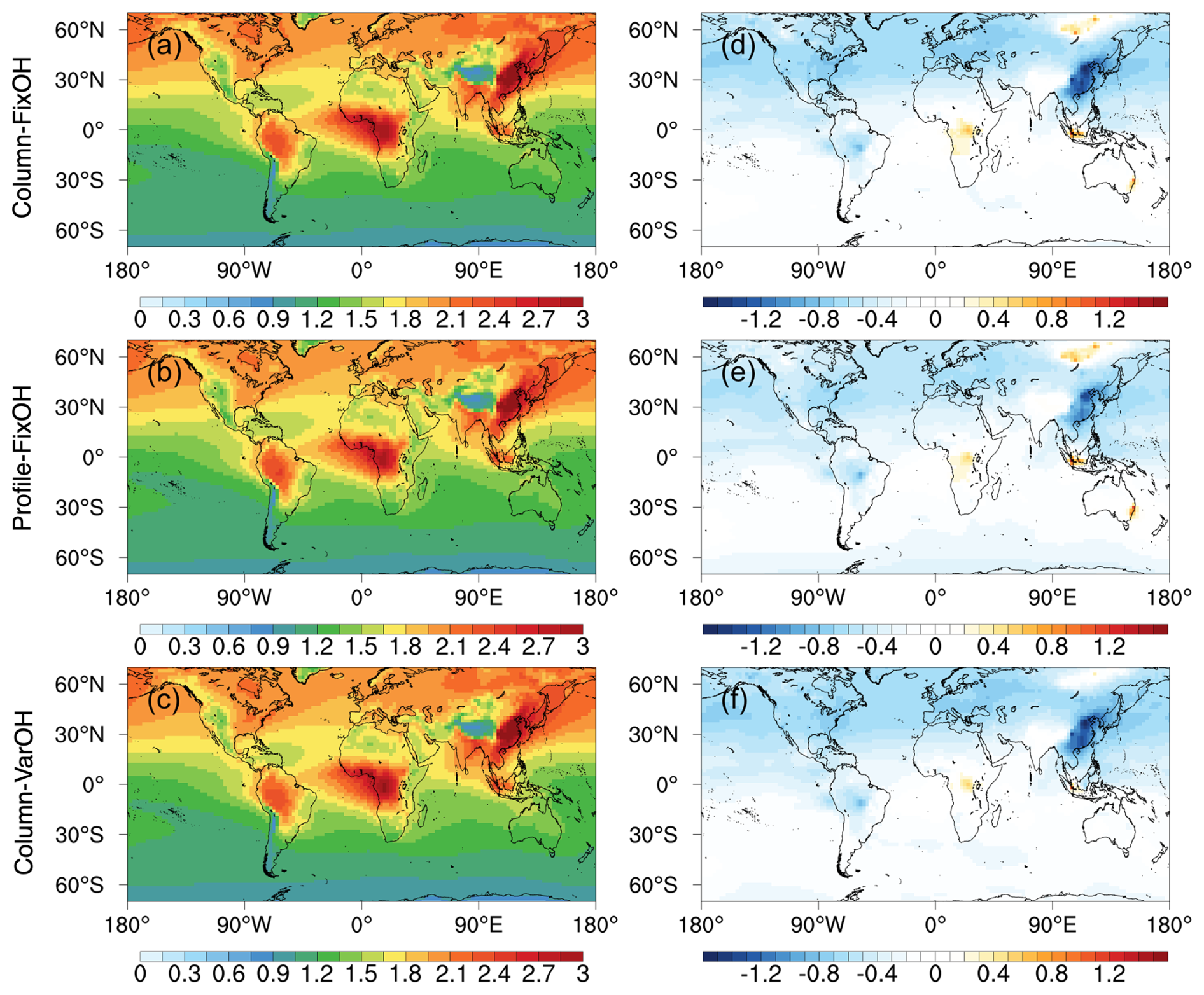
Figure 9 Modeled column CO concentrations (10¹⁸ $\mathrm{molec}.{\mathrm{cm}}^{-\mathrm{2}}$) and their trends (% yr⁻¹) from 2003 to 2022. (a–c) Spatial distribution of the 20 year mean. (d–f) Spatial pattern of the long-term trend.

To quantitatively attribute the concentration trends to specific drivers, we conducted a series of sensitivity experiments. The experimental design isolates the influence of individual emission sectors by building a baseline scenario in which all emissions are fixed at 2003 levels to reflect the impact of meteorological condition changes in 2003–2022. Three more sensitivity experiments were then conducted in 2003–2022 in which only one emission category, i.e., anthropogenic, biomass burning, or biogenic VOC sources, was allowed to vary over time, respectively. The time-varying sources in these sensitivity experiments were prescribed from the Column-FixOH a posteriori inversion.

The results indicate that meteorological influences induced positive trends in surface CO concentrations in regions such as central Africa, Southeast Asia, and the Tibetan Plateau (0.6 %–1.8 % yr⁻¹), along with slight negative trends in areas such as South America (Fig. 10a). The meteorological impact on CO column concentrations was comparatively weaker (Fig. 10b), showing positive trends of 0.45 % yr⁻¹ over central Africa and the Tibetan Plateau. This vertical differentiation implies that meteorological influences may primarily alter the vertical distribution of CO through changes in convective transport, with a more limited effect on larger horizontal scales. The derived meteorological impact is noticeably weaker than that reported by Jiang et al. (2017), a discrepancy likely attributable to our use of consistent MERRA-2 meteorological fields, which enhances the reliability of the long-term trend analysis. Similarly, the impact of biogenic VOC changes on CO concentrations (Fig. 10g and h) was markedly weaker than in Jiang et al. (2017).

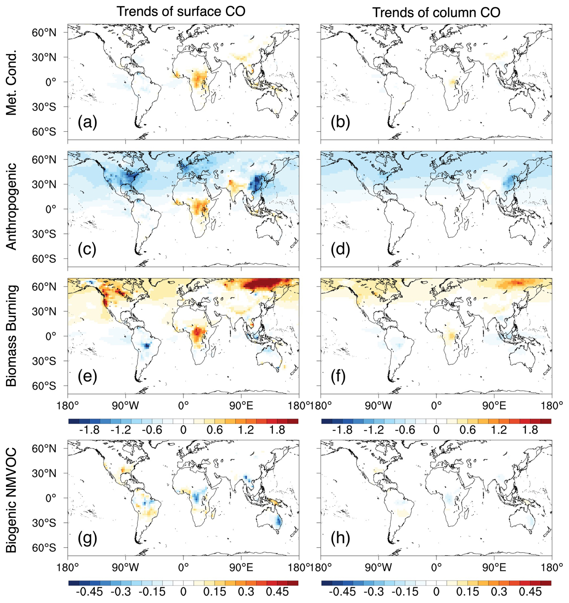
Figure 10 Attribution of trends (% yr⁻¹) in surface and column CO concentrations to individual drivers, derived from sensitivity simulations based on Column-FixOH inversion (2003–2022). Trends are shown for scenarios with: (a, b) all sources fixed at 2003 levels; (c, d) only anthropogenic emissions varying over time; (e, f) only biomass burning emissions varying; (g, h) only biogenic VOC sources varying.

Table 4 Attribution of trends in column CO concentrations (% yr⁻¹) from 2003 to 2022 to changes in anthropogenic and biomass burning emissions, based on sensitivity simulations using the Column-FixOH inversion results.

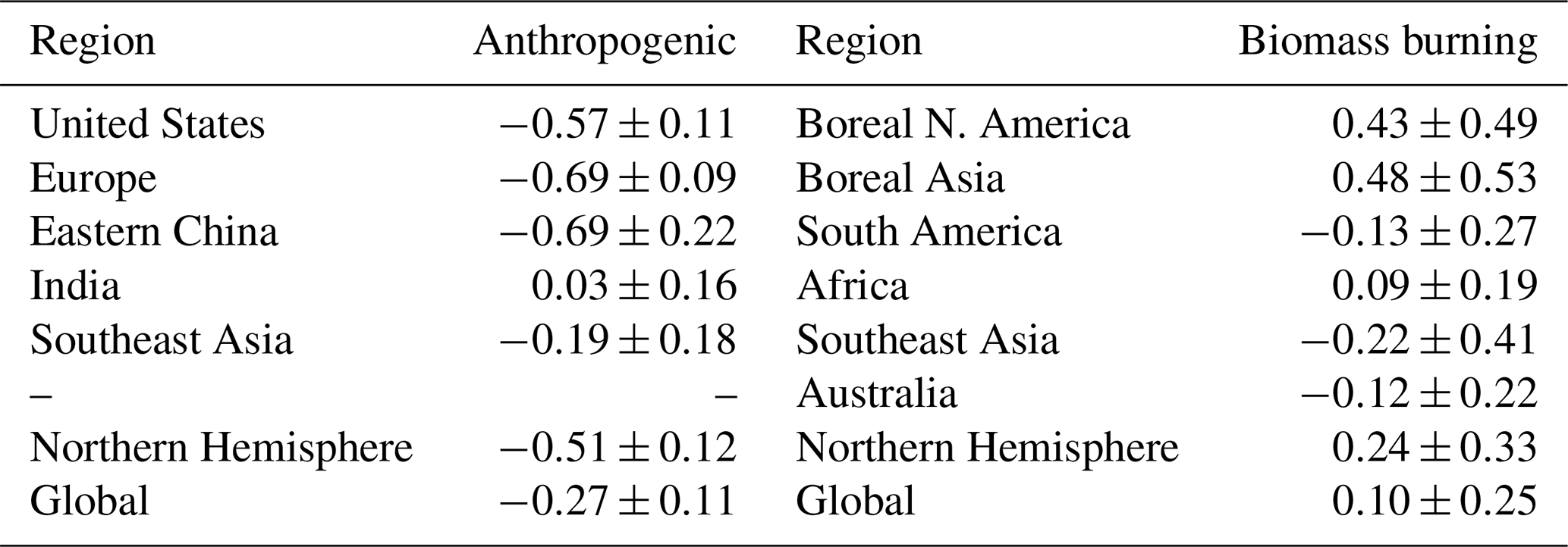
Anthropogenic emission changes were identified as the principal driver behind declining CO levels, inducing strong negative trends in industrial regions of the Northern Hemisphere, such as eastern North America, Europe, and eastern China. This signal is consistent across both surface and column concentrations (Fig. 10c and d). Globally, anthropogenic emission changes led to an average annual decrease of 0.27 % yr⁻¹ in CO column concentrations, with a more pronounced decline rate of 0.51 % yr⁻¹ in the Northern Hemisphere (Table 4). Regionally, the US, Europe, and eastern China exhibited the most substantial decreases, at −0.57 % yr⁻¹, −0.69 % yr⁻¹ and −0.69 % yr⁻¹, respectively. In contrast, India experienced a slight concentration increase (0.03 % yr⁻¹) due to rising emissions, while Southeast Asia showed a more moderate decline (−0.19 % yr⁻¹) compared to other major industrial regions.

Conversely, changes in biomass burning emissions generally contributed to positive trends in CO, particularly at high latitudes (Fig. 10e and f). At global and Northern Hemispheric scales, this positive trend was largely attributable to extreme wildfire activity in 2021. When 2021 is excluded, the long-term trend in CO columns due to biomass burning becomes statistically insignificant at these broad scales (Fig. 7g and h), with only regionally and seasonally confined increases remaining apparent, notably over Boreal Asia (July–August, Fig. 7b) and Africa (January–April, Fig. 7d). In the full record (including 2021), biomass burning emissions led to an average annual increase of 0.10 % yr⁻¹ in global CO columns, and 0.24 % yr⁻¹ in the Northern Hemisphere (Table 4). It is noteworthy that the CO concentration response lagged behind emission pulses by about one month and persisted longer. In the Northern Hemisphere, for instance, enhanced emissions occurred mainly from July to September, whereas the significant concentration response extended from August to December (Fig. 7g). This lag and prolonged influence were primarily attributable to the delayed response over Boreal North America (Fig. 7a). At the regional scale, increases occurred in Boreal North America (0.43 % yr⁻¹) and Boreal Asia (0.48 % yr⁻¹). In contrast, South America, Australia, and Southeast Asia experienced declining trends ranging from −0.13 % yr⁻¹ to −0.22 % yr⁻¹, while Africa showed a slight increase of 0.09 % yr⁻¹.

This attribution analysis highlights the substantial impact of extreme wildfire years on the CO budget. Although anthropogenic emission reductions lowered Northern Hemisphere CO columns by approximately 0.51 % yr⁻¹, the intense biomass burning emissions in 2021 introduced a positive perturbation of about 0.24 % yr⁻¹ in the full-record trend, thereby offsetting a considerable fraction of the anthropogenic-driven decline. As a result, the net concentration decline was reduced to approximately 0.27 % yr⁻¹ in the analysis including 2021. This implies that nearly half (47 %) of the potential air quality improvement from anthropogenic emission controls can be offset by wildfire emissions. This finding provides a clear mechanistic explanation for the decline in atmospheric CO concentrations in recent years, and underscores the growing role of extreme wildfire events in modulating regional to hemispheric air composition.

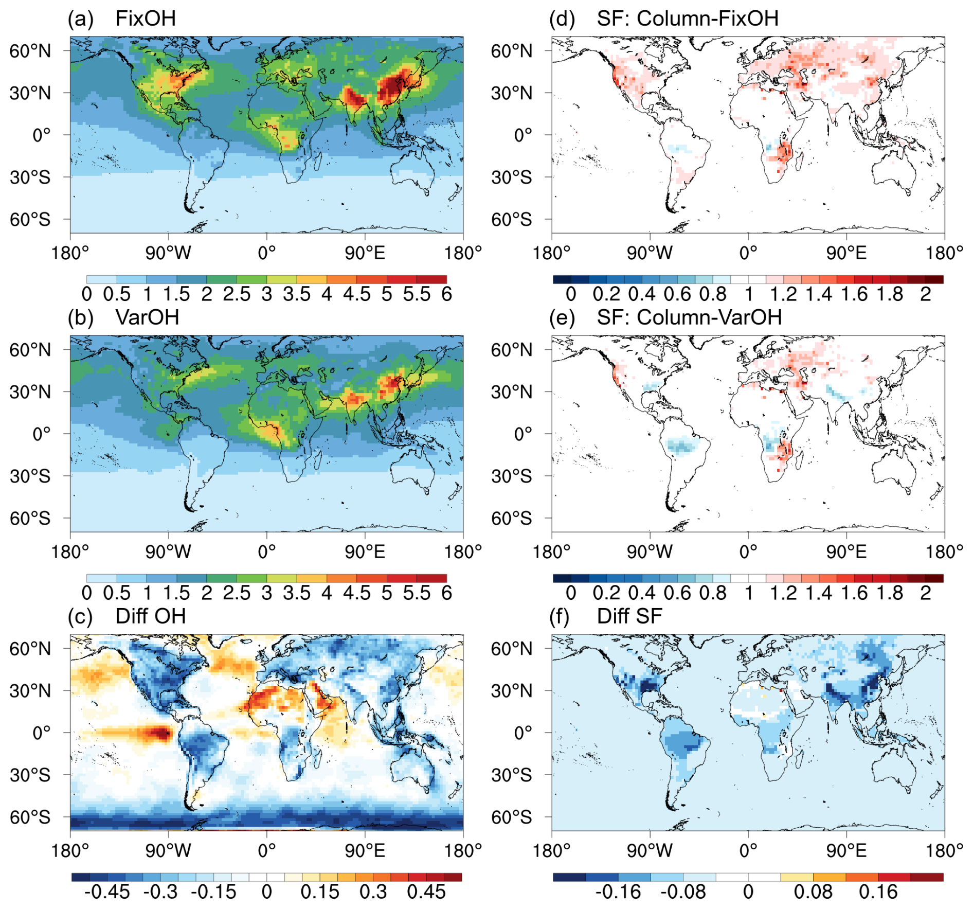
Figure 11 Sensitivity of inverted CO emissions to OH fields. (a–c) Tropospheric OH columns (10¹² $\mathrm{molec}.{\mathrm{cm}}^{-\mathrm{2}}$) from fixed and variable (TCR-2) fields and their difference. (d–f) Corresponding scaling factors from the Column-FixOH and Column-VarOH inversions and their difference. Please note that due to the use of land boundary conditions, differences in OH concentrations over the ocean in the left column figures have a negligible effect on the differences in scaling factors shown in the right column figures.

3.4 Impacts of systematic errors on inferred CO emissions

The MOPITT instrument provides retrievals for both CO total column and vertical profile. The degrees of freedom for signal (DFS) for MOPITT multi-spectral profile retrievals (TIR + NIR) is approximately 1.5–2.0 over land, reducing to about 1.0 when converted to a total column (Worden et al., 2010). The discrepancy between a posteriori emission estimates constrained by CO column (Column-FixOH) and profile (Profile-FixOH) data helps evaluate the influence of systematic errors associated with the vertical sensitivity of the satellite retrievals (Tang et al., 2024). Globally, a posteriori anthropogenic and biomass burning CO emissions from Profile-FixOH were both slightly lower than those from Column-FixOH, with average differences of −6.6 % and −5.5 %, respectively, over the period 2003–2022 (Table 2). The two configurations also showed broadly consistent long-term trends in inferred anthropogenic emissions, both indicating a global decline of approximately −0.9 % yr⁻¹. Larger regional discrepancies were observed over eastern China (−2.1 % yr⁻¹ for Profile-FixOH vs. −1.6 % yr⁻¹ for Column-FixOH) and India (1.1 % yr⁻¹ vs. 0.7 % yr⁻¹). Similarly, the trends in global biomass burning CO emissions were consistent (0.3 % yr⁻¹ for Column-FixOH and 0.5 % yr⁻¹ for Profile-FixOH), though regional differences were more pronounced for boreal North America (3.1 % yr⁻¹ vs. 4.9 % yr⁻¹) and Australia (−1.5 % yr⁻¹ vs. −0.7 % yr⁻¹). The limited differences in inferred emissions between the two configurations resulted in a consistent declining trend in simulated CO columns (−0.5 % yr⁻¹ for both).

OH concentrations in model simulations significantly influence the inverse analysis of CO emissions (Jiang et al., 2011; Müller et al., 2018). By assimilating MOPITT CO column data, we compared the inverted CO emission estimates driven by fixed (Column-FixOH) and variable (Column-VarOH) OH fields to investigate the potential influence. As shown in Fig. 11c, OH concentrations from the TCR-2 reanalysis are broadly 10 %–40 % lower than the fixed climatological OH concentrations over land (differences over the ocean are not considered here due to the use of CO land boundary conditions in the 4D-Var assimilation). Lower OH concentrations over land lead to reduced chemical loss, which is compensated by lower global anthropogenic CO emissions in Column-VarOH inversion (590.1 Tg yr⁻¹) in 2003–2022, approximately 3.7 % lower than in Column-FixOH (612.8 Tg yr⁻¹).

Variations in OH concentrations influence the oxidation of biogenic VOCs to CO and their subsequent chemical loss. These two counteracting processes establish a complex balance, ultimately reflected in the inverted estimates of biogenic CO sources. Specifically, the Column-VarOH inversion yields an average global biogenic CO sources of 391.4 Tg yr⁻¹ in 2003–2022, approximately 3.9 % lower than the 407.6 Tg yr⁻¹ in Column-FixOH inversion. The sensitivity experiments described above address the third objective of this study, which is to evaluate the robustness of our central findings against potential systematic errors associated with satellite retrieval vertical sensitivity and OH concentrations. This robustness can be attributed, in part, to our two-step inversion framework, which mitigates systematic biases through optimized initial and boundary CO conditions.

4 Conclusions

This study provides a comprehensive, quantitative analysis of global CO emissions and drivers governing atmospheric CO trends over the past two decades (2003–2022). By employing a 4D-Var assimilation framework within GEOS-Chem adjoint model, constrained by long-term MOPITT satellite measurements, we have generated an observationally constrained CO emission inventory. A central methodological strength lies in the use of continuous MERRA-2 meteorological fields and modern a priori emission inventories, which significantly enhanced the long-term consistency and reliability of our trend analysis. The implementation of a two-step bias mitigation strategy, optimizing both initial conditions and land boundary conditions for CO, effectively reduced the accumulated impacts of transport and chemistry uncertainties. The optimized emissions yield simulated CO concentrations that show good agreement with independent surface measurements from the WDCGG network and aircraft-based profiles from the HIPPO and ATom campaigns. The mean bias in simulated CO concentrations (model minus observation) was reduced from −3.8 ppb in a priori simulation to between −2.5 and −2.1 ppb in a posteriori simulation for HIPPO, and from −3.4 ppb in a priori simulation to between −2.9 and −1.6 ppb in a posteriori simulation for ATOM.

Our results demonstrate a significant 14 %–17 % decline (approximately 85–110 Tg yr⁻¹) in global anthropogenic CO emissions over the 20 year period. This reduction was predominantly driven by pollution control policies in major industrialized regions, with cumulative reductions of 46 %–49 % in the US, 32 %–34 % in Europe, and 23 %–32 % in eastern China. The decline in anthropogenic CO emissions is consistent with the trends reported in the CEDS-CMIP7 inventory and the inversion results of Zheng et al. (2019), and is identified as the dominant and statistically significant driver behind the observed decrease in atmospheric CO concentrations. For biomass burning, our emission estimates suggested the historical peak of approximately 500 Tg yr⁻¹ in 2021, while the overall CO emissions in GFED5 inventory are higher than our estimates in 2003–2022. Biomass burning emissions exhibited strong interannual variability without a statistically significant long-term trend at the global and Northern Hemispheric scales, although regionally and seasonally trends, such as in the boreal Northern Hemisphere during summer, were evident in certain periods.

A central finding of this work is the substantial impact of extreme wildfire events, particularly the record-breaking 2021 burning season in Northern Hemisphere high latitudes. Our attribution analysis reveals that these wildfires introduced a strong positive perturbation to atmospheric CO, offsetting nearly half (47 %) of the concentration decline driven by anthropogenic reductions in the Northern Hemisphere over our study period (2003–2022). This finding highlights that while not a persistent trend, extreme wildfire events can counteract a large fraction of the gains achieved from decades of emission control efforts. Our analysis thus clarifies the past evolution of global CO emissions and concentrations, highlighting an increasingly critical challenge: climate change is amplifying the intensity and impact of extreme wildfire events, which can periodically undermine emission control efforts. This underscores the need for integrated policies that address both anthropogenic sources and the climate-driven amplification of natural emissions.