2019–2024 trends in African livestock and wetland emissions as contributors to the global methane rise

The African continent has been recognized as a major driver of the recent rise in atmospheric methane, but the causes are not well understood. Here we use blended TROPOMI+GOSAT satellite observations of methane to quantify and attribute African emission trends over August 2018–December 2024. We do this with monthly analytical inversions, optimizing surface fluxes at 50 km resolution on the continental scale and using two alternative bottom-up wetland emission models (WetCHARTs-CYGNSS and LPJ-EOSIM-MERRA2) as prior estimates. Our best estimate of total surface fluxes from Africa over the 2019–2024 period is 71–72 Tg a⁻¹ depending on the choice of prior wetland emission estimate, including 28–32 Tg a⁻¹ from wetlands and 23–25 Tg a⁻¹ from livestock. We find that the bottom-up models greatly underestimate wetland emissions in South Sudan and Lake Chad and greatly overestimate emissions in the Congo Basin. Annual methane surface fluxes from Africa increased by 19–21 Tg a⁻¹ over 2019–2024, contributing 27 % of the global emission increase in 2019–2021 and continuing to increase after 2021 even as global emissions decreased. The 2019–2024 increase in African emissions included 11 Tg a⁻¹ from livestock, 4.3–5.7 Tg a⁻¹ from wetlands, and 2.5–2.8 Tg a⁻¹ from waste. The increase in livestock emissions was steady while wetland emissions surged in 2020 and 2024. Previous studies attributed uncertainties in bottom-up wetland data to poor information on inundation extent, but we find that the CYGNSS satellite inundation data match the spatial, seasonal, and interannual patterns of our optimized wetland emissions.

1 Introduction

Rising atmospheric methane concentrations have contributed 30 % of observed warming since pre-industrial times (Szopa et al., 2021). Isotopic data indicate that the methane rise over the past two decades has been driven by microbial sources in the tropics that could include wetlands, livestock, and waste (Nisbet et al., 2023; Drinkwater et al., 2023). The rise has accelerated over the past decade to a record rate of 15 ppb a⁻¹ in 2020–2022 with a correspondingly large isotopic shift (Michel et al., 2024) before slowing down to 8 ppb a⁻¹ in 2023–2024. Global satellite observations of total column methane from GOSAT (2009–present) and TROPOMI (2018–present) are a unique resource for monitoring and attributing methane emissions worldwide (Jacob et al., 2022). Inverse analyses combining the satellite data with an atmospheric transport model can provide optimized estimates of emissions and their trends (Jacob et al., 2016). Bottom-up estimates derived from activity data and emission factors regularize these inversions and provide a transparent link to the underlying processes. Inverse analyses of satellite data have identified Africa as a large and increasing source of methane, and the largest driver in the recent acceleration of the methane rise (Feng et al., 2023; He et al., 2025). Air pollution-modulated changes in hydroxyl radical concentrations also impact the methane growth rate (Laughner et al., 2021; Stevenson et al., 2022; Peng et al., 2022; Zhao et al., 2025; Yoon et al., 2025, Ciais et al., 2026).

The increase in African methane emissions has been attributed to precipitation-driven expansion of wetlands in East Africa (Qu et al., 2022; Feng et al., 2022), with evidence from the GRACE-FO satellite instrument of increases in total water storage (Lunt et al., 2021; Feng et al., 2023; Qu et al., 2024; Lin et al., 2024; Pendergrass et al., 2025). However, there are problems with this attribution. The locations of increasing emissions identified by satellite coincide more with livestock than wetlands (Pendergrass et al., 2025). Bottom-up wetland models do not show increasing emissions in Africa in recent years (Lin et al., 2024). Surface inundation data from the CYGNSS satellite constellation also do not show an increase (Xiong et al., 2025), in contrast to GRACE-FO observations. GRACE-FO total water storage includes both surface and ground water (Boergens et al., 2024), complicating its interpretation as a wetland inundation metric. Livestock populations in Africa are growing rapidly (Zhang et al., 2021; Tang et al., 2025), which could be an alternative explanation for the rise in African methane emissions.

Besides wetlands and livestock, other sectors contributing to methane surface fluxes in Africa include waste, soil uptake, oil and gas, termites, fires, and rice (Saunois et al., 2025). Uptake of methane by soil methanotrophs is disperse but significant, with large uncertainties over tropical forests (Murguia-Flores et al., 2018; Jiang et al., 2025). Oil and gas emissions are predominantly from Nigeria, Algeria, and Angola (Scarpelli et al., 2025; Chen et al., 2023; Western et al., 2021; Fiehn et al., 2025; Naus et al., 2023; Schuit et al., 2023). Rice cultivation has been increasing in Africa (Chen et al., 2024).

Here, we quantify and attribute the rise in African methane emissions from August 2018 to December 2024 by combining TROPOMI satellite observations with bottom-up surface flux estimates in monthly analytical inversions using detailed prior error covariances. We use two different bottom-up wetland models, WetCHARTs-CYGNSS and LPJ-EOSIM-MERRA2, as alternative estimates for the wetland portion of our prior estimate. We optimize methane surface fluxes at 50 km and monthly resolution, allowing better separation of emissions from different sectors than previous coarser-resolution inversions, and avoiding errors from incorrect seasonality in the prior estimates. As we will see, the multi-year TROPOMI record enables us to quantify African emissions with little dependence on the prior estimates and thus enables us to use the inversion results not only to explain emission trends but also to provide guidance for improving wetland models.

2 Data and methods

We use Bayesian optimal estimation to retrieve monthly mean methane surface fluxes (net sum of emission and uptake) at 0.5° × 0.625° (≈ 50×50 km²) resolution over the African continent (19.375° W–53.125° E, 37.0° S–40.5° N, domain shown in Fig. 1) using TROPOMI methane concentrations and the nested GEOS-Chem atmospheric transport model to relate surface fluxes to concentrations. We minimize the Bayesian cost function

$$\begin{array}{}\text{(1)}& \begin{array}{rl}J\left(\mathit{x}\right)& ={\left(\mathit{x}-{\mathit{x}}_{\mathrm{a}}\right)}^{\top }{\mathbf{S}}_{\mathrm{a}}^{-\mathrm{1}}\left(\mathit{x}-{\mathit{x}}_{\mathrm{a}}\right)\\ & +{\left(\mathit{y}-F\left(\mathit{x}\right)\right)}^{\top }{\mathbf{S}}_{\mathrm{o}}^{-\mathrm{1}}\left(\mathit{y}-F\left(\mathit{x}\right)\right)\end{array}\end{array}$$

to optimize a state vector x of monthly mean surface fluxes (µg m⁻² s⁻¹) from 10 768 land and offshore grid cells and 6 boundary conditions (ppb) including for the northern and southern boundaries, and for the western and eastern boundaries separately north and south of the Equator. J(x) balances deviations of the solution x from the prior estimate x_a and from TROPOMI observations y as simulated by GEOS-Chem (F(x)), with weighting by the prior and observing system error covariance matrices S_a and S_o and assuming normal error probability density functions. Our GEOS-Chem simulation responds linearly to perturbations in x and thus can be represented by the Jacobian matrix $\mathbf{K}=\partial \mathit{y}/\partial \mathit{x}$. This permits an analytical solution for the optimal estimate $\widehat{\mathit{x}}$ (Rodgers, 2000).

$$\begin{array}{}\text{(2)}& \widehat{\mathit{x}}={\mathit{x}}_{\mathrm{a}}+{\left({\mathbf{K}}^{\top }{\mathbf{S}}_{\mathrm{o}}^{-\mathrm{1}}\mathbf{K}+{\mathbf{S}}_{\mathrm{a}}^{-\mathrm{1}}\right)}^{-\mathrm{1}}{\mathbf{K}}^{\top }{\mathbf{S}}_{\mathrm{o}}^{-\mathrm{1}}\left(\mathit{y}-F\left({\mathit{x}}_{\mathrm{a}}\right)\right)\end{array}$$

We run 77 months of sequential monthly analytical inversions (August 2018–December 2024). Unlike annual inversions, this approach avoids imposing seasonality from the bottom-up estimates. The prior estimate for each month is informed by both the bottom-up surface flux estimates for that month and the optimal surface fluxes from the previous month in a framework similar to Varon et al. (2023).

$$\begin{array}{}\text{(3)}& {\mathit{x}}_{\mathrm{a}}=\mathit{\lambda }\left({\mathit{x}}_{\mathrm{b},t}+{\widehat{\mathit{x}}}_{t-\mathrm{1}}^{\ast }\right)\end{array}$$

Here, x_a is the prior state estimate for month t, x_b,t is the bottom-up surface flux estimate for month t, and ${\widehat{\mathit{x}}}_{t-\mathrm{1}}^{\ast }$ is a modified form of the optimal state from month t−1 that (1) replaces flux values below −0.025 µg m⁻² s⁻¹ with that limit to avoid surface flux dipoles symptomatic of overfit, and (2) resets boundary condition corrections to 0 ppb. The factor λ sets the domain-wide flux for x_a to that of ${\widehat{\mathit{x}}}_{t-\mathrm{1}}$, the unmodified optimal state from month t−1. For the first month of August 2018, x_b,t is used for x_a. We run two independent sets of monthly inversions, varying the bottom-up representation of wetlands, using either observed inundation (WetCHARTs-CYGNSS) or a reanalysis-informed model (LPJ-EOSIM-MERRA2), described below. Though our state vector includes part of the Middle East and southern Europe, we restrict our analysis to Africa.

2.1 TROPOMI satellite observations and the GEOS-Chem model

Our observing system consists of the TROPOMI satellite observations and the GEOS-Chem atmospheric transport model. The TROPOMI satellite instrument retrieves column-average dry-air methane mixing ratios (XCH₄) at a 5.5 × 7 km² nadir spatial resolution (7 × 7 km² before August 2019) from solar backscatter radiance measurements in the 2.3 µm methane absorption band (Hu et al., 2018). These observations cover the globe each day with a 3 % global retrieval success rate limited by clouds, dark or heterogeneous surfaces, and topography.

We use the blended TROPOMI+GOSAT XCH₄ product (Balasus et al., 2023), accessed from https://registry.opendata.aws/blended-tropomi-gosat-methane/ (last access: 22 October 2025) and refer to it as TROPOMI for brevity. This product starts with the operational TROPOMI product from the Space Research Organisation Netherlands (Lorente et al., 2023) and corrects it using machine learning with co-located retrievals from GOSAT. The GOSAT observations are less subject to biases than TROPOMI owing to higher spectral resolution and use of a CO₂ proxy retrieval method (Parker et al., 2020), but they are also much sparser. We use only land observations and filter out coastal scenes with poor spectral fits (Balasus et al., 2023). We average together individual observations taken on the same orbit within the same 0.5° × 0.625° grid cell to make super-observations (Eskes et al., 2003; Chen et al., 2023) which populate our observation vector y.

Figure 1 shows TROPOMI super-observations of XCH₄ averaged across August 2018–December 2024, containing 269 million individual TROPOMI observations. The north-south XCH₄ gradient is driven by the global background. Concentrations are highest over the Sudd wetlands of South Sudan, the Niger Delta with its combination of wetlands and oil and gas production, and an equatorial band though with few observations due to clouds and optically dark tropical forests.

We use version 14.5.0 of the GEOS-Chem chemical transport model (Maasakkers et al., 2019) with the TROPOMI operator (Varon et al., 2022) to relate surface fluxes to the TROPOMI observations. The model is driven by assimilated meteorological data from the MERRA-2 reanalysis and has a spatial resolution of 0.5° × 0.625°, the same as our state vector, with 72 vertical layers. The model includes chemical loss of methane using archived oxidant fields (Wecht et al., 2014). We use the nested version of GEOS-Chem over Africa with dynamic boundary conditions updated every 3 h. The boundary conditions are imposed by smoothed TROPOMI concentration fields so as to be unbiased relative to the observations (Estrada et al., 2025). They are constructed by (1) conducting a global GEOS-Chem simulation at 2.0° × 2.5° resolution using MERRA-2 meteorology, (2) smoothing the 2.0° × 2.5° average daily differences between GEOS-Chem and TROPOMI column concentrations spatially within 10° × 12.5° domains and temporally across ±15 d, filling gaps over oceans with latitudinal averages, and (3) scaling the original GEOS-Chem vertical profiles to remove the smoothed bias relative to TROPOMI column concentrations. The boundary condition elements of our state vector are an additive correction to these boundary conditions.

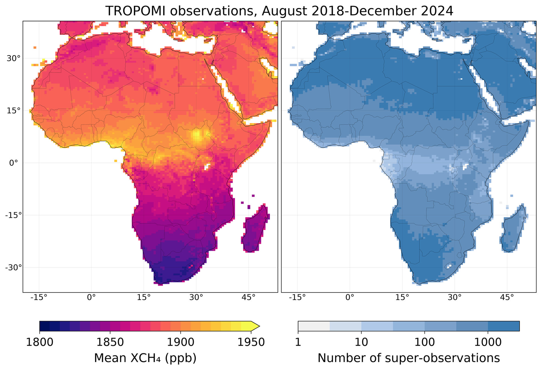
Figure 1 TROPOMI satellite observations of methane over Africa for August 2018–December 2024. Super-observations are shown, defined by averaging together observations taken on the same orbit within the same 0.5°×0.625° grid cell. The left panel shows the mean column-average dry-air methane mixing ratios (XCH₄) from the Balasus et al. (2023) blended product. The right panel shows the number of super-observations per grid cell on a log scale. Areas in white have no observations.

We take the observing system covariance matrix S_o to be diagonal with GEOS-Chem transport error variance and TROPOMI super-observation error variance added in quadrature. The transport error standard deviation is taken to be 4 ppb as inferred by Hancock et al. (2025) from the residual error method in the asymptote of high observation density (Chen et al., 2023). The uncertainties reported in the operational TROPOMI product for individual observations, propagated from noise in the spectral measurements, do not reflect the total observation error because they do not account for retrieval error (Sicisk-Paré et al., 2025). Following Schneising (2025), we incorporate retrieval error by using ground-based XCH₄ observations from TCCON stations worldwide (Wunch et al., 2011). Using August 2018–December 2024 TROPOMI XCH₄ for 26 GGG2020 TCCON stations (https://tccondata.org, last access: 21 July 2025) as in Balasus et al. (2023), we derive the TROPOMI precision at each of the 26 TCCON stations and then regress these station precisions against the average operationally-reported uncertainty for TROPOMI at each station (slope = 1.8, intercept = 8.0 ppb, Pearson's r=0.7) as shown in Fig. 2. We use this fit to translate from the operationally-reported uncertainty to individual observation error standard deviations σ_i for each TROPOMI observation i. The error variance for a super-observation ${\mathit{\sigma }}_{\mathrm{super}}^{\mathrm{2}}$ is a function of the individual error standard deviations σ_i of the N observations averaged together to make the super-observation and a representative uniform correlation coefficient c as in Eq. (4) following Rijsdijk et al. (2025).

$$\begin{array}{}\text{(4)}& {\mathit{\sigma }}_{\mathrm{super}}^{\mathrm{2}}={\displaystyle \frac{\mathrm{1}}{N^{\mathrm{2}}}}\left[\left(\mathrm{1}-c\right)\sum _{i=\mathrm{1}}^N{\mathit{\sigma }}_i^{\mathrm{2}}+c{\left(\sum _{i=\mathrm{1}}^N{\mathit{\sigma }}_i\right)}^{\mathrm{2}}\right]\end{array}$$

Using data from all TCCON stations, we find that the variance of TROPOMI super-observation residuals (TROPOMI-TCCON-mean station bias) best fit Eq. (4) using a correlation coefficient c=0.3 (also shown in Fig. 2).

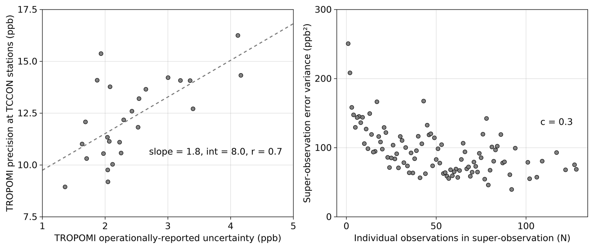
Figure 2 Determination of TROPOMI super-observation error variances using TCCON ground-based column data. The left panel shows a linear regression of the TROPOMI precision (error standard deviation) at 26 TCCON stations against the average operationally-reported TROPOMI uncertainty at each of those stations (slope, intercept, and Pearson's r inset). The right panel shows the super-observation error variance at TCCON sites versus the number of individual observations contributing to the super-observation, featuring an asymptote that corresponds to a correlation coefficient of 0.3 in Eq. (4). The analysis uses TROPOMI data coincident with TCCON data, defined as being within 100 km from the TCCON site (except for 50 km for the Edwards site), no more than 250 m in elevation difference, and within 1 h of the TCCON observation (Balasus et al., 2023).

2.2 Prior surface flux estimates

Table 1 lists continental totals for the gridded bottom-up methane surface fluxes used as our prior estimates. These are resolved by sector and include both natural (wetlands, soil uptake, termites, fires, geological seeps) and anthropogenic (livestock, waste, oil, gas, rice, coal) categories. Wetlands and livestock dominate.

Table 1 Bottom-up methane surface fluxes from Africa (Tg a⁻¹)^*.

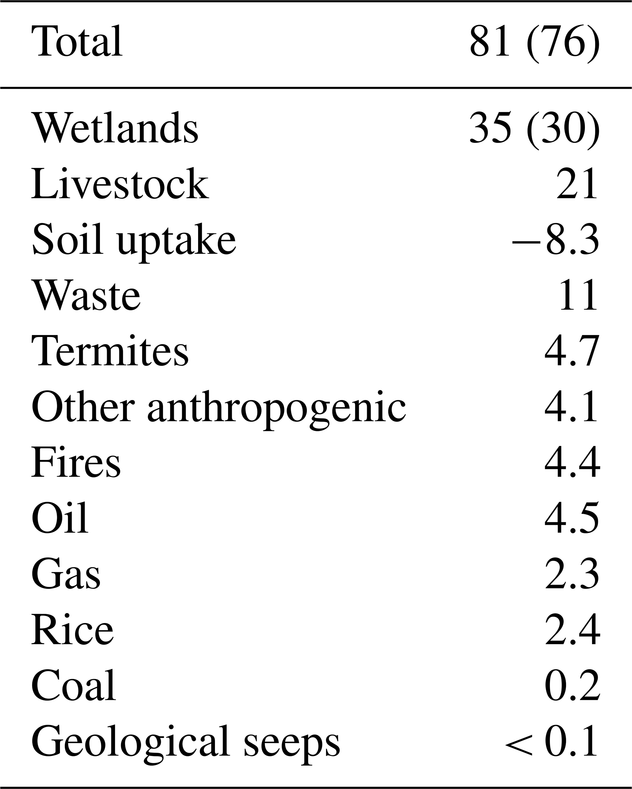
^* Continental 2019–2024 averages for the gridded bottom-up fluxes used as prior estimates in the inversion. Wetlands are from WetCHARTs-CYGNSS as described in the text (LPJ-EOSIM-MERRA2 in parentheses). Livestock (enteric fermentation and manure management), waste (landfills and wastewater treatment), and other anthropogenic sources (residential energy, transportation, and industry) are from the Emissions Database for Global Atmospheric Research (EDGARv8, Crippa et al., 2024). Soil uptake is from MeMo v1.0 (Murguia-Flores et al., 2018). Termite emissions are from Ito (2023). Open fire emissions are from the Global Fire Emissions Database (GFEDv4.1s, van der Werf et al., 2017). Oil, gas, and coal emissions are from the Global Fuel Exploitation Inventory (GFEIv3, Scarpelli et al., 2025). Rice emissions are from the Global Rice Paddy Inventory (GRPI, Chen et al., 2025). Seep emissions are based on the global annual total of Hmiel et al. (2020) distributed spatially following Etiope et al. (2019) and are negligible in Africa.

We use two alternative bottom-up wetland representations for the inversion, WetCHARTs-CYGNSS and LPJ-EOSIM-MERRA2 (Zhang et al., 2023; Colligan et al., 2024; Quinn et al., 2025), to test the sensitivity of inversion results to the specification of the prior estimate. We build WetCHARTs-CYGNSS here, following Gerlein-Safdi et al. (2021), Li et al. (2024), and Xiong et al. (2025). WetCHARTs is an empirical framework for estimating methane emissions based on wetland extent, heterotrophic respiration, and temperature (Bloom et al., 2017). Default wetland extent in the WetCHARTs extended ensemble is based on static wetland charts scaled monthly based on precipitation. Instead, we use observed inundation from CYGNSS, a constellation of satellites that can use GPS signals to map inland water extent, seeing through vegetation and clouds. We use the monthly CYGNSS Berkeley-RWAWC product (Pu et al., 2024) for inundation at 0.01° × 0.01° resolution. Pairing this with a scale factor setting global wetland methane emissions to 207.5 Tg in 2019, a 2001–2021 climatology of CARDAMOM respiration, and no temperature dependence for the methane $/$ CO₂ respiration ratio (WetCHARTs ensemble member 3914 that East et al. (2024) identified as best-performing), we produce WetCHARTs-CYGNSS at 0.5° × 0.5° for each month from August 2018 to December 2024. All high-performing WetCHARTs ensemble members use CARDAMOM respiration (Ma et al., 2021). LPJ-EOSIM-MERRA2 is a land surface model that uses reanalysis meteorological data to quantify wetland emissions. We choose this model as an alternative to WetCHARTs-CYGNSS in our sensitivity inversion because it provides a good match to the observed seasonality in background methane concentrations (East et al., 2024).

Figure 3 shows total bottom-up methane surface fluxes as 2019–2024 averages, differing only in their wetland component. Wetlands and livestock are shown individually in Fig. 4. WetCHARTs-CYGNSS has more expansive wetlands with lower magnitude emissions than LPJ-EOSIM-MERRA2, especially in the Congo Basin. The lower magnitude emissions from the Congo Basin in WetCHARTs-CYGNSS, which come about from lower inundation than other inventories (Zhu et al., 2025), are supported by GOSAT observations (Lunt et al., 2019; Maasakkers et al., 2019). Livestock emissions are almost entirely from enteric fermentation and are concentrated in Ethiopia, Kenya, and the Sahel. Localized livestock emission hotspots in Morocco, South Africa, and Somalia stem from an EDGARv8 spatialization method that uses satellite-observed ammonia hotspots (Crippa et al., 2024). Soil uptake is diffuse throughout the continent except in the central Sahara. Waste emissions are in and around urban areas. Oil and gas emissions are mainly from Nigeria, Angola, and Algeria.

We construct the prior error covariance matrix S_a by assuming 50 % relative error standard deviations on the flux elements of x_a. Then, S_a is constructed element-by-element for $j\in \mathit{\{}\mathrm{1},\mathrm{2},\mathrm{\dots },\mathrm{10}\mathrm{768}\mathit{\}}$ and $k\in \mathit{\{}\mathrm{1},\mathrm{2},\mathrm{\dots },\mathrm{10}\mathrm{768}\mathit{\}}$ as

$$\begin{array}{}\text{(5)}& {\mathbf{S}}_{\mathrm{a}}\left[j,k\right]=\exp \left(-d/l\right)\times s\times {\mathit{\sigma }}_j\times {\mathit{\sigma }}_k\end{array}$$

where σ_j is the error standard deviation for grid cell j, d is the distance between the grid cells in km, l is an error correlation length scale of 200 km (Yu et al., 2021), and s is the cosine similarity between vectors of the bottom-up sectoral composition for the grid cells, following on work from Turner et al. (2020). The scheme yields large error correlations between grid cells that are physically close and have similar sectoral attributions. Boundary condition corrections are given an error variance of 100 ppb² with no error correlations. We construct S_a in this manner for each month based on x_a from Eq. (3).

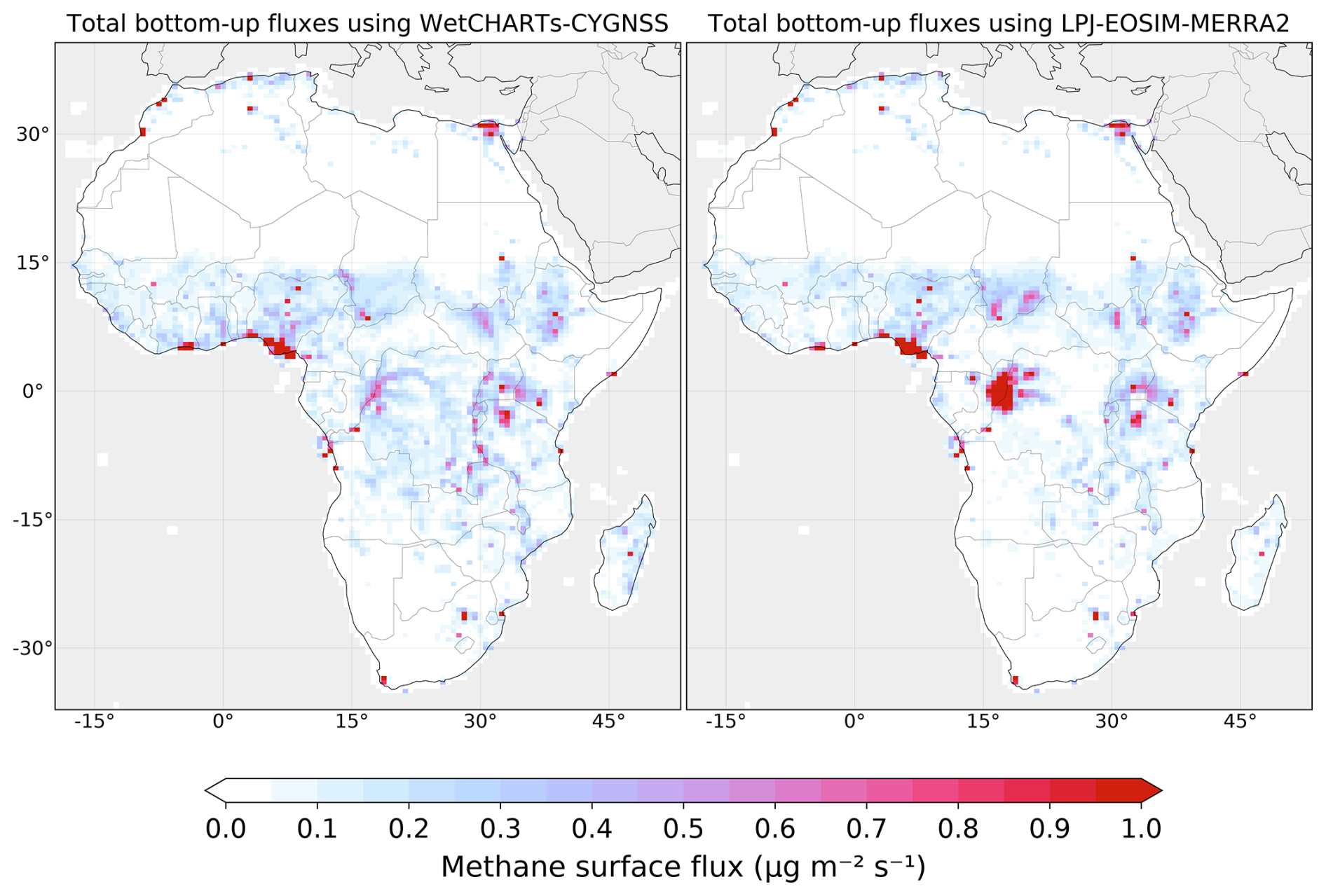
Figure 3 Mean bottom-up methane surface fluxes in 2019–2024 at 0.5° × 0.625° resolution. These fluxes include all sectors in Table 1, differing only in their wetland component, which is either WetCHARTs-CYGNSS (left) or LPJ-EOSIM-MERRA2 (right). Areas in grey are not optimized as part of the state vector (oceans) or are excluded from our analysis (Middle East, southern Europe). Fluxes can be weakly negative (minimum −0.02 µg m⁻² s⁻¹) in remote desert regions due to the soil sink. The colorbar saturates for a few high-emitting grid cells, with the highest emission reaching 5.5 µg m⁻² s⁻¹ in Lagos due to landfills.

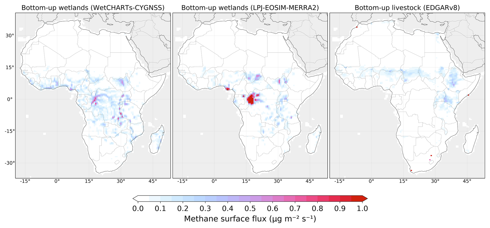
Figure 4 Mean 2019–2024 bottom-up methane surface fluxes for wetlands (WetCHARTs-CYGNSS and LPJ-EOSIM-MERRA2) and livestock (EDGARv8) at 0.5° × 0.625° resolution. LPJ-EOSIM-MERRA2 wetland emissions reach 2.3 µg m⁻² s⁻¹ over the Congo Basin. EDGARv8 livestock emissions reach 2.8 µg m⁻² s⁻¹ in South Africa.

3 African methane surface fluxes

Our optimized 2019–2024 annual mean methane surface fluxes using either of the wetland bottom-up prior estimates are shown in Fig. 5, totaling 71–72 Tg a⁻¹. This range reflects only the uncertainty introduced by varying the prior estimate. Despite using very different bottom-up wetland representations, the two inversions converge to a similar spatial pattern, owing to the ingestion of 6.5 years of TROPOMI observations and our consideration of prior error correlations (Eq. 5) that effectively allow greater departures from the prior estimates in the cost function. The spatial pattern of the optimized fluxes features large emissions from South Sudan, around Lake Chad, and throughout eastern Africa, missing from the prior estimates but consistent with the spatial patterns derived using GOSAT in Lunt et al. (2019). The LPJ-EOSIM-MERRA2 wetland methane emission hotspots in the Congo Basin and southeastern Chad shown in Figs. 3 and 4 vanish in the optimized fluxes.

We validate our results using 10-fold cross-validation as in Turner et al. (2020), in which observations are split into ten subsets and each subset is withheld from the inversion in turn for evaluation. Simulated enhancements with our optimized state vector ($\mathbf{K}\widehat{\mathit{x}}$) show improved performance relative to the bottom-up state vector (Kx_b) when evaluated against TROPOMI-observed enhancements ($\mathit{y}-F(\mathit{x}=\mathrm{0}))$ withheld from the inversion, achieving higher correlation and lower root-mean-square-error (optimized: 0.60 Pearson's r, 8.7 ppb RMSE; bottom-up: 0.49 Pearson's r, 9.4 ppb RMSE). Observations are only withheld from the inversion for the purpose of this cross-validation; all other reported results use all observations.

We disaggregated optimized fluxes to sectors on the basis of relative contributions of individual sectors to the bottom-up estimates in each grid cell, using WetCHARTs-CYGNSS for both inversions as the better bottom-up representation of wetlands. The optimized annual mean surface fluxes of 71–72 Tg a⁻¹ include 28–32 Tg a⁻¹ from wetlands, 23–25 Tg a⁻¹ from livestock, 8.4–9.0 Tg a⁻¹ from waste, and 8.2–9.7 Tg a⁻¹ of soil uptake. The optimized emissions (removing soil uptake) average 80–81 Tg a⁻¹, consistent with the 79–88 Tg a⁻¹ average for 2010–2016 reported in Lunt et al. (2019) for total continental African emissions. As in the bottom-up estimates, wetlands and livestock are the dominant sectors. Optimized oil and gas emissions are 4.1–4.2 Tg a⁻¹, only 60 % of the 6.8 Tg a⁻¹ GFEIv3 estimate, a difference driven by Nigeria and Angola. Recent studies by East et al. (2025) for both countries and Fiehn et al. (2025) for Angola also find this overestimate by GFEI.

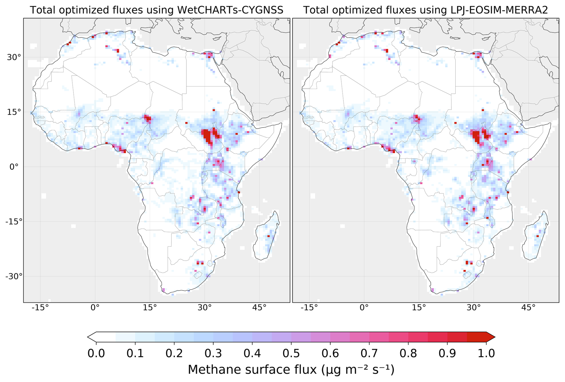
Figure 5 Mean methane surface fluxes in 2019–2024 at 0.5°×0.625° resolution optimized with TROPOMI observations. The two inversions use alternative bottom-up representations of wetlands with WetCHARTs-CYGNSS or LPJ-EOSIM-MERRA2. Emissions reach 3.9 µg m⁻² s⁻¹ in the left panel and 6.5 µg m⁻² s⁻¹ in the right panel, both near the border of Sudan and South Sudan.

4 2019–2024 trends in African methane surface fluxes

The annual surface flux of methane from Africa in each year from 2019 to 2024 is shown in the top panel of Fig. 6. The 7.9–8.6 Tg a⁻¹ increase over 2019–2021 represents 27 % of the 30 Tg a⁻¹ global rise in methane emissions over the same period estimated by He et al. (2025). Although global emissions subsequently decreased back to 2019 levels by 2024 (He et al., 2025), the annual African surface flux continued to increase, up 34 % from 60–62 Tg a⁻¹ in 2019 to 81–82 Tg a⁻¹ in 2024.

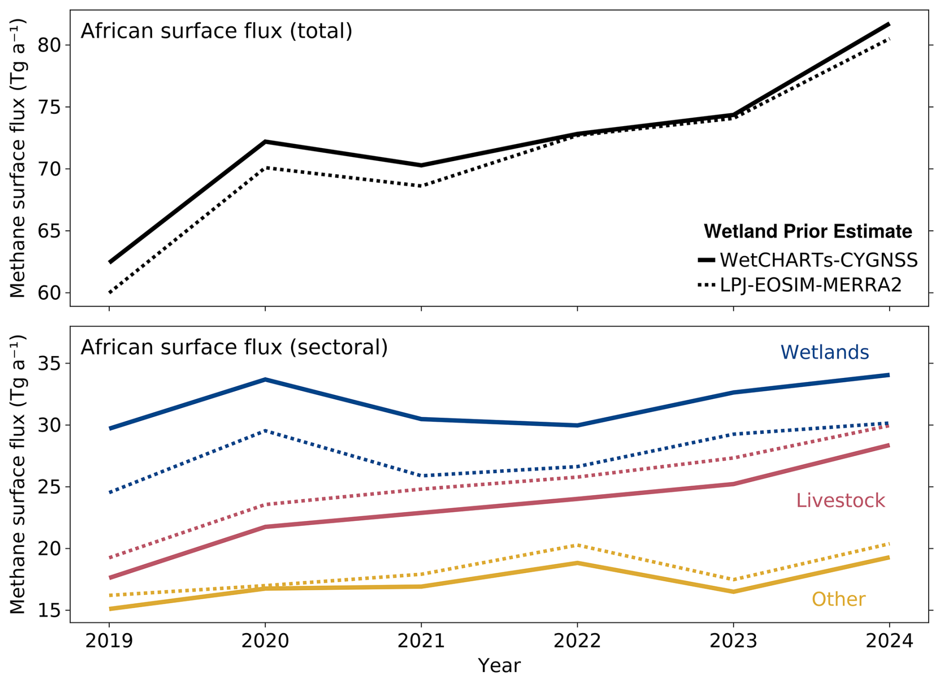
Figure 6 2019–2024 trends in total and sectoral annual mean methane surface fluxes from Africa optimized using TROPOMI. Results are shown for the two inversions using alternative bottom-up representations of wetlands as prior estimates, WetCHARTs-CYNGSS (solid lines) and LPJ-EOSIM-MERRA2 (dotted lines). The sectoral attribution in the bottom panel uses prior spatial information from WetCHARTs-CYGNSS for wetlands. The Livestock category includes enteric fermentation and manure management. The Other category includes waste, fossil fuels, rice, geological seeps, fires, termites, soil uptake, and other minor anthropogenic sources.

The largest increase in the annual African surface flux relative to the previous year was 10 Tg a⁻¹ in 2020. In coarse-resolution global studies using GOSAT and optimizing OH, Feng et al. (2023) found a similar 11 Tg a⁻¹ increase in African emissions from 2019 to 2020, while Qu et al. (2024) reported a 9 Tg a⁻¹ increase. Using TROPOMI and also optimizing OH, He et al. (2025) found an 8 Tg a⁻¹ increase. Consistent with our results, Feng et al. (2023) reported lower emissions in 2021 relative to 2020, though Qu et al. (2024) for 2010–2022 and He et al. (2025) for 2019–2024 report their largest annual African emissions in 2021.

Both of our inversions show that the increase in African methane from 2019 to 2024 was primarily driven by a steady increase in livestock emissions, up 11 Tg a⁻¹ or 60 % in 2024 relative to 2019 as shown in the bottom panel of Fig. 6. Waste emissions increased by 2.5–2.8 Tg a⁻¹ or 37 % over the same period and are mainly responsible for the increase in the Other category in Fig. 6. Wetland emissions increased by 4.3–5.7 Tg a⁻¹ but feature more interannual variability, surging in 2020 and 2024. Previous coarse-resolution inverse studies pointed to the difficulty of separating wetland from livestock emissions in Africa (Pendergrass et al., 2025). We have more confidence in our ability to separate these two sectors because of our higher spatial resolution and monthly temporal resolution, use of more reliable CYGNSS inundation data, and prior error correlations that exploit the broader spatial patterns for each sector.

Figure 7 shows the spatial distribution of the methane surface flux trends for 2019–2024 as derived by the Theil-Sen estimator applied to 72 months of optimized estimates in each grid cell. Results are shown for total fluxes and for the livestock sector. Increasing emissions are mostly in the Sahel, tracking the livestock sector. The hotspot increase in South Sudan is however largely driven by wetlands (mostly the Sudd, but also the Machar and Lotilla wetlands; Pandey et al., 2021). Increases in southeastern Africa are also mostly from wetlands. Oil and gas emissions increase in Algeria but decrease in coastal Nigeria.

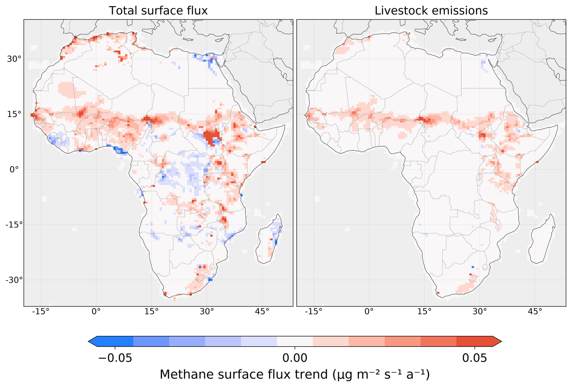
Figure 7 2019–2024 trends in methane surface fluxes from Africa at 0.5° × 0.625° resolution optimized using TROPOMI. Results are shown for the inversion that uses WetCHARTs-CYGNSS as the wetland prior estimate. Trends are obtained by application of the Theil-Sen estimator to the 72 months of surface flux estimates in each grid cell.

The Food and Agriculture Organization (FAO) of the United Nations reports increasing ruminant and pseudo-ruminant livestock populations in Africa over the 2019–2023 period: +28 million cattle, +2.6 million camels, +39 million goats, and +26 million sheep (FAO, 2024). Convolved with Tier 1 emission factors from the IPCC (IPCC, 2019), these livestock population increases (∼ 10 %) correspond to only a 2.4 Tg a⁻¹ increase, well short of the 7.6–8.0 Tg a⁻¹ (40 %) increase in livestock emissions that we infer for 2019–2023. This discrepancy may reflect inaccurate censuses of livestock populations in Africa, which face challenges that include reluctance of farmers to report for taxation or cultural reasons, transhumance, and logistics limitations from civil unrest (Mapitse and Letshwenyo, 2011). For example, Abay et al. (2025) found that directly counted cattle populations were 43 % higher than owner-reported data in Ethiopia, which they attribute in part to incentives for owners to underreport their herd size to maintain social protection program eligibility.

Wetland emissions in central-eastern Africa, including the Congo Basin, Uganda, Zambia, and Tanzania, are elevated in 2020 and 2024 as shown in Fig. 8, correlating with the positive phase of the Indian Ocean Dipole that drives rainfall anomalies in East Africa (Feng et al., 2022; Palmer et al., 2023), and driving the interannual variability of total African emissions (Fig. 6). In contrast, the wetlands of South Sudan, which are the single most prominent wetland methane source in Africa as revealed by our inversion (Fig. 5), have peak emissions in 2022, in line with increased inundation (Hardy et al., 2023; Dong et al., 2024) but out of phase with total African wetland emissions. Rainfall was low in 2022, but the long residence time of water in the White Nile system that connects Lake Victoria to the river-fed Sudd wetlands of South Sudan creates a temporal lag between rainfall and inundation (Mulangwa et al., 2025). Lake Victoria was at its highest level in two decades in 2020 and 2021 because of heavy precipitation (Boergens et al., 2024; Dong et al., 2024).

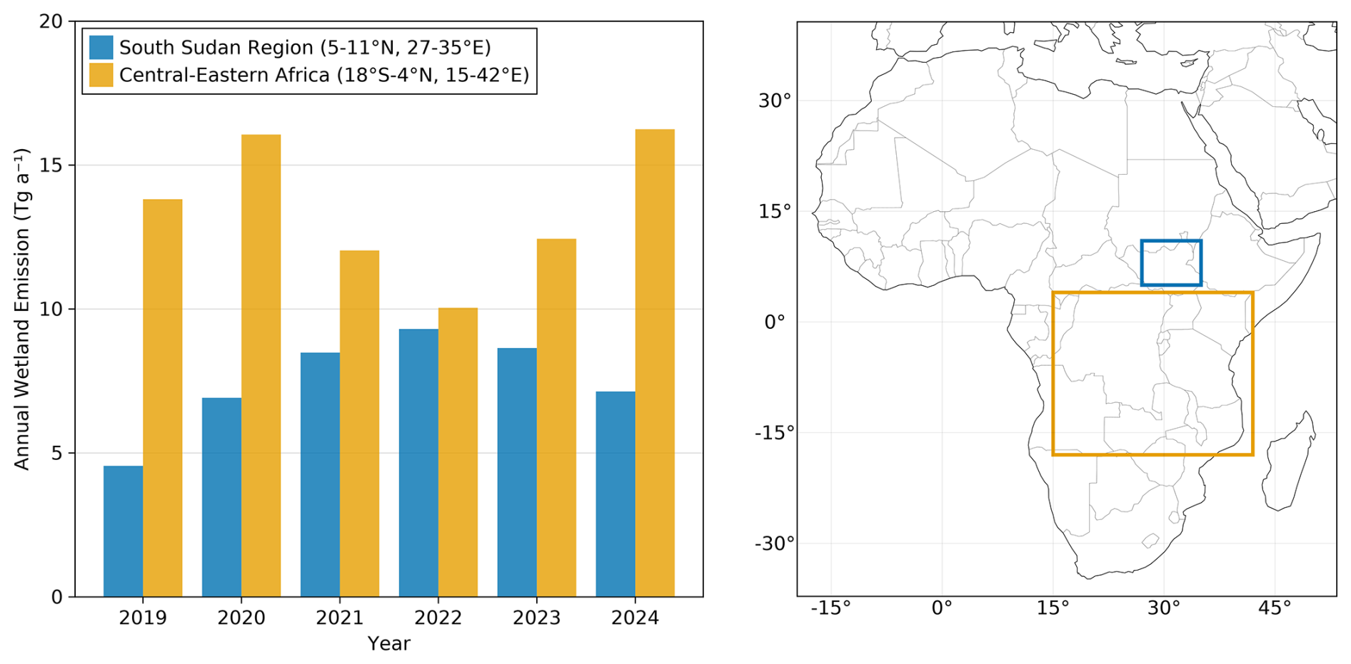
Figure 8 Wetland methane emissions optimized by TROPOMI in the inversion using WetCHARTs-CYGNSS as prior estimate. Annual totals are shown for the South Sudan region and central-eastern Africa.

5 Implications for bottom-up wetland emission models

Our TROPOMI inversion results show that the WetCHARTs-CYGNSS bottom-up model, while performing better than LPJ-EOSIM-MERRA2, still greatly underestimates emissions from South Sudan and Lake Chad and overestimates emissions from the Congo Basin. Uncertainty in bottom-up models for tropical wetlands has been generally attributed to poor inundation data (Pandey et al., 2021; Dong et al., 2024; Lin et al., 2024). However, we find here that the main source of error is in the wetland methane emission intensity (emission per unit inundated area). CYGNSS inundation patterns (Fig. 9) match the pattern of our optimized emissions, but this is corrupted when applying CARDAMOM heterotrophic respiration rates through WetCHARTs to infer the emissions. Figure 9 compares the emission intensities from CARDAMOM to those inferred from our TROPOMI inversion by reference to the CYGNSS inundation data. CARDAMOM broadly tracks photosynthetic uptake, but this appears to be inadequate for estimating methane emissions, producing high intensities in the Congo Basin and low intensities in South Sudan. As a potential alternative to CARDAMOM, also shown in Fig. 9 are methane emission intensities from McNicol et al. (2023), derived from the FLUXNET eddy-covariance flux tower network (Delwiche et al., 2021) by applying machine learning dependences on environmental variables. The strongest dependences in that FLUXNET machine learning product are on temperature. The resulting patterns are opposite of CARDAMOM, with low intensities over the Congo Basin, but still differ greatly from our TROPOMI inversion and do not capture the high intensities in South Sudan. The FLUXNET product includes only two towers in Africa (both in Botswana with data only for 2018, with their site-level intensities ∼ 5× greater than those from our 50 km inversion), so the intensities are derived primarily from observations in other continents.

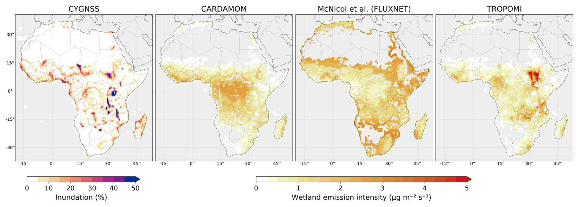
Figure 9 Wetland emission drivers in Africa. Values are 2019–2024 means. The left panel shows the inundated fraction from CYGNSS. The other panels show the methane intensities (emission per unit of inundated area) from CARDAMOM used in WetCHARTs-CYGNSS, McNicol et al. (2023) applying machine learning to FLUXNET tower data (Delwiche et al., 2021), and our TROPOMI inversion referencing optimized wetland emissions to the CYGNSS inundation data. Intensities are only shown for grid cells with average CYGNSS inundation greater than 0.5 %. Wetland emission intensities reach 10.6 µg m⁻² s⁻¹ in the TROPOMI-derived intensity map over the wetlands of South Sudan.

Inspection of the seasonality of emission in South Sudan gives further insight into the shortcomings of the bottom-up wetland emission models. Figure 10 shows monthly optimized wetland emissions for the same South Sudan region as in Fig. 8. Emissions peak in October–November during the short rain season, as previously reported (Lunt et al., 2021). WetCHARTs-CYGNSS has the same seasonality but weaker seasonal amplitude and does not capture the observed interannual variability. LPJ-EOSIM-MERRA2 has near-zero emission in January–March and its seasonal peak is shifted two months ahead of our optimized emissions. Again, CYGNSS inundation alone does much better at reproducing the relative seasonal amplitude and interannual variability in our optimized emissions, but the seasonality is dampened by CARDAMOM which has opposite phase, tracking temperature. CYGNSS inundation peaks one month before our optimized emissions, which may be explained by the time lag for methanogens to activate (Pandey et al., 2021).

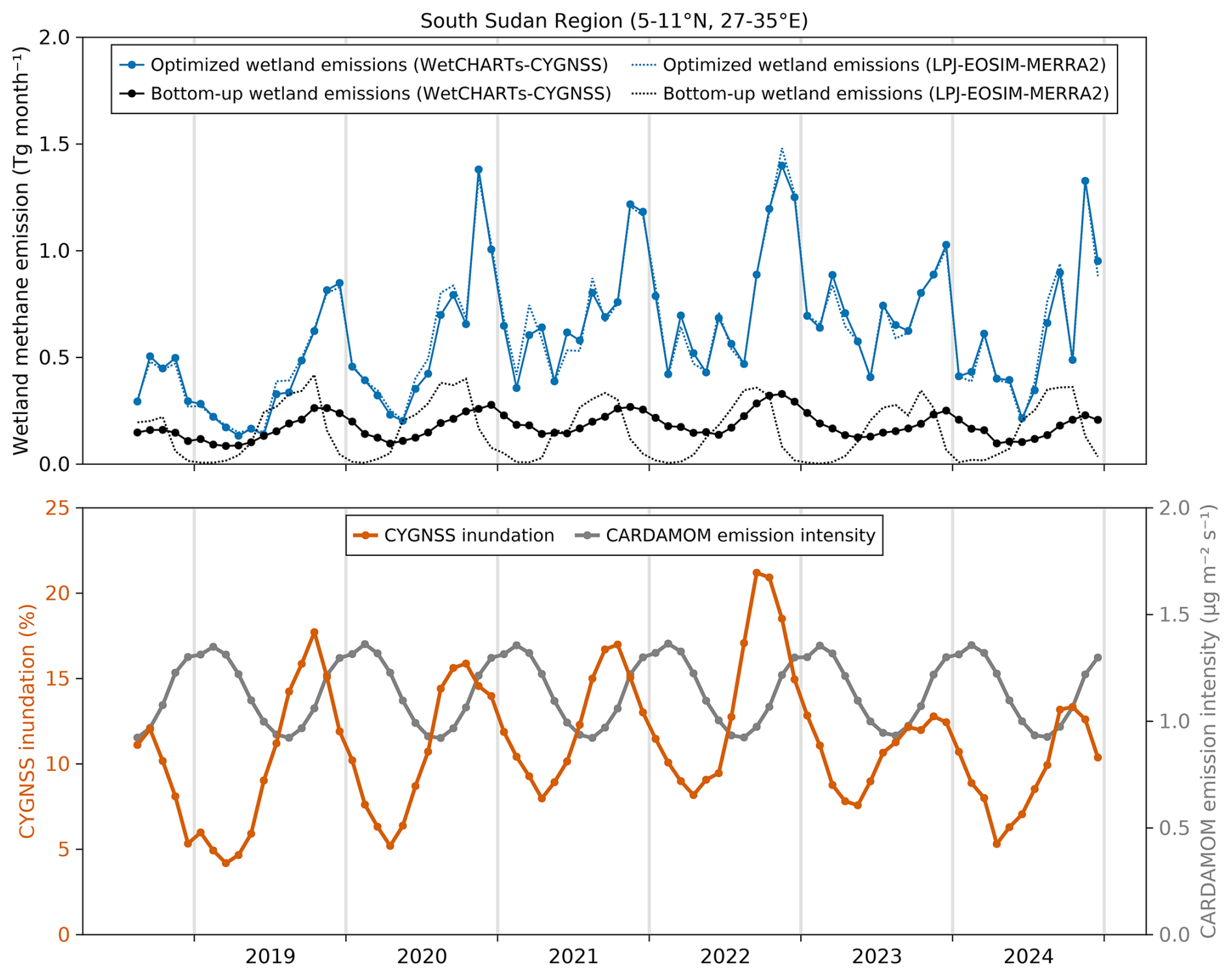
Figure 10 Monthly wetland methane for the South Sudan region (5–11° N, 27–35° E; Fig. 8) over May 2018–December 2024. The top panel shows optimized emissions from our TROPOMI inversions compared to two bottom-up wetland models used as prior estimates, WetCHARTs-CYGNSS and LPJ-EOSIM-MERRA2. The bottom panel shows CYGNSS inundation and CARDAMOM-dervied emission intensities used in WetCHARTs-CYGNSS. Ticks indicate 1 January each year.

6 Conclusions

We used TROPOMI satellite observations of methane in monthly analytical inversions to infer monthly mean methane surface fluxes at 50 km resolution over Africa from August 2018 to December 2024. Our goal was to better understand the role of Africa as a driver of the recent rise in methane and to connect this rise to the underlying emission processes.

Our inversion used a continental-scale nested version of the GEOS-Chem model, with smoothed TROPOMI boundary conditions further optimized by the inversion, to enable high resolution and isolate the effect of African emissions. We constructed bottom-up wetland emissions for use as prior estimates and source attribution with monthly high-resolution inundation data from the CYGNSS satellite constellation in combination with the CARDAMOM biogeochemical model from the WetCHARTs wetland model ensemble (WetCHARTs-CYGNSS). We also used the LPJ-EOSIM-MERRA2 reanalysis-based wetland model as an alternative prior estimate to evaluate uncertainty in our results.

African emissions are dominated by wetlands and livestock. The optimized surface fluxes from our inversion show large changes in spatial distributions relative to the prior estimates, including in particular much higher emissions from the wetlands of South Sudan and much lower emissions from the Congo Basin wetlands. We find little sensitivity of the optimized surface fluxes to the choice of prior estimates, reflecting the large number of observations and our accounting of prior error correlations that effectively decreases the weight of the prior estimates in the inversion. Prior error correlations dependent on spatial similarity in source sectors, as used here, further facilitates the separation of posterior emissions between sectors. This represents significant improvement over the standard practice of assuming uncorrelated prior errors.

We find that the annual African methane surface fluxes increased steadily over the 2019–2024 period, from 60–62 Tg a⁻¹ in 2019 to 81–82 Tg a⁻¹ in 2024 (34 % increase). The 2019–2021 African emissions increase accounts for 27 % of the estimated global growth in methane emissions over that period. However, methane emissions from Africa continued to increase after 2021 even as global emissions decreased back to their 2019 levels. We attribute the 2019–2024 increase in African emissions primarily to livestock (+11 Tg a⁻¹), wetlands (+4.3–5.7 Tg a⁻¹), and waste (+2.5–2.8 Tg a⁻¹). The livestock emissions grew steadily by 60 % over the 2019–2024 period while wetland emissions are more irregular, surging in 2020 and 2024, driven by central-eastern African wetlands. The growth in livestock emissions is mostly in the Sahel. It is much higher than can be explained by the ∼ 10 % increase in livestock populations over the 2019–2023 period reported by the Food and Agriculture Organization (FAO), though the FAO statistics are notoriously uncertain in Africa.

Uncertainty in bottom-up wetland emission estimates has been previously blamed on poor inundation data, but here we find that the CYGNSS monthly inundation maps match closely the spatial and seasonal wetland emission patterns optimized by our inversion. Our results suggest that the main shortcoming in bottom-up wetland emission models is in the estimate of methane emission intensity per unit of inundated area. CARDAMOM used by WetCHARTs relates this intensity to heterotrophic respiration, but this appears to be incorrect and is responsible for the large overestimate in the Congo Basin. McNicol et al. (2023) derive methane intensities from FLUXNET tower data as primarily driven by temperature, which corrects the Congo Basin but fails to capture the high emissions in South Sudan. More work is needed to estimate methane emission intensities in bottom-up wetland emission models, and the intensities derived from our TROPOMI inversion may provide guidance for this purpose.