Evaluating simulations of ship tracks in a km-scale model

Clouds, and in particular their adjustments following an aerosol perturbation, remain a major source of uncertainty in climate projections, due to the wide range of scales over which cloud processes act on. This uncertainty limits our capability to simulate potential solar radiation management strategies, such as marine cloud brightening (MCB). A “natural”, or “opportunistic”, experiment for investigating MCB is analysis of ship tracks, as they mimic the intended effect and allow us to investigate time evolving cloud adjustments. In this study, we model a real case of ship tracks and evaluate model performance in representing the lifetime of cloud adjustments through comparisons with satellite observations. Requiring accuracy in individual cases creates a particularly challenging test for simulations of aerosol-cloud interactions, but it is necessary to ascertain whether this model is suitable for simulating MCB accurately.

Our findings highlight a key deficiency in activation parameterisations when simulating high aerosol number concentrations – such as those expected in MCB scenarios. While the model can replicate the mean cloud properties within ship tracks, it struggles to capture the temporal evolution of the adjustments. Specifically, in precipitating clouds, both the enhancement in droplet number concentration (N_d) and subsequent adjustment to liquid water path (LWP) are overestimated and persist for too long. This discrepancy between model and observations is linked to excessive model sensitivity to N_d perturbations in precipitating conditions, leading to unrealistically strong suppression of drizzle, and ultimately resulting in simulated ship tracks which overestimate the cooling effect in these cases. We identify scenarios in which current formulations of parameterisations are not suitable for use in simulating high-concentration aerosol perturbations, such as MCB, and scenarios in which models are more capable.

1 Introduction

A large portion of the uncertainty in estimates of the effective radiative forcing from aerosol-cloud interactions originates from poor model representation of clouds (Smith et al., 2020), and our understanding of how clouds adjust following an aerosol perturbation. Clouds depend on processes operating at micron scales, rendering their explicit representation unfeasible in most computationally viable resolutions of weather or climate models. Consequently, cloud processes must be parametrised. These parameterisations define the process rates, which describe how much physical properties change between each model time step. Uncertainty in these parameterisations leads to considerable uncertainty in model estimates of the radiative forcing from aerosol-cloud interactions, with a large portion of this uncertainty stemming from the amount of liquid cloud (Zelinka et al., 2014). Addressing and reducing this uncertainty is crucial for enhancing the accuracy of future climate projections (Andreae et al., 2005). Better representation of clouds in regional weather forecasting models would improve predictability of clouds and the onset of precipitation (Field et al., 2023). This uncertainty is also important for marine cloud brightening (MCB), a proposed solar radiation modification (SRM) strategy aimed at reflecting more sunlight by intentionally seeding clouds with aerosols (Diamond et al., 2022; Wood, 2021; Salter et al., 2008; Zhang and Feingold, 2023). Uncertainty in model representation of high-concentration aerosol-cloud processes limits our capability to simulate MCB experiments, and makes the design of suitable field trials difficult.

To assess the longer term impacts of MCB on our climate, it must be incorporated into climate model simulations. One suggested approach involves the use of regional models to accurately simulate the localised effects of MCB, and use this to parametrise its impact in coarser resolution global climate models (Feingold et al., 2024). This is a particularly challenging task for climate models. While recent models are able to adequately simulate patterns of cloudiness (Tselioudis et al., 2021), their simulation of aerosol-cloud interactions is more varied (Gryspeerdt et al., 2020). However, these evaluations are typically done on large-scale temporal or spatial averages – assessments of MCB efficacy require accurate simulations of the model response to individual clouds. This is not well evaluated by current techniques. In addition, as many of the same parameterisations for cloud microphysics are used across both coarse and finer resolution models (e.g. activation and precipitation processes), greater confidence in our regional representation of MCB should inform our global modelling capability, avoiding the equifinality problem in larger-scale studies (Mülmenstädt and Feingold, 2018). Robust evaluation frameworks are needed to assess the realism of regional models, not only in terms of short-wave (SW) radiative forcing but also with respect to the representation of key processes.

Ship tracks, the narrow cloud features formed by aerosol emissions from ships, offer a valuable “natural experiment” for studying the interactions that would occur in intentional MCB (Christensen et al., 2022; Diamond et al., 2022). Aerosols in the ship plume act as cloud condensation nuclei, causing the cloud to have more, smaller, droplets which reflect more incoming solar radiation. This is known as the “Twomey” effect, and is well documented on short timescales (Twomey, 1974, 1977; Ferek et al., 1998; Hobbs et al., 2000; Ackerman et al., 2000; Feingold et al., 2003; Penner et al., 2004; Segrin et al., 2007; Christensen et al., 2022). The brightening observed in ship tracks mimics the intended effect of MCB, offering a real-world analogue for testing the feasibility of such interventions. Ship track studies provide information about aerosol-cloud interactions in this marine context, and can be useful in assessing the behaviour of models that are intended for use in simulating MCB.

After the initial droplet number (N_d) perturbation, clouds respond to aerosol perturbations over longer timescales through effects known as “cloud adjustments”. A precipitation suppression effect (Albrecht, 1989; Rosenfeld, 2000), where smaller cloud droplets take longer to form precipitation, increasing liquid water path (LWP), tends to result in additional cooling. Alternatively, smaller droplets can also enhance the mixing of dry air above cloud-top into the cloud (a process known as entrainment) and reduce LWP, resulting in a warming effect (Ackerman et al., 2004; Bretherton et al., 2007). This bidirectional response in the LWP can depend on the initial conditions of the unperturbed cloud (Han et al., 2002; Ackerman et al., 2004; Michibata et al., 2016; Toll et al., 2017, 2019; Gryspeerdt et al., 2019a; Possner et al., 2020; Glassmeier et al., 2021; Zhang et al., 2022; Fons et al., 2023), whilst also being controlled by covarying meteorology (Goren et al., 2025).

There is considerable uncertainty in both the sign and magnitude of adjustments (Glassmeier et al., 2021), which is relevant for MCB purposes, since adjustments involving decreasing the LWP could offset the intended cooling impact. Part of this uncertainty stems from both the difficulty in making observations of aerosol-cloud processes, and isolating the impact of aerosol from background meteorology (Christensen et al., 2022). Cloud adjustments are inherently time-dependent processes (Gryspeerdt et al., 2021), yet many observational studies do not consider the time evolution of a cloud response, making it difficult to observe the processes occurring. This limits our modelling capability of these interactions, since without time-resolved observations, it is difficult to capture the time dependence for instantaneous/short timescale injections (such as from ship aerosols or MCB).

Simulating ship tracks provides an opportunity to simulate the intended effects of MCB, and evaluate a model's ability to represent the cloud response to an aerosol perturbation realistically. By simulating ship tracks we can disentangle aerosol effects from meteorological variability because the aerosol source is known and relatively localised. This is possible since we can use the region neighbouring the ship track as an unperturbed “control” region (Segrin et al., 2007), which is a proxy for what the cloud would have looked like if no ship was there. Ship tracks are therefore ideal for isolating the causal impact of aerosols on cloud properties and separate meteorological co-variations (Goren et al., 2025). Additionally, we can view ship tracks as linear formations of independently perturbed clouds (Kabatas et al., 2013), thereby allowing us to infer information about the time evolution of the aerosol perturbation (Gryspeerdt et al., 2021). This helps us evaluate model process representation, such as the activation of cloud droplets (which occurs on the order of seconds to minutes; Arabas and Shima, 2017), or the autoconversion of cloud droplets into rain droplets (occurring on longer timescales, on the order of minutes to hours; Stephens and Haynes, 2007).

In order to answer questions relating to MCB experimental design, accurate simulations of ship tracks are vital, however we must be certain that model simulations produce the correct answer for the right reasons. This calls for in depth evaluation of the representation of model processes, not just the final forcings – ship tracks provide an avenue to do this. Simulating MCB provides an exceptionally challenging task for the field, since accuracy is not only required in terms of large-scale/domain-wide averages, but instead at the scale of individual cloud perturbations.

Previous efforts have been made to simulate ship tracks in atmospheric models, in order to assess model performance (Wang and Feingold, 2009; Possner et al., 2015, 2018; Berner et al., 2015; Chun et al., 2023). Berner et al. (2015) and Wang and Feingold (2009) utilise fine resolution LES models to investigate the effect of aerosol perturbations on marine stratocumulus, but cannot make direct comparisons to observations since they are not real cases of ship tracks. Similarly, McMichael et al. (2024, 2025) investigate ship track spreading rates with LES, and Prabhakaran et al. (2024) use LES to investigate impacts on the stratocumulus-to-cumulus transition. Possner et al. (2015) use observations of a real case of ship tracks, yet the simulated ship locations are not from the actual ships that caused the observed ship tracks, which limits the ability to assess the accuracy of MCB simulations. Additionally, whilst previous studies have typically attempted to quantify the N_d response, relatively few have sought to investigate the simulated representation of the LWP adjustment.

In this work, we produce simulations of a real case of ship tracks, using ship emissions locations from ship Automatic Identification System (AIS) data. We utilise a double-moment cloud microphysics scheme – Cloud AeroSol Interacting Microphysics (CASIM; Field et al., 2023) in the Met Office Unified Model (UM) in regional configuration (allowing for convection to be resolved), and compare directly to satellite observations. We simulate changes in cloud properties (N_d and LWP), investigating the processes involved as well as the time evolution of the response. This allows us to evaluate the model representation of the cloud adjustments to a N_d perturbation. Crucially, we do not investigate the model representation of the aerosol microphysics, and are more concerned with the subsequent cloud adjustments after an initial N_d perturbation is applied. We evaluate our simulations according to the three criteria described in Sect. 2.1, in order to ensure the proper change in cloud radiative effect is captured via the correct microphysical processes. In order to properly simulate MCB impacts we must simulate the correct behaviour, and for the correct reasons.

Through evaluating our simulated ship tracks against these criteria, we reveal issues in current model representation of the activation of cloud droplets at high aerosol number concentrations, and lifetime of the LWP adjustment. We identify scenarios in which current formulations are more suitable for simulating MCB, and scenarios in which further work is needed before models can be considered credible. Furthermore, we make suggestions on experimental design, such that analysis and quantification of the N_d and LWP perturbations are least uncertain.

2 Methods

2.1 Criteria for evaluating ship tracks

In order to evaluate the model simulations of individual ship tracks, rather than a larger-scale temporal or spatially aggregated assessment, we define the following criteria.

1. Accurate representation of changes in CRE. The cloud radiative effect (CRE) in overcast scenes is largely dependent on the inside ship track N_d and LWP values (Possner et al., 2015), which encapsulate both the Twomey brightening and subsequent LWP adjustments. We want to ensure our model is producing simulations with the correct numerical values inside the ship track. Due to difficulties in obtaining perfect background simulations, our first criteria considers solely the absolute values where the ship perturbation has been applied, since this is ultimately where it is key to get the behaviour correct.

2. Accurate time evolution of the CRE. This criteria enables us to evaluate the lifetime of the ship effect and therefore the associated radiative forcing. Again, this effect is driven by changes in LWP and N_d. The model sensitivity to and aerosol perturbation can be evaluated, as the enhancement from the unperturbed (control) state is taken into account. Ship tracks provide a method for obtaining time evolution even in snapshot satellite imagery (Gryspeerdt et al., 2021), therefore information about the time-evolution of the cloud response can be made.

3. Sensitivity in the N_d response to initial conditions. Previous studies have shown that the cloud response is sensitive to the initial conditions of the cloud (Ackerman et al., 2004; Michibata et al., 2016; Toll et al., 2017, 2019; Gryspeerdt et al., 2019a; Possner et al., 2020; Glassmeier et al., 2021; Zhang et al., 2022; Fons et al., 2023). In order for our model representation of clouds to be accurate this sensitivity must be reflected in the model. We expect to see different responses in precipitating and non-precipitating conditions, and this is investigated in our model simulations. In order for the model to reproduce the correct response for the right reasons, this dependence on the initial cloud conditions should be satisfied. This should confirm that the model is sensitive to the correct model processes.

We apply the above criteria by considering temporal evolutions (treating the length of a ship track as a time since aerosol injection axis) of inside track N_d and LWP, and the associated enhancements from the background (the calculation of which is explained in Sect. 2.6). We discuss the “correctness” with respect to each criterion in terms of the similarities and differences between the observed responses compared to the simulated responses.

2.2 Model configuration

Our case study is simulated using the Met Office Unified Model (UM, version 13.0; Brown et al., 2012), in the Regional Atmosphere and Land (RAL) configuration 3.1 (Bush et al., 2020, 2023, 2025). Our domain covers the Eastern and Central Pacific, off the coast of California (Fig. 1). The 2625 km by 1125 km domain is centred on (40° N, 135.25° W) with a horizontal resolution of 1.5 km. There are 90 levels up to 40 km, with 16 levels below 1 km. The model time step is 75 s, and the lateral boundary conditions to the nested regional model are provided hourly by the UM global model at N216 resolution (≈ 60 km) in Global Atmosphere (GA) 6.1 science configuration (Walters et al., 2017). Our simulations are initialised from global model analysis at 00:00Z on 11 July 2018 and run for 48 h.

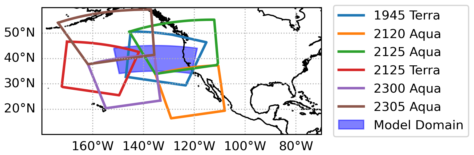
Figure 1 Granules from Aqua and Terra overpasses on 12 July 2018 that intersect with the model domain of this study.

To properly simulate the cloud adjustments to an aerosol perturbation in a cloud resolving model, a double moment cloud microphysics scheme is recommended (Morrison et al., 2009; Igel et al., 2015). Double-moment microphysics schemes prognose both the mass and number concentration of each hydrometeor species (e.g. Ferrier, 1994; Seifert and Beheng, 2006). A double-moment microphysics scheme allows N_d to be recalculated at each time step, and therefore can subsequently modify process rates (such as autoconversion), impacting the cloud evolution over time (Field et al., 2023). In single moment schemes, the number concentration of each species (from which the process rates are derived) are either constant or diagnosed from other meteorological parameters using empirical relationships. These schemes, whilst computationally cheaper, can fail to accurately represent the indirect effect from aerosol-cloud interactions (Gordon et al., 2020).

For cloud microphysics, we employ the Cloud AeroSol Interacting Microphysics (CASIM) scheme (Shipway and Hill, 2012; Field et al., 2023). CASIM is a double moment scheme with five hydrometeor species (cloud liquid, rain, ice, snow, and graupel) in which both mass and number concentration mixing ratios are prognosed. Each cloud species' particle size distribution (PSD) is described using a generalised gamma function with constant shape parameters. The autoconversion of cloud droplets into rain droplets and accretion of cloud water by rain are parametrised in CASIM following Khairoutdinov and Kogan (2000). CASIM also contains other warm cloud processes, such as aggregation (rain collecting rain), and we refer the reader to Field et al. (2023) for details on these parametrised processes.

We couple CASIM to the double moment modal Global Model of Aerosol Processes aerosol microphysics scheme (GLOMAP-mode; Mann et al., 2010), within United Kingdom Chemistry and Aerosols (UKCA) sub-model, where aerosols are represented by five log-normal modes. These are the nucleation, Aitken, accumulation, coarse, and “Aitken insoluble” modes. Both the number and mass of each of the four chemical components (sulphate, sea salt, black carbon, and organic carbon) are prognosed in this double moment scheme. Black carbon cannot enter the nucleation mode, and sea salt cannot enter either the nucleation or Aitken modes. Dust is represented separately within the CLASSIC binned sectional scheme (Woodward, 2001). GLOMAP-mode simulates aerosol microphysical processes such as the nucleation of new particles, coagulation of particles, condensation, and cloud processing (Mann et al., 2010). Particles can grow through condensational growth or coagulation between particles, and is represented by an increase in particle diameter, which can move particles into a greater size mode. Particles in soluble modes can also absorb atmospheric water and undergo hygroscopic growth (Yoshioka et al., 2025).

Coupling between GLOMAP-mode and CASIM allows for aerosol mass and number concentrations of the Aitken, accumulation, and coarse aerosol modes to be passed into the CASIM activation scheme for the production cloud droplets (Gordon et al., 2020), which is parametrised by Abdul-Razzak and Ghan (2000, ARG). Autoconversion and accretion rates from CASIM are summed and passed back into GLOMAP-mode to calculate the removal of aerosol (that are inside droplets) by rain. Rain rates also determine the removal of aerosol through impaction scavenging. GLOMAP-mode also uses the liquid water content from CASIM to calculate the rate of conversion of sulphur dioxide into sulphate inside cloud droplets (Gordon et al., 2020).

Our simulations are coupled to the standard radiative transfer scheme in the UM (using the RADAER module; Bellouin et al., 2013) in order to calculate the aerosol radiative effects, however the direct radiative effect of aerosols from shipping is not the main focus of this study.

Within our simulations, we only consider aerosol in the soluble accumulation mode and initialise our simulation with a constant sulphate aerosol number concentration of 200 cm⁻³, characteristic mass 3 × 10⁻¹⁸ kg, and aerosol diameter of ≈ 0.1 µm, which is typical of sulphate aerosols (Noone et al., 2000). Aerosol is allowed to evolve freely after the model simulation begins, with the boundaries determined by the global driving model. As described in Gordon et al. (2020), aerosol mass and number concentrations can vary as determined by the microphysical processes in GLOMAP-mode, however CASIM does not have the capability to track aerosol tracers within hydrometeors and therefore cloud microphysics does not alter aerosol mass/size/composition except through irreversible removal via wet-scavenging.

Whilst we only consider our initial aerosol field to be in the accumulation mode, there are still background emissions into other modes. The different types of non-ship aerosol sources are described in Mann et al. (2010), with emissions from marine phytoplankton, SO₂ from volcanoes, fires, and industrial sources. In the simulations of our study, we use anthropogenic emissions from the Coupled Model Intercomparison Project (CMIP6) inventory (Feng et al., 2020). The emissions are at a low resolution of ≈ 135 km (Gordon et al., 2023). Natural emissions of sea salt, primary marine organic aerosol, and dust are parameterised as described in Mulcahy et al. (2020) and Gordon et al. (2020). The emissions of sea spray, sulphate and carbonaceous aerosols are allocated to modes according to their size distribution (Mulcahy et al., 2020), whereas biofuel, fossil fuel, and biomass burning emissions are emitted into the Aitken insoluble mode and then undergo “ageing” (Mann et al., 2010) into the Aitken mode in certain conditions. Secondary organic aerosol (SOA) are produced from the oxidation of monoterpenes (Mulcahy et al., 2020). Further details on other trace gas and aerosol emissions within this regional model set up are described in Gordon et al. (2023). These emissions can enter different aerosol size modes, not just the accumulation mode that the simulation is initialised from, however it is the accumulation mode aerosol mass/number concentrations that will dominate.

This assumption whereby we initialise our aerosol fields only in the soluble accumulation mode enables us to consider differences between control and ships runs as solely a function of increasing aerosol number concentration at the ship location, and the effects of aerosol chemistry are neglected. Differences in hydroscopicities in other aerosol-modes are assumed to be a less important factor in droplet activation than the mass/diameter of the mode (Dusek et al., 2006). A similar initialisation from a uniform aerosol field of accumulation mode aerosol has been conducted before in Grosvenor et al. (2017), and was found to produce N_d that were in approximate agreement with observations. However, this assumption is evidently a significant simplification to our aerosol configuration, as the accumulation mode will dominate the aerosol mass and number concentrations, with the concentrations of other modes only impacted by the natural and anthropogenic emissions described above. We discuss the potential consequences of this in Sect. 4.1.2.

As a result of this simplified aerosol configuration, our only discussion of aerosol-microphysics concerns how the order of magnitude of the injected ship aerosol influences the activation scheme, and relies mainly on offline calculations. Subsequent investigations therefore consider only the model's representation of cloud adjustments to a droplet number perturbation, without evaluating aerosol microphysics or aerosol realism. Future work that increases the level of complexity and considers aerosol properties through to cloud adjustments within more realistic aerosol configurations would be valuable. Nevertheless, this study is intended as a first step toward understanding model representation of cloud adjustments within ship tracks in this context.

2.3 Simulating ship tracks

In order to simulate the shipping impacts on clouds, we add five ships to our simulation in our ships run. We use container ship locations identified in AIS data and matched to observed ship tracks from 11–12 July 2018, to add realistic moving sources of aerosol (Smith et al., 2015). Details of ship start/end positions and velocities can be found in Table 1. Container ships are selected because of their large size and high emissions, meaning that the resulting ship tracks are the most distinct in the observations. Our five selected ships also cover both directions of the shipping route within the domain. Aerosol is added in a model level at 10 m above sea level and immediately dispersed throughout the 1.5 km by 1.5 km grid box using the following equation:

$$\begin{array}{}\text{(1)}& N_{x,y,z,t+\mathrm{1}}=N_{x,y,z,t}+{\displaystyle \frac{\mathrm{d}N}{\mathrm{d}t}}\times {\displaystyle \frac{\mathrm{\Delta }t}{V}}\end{array}$$

where $\frac{\mathrm{d}N}{\mathrm{d}t}$ is the rate of production number (the rate of ship aerosol emissions) in s⁻¹, Δt is the model time step (75 s), and V is the grid box volume. This describes the aerosol number concentration added to the entire grid box per time step. At this model resolution, ship tracks form at a minimum width of 1.5 km. Typical ship tracks have a width of on the order of 10 km (Durkee et al., 2000), therefore this model resolution is suitable to capture the horizontal extent. Aerosol is almost immediately transported up to cloud base, and there is little deposition of aerosol at the bottom model level, therefore the 10 m injection height (whilst an underestimation) is approximately correct.

Table 1 Start and end locations of 5 container ships, with associated velocities, emission rates. Ships are initialised at 00:00Z 11 July 2018, and allowed to travel for the 48 h of the simulation.

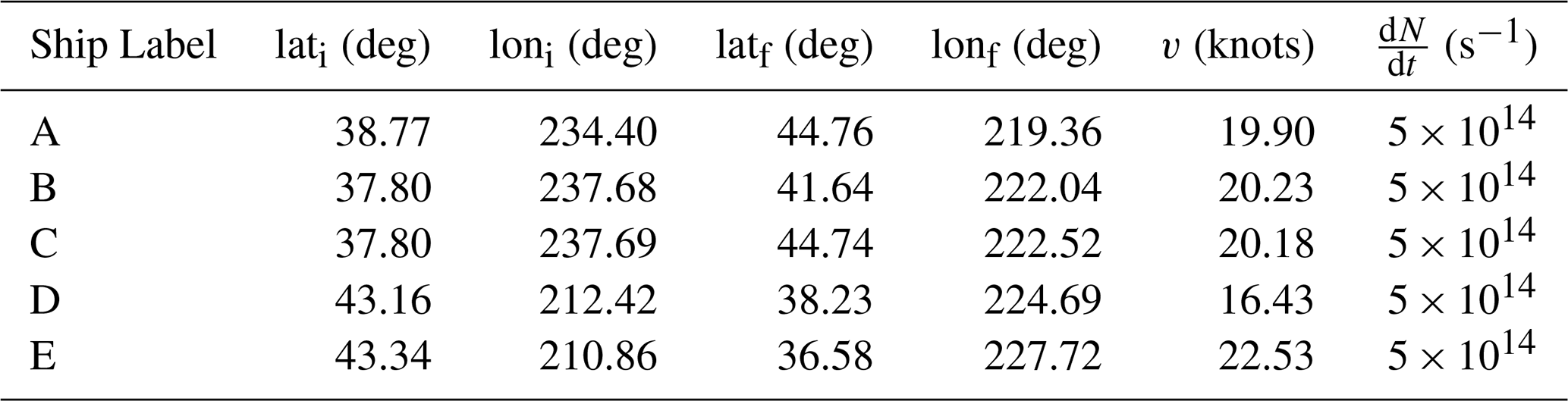
Realistic emissions of condensation nuclei (CN) from ships fall in the range 10¹⁶ to 10¹⁸ kg s⁻¹ (Taylor and Ackerman, 1999; Hobbs et al., 2000; Berner et al., 2015). Connolly et al. (2014) find that the ARG activation parameterisation (Abdul-Razzak and Ghan, 2000) exhibits a sharp “drop off” in activated fraction at increasing aerosol number concentrations (albeit, for NaCl), therefore we investigate the use of a high ship aerosol case (ship production number 10¹⁶) and a lower ship aerosol case (ship production number 5 × 10¹⁴) in this study (Sect. 3.1). We add the aerosol into the accumulation soluble mode with a mass 3 × 10⁻¹⁸ kg, the same as background aerosol, meaning that both our background and ship aerosols are only in the accumulation mode with the same mass. This is done to simplify simulations and isolate causal cloud adjustments in our analysis, since differences between the ships and control run can be attributed to the increased aerosol number concentration at the ship locations. Since these are not the actual emissions from the real ships, there is a considerable source of uncertainty introduced by this “best guess” of the emissions. However, since in this study we are not investigating the model representation of aerosol microphysics and instead are concerned with the model representation of the cloud adjustment to changes in N_d, this estimation of the emissions is deemed reasonable.

2.4 Satellite data

To evaluate our model simulations, we use observations from NASA's Aqua and Terra satellites to compare to our model output. We use Level-2 Collection 6.1 data from the Moderate Resolution Imaging Spectroradiometer (MODIS; Platnick et al., 2017) to obtain LWP and derive N_d following Quaas et al. (2006).

We collocate Aqua and Terra overpasses the occur during our simulation with our model domain, and only consider images the contain any part of a ship track, obtaining six snapshots of our domain, as shown in Fig. 1. Model data is output hourly, therefore we compare satellite data to model output from the nearest time step. When model data is compared to satellite data, the model output is masked only to consider the region contained within the associated satellite snapshot.

Simulated precipitation in the domain is evaluated against ERA5 surface precipitation (Hersbach et al., 2020), as well as Global Precipitation Measurement (GPM-IMERG; Huffman et al., 2014) and overpasses from the Cloud Profiling Radar (CPR) onboard CloudSat (both the 2C-Precip-Column and 2C-Rain-Profile products; Stephens et al., 2008; Haynes et al., 2009; L'Ecuyer and Stephens, 2002). We investigate the probability of precipitation across N_d – LWP space using observations from the CCCM (CERES–CloudSat–CALIPSO–MODIS) combined product (Kato et al., 2010, 2011). We use the CloudSat CPR precipitation flag (from 2C-Precip-Column; Haynes et al., 2009) to define a probability of precipitation as counts of liquid precipitation or drizzle divided by all counts, per N_d-LWP bin (from MODIS Aqua). Since in 2018 CloudSat was not part of the A-train (and therefore not collocated with MODIS), we use observations from 2007–2011, as in Gryspeerdt et al. (2022).

2.5 Ship track locations

We follow a methodology similar to that of Tippett et al. (2024), Gryspeerdt et al. (2021), and Manshausen et al. (2022) to obtain our ship track locations. Using ship positions (from AIS data) we infer the locations of clouds which experienced an aerosol perturbation (neglecting the time taken for aerosol to reach cloud base). These positions are advected in wind fields over time to predict ship tracks which consist of not only location, but the associated time since that location experienced the aerosol perturbation. This allows the length of a ship track to be treated as a time axis, and discern time evolution after an aerosol perturbation even in snapshot imagery (Kabatas et al., 2013).

In our observations of ship tracks in this case study, the hourly ship locations are advected in ERA5 reanalysis winds at 0.25° resolution and 3 h intervals (Hersbach et al., 2020) between the surface and the boundary layer top, with vertical motion within the ship plume following Briggs (1965) (see Tippett et al., 2024 for further details). In model output, the same ship locations are advected instead in the model winds following the same methodology.

Since this study is comparing only five ship tracks between model output and satellite data, it is essential that the exact ship track location is logged as to properly quantify the aerosol effects. We apply small corrections to our model and satellite output track locations from the above methodology to ensure that our track location falls exactly on each visible ship track, for both model output and observations. This is done by hand logging the nearest point of the visible track, perpendicular to the predicted track location. This is not possible in large composite studies which contain thousands of ship tracks, however due to the small number of ships considered in this study it is feasible, and ensures the most accurate measurement of the cloud responses.

Following Tippett et al. (2024), we regrid our datasets to 2D space for each ship track, at each model time step/MODIS snapshot. This 2D space consists of the “time along track” (binned to 1 hourly windows), and the perpendicular “distance away from track” (binned to 1 km). This allows us to investigate exactly how the cloud properties vary with time since aerosol perturbation and distance from the centre of the perturbation.

2.6 Quantifying enhancements

A key challenge in this study is determining the most appropriate method for quantifying the impact of ship emissions on clouds across our two datasets: model simulations and satellite observations.

For the UM-CASIM simulations, the impact of ship-emitted aerosols can be directly quantified by comparing the enhancement in cloud properties between the ships run and the control run. To mitigate stochastic noise between model runs, we apply Gaussian smoothing to the model fields (smoothing with a Gaussian kernel with standard deviation of 0.75 km) before calculating the percentage difference to obtain enhancements in N_d and LWP (ϵ_N and ϵ_L). This approach allows for an estimation of aerosol-induced changes while minimising the influence of small-scale variability in between model runs.

In contrast, defining a control region in observational data is less straightforward (Christensen et al., 2022). Traditional observational studies of ship tracks typically identify an “unpolluted” reference region located approximately 30 km perpendicular to the ship track (Manshausen et al., 2022). This region serves as a control from which the percentage enhancement in cloud properties is calculated. However, this methodology presents potential biases. Specifically, non-linear background gradients can introduce systematic errors in the estimated aerosol effect (Tippett et al., 2024). Additionally, in scenes containing multiple ship tracks, this approach becomes increasingly uncertain. For instance, in our case study, many “outside track” regions that are used as controls inadvertently overlap with other ship tracks. Consequently, the percentage enhancement derived from such comparisons likely underestimates the true aerosol impact (Yuan et al., 2025). Despite these limitations, this method remains the most viable approach given the constraints of observational data.

In Fig. 8j, l we compare the use of (a) the control simulation and (b) the “outside” region to define the unperturbed cloud for the model simulation (solid orange and dashed orange lines, respectively). For the model, we find that both methods for calculating model enhancements produce the same results (to within 15 % and 10 % for N_d and LWP enhancements in the first 15 h of ship tracks, respectively). Our model background has little background variability, and any variability is much smaller than the large perturbation inside the ship track, therefore both methods provide similar results. This would not necessarily be the case in a model simulation with greater background variability.

2.7 Expected enhancements

Using Eq. (1) from Gryspeerdt et al. (2019b), we can calculate expected enhancements in cloud droplet number concentration (ϵ_N) based on the background N_d as a function of aerosol mass emission rates

$$\begin{array}{}\text{(2)}& {\mathit{ϵ}}_N={\displaystyle \frac{M_{\mathrm{E}}^{\mathit{\gamma }}}{\mathit{\alpha }+\mathit{\beta }{N}_{\mathrm{cln}}}}+\mathrm{1}\end{array}$$

where M_E is the mass emission rate (in kg s⁻¹), N_cln is the unperturbed background N_d, and the constants α, β, and γ are 0.1041, 0.0038 and 0.36 as obtained from the fit in Gryspeerdt et al. (2019b). This equation provides a useful method of evaluating whether or not our model is producing enhancements of the right order of magnitude, based on its background conditions.

3 Results

3.1 Activation of aerosol

Using Eq. (1), and a realistic ship production number of 10¹⁶ s⁻¹, we obtain aerosol number concentrations within the ship track of roughly 20 000 cm⁻³. This is realistic given in-situ observations of ship tracks (Hobbs et al., 2000; Noone et al., 2000). However, with these values, our simulated ship tracks exhibit bizarre “split” behaviour, with no cloud droplets activated inside the centre of the track where the aerosol number concentrations are highest (see Fig. 2).

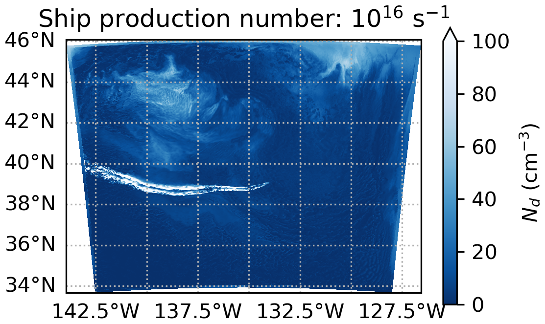
Figure 2 Example of how realistic ship emissions (10¹⁶) produce a “split” ship track due to non-monotonic activation parameterisation from Abdul-Razzak and Ghan (2000).

This unphysical split-ship track effect is due to non-monotonic behaviour of the Abdul-Razzak and Ghan (ARG) activation parameterisation scheme with increasing aerosol number concentrations, beyond some critical aerosol number concentration (dependent on temperature, pressure and updraft velocity) (Abdul-Razzak and Ghan, 2000). To demonstrate this, we utilise pyrcel (Rothenberg and Wang, 2016), a python package for implementing a simple adiabatic cloud parcel model, to isolate the impact of the activation parameterisation.

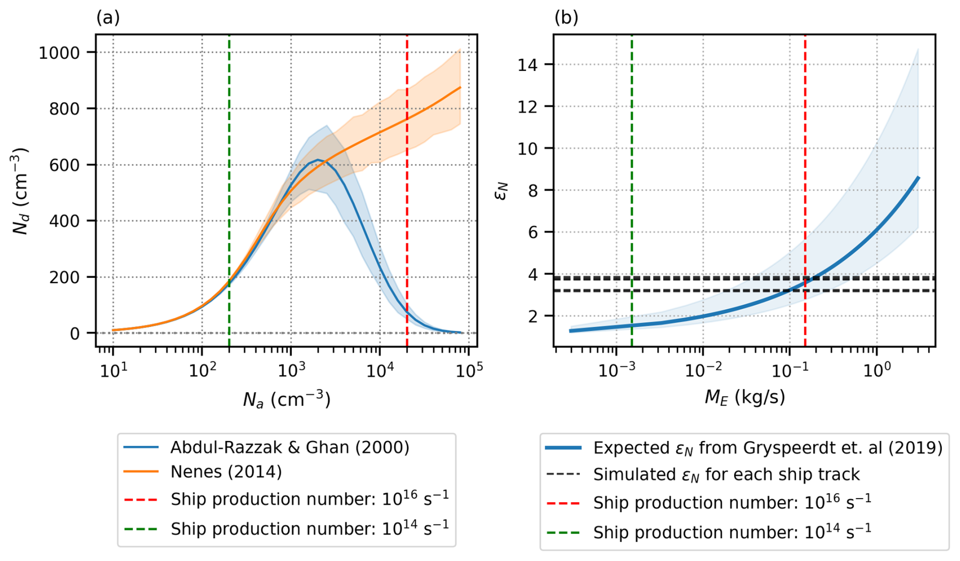
Figure 3 (a) Number of aerosol particles (N_a) activated to cloud droplets (N_d) in different activation parameterisations calculated in a simple adiabatic cloud parcel model. Confidence intervals given by the range of temperature, pressure and updrafts simulated in our case study. (b) The expected enhancement in cloud droplets (ϵ_N) as a function of aerosol mass emission rate (M_E), based on Eq. (1) from Gryspeerdt et al. (2019b). Vertical lines are the emissions from different ship production numbers. Horizontal lines are the enhancements produced from our simulations for each individual ship. Confidence interval is given by the range of background droplet number concentrations in our simulation.

We plot both the ARG and NS (Nenes and Seinfeld, 2003) parameterisations as a function of aerosol number concentration in Fig. 3a, using values of temperature, pressure and updraft velocity that are representative of our domain. We find that with using our realistic ship production numbers (10¹⁶ s⁻¹) the aerosol number concentrations (20 000 cm⁻³) are beyond the critical concentration of ARG, producing the unrealistic split ship tracks. NS, whilst not containing this non-monotonic behaviour, would contain a large over estimation of cloud droplets at the realistic ship production number and therefore would also be unsuitable with these emissions. This detail of the ARG activation parameterisation has been documented in Connolly et al. (2014), and emphasises that commonly used aerosol activation parameterisations are not suitable for MCB applications.

Reduction of our ship production number to 5 × 10¹⁴ s⁻¹, produces only a 200 cm⁻³ aerosol perturbation, but recovers N_d that match much closer to observations. This artificial reduction in ship production number is necessary to obtain more realistic ship tracks (without the splitting effect), but we must verify whether or not the resultant enhancements in these ship tracks is as expected based on observations. Using Eq. (2), we calculate expected enhancements (ϵ_N) based on the background N_d as a function of aerosol mass emission rates. Using our ship production of numbers of 10¹⁶ and 5 × 10¹⁴ s⁻¹, and a mean aerosol mass of $\mathrm{3}\times {\mathrm{10}}^{-\mathrm{18}}$ kg, we obtain mass emissions rates of $\mathrm{1.5}\times {\mathrm{10}}^{-\mathrm{1}}$ and $\mathrm{1.5}\times {\mathrm{10}}^{-\mathrm{3}}$ kg s⁻¹, respectively.

We find that the model enhancement obtained from our reduced emissions are consistent with what we would expect from the real emissions (Fig. 3b), despite the emissions being unrealistically low. Since the enhancements obtained are as expected based on observations, we assume that this reduced ship production number is sufficient to drive this realistic test case, and suitable for evaluation of the model's process representation. For the remaining results of this work, we only simulate ships with ship production number of 5 × 10¹⁴ s⁻¹, however acknowledge that this undermines any ability to make claims relating to the injected aerosol number concentration. As such, we investigate the model representation of the cloud adjustments (specifically LWP adjustments) subsequent to the simulated N_d perturbation, which is of the correct magnitude as established in this section.

3.2 Evaluation of the control

Using the model configuration detailed in Sect. 2.2, our simulation is run for 48 h from 00:00Z 11 July 2018 to 00:00Z 13 July 2018. In our control run, no ship emissions are added to the model, and we use this simulation to characterise our “unpolluted” cloud. Typically, in ship track observations, we have no pure “control” cloud, and therefore we must treat a region outside of a ship track as being representative of what the cloud would have looked like if there was no aerosol perturbation present. In the model case, however, we can simply turn ships on and off to isolate the aerosol impact on the cloud.

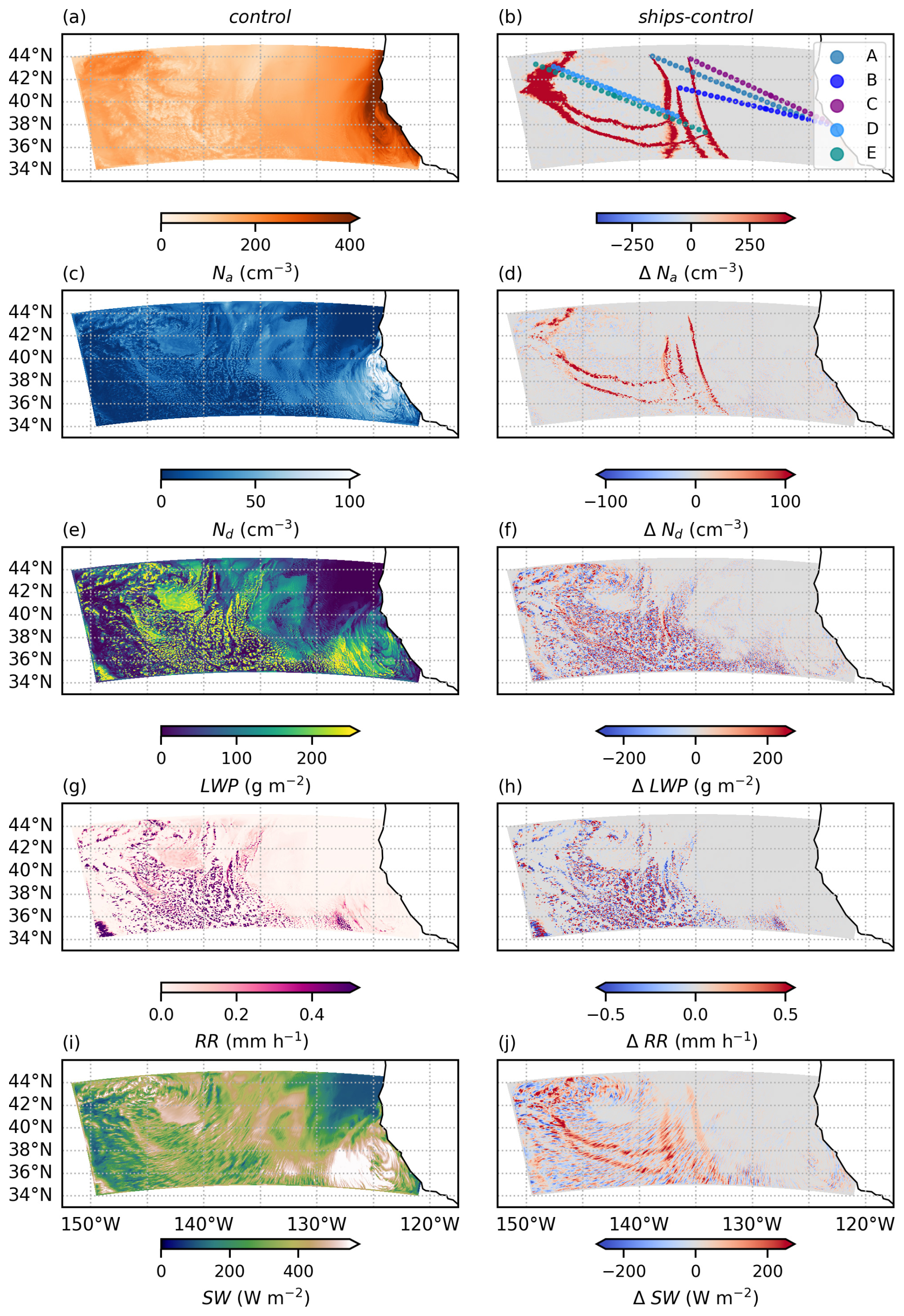
Figure 4 Left column: control simulations of 12 July 2018 at 20:00Z without ship emissions turned on. Panel (b) contains the locations of the ships simulated during this study, up until the time step of this figure. Right column: difference from control for simulation with shipping emissions on. Stochastic noise between two model runs can be seen in the difference plots. Variables shown are aerosol number concentration (N_a), cloud droplet number concentration (N_d), liquid water path (LWP), surface rain rate (RR), and top of atmosphere outgoing short wave radiation (SW). N_d and N_a are mean values across model level numbers below 1 km.

The aerosol number concentration (N_a), cloud droplet number concentration (N_d), liquid water path (LWP), surface rain rate (RR), and top of atmosphere outgoing short wave radiation (SW) for the control run 44 h after initialisation can be found in the left-hand column of Fig. 4. Figure 4a demonstrates how the coupled GLOMAP-mode aerosol scheme allows depletion of aerosol in locations where there is precipitation (in the Central Pacific region of the domain), and the land sources of aerosol are the most significant over the course of the simulation. The coupled UM-CASIM configuration produces open/closed cellular convection in this marine stratocumulus (Fig. 4c in the south-west of the domain), with the presence of drizzle (surface rain rates on average of roughly 0.5 mm h⁻¹; see Fig. 4g).

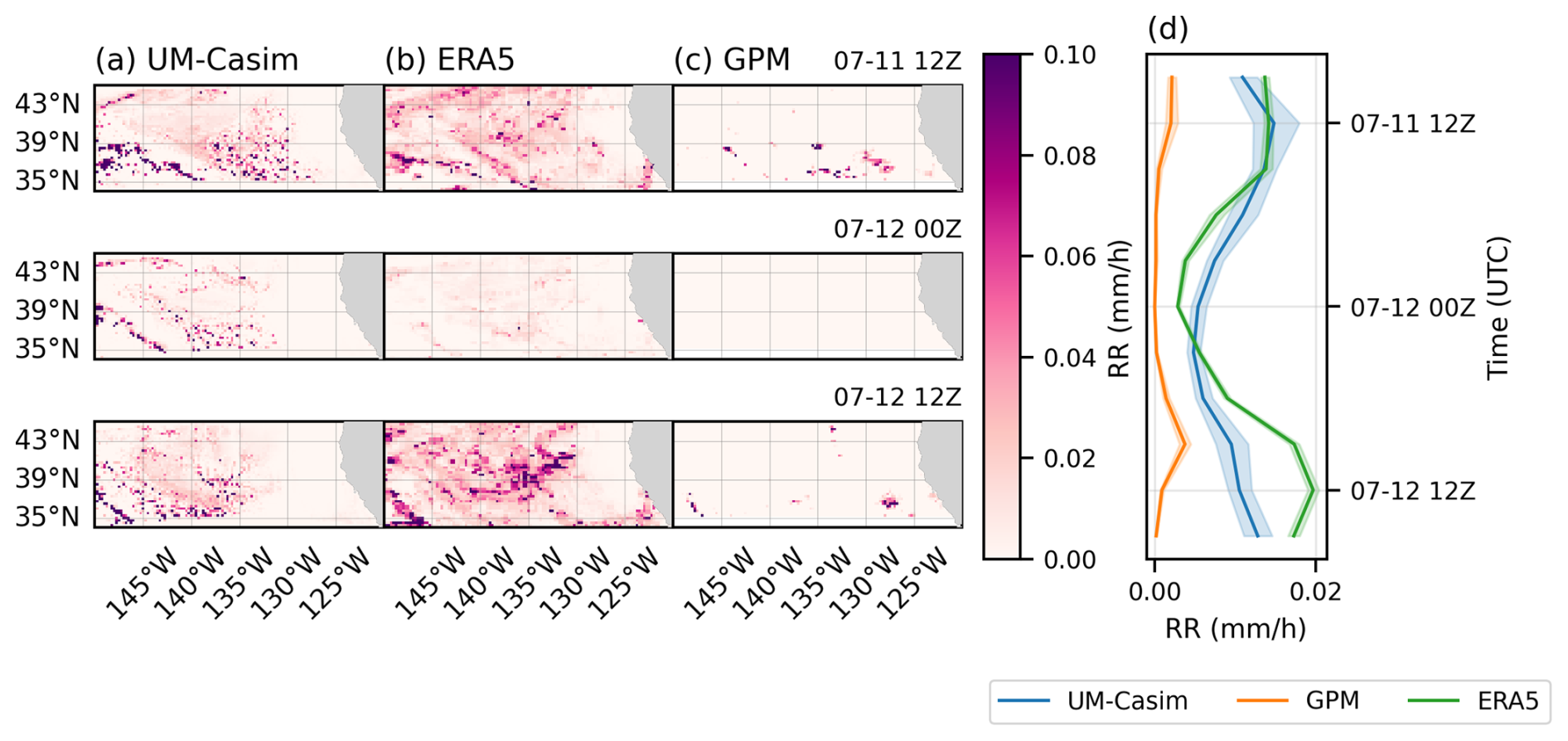
Figure 5 Evaluation of domain wide surface precipitation at 12-hourly intervals. (a) UM-CASIM simulated surface precipitation (regridded to ERA5 resolution), (b) ERA5 surface precipitation, (c) GPM surface precipitation. (d) The domain-wide mean across the simulation runtime, demonstrating the diurnal cycle.

We evaluate our simulated precipitation in Fig. 5. Surface rain rates are shown for UM-CASIM control simulation (regridded to the same 0.25° resolution as ERA5) at 12 hourly intervals, and compared against ERA5 and GPM-IMERG large scale surface rain rates at the same time. Evidently, there is a significant disagreement between ERA5 and GPM on the presence of precipitation in the domain, with GPM being unable to capture drizzle rates smaller than 0.2 mm h⁻¹ (Skofronick-Jackson et al., 2017). UM-CASIM is in rough agreement with ERA5 on the presence, location, and magnitude of the precipitation, however ERA5 contains its own uncertainties in the realism of precipitation (Xiong et al., 2022). The UM-CASIM precipitation rates lie between those from GPM-IMERG and ERA5.

There are 3 overpasses of this domain by the CloudSat Cloud Profiling Radar (CPR; Stephens et al., 2008; Tanelli et al., 2008) during our simulation run. Figure 6a shows the location and presence of surface precipitation (in the 2C-Precip-Column product; Haynes et al., 2009) in these overpasses. There is significant disagreement in between the 2C-Precip-Column and 2C-Rain-Profile (L'Ecuyer and Stephens, 2002) products from the CPR, with UM-CASIM underestimating precipitation along this overpass when compared to 2C-Precip-Column, and having a small mean bias when compared to 2C-Rain-Profile.

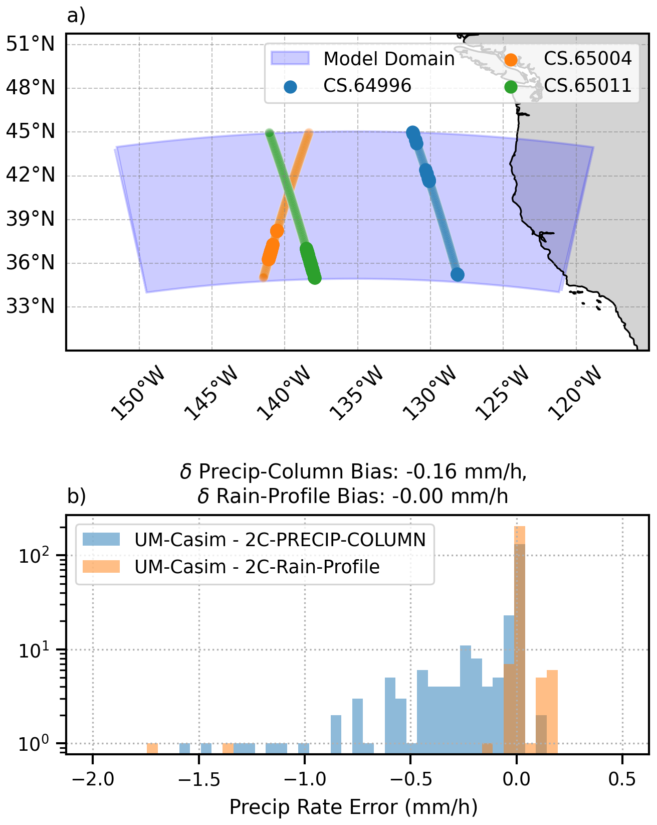
Figure 6 Evaluation of surface against CloudSat CPR products. (a) Location of CloudSat overpasses during the 48 h simulation, with bold points showing locations where surface precipitation from the 2C-Precip-Column product are greater than zero. Associated times of overpass are roughly as follows: CS.64996 at 22:00Z 11 July, CS.65004 at 12:00Z on 12 July, and CS.65011 at 23:00Z on 12 July.

Evidently, this evaluation demonstrates that there is some uncertainty in the simulated precipitation within our domain, as well as within the observed precipitation. The UM-CASIM precipitation falls between what is predicted from ERA5 and GPM, with different CloudSat products giving largely different precipitation rates. More generally, double moment CASIM is shown to have increased skill at representing precipitation in a frontal system over the UK, and a tropical storm in Darwin (Field et al., 2023), as compared to other model microphysics schemes (evaluated against GPM and radar), however there are still limitations in its representation of moderate precipitation, in the range of 4–16 mm h⁻¹ (Bush et al., 2025).

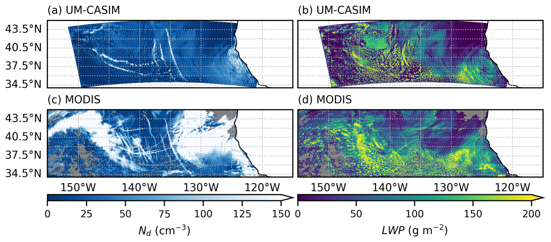
Figure 7 Modelled and Observed N_d and LWP for 12 July 2018 ship tracks. Plotted is a composite of the Aqua and Terra overpasses from Fig. 1, co-located with model nearest output time steps.

With our initialised background aerosol field of 200 cm⁻³, we produce a relatively clean cloud droplet background of roughly 50 cm⁻³. This is largely in line with that seen in satellite observations (Fig. 7a, c), however we note that two large sources of cloud droplets are missing from our model simulation. This is likely due to our initialisation from a constant aerosol field, and therefore we are missing these sources of aerosol in our simulation. Future work in initialising from a more realistic aerosol field would be beneficial, and the limitations of our simplified aerosol configuration are discussed in Sect. 4.1.2. Due to simplifications in the composition of aerosol field, we do not evaluate the model representation of model microphysics and consider mainly the LWP adjustment to the ship N_d perturbation.

3.3 Comparison to observations

As outlined in Sect. 2.1, we evaluate our simulations against three criteria in order to determine the realism of our simulations, and the ability of our model to accurately simulate ship tracks/MCB. In the following sections, we present our findings with respect to each of these criteria.

3.3.1 In-track values

Figure 8 provides a comparison between the mean of all MODIS observations of our ship tracks, and the associated modelled ship tracks (at the nearest time step). The inside track values of both N_d and LWP are a close match between model and observations, with a visible peak in the N_d at early times along track, and a slow increase in LWP with time along track which is consistent with the majority of the tracks moving down a LWP gradient. Due to the missing high N_d region in the Central Pacific part of the domain, ship tracks are only considered up to 15 h along their length, since times longer than this are within this missing high N_d region and therefore accurate comparison between model and observations is not possible due to differences in the background. Obtaining similar N_d values inside the track, and in the background is important for investigations into how the LWP adjusts to the ship induced changes in N_d, and the lifetime of the response, which is discussed further in the following section.

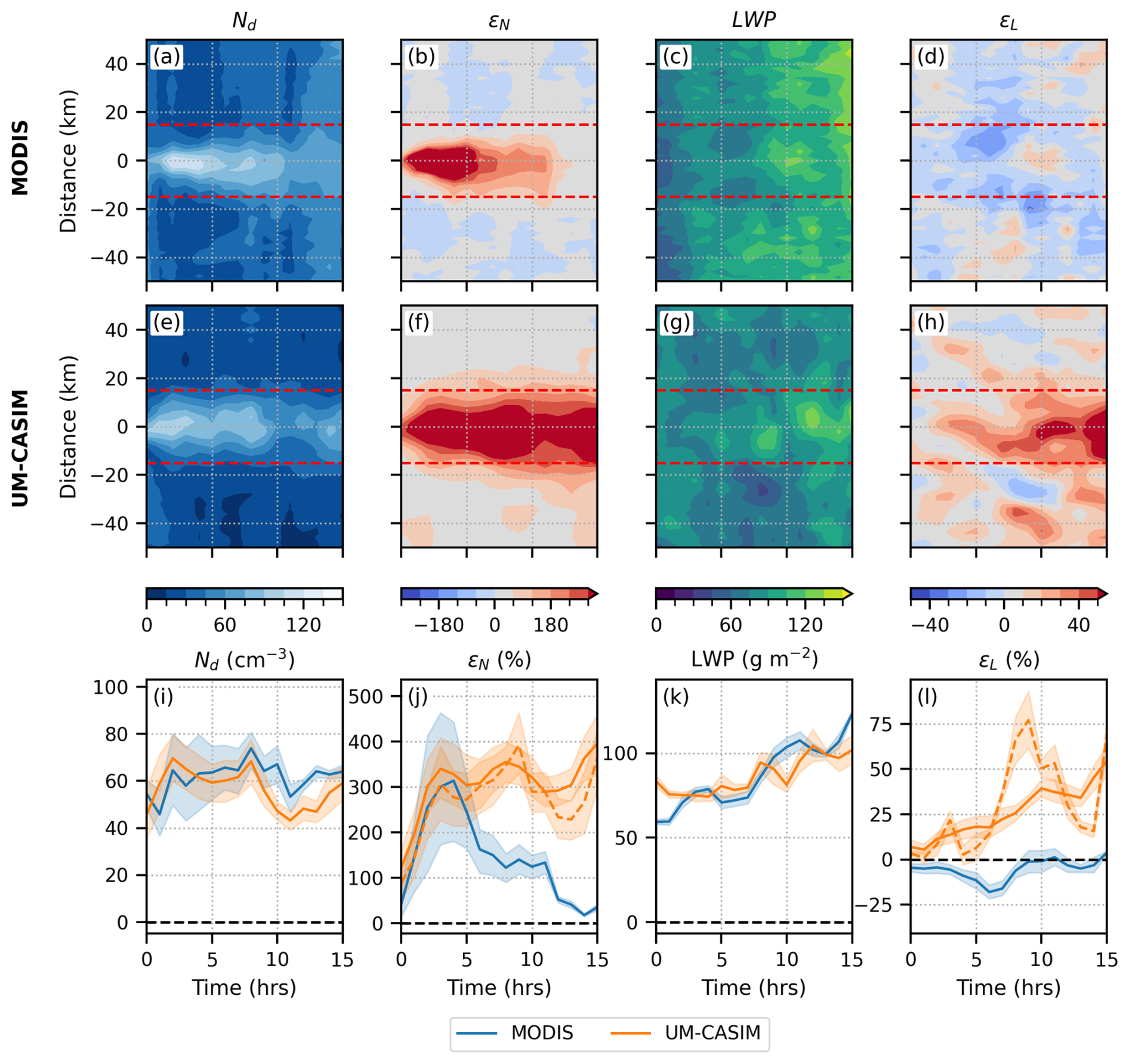
Figure 8 (a–d) Observed N_d and LWP across all observations of our 5 ship tracks, as well as the percentage enhancement of the “inside track” region (defined by < 15 km from the centre). Percentage enhancement is calculated from the mean of the region between 30–45 km away from the centre of the track. (e–h) The same as above, but for modelled ship tracks. The percentage enhancement is instead calculated as the percentage change from the control model run (solid orange line). Percentage enhancement using the lateral offset method (as in the observations) is shown in the orange dashed line. (i–j) Mean of the observed and modelled N_d in-track values, and enhancements, in the “inside track” region. (k–l) The same, but for LWP. Whilst inside-track values for both N_d and LWP are similar between observations and model output, enhancements vary significantly.

The mean percentage errors in the inside track values of N_d and LWP, up to 15 h along the track, are found to be −3.5 % and +3.1 %, respectively. Therefore, for both N_d and LWP the model reproduces observed values to within ±4 %, which is well within our uncertainty from the methods (Sect. 2.6). With respect to our first evaluation criteria, this means that with the artificial reduction in aerosol number concentrations necessary for the activation parameterisation to produce realistic ship tracks (see Sect. 3.1), we are able to successfully reproduce the absolute N_d and LWP values at the location where the aerosol is injected.

3.3.2 Timescales of response

If instead of considering the raw in-track N_d and LWP values, which do not clearly demonstrate the time evolution of the cloud adjustments (since we are not considering a change from an unperturbed state), we calculate the percentage enhancement of the “inside track” region, compared to the “unpolluted” control cloud.

We find that the initial N_d increase and peak of roughly 300 % at 3–4 h is the same in both model and observations. However, despite the in-track values matching very closely between model and observations, the enhancements vary dramatically at longer time scales. In Fig. 8j, the enhancement in N_d is much longer lived than that seen in observations, which instead has returned to the background beyond roughly 15 h. Since tracks are corrected by hand, this observed lifetime is not a result of inaccuracies in ship track location prediction. This highlights the importance of considering the change from the unperturbed state.

Similarly, for the LWP enhancements we see distinctly different responses. In the observations we see the response typically associated with ship tracks in non-precipitating environments, with a decrease in LWP in the first 5 h, which then returns to zero. Conversely, in the modelled ship track we see only a blanket increase in LWP which increases over time. Figure 8k demonstrates that the absolute inside track LWP values are similar, therefore this difference in enhancement must stem from the model representation of the control/background state, and the sensitivity of the model to changes in N_d.

Both the lifetime of the N_d and LWP responses are found to be too long-lived, which suggests that aerosol is not being efficiently removed from the clouds (Wood et al., 2012). This prompts further investigation into which processes are acting unrealistically, and in Sect. 3.3.3 we explore the realism of the simulated ship tracks in two different cloud types: closed MCC and broken cumulus.

Overall, we find that evaluating our model against this criteria in this way reveals issues with the lifetime of the cloud response, and that current set up and formulation of these model parameterisations is unable to capture the observed lifetime of the N_d and LWP changes inside these ship tracks. This will have important implications for the radiative forcing from these ship tracks, since a longer lived response would prolong the brightening inside the ship track, and therefore would cause an overestimated cooling effect.

3.3.3 Sensitivity to initial condition

In Fig. 9, we split our ship tracks into those that occur in different background conditions, as a means to investigate whether our model is able to capture the bi-directional nature of the LWP adjustment that is typically expected. We use direction of travel as a simple proxy for “initial condition” of the cloud before the ship passes, since each grouping of ships is always within approximately 100 km of each other, and therefore experiences largely similar meteorological conditions. Ships A–C follow routes from the coast of California, westwards through the Eastern Pacific (see Fig. 4b). Ships D and E travel towards the coast and are more southerly than ships A–C, through the Central Pacific. The Eastern Pacific ships travel through classic closed mesoscale cellular convective clouds (“closed MCC”), where there are primarily non-precipitating clouds. In the Central Pacific, there are “broken cumulus” that potentially transition into trade cumulus or open MCC, and we see higher occurrence of drizzle at the surface from these clouds (see Fig. S1 in the Supplement). Dividing our enhancements into these two different types of marine boundary layer clouds (Fig. 9), we see that the model is sensitive to the initial condition of the cloud before the ship passes through.

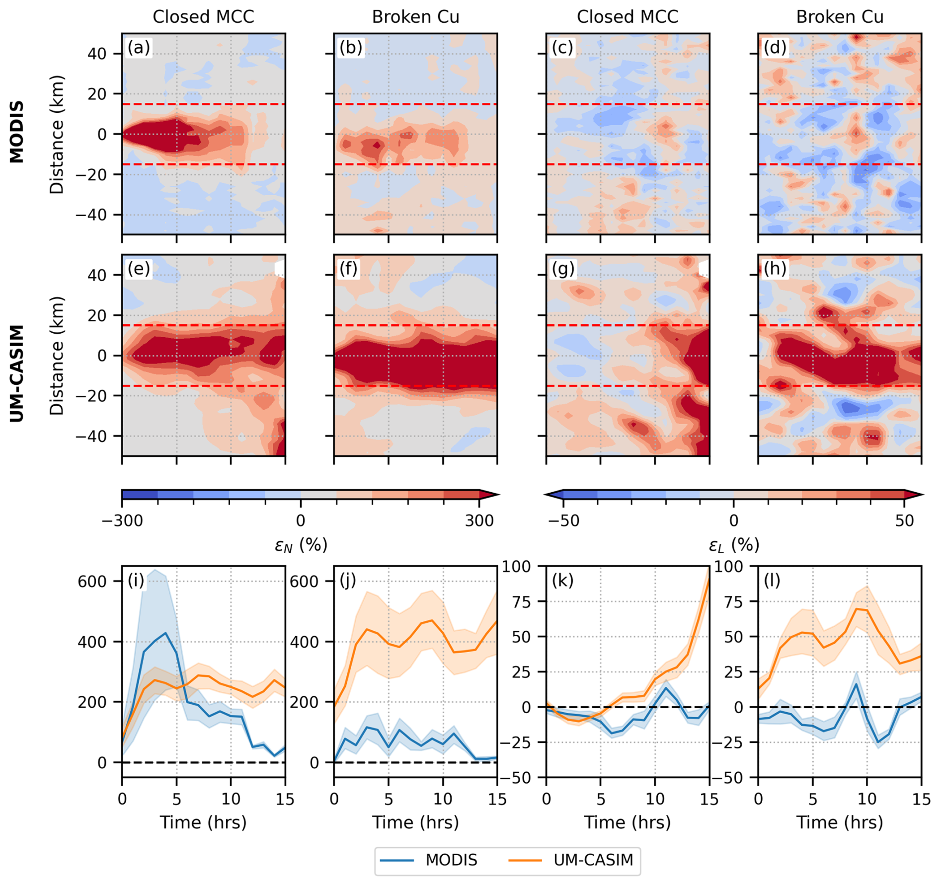
Figure 9 Percentage enhancements from the “unpolluted” references background state. Panels (a)–(d) show observations of ship tracks in in the Eastern Pacific region of the domain (ships A–C) and the Central Pacific region (ships D & E) conditions for N_d (left) and LWP (right). Panels (e)–(h) show the same but for modelled ship tracks. Panels (i)–(l) show the average of the “inside track” region, as defined by the red dashed lines in panels (a)–(h).

In closed MCC (Fig. 9, 1st and 3rd column for N_d and LWP enhancements, respectively) we find similar enhancements in the model and observations. Shortly after the ship passes there is better agreement, with observations and model simulations matching within the uncertainty in the first 5 h. Following this, we see divergence between the two. This could be in part due to our tuning of the aerosol emissions to satisfy the non-monotonic behaviour of the activation parameterisation and reproduce correct N_d enhancements on short time scales. We would still expect the response from weaker aerosol perturbations to reduce over time, and therefore there must be some process within the model allowing for this increased N_d perturbation lifetime. A potential source of this long-lived N_d enhancement could be inefficient removal of cloud droplets by entrainment. In these clouds, we see larger simulated LWP enhancements from 10–15 h after the ship passes, therefore weak entrainment rates could correspond to the large N_d enhancements at these times also. Additionally, even in these closed MCC conditions where we do not observe much drizzle (Fig. S1), if cloud droplets cannot become rain droplets via accretion or autoconversion, or if larger droplets cannot sediment out, then the removal of aerosol will be underestimated and reinforce the N_d perturbation. A thorough analysis of the output process rates is needed to fully identify the source of this long-lived N_d perturbation.

Considering the ships that travel through broken cumulus clouds (Fig. 9, 2nd and 4th column for N_d and LWP enhancements respectively), we see significant disagreement between the observations and the model. This suggests that the large disagreement in Fig. 8 is largely due to the ship tracks in these conditions where precipitation is more prevalent. The N_d enhancement is too large, and shows no sign of diminishing even after 15 h after the aerosol perturbation. This suggests that the model is not only overly sensitive to aerosol in broken cumulus clouds, but is not effective enough at removing aerosol from the cloud either. Additionally, the LWP adjustment is a different sign between model and observations. This suggests that the model is far too keen to suppress precipitation in these conditions, leading to large increases in LWP that are not observed in the satellite imagery.

There is some uncertainty that may be introduced due to the missing cloud structure in the Central Pacific region in our simulation, causing our background state to look cleaner than it should be. This missing cloud structure, however, will only influence the ship track over 10 h along the track, and therefore is not the source of the large overestimation in N_d enhancement seen before 10 h along the track in Fig. 9j.

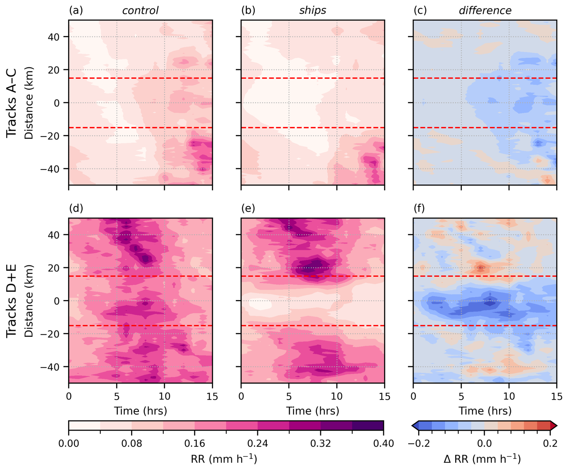
Figure 10 Surface rain rate, averaged across two groupings of tracks (ships A–C and D + E), across 24 h on 12 July 2018, for the ships and control runs, as well as the difference between the two. The figure shows clear precipitation suppression in the broken cumulus case, with rain rates reduced to almost zero. Some precipitation suppression in the closed MCC case (ships A–C) since there is actually some precipitation towards the end of the model run (see Fig. S1).

In Fig. 10, we show the surface rain rates inside our ship tracks, compared to the control run. Here, we see that for tracks D and E in the broken cumulus region (where there are larger precipitation rates), the precipitation is essentially completely shut off which is likely a far too strong response, since precipitation in high N_d conditions does occur (Gryspeerdt et al., 2022).

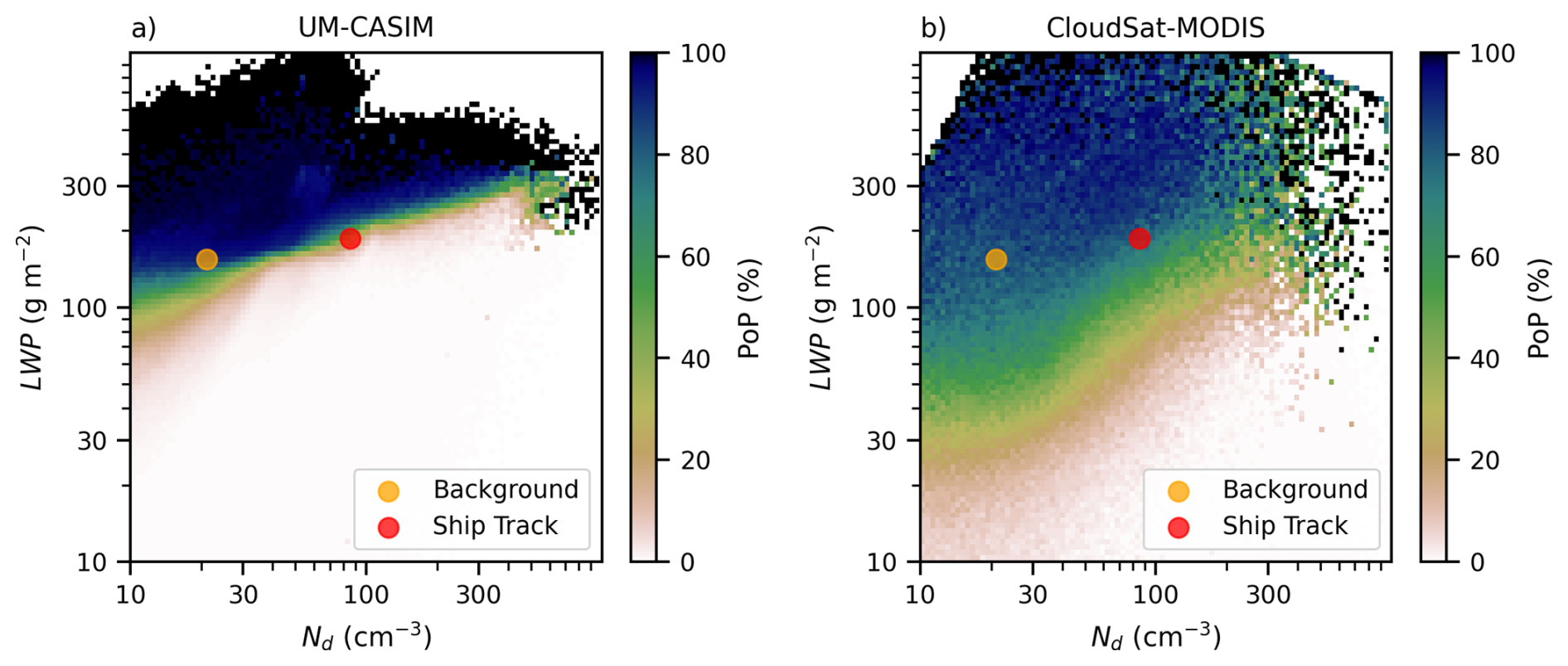
Figure 11 The probability of precipitation (PoP) in N_d-LWP space, in UM-CASIM simulations compared to CloudSat-MODIS collocated observations for the same domain. UM-CASIM has much faster transition from precipitating to non-precipitating with changes in N_d than observed. The orange point is the background (control) N_d and LWP for our precipitating ship (D–E), and the red point is the N_d and LWP inside the ship tracks, averaged over the simulation run time.

We demonstrate this in Fig. 11, where the probability of precipitation (PoP) is plotted in N_d-LWP space for (a) our 48 h model simulation and (b) 4 years of collocated CloudSat-MODIS observations (following a similar methodology to Gryspeerdt et al., 2022). The distribution of PoP within this N_d-LWP space is a representation of microphysical processes, and shouldn't differ significantly seasonally or day-to-day, therefore a comparison between a two-day simulation and four years of observational data should represent the same distribution (see Fig. S2).

The very sharp gradient in PoP with increases in N_d demonstrates the high-sensitivity of the autoconversion scheme to aerosol. In our broken cumulus case, the addition of ship aerosol moves our “background” point in N_d-LWP phase space just over the sharp boundary in PoP to our “ship track” point. This explains the complete precipitation suppression in these cases, since this gradient is so sharp. In observations, there would be a small decrease in PoP, but not to the same extent.

In our simulations, we do see that there is some sensitivity to the initial conditions since we obtain different responses in different cloud structures (closed MCC vs. broken cumulus). We can conclude that the model is more at representing LWP adjustments in closed MCC conditions where there is little precipitation, at least for up to 5 h. However, in the case of broken cumulus clouds with higher occurrence of precipitation, current model parameterisation formulations are not suitable to accurately simulate these scenarios, and the lifetime of the response is far too long lived.

4 Discussion

In this study, we produce convection permitting simulations of ship tracks using a regional model and double moment microphysics scheme, exhibiting its capabilities and limitations in simulating N_d perturbations and LWP adjustments within clouds. We evaluate our case study against three criteria, which are designed to ensure ship track simulations contain an accurate representation of cloud processes, and therefore may be a useful tool for MCB research.

Adjusting ship emissions to 5 × 10¹⁴ particles per second as to avoid unphysical behaviour in the activation parameterisation, we reproduce realistic absolute values of N_d and LWP inside simulated ship tracks, and find that in closed MCC (non-precipitating conditions) the enhancement in N_d and LWP from the control “unpolluted” cloud is well modelled for the first 5 h. However, beyond this, the lifetime of the response is too long lived. This is driven by the representation of parameterisations at very high aerosol number concentrations.

4.1 Limitations

4.1.1 Definition of “precipitating” and “non-precipitating” clouds

In this work, we divide our ship tracks into those that occur in “closed MCC” clouds (tracks A–C), and those in “broken cumulus” (tracks D & E). When evaluating against satellite observations, we find that our model performs better in these closed MCC cases, and worse in the broken cumulus. We attribute the difference in behaviour of the model in these different cloud types as being due to the representation of precipitation by the model. The closed MCC clouds in our model have higher background CCN concentrations (Fig. 4a) and greater N_d (Fig. 4b) with less precipitation (Fig. 4g), whereas the broken cumulus have heavier precipitation (Fig. 4g). This is in line with what is expected in these cloud types in literature (Alinejadtabrizi et al., 2024). We find that precipitation is too easily suppressed and therefore ship track lifetimes are too great in clouds where there is precipitation (such as our broken cumulus). Non-precipitating clouds (such as our closed MCC) are less impacted by these, and therefore the model produces more realistic simulations of these clouds.

However, there are many differences between closed MCC and broken cumulus other than amounts of precipitation that may impact this analysis. In Fig. 4 “control” column the difference between the Eastern Pacific closed MCC and Central Pacific broken cumulus can be observed. Closed MCC have greater cloud fraction (CF), as seen in Fig. 4c, which impacts the spatial scale over which aerosol can impact the clouds. The simulated marine boundary layer (MBL) height increases with distance from the coast and is roughly 550 m in the Eastern Pacific, deepening to 900 m in the Central Pacific (not shown). In the deeper MBL, is is possible that aerosols may not reach cloud base as readily (Bretherton and Wyant, 1997), which could be a potential reason why satellite observations of tracks D & E do not show significant LWP enhancement – the model may be mixing aerosol vertically too efficiently in these clouds, therefore the perturbation to N_d is too great. Alternatively, broken cumulus regions can exhibit higher latent/sensible heat fluxes and weaker subsidence (Wood and Bretherton, 2004), creating a deeper MBL with weaker entrainment rates. If entrainment is too weak, however, then LWP anomalies inside the ship tracks will be allowed to exist for too long (Fig. 8j and l).

Additionally, within this single case study, we are restricted in the extent to which we can divide our tracks into “different conditions”. All these tracks still occur within the same domain on the same day, therefore there is a limitation on how different the conditions can be, especially since all ships converge on the same region in the centre of the domain. A more comprehensive statistical analysis is necessary to determine fully the behaviour of the model across many cloud types and conditions, which is not possible with a single 48 h case study.

4.1.2 Aerosol scheme

In this work, our simulations are initialised from a simplified aerosol field of solely accumulation mode aerosol. This produces realistic accumulation mode aerosol, but underestimates aerosol mass/number concentrations in the Aitken or coarse modes (since these will only be contributed to by the background emissions detailed in Sect. 2.2). An evaluation of the sulphate mass mixing ratio and the simulated AOD against CAMS reanalysis are provided in the Supplement (Fig. S3), and are found to only have small spatial differences. However, neglecting other aerosol components (which are significant; Fig. S4) might impact the formation of cloud droplets and the initiation of precipitation in this work (although we find that the precipitation representation is reasonable; Fig. 5). Whilst initialising from a single aerosol mode appears to reproduce the AOD from CAMS, this does not ensure accurate representation of the size distribution which could, in turn, influence the simulated response to additional aerosol.

These other aerosol components, such as organic matter and sea salt, which are likely to be present in this case (Fig. S4), will have both different hydroscopicities and different sizes, which can affect cloud droplet formation and the initiation of precipitation. For example, sea salt can modulate the activation of sulphate nuclei into cloud droplets (Fossum et al., 2020), therefore inclusion of even small concentrations of sea salt aerosol may reduce N_d concentrations. McCoy et al. (2018) also found that increasing sea salt concentrations limits N_d due to reduction in supersaturation by the larger sea salt CCN. This effect occurs because of the different hydroscopicity of sea salt, but also its larger size, making it an effective CCN. This neglecting of other aerosol components with different hydroscopicities should not significantly impact cloud droplet number concentrations or initiation of precipitation, however the neglecting of aerosols with different sizes may impact our analysis, since the size of the aerosol mode remains the more important factor for cloud nucleating ability of aerosol particles (Dusek et al., 2006). The initialisation from solely accumulation-mode aerosol may also lead to an inaccurate representation of aerosol surface area, which in turn can affect vapour sinks through condensation as well as rates of new particle formation. In addition, the absence of an Aitken mode removes a pathway for particle growth and may result in an underestimation of cloud condensation nuclei (CCN) concentrations. Since the simulations span only 48 h, there is insufficient time for the aerosol population to evolve toward a more realistic size distribution, despite background emissions into other modes.

Grosvenor et al. (2017) use a similar initialisation from a uniform field of accumulation mode in CASIM, and find that the resultant N_d is approximately as seen in observations. Similarly, in our simulations we find that our background cloud droplet number concentrations are within 15 cm⁻³ between UM-CASIM and MODIS observations, with our model only slightly underestimating background droplet number concentrations. For the purposes of this study, the main requirement of our simplified aerosol configuration is to produce a realistic background cloud droplet field which can then be perturbed by extreme ship aerosol emissions, so the model representation of the subsequent adjustments can be investigated. Crucially, the aims of this work are to investigate LWP adjustments to N_d perturbations inside ship tracks, which are applied in a more realistic method to previous work by using aerosol perturbations at real ship locations. As such, no conclusions about the model representation of the aerosol microphysics can be made. The emissions from the ships are not what the actual ships emitted, and are constant across all 5 ships. Furthermore, the emissions are then tuned to reproduce realistic N_d values inside the ship track, since the activation scheme is found to be unsuitable. Then, the subsequent adjustments in LWP (which are dependent on the absolute N_d value) are investigated. Whilst there may be some slight inaccuracy in our initial background N_d field from neglecting other aerosol components with other size modes, this is unlikely to be the cause of the large discrepancies in the lifetime of the LWP response in the ship tracks between observations and model. Future work with a more comprehensive aerosol configuration would be beneficial in order to reduce any uncertainty in the interactions between different aerosol size modes and their impacts on cloud droplet activation in ship tracks.

Additionally, our coupling between CASIM and GLOMAP-mode aerosols (as described in Gordon et al., 2020) means that the removal of aerosol from the cloud is only possible through wet-scavenging. Autoconversion and accretion rates determine the rate of removal of aerosol by precipitation, however cloud microphysical processing of the aerosol is not implemented, meaning that there is no reduction of N_a by collision-coalescence of cloud droplets, nor an increase in N_a through droplet evaporation (Gordon et al., 2020). This severely limits the mechanisms by which aerosol can be removed from the cloud, since collision-coalescence scavenging is an important sink of CCN (Kang et al., 2022; Terai et al., 2014) and may explain our long-lived N_d enhancements within our ship tracks. Once precipitation is even slightly suppressed, aerosol removal from the cloud is also significantly reduced, N_d remains high (Wood et al., 2012), and therefore ship track lifetimes are too long. In Fig. 11 we see that very small increases in N_d are able to cause an almost complete suppression of precipitation (as a result of our autoconversion parameterisation), which in turn will feedback on the lifetime of the N_d response, since aerosol will continue to exist in the cloud. This indicates that cloud processing is important for accurately simulating ship tracks, as to avoid this precipitation suppression feedback.

4.1.3 Definition of the “control” region

When there are fewer background sources of aerosols, it is easier to define the “unperturbed” cloud using the region adjacent to the ship track. When there are more ships, or other sources of aerosols, this definition becomes more difficult and becomes a greater source of uncertainty. Other studies have explored alternative methodologies of gaining insight into the unperturbed cloud in observations (such as through the use of ML algorithms; Diamond et al., 2020; Chen et al., 2022; Diamond, 2023), however will still struggle with increasingly complex and polluted backgrounds.

This has important implications for the design of field experiments of MCB. In order to isolate the aerosol effect with greatest certainty, a relatively homogeneous background is necessary. If there are many overlapping ship tracks/interacting sources, this definition of the control becomes more nuanced, and additional uncertainty is introduced. If field trials were to occur for MCB, the easiest, and best attribution of the aerosol effect could be made if ships tracks were not allowed to interact, and the background was not too heavily polluted with sources that were difficult to define.

4.2 Suitability of parameterisations for high-concentration aerosol perturbations

We confirm that the commonly used activation parameterisation by Abdul-Razzak and Ghan (2000) is inadequate to simulate aerosol-cloud interactions at very high aerosol number concentrations. We demonstrate the potential result of the non-monotonicity of the ARG activation when simulating ship tracks – ship tracks appear split (Fig. 2). In practical terms, this necessitates an artificial reduction in ship aerosol emissions to obtain ship track structures that resemble those seen in satellite imagery. While this workaround may yield visually plausible results in non-precipitating conditions, it undermines the physical realism of the simulation's temporal evolution. An alternative activation parameterisation from Nenes and Seinfeld (2003) would also be unsuitable at these high aerosol number concentrations, as activated cloud droplet concentration would be overestimated. Further work is necessary in determining whether other parameterisations (such as that of Shipway and Abel, 2010) would be suitable, or if entirely new schemes for high aerosol number concentrations are needed.

We find that model-observation discrepancies become more pronounced in broken cumulus clouds, where there is greater precipitation. Under such conditions, it is possible that the autoconversion parameterisation of Khairoutdinov and Kogan (2000, KK00), which governs the conversion of cloud water to rain, is too sensitive to increases in N_d. This scheme tends to suppress production of rain droplets too readily when the cloud droplet number concentration (N_d) is high – as demonstrated by the complete shut off of precipitation inside these ship tracks that form in precipitating scenes (see Fig. 10).

In Fig. 11, the PoP is almost binary in our simulation, with either 100 % chance of precipitation above some threshold N_d-LWP line, and almost 0 % chance below it. In observations, there exists a much wider space in which precipitation can occur. This means that for any conditions close to this threshold line in N_d-LWP in our simulation, a small increase of N_d (such as through the injection of ship emissions), will move us beyond this threshold and decreases the PoP too extremely.

Consequently, the model predicts unrealistic suppression of precipitation, resulting in overestimation of the ship track lifetime and, by extension, the radiative cooling associated with the perturbation. This is not surprising, since the KK00 autoconversion scheme was designed for mid-latitude and extratropical stratocumulus layers under typical meteorological conditions, with their evaluated “polluted” case only having an N_d of 175 cm⁻³. This is aligned with the findings of Jing and Suzuki (2018) with respect to GCM parameterisations, where precipitation inhibition can lead to a wet scavenging feedback which can increase aerosol loading somewhat non-physically. KK00 is possibly not well-suited to simulate very high N_d perturbations, as it tends to easily suppress precipitation – even in conditions where precipitation could still occur.

As discussed in Sect. 3.2, there is some uncertainty in the realism of the simulated precipitation in the domain, since it is difficult to obtain conclusive precipitation measurements across different satellite and reanalysis products. In order for the enhancement of LWP in a ship track to occur, precipitation need only be suppressed at cloud base, and therefore it is also possible that no impact in surface precipitation would occur. This highlights the difficulty in evaluating not only precipitation in models, but specifically the precipitation suppression effect.

In their designed configurations, these parameterisations limit the ability of models to provide meaningful insight into high N_d perturbations and subsequent adjustments over longer timescales or under precipitating conditions. This has important implications with respect to modelling across many scales, not just regional simulations. The development of global cloud resolving models would also benefit from improved cloud microphysics parameterisations (Satoh et al., 2019).

Additionally, for simulations aimed at informing MCB strategies, it is particularly critical that parameterisations are suitable for high-N_d scenarios. Without modifications, models will likely overstate the cooling impacts, leading to inaccurate assessments of MCB efficacy. Improved autoconversion schemes that remain valid at high N_d (such as a scheme where autoconversion rate does not tend to zero as quickly with increases in N_d for a given LWP, allowing for a more diffuse PoP within N_d-LWP space), along with more robust activation parameterisations that avoid the need for artificial aerosol reductions, and the inclusion of cloud-processing such that precipitation suppression feedbacks are avoided, are essential for advancing the realism of such simulations.

5 Conclusions

Accurate model representation of aerosol-cloud processes is essential for reducing uncertainty in climate projections and simulating the impacts of marine cloud brightening (MCB). Ship tracks provide a “natural experiment” for isolating the aerosol effects on clouds, and gaining information about the time evolution of the cloud response. In order to evaluate the simulated LWP adjustments to a N_d perturbation, we simulate a real case of ship tracks observed off the coast of California on 12 July 2018, using an experimental configuration of the Met Office's UK weather forecasting model.

We evaluate the performance of our model against three criteria, aiming to produce simulations of ship tracks which are a useful tool for investigating the impacts of MCB. We assess the model's ability to reproduce observed relative and absolute changes in cloud droplet number concentration (N_d) and liquid water path (LWP), using MODIS satellite retrievals for validation. The ship tracks occur within a marine stratocumulus deck under moderately clean background conditions, including pockets of drizzling cloud.

We find that the activation parameterisation of Abdul-Razzak and Ghan (2000, ARG) is not well-suited for simulating high aerosol number concentrations typical of ship plumes. In particular, ARG exhibits non-monotonic behaviour at elevated concentrations, leading to non-physical results unless aerosol input is artificially reduced by a factor of 20 (Fig. 3). This adjustment yields raw N_d and LWP values within ship tracks that closely match observations (Fig. 8). An alternative activation parameterisation, from Nenes and Seinfeld (2003, NS), is found to overestimate expected N_d at high aerosol number concentrations when evaluated in a simple adiabatic parcel model (Fig. 3). Further work is necessary to fully evaluate other activation parameterisations (such as that of Shipway and Abel, 2010) at these high concentrations and determine whether modifications can be made to existing schemes, or if novel ones must be developed.

Analysis of raw values inside ship tracks does not tell us about the time evolution of the LWP adjustments, or how long it takes the clouds to return to the unperturbed state. In the model, this is easy to define through the use of a control simulation. In the observations, we consider the region just outside of the ship track as a representative control region. This highlights the usefulness of ship tracks in observing aerosol-cloud interactions, as it provides us with this control region that is otherwise so hard to define. When considering the enhancements from the control state, we find that the model fails to accurately simulate the time evolution of the response that is seen in observations (Fig. 8). Specifically, model enhancements in N_d persist too long, and the LWP response diverges in sign from observations. On average, across five simulated ship tracks, the model does not capture the correct time evolution of the N_d response or LWP adjustments. There is some uncertainty (roughly 10 %) introduced by the definition of the control state in the observations, since it is difficult to define the unperturbed cloud when there are many overlapping ship tracks. Additionally, some of this discrepancy could be attributed to a distortion in the time evolution due to the reduction of ship emissions (to better match the observed tracks, and avoid “split” tracks).

We further classify ship tracks by background precipitation conditions to better understand this discrepancy (Fig. 9). In non-precipitating closed MCC clouds, the model captures the initial enhancement in cloud properties but still exhibits a response that is too long lived compared to observations (Fig. 9i, k). This suggests that while the initial tuning of the activation parameterisation produces realistic tracks, it may distort the subsequent cloud evolution, and points to the broader need for improved activation schemes capable of handling extreme aerosol conditions, especially in contexts such as MCB (Connolly et al., 2014).

In precipitating environments, model-observation disagreement is more pronounced, which is critical for studies of cloud adjustments to aerosols. Model N_d enhancements are significantly overestimated and show no decay over time, whereas observations indicate a return to background values within 15 h (Fig. 9j). Moreover, the model shows a strong positive LWP adjustments, while observations show a weakly negative one. This suggests that the model either (a) overestimates the sensitivity of precipitation suppression to aerosol, (b) misrepresents background precipitating conditions (Fig. 11), or (c) does not sufficiently remove aerosol from cloud.

Any model overestimation of the LWP adjustment has particular relevance for solar radiation management proposals such as MCB, and forcing estimates of cloud adjustments in km-scale models. Simulating N_d perturbations accurately on the individual cloud level is an exceptionally difficult task for the field, and robust evaluation of model representation at these scales is necessary. Current model parameterisations may cause an overestimation in the cloud responses to aerosol and predict an unrealistically strong cooling effect, especially under precipitating conditions. Any application of these models to unobserved phenomena like MCB must be grounded in rigorous comparison with real-world observations, and further work is necessary in modifying parameterisations such that they are more suitable for high-concentration N_d perturbations.