Technical note: Comparing ozone production efficiency (OPE) of chemical mechanisms using chemical process analysis (CPA)

Chemical mechanisms are critical to chemical transport models for air quality research and policy analysis. Several mechanisms are available and intercomparison, especially using metrics which reduce sensitivity to modeling scenario, is important for interpreting results and assessing uncertainties. Here, we investigate Ozone Production Efficiency (OPE) as a comparison metric under conditions where nitrogen oxides (NO_X) are limited. OPE is the net number of ozone molecules produced per NO_X molecule lost and can be computed in simulations using chemical process analysis (CPA). We compute OPE (OPE-CPA) for four chemical mechanisms (CB6r5, CB7r1, SAPRC07, RACM2) and find a similar response to varying anthropogenic emissions of volatile organic compounds (VOC) and NO_X. RACM2 consistently produces the largest OPE-CPA and differences between mechanisms are greatest at high VOC $/$ NO_X ratios. The high RACM2 OPE-CPA is partially due to a slower OH+NO₂ rate and potentially to its treatment of NO_X recycling. OPE-CPA is generally consistent with aircraft OPE measurements downwind of Houston but direct comparison is difficult due to uncertainties in deposition and VOC speciation. More recent OPE measurements are required to determine whether trends over time are consistent. OPE-CPA responds nonlinearly to NO_X and increases at low NO_X even as ozone production decreases. Using OPE to predict ozone response to NO_X emissions reductions is therefore an oversimplification that will tend to overstate ozone reductions. OPE-CPA is a viable metric to compare mechanisms, however, additional work would be helpful to define standardized conditions for comparisons.

1 Introduction

Three-dimensional Chemical Transport Models (CTMs) provide a representation of the atmospheric processes leading to the formation of secondary pollutants such as ozone (O₃) and particulate matter<2.5 µm (PM_2.5). Regulatory agencies use CTMs as one of their tools to determine what anthropogenic emissions to control and by how much to achieve the U.S. National Ambient Air Quality Standards (NAAQS) for O₃ and PM_2.5. Key components of CTMs are the gas-phase chemical mechanisms that connect primary emissions to secondary pollutants. CTMs require efficient, condensed chemical mechanisms and multiple mechanisms are currently available for preparing US emission control strategies, including the Carbon Bond version 6 revision 3 (CB6r3) (Emery et al., 2015); the Statewide Air Pollution Research Center 2007 (SAPRC07) (Carter, 2010a); and the Regional Atmospheric Chemistry Mechanism version 2 (RACM2) (Goliff et al., 2013). These mechanisms have been included in both the U.S. Environmental Protection Agency (EPA) Community Multiscale Air Quality Model (CMAQ) and the Comprehensive Air Quality Model with Extensions (CAMx). Current versions of CAMx include more recent versions of the Carbon Bond mechanism, CB6r5 (Yarwood et al., 2020) and CB7r1 (Yarwood et al., 2021).

Mechanism intercomparison is important to interpreting results and assessing uncertainties. Several recent studies compare O₃ formation when selected mechanisms are used in the same model with equivalent emissions for all mechanisms (Bates et al., 2021; Chen et al., 2024; Derwent, 2017, 2020; Place et al., 2023; Shareef et al., 2022). Standardized metrics, such as the Maximum Incremental Reactivity (MIR) factor (Carter, 1994), are useful for mechanism comparisons since they reduce sensitivity to the modeling scenario. MIR is useful for comparing O₃ forming tendency of volatile organic compounds (VOCs), $d{\mathrm{O}}_{\mathrm{3}}/d\mathrm{VOC}$, under VOC-limited conditions. In recent years, O₃ formation in the US has become limited on days exceeding the NAAQS by the availability of nitrogen oxides (${\mathrm{NO}}_{\mathit{\text{X}}}=\mathrm{NO}+{\mathrm{NO}}_{\mathrm{2}}$) or trended toward this limitation, except in major urban centers (Blanchard and Hidy, 2018; Tao et al., 2022; Chen et al., 2023; Acdan et al., 2023). There is therefore a need for a comparison metric suitable for NO_X-limited conditions.

A key descriptor of NO_X-limited O₃ formation is the net Ozone Production Efficiency (OPE), which is the net number of O₃ molecules produced per NO_X molecule lost (Kleinman et al., 2002). Here, net O₃ produced is the difference between O₃ produced by chemical reactions minus O₃ lost by reactions. In this study, we investigate OPE as a metric for comparing mechanisms under NO_X-limited conditions using a 2-box configuration of CAMx. Prior work using the Decoupled Direct Method (DDM) to calculate OPE (OPE-DDM) in 3D simulations encountered difficulties accounting for effects of deposition (Henneman et al., 2017). We investigated using OPE-DDM in this study but encountered non-intuitive results such as computing zero OPE-DDM when O₃ was clearly increasing. Instead, we use chemical process analysis (CPA) to compute OPE and compare results among four chemical mechanisms – CB6r5, CB7r1, SAPRC07, and RACM2. Simulations were performed for three Texas cities during typical high ozone events during the 2019 ozone season. We also reviewed available measurements of OPE and conducted simulations to represent measurements years to compare measured and modeled OPE.

2 Methods

2.1 OPE measurement review

We reviewed the published literature from year 2000 forward to find OPE estimates from ambient measurements in the eastern US for comparison to our modeled OPE results. We found OPE estimates from aircraft and surface measurements in various locations, the earliest measurements being in 2000 and the latest in 2023. We did not re-analyze any of the measurements but used the OPE estimates obtained by the data collection teams.

Because our modeling is conducted for Texas cities, we focused on the aircraft measurements in transects of the Houston plume during the Texas Air Quality Study (TexAQS) 2000 (Ryerson et al., 2003; Daum et al., 2003, 2004; Zhou et al., 2014), TexAQS 2006 (Zhou et al., 2014; Neuman et al., 2009), and Deriving Information on Surface Conditions from Column and Vertically Resolved Observations Relevant to Air Quality (DISCOVER-AQ) in 2013 (Mazzuca et al., 2016). For a regional area in the southeast US (not including Texas), Travis et al. (2016) estimated OPE from aircraft measurements during the Intercontinental Chemical Transport Experiment – North America (INTEX-NA) in 2004 and the Studies of Emissions and Atmospheric Composition, Clouds and Climate Coupling by Regional Surveys (SEAC4RS) campaign of 2013. Hembeck et al. (2019) give OPE estimates for the Baltimore area from aircraft flights during DISCOVER-AQ in 2011. Chace et al. (2025) estimated OPE from aircraft measurements in the urban plumes of New York City, Chicago, and Los Angeles in 2023 during the Atmospheric Emissions and Reactions Observed from Megacities to Marine Areas (AEROMMA) campaign. Data from surface sites over extended periods of one or more months have also been used to estimate OPE (Griffin et al., 2004; Blanchard and Hidy, 2018; Ninneman et al., 2017, 2019).

Net OPE can be estimated from atmospheric measurements by multiple methods. The most common method is to plot the O₃ or odd oxygen (O_X) concentration as a function of the NO_Z concentration from collocated measurements. NO_Z is usually determined as ${\mathrm{NO}}_{\mathit{\text{Z}}}={\mathrm{NO}}_{\mathit{\text{Y}}}-{\mathrm{NO}}_{\mathit{\text{X}}}$ with NO_Y being the total reactive odd nitrogen. However, NO_Z is sometimes determined by summing measurements of individual NO_X oxidation products, e.g., HNO₃, PANs, and organic nitrates (ONs). If there is good correlation between the O₃ and NO_Z concentrations, the slope of a linear regression of the data is an estimate of OPE, OPE-plot (Trainer et al., 1993). Comparisons of OPE-plot determined using O_X and O₃ have shown only small differences (Neuman et al., 2009; Blanchard and Hidy, 2018). OPE-plot is termed an integrated estimate because it depends on the time-history of the air parcel prior to the measurements (Kleinman et al., 2002).

For aircraft transects across plumes, OPE can be estimated by integrating the O₃ and NO_Z measurements across the plume and then calculating the ratio of the integrated O₃ and NO_Z concentrations (Ryerson et al., 2003; Neuman et al., 2009). Another method used for plume transects is to determine the concentration differences of O₃ and NO_Z between the plume center and edges and take the ratio of these differences as an estimate of OPE (Zaveri et al., 2003; Chace et al., 2025). These methods are usually applied only to well-defined plumes in relatively constant background concentrations and, as for the OPE-plot method, give integrated estimates of OPE over the history of the plume.

A quite different method uses predictions of a constrained steady-state (CSS) box or Lagrangian model (Kleinman et al., 2002; Daum et al., 2004; Zhou et al., 2014; Mazzuca et al., 2016). Atmospheric measurements of longer-lived species (e.g., O₃, CO, NO, NO₂, VOCs, HCHO, H₂O₂, H₂O), solar intensity, temperature, and pressure are used to fix the corresponding quantities in the CSS model. Once the radical species (e.g., OH, HO₂) achieve a steady state in the model, the formation and loss rates of O₃ and the formation rate of NO_Z are obtained from the model reactions and concentrations, and OPE is estimated by the ratio of net O₃ formation to NO_Z formation. This method relies upon the CSS model solution for short-lived species and consequently gives an instantaneous estimate of OPE at the time of the measurements as opposed to an integrated estimate over the history of the air parcel.

2.2 CAMx 2-box model

CAMx was configured as a 2-box model to compute OPE for three Texas locations, Houston–Galveston–Brazoria (HGB), Dallas–Fort Worth (DFW), and San Antonio (SAN). Each model scenario is 5 d and represents typical high-ozone summertime conditions for each location. We focus primarily on the HGB simulations to compare with available OPE measurements.

The CAMx 2-box model domain has $\mathrm{3}\times \mathrm{3}\times \mathrm{2}$ grid cells (in the x, y, and z dimensions) which is the smallest allowable domain in CAMx due to boundary condition and vertical transport requirements. All 9 grid cells in each layer have identical meteorologic input and a nominal 4 km grid size. The center grid cells, i.e., ($\mathrm{2},\mathrm{2},\mathrm{1}$) and ($\mathrm{2},\mathrm{2},\mathrm{2}$), form a 1D column of 2 boxes, with layer 1 representing the planetary boundary layer (PBL) and layer 2 representing a residual layer between the PBL and the CAMx top. Horizontal wind speeds in layer 1 are set to zero, preventing horizontal exchange between grid cells and ensuring lateral boundary conditions have no influence. In layer 2, there is a constant horizontal wind speed to purge the layer with a 12 h lifetime to limit the accumulation of pollutants over time.

Input data for the 2-box model scenarios were extracted from 3D CAMx simulations from the Texas Commission on Environmental Quality's (TCEQ) 2019 modeling platform (https://www.tceq.texas.gov/airquality/airmod/data/tx2019, last access: 23 September 2024), which used meteorology from the Weather Research and Forecasting (WRF) model. The rectangular areas chosen to represent the three locations are shown in Fig. 1 and contain the central urban counties (Harris County for HGB, Dallas and Tarrant Counties for DFW, Bexar County for SAN) along with parts of adjacent counties. Data were averaged over the grid cells within these rectangular areas to provide the initial conditions, meteorology (temperature, humidity, PBL height; Fig. S1 in the Supplement), and emissions used in the 2-box model. The PBL height, as modeled by WRF, varies in time and is used to define the top of layer 1, whereas the top of layer 2 is constant in time at 3000 m.

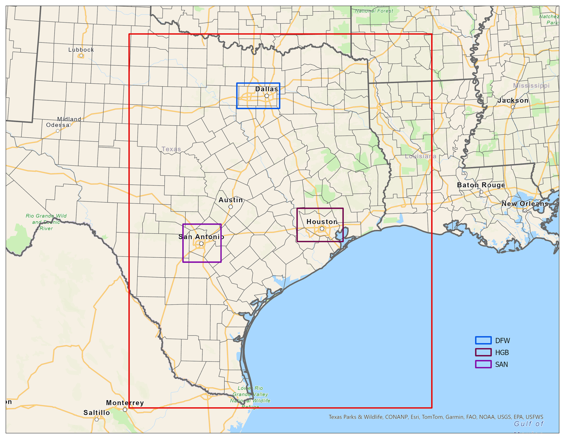
Figure 1 The 4 km (red box) CAMx modeling domain used by TCEQ to model year 2019 in Texas. Data for the DFW, HGB, and SAN box model scenarios were extracted from the TCEQ modeling database for the rectangular regions surrounding these cities.

Daily emissions of NO_X, anthropogenic VOC (AVOC), biogenic VOC (BVOC), and CO for the HGB, DFW, and SAN scenarios are provided in Table S1 in the Supplement. Anthropogenic NO_X (ANO_X) and AVOC emissions for years with available OPE measurements in the Houston area (Table 1) were used to interpolate box model results to measurement years. Since emission inventory methodologies have changed over the time period considered for this study, total ANO_X and total AVOC emissions were used for the interpolation. VOC speciation is therefore constant over all years, consistent with 2019 emission speciation.

Table 1 Anthropogenic NO_X (ANO_x) and anthropogenic VOC (AVOC) emissions from point and non-point sources for Harris County, TX for model year (2019) and years with available aircraft OPE measurements. Emissions data provided by the Texas Commission on Environmental Quality.

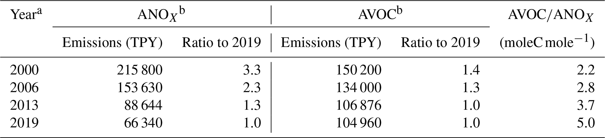
^a Point source emissions are year-specific; non-point source emissions are interpolated from data for 2002, 2005, 2008, 2011, 2014, and 2020. ^b Emission inventory methodologies vary over time period shown.

2.3 Chemical mechanisms

Model simulations used gas-phase chemical mechanisms in CAMx version 7.2 (Emery et al., 2024), specifically the Carbon Bond mechanism versions 6 revision 5 and 7 revision 1 (CB6r5 and CB7r1; Yarwood et al., 2020, 2021), the toxics version of the Statewide Air Pollution Research Center 2007 mechanism (SAPRC07TC; Carter, 2010a, b), and a version of the Regional Atmospheric Chemistry Mechanism version 2 provided by the mechanism developer in September 2021 (RACM2s21; William Stockwell, personal communication, 2021; Goliff et al., 2013). We coordinated with each mechanism's developer to ensure that they are implemented as intended. Coordination is particularly relevant to photolysis reactions and we use cross-section and quantum yield data provided by each mechanism developer, which we implemented into the Tropospheric Ultraviolet and Visible (TUV) radiative transfer model (NCAR, 2025) as a CAMx preprocessor (Ramboll, 2024).

We harmonized treatments of heterogeneous chemistry and iodine to focus on gas-phase reactions that relate O₃ and NO_Z. In CAMx, both CB6r5 and CB7r1 include a compact scheme (16 reactions) for O₃ destruction by oceanic iodine emissions (Emery et al., 2024) which we deactivated by zeroing photolysis frequencies of I₂ and HOI in the chemistry input file for these mechanisms. Ozone destruction by iodine can be several ppb d⁻¹ for coastal locations such as Houston (Tuite et al., 2018). We deactivated the CAMx particle-phase and aqueous-phase chemistry in the chemistry input file for each mechanism. However, hydrolysis of N₂O₅ and ONs remained active for all mechanisms with consistent rate assumptions. With CAMx heterogeneous chemistry turned off, N₂O₅ hydrolyzes to HNO₃ at the bimolecular gas-phase rate (i.e., N₂O₅+H₂O) measured by Wahner et al. (1998) and all ONs hydrolyze to HNO₃ with a lifetime of 12 h derived from the experiments by Liu et al. (2012) and the ambient measurements of Rollins et al. (2013). We note that many ONs likely have shorter hydrolysis lifetimes (Zhao et al., 2023) and the 12 h lifetime used here may be a conservative estimate.

The Supplement lists the reactions of each mechanism (Tables S4, S7, S10 and S13 in the Supplement), their model species (Tables S5, S8, S11 and S14 in the Supplement) and photolysis rates at representative conditions for several zenith angles (Tables S6, S9, S12 and S15 in the Supplement). CB6r5 is the most compact (208 reactions and 80 species) followed by CB7r1 (214 reactions and 86 species), RACM2s21 (372 reactions and 117 species) and SAPRC07TC (567 reactions and 120 species). The major changes from CB6r5 to CB7r1 are a new scheme for isoprene (species ISOP) based on Wennberg et al. (2018), a new terpene scheme based on Schwantes et al. (2020) that separates α-pinene (APIN) from other terpenes (TERP), revised reactions of paraffinic alkoxy radicals (ROR) that better differentiate how aldehyde and ketone formation depend on temperature and O₂ concentration, and less reactive cresol (CRES) and aromatic ring-opening product (OPEN) to reduce reactivity of benzene (BENZ) and toluenes (TOL) in better agreement with SAPRC07. Inorganic reaction rate constants were updated for CB6r5 and carried forward to CB7r1.

The mechanisms rely on different data sources for inorganic reaction rate constants. In general, SAPRC07 uses the Sander et al. (2006) recommendations, CB6r5 and CB7r1 follow Cox et al. (2020), and RACM2s21 uses Burkholder et al. (2019). We conducted a sensitivity test where all mechanisms used the same OH+NO₂ rate constant which reaffirmed the importance of this rate constant to O₃ production.

2.4 Computing OPE with Chemical Process Analysis (OPE-CPA)

Model concentrations (C_i) of species i change with time due to chemistry according to:

$$\begin{array}{}\text{(1)}& {\displaystyle \frac{\mathrm{d}{C}_i}{\mathrm{d}t}}=\sum _n{s}_{i,n}{r}_n,\end{array}$$

where the r_n are rates (dimension concentration/time) of reactions involving species i and the s_i,n are stoichiometric coefficients which must be multiplied by −1 for reactants. The r_n depend on C_i because they are computed as the product of reactant concentrations and the reaction rate constant (or photolysis frequency) for each reaction. Time integration of the coupled equations for C_i and r_n is performed by the CAMx chemistry solver, usually Hertel's enhancement of Euler's method (Hertel et al., 1993). Process analysis captures the r_n at each CAMx time step and accumulates them for output in step with the model output for C_i. These integrated reaction rates can be subsequently analyzed to diagnose chemically interesting quantities (termed process analysis) such as oxidant production rate or oxidant production sensitivity indicators (Tonnesen and Dennis, 2000; Tonnesen and Luecken, 2004). However, these calculations are mechanism specific and can be complex to implement. CPA internalizes these calculations within CAMx to directly output the chemically interesting quantities, which standardizes methodology and is simpler to use.

We use CPA to compute the OPE for model simulations (OPE-CPA) as the ratio of net O₃ production P_n(O₃) to net NO_Z production P_n(NO_Z) from start time t₁ to end time t₂:

$$\begin{array}{}\text{(2)}& \text{OPE-CPA}={\left[{\displaystyle \frac{P_n\left({\mathrm{O}}_{\mathrm{3}}\right)}{P_n\left({\mathrm{NO}}_z\right)}}\right]}_{t\mathrm{1}}^{t\mathrm{2}},\end{array}$$

where net species production rate (P_n) signifies the net effect of chemical production combined with loss, and is computed within CAMx from integrated reaction rates (irr_n) as:

$$\begin{array}{}\text{(3)}& P_{n_i}=\sum _n{s}_{i,n}{\text{irr}}_n,\end{array}$$

We take t₁ as the first hour after sunrise with positive P_n(O₃) and t₂ as hour 15 (15:00–16:00 local time (LT)) which is consistent with flight times that measured OPE near Houston (discussed above) and encompasses hours with maximum O₃ production in our model simulations, as shown below. We used the same t₂ for other cities for comparability. Details of calculating P_n(O₃) and P_n(NO_Z) for each mechanism are provided in the Supplement.

The irr values are local to each CAMx grid cell meaning that they are not directly influenced by model transport (advection and diffusion) or deposition processes. Transport and deposition indirectly affect chemistry by changing species concentrations and therefore can also indirectly affect irr values. Here, CAMx is configured as a 2-box model with the top of layer 1 following the PBL height provided by WRF. The aircraft flights that measured OPE near Houston were conducted within the PBL and therefore comparable to OPE-CPA for our CAMx layer 1. The change in PBL depth between t₁ and t₂ is accounted for when computing OPE-CPA by a weighting factor (${\text{PBL}}_t/{\text{PBL}}_{\text{max}}$):

$$\begin{array}{}\text{(4)}& {\left[\text{OPE-CPA}\right]}_{t\mathrm{1}}^{t\mathrm{2}}={\displaystyle \frac{{\sum }_{t\mathrm{1}}^{t\mathrm{2}}\left(\frac{{\text{PBL}}_t}{{\text{PBL}}_{\text{max}}}\right)P_n\left({\mathrm{O}}_{\mathrm{3}}\right)}{{\sum }_{t\mathrm{1}}^{t\mathrm{2}}\left(\frac{{\text{PBL}}_t}{{\text{PBL}}_{\text{max}}}\right)P_n\left({\mathrm{NO}}_z\right)}},\end{array}$$

where PBL_max is the largest PBL depth between t₁ and t₂. This weighting considers that a deeper PBL contains more air mass and therefore contributes proportionately more to net species production within the time period analyzed. We applied Eq. (4) as a post-processing step using hourly-averaged P_n obtained from CPA and the PBL depth from WRF.

3 Results and discussion

3.1 OPE measurements

We focus on the OPE-plot estimates for two reasons. First, more estimates are available from the OPE-plot method than the plume integration or plume center-edge methods. Second, CSS models require a chemical mechanism, and thus the OPE estimates depend on the mechanism employed. This adds uncertainty to the OPE estimates, which is difficult to assess because different mechanisms have been used in different modeling studies and all the mechanisms used are older than those being compared in this work.

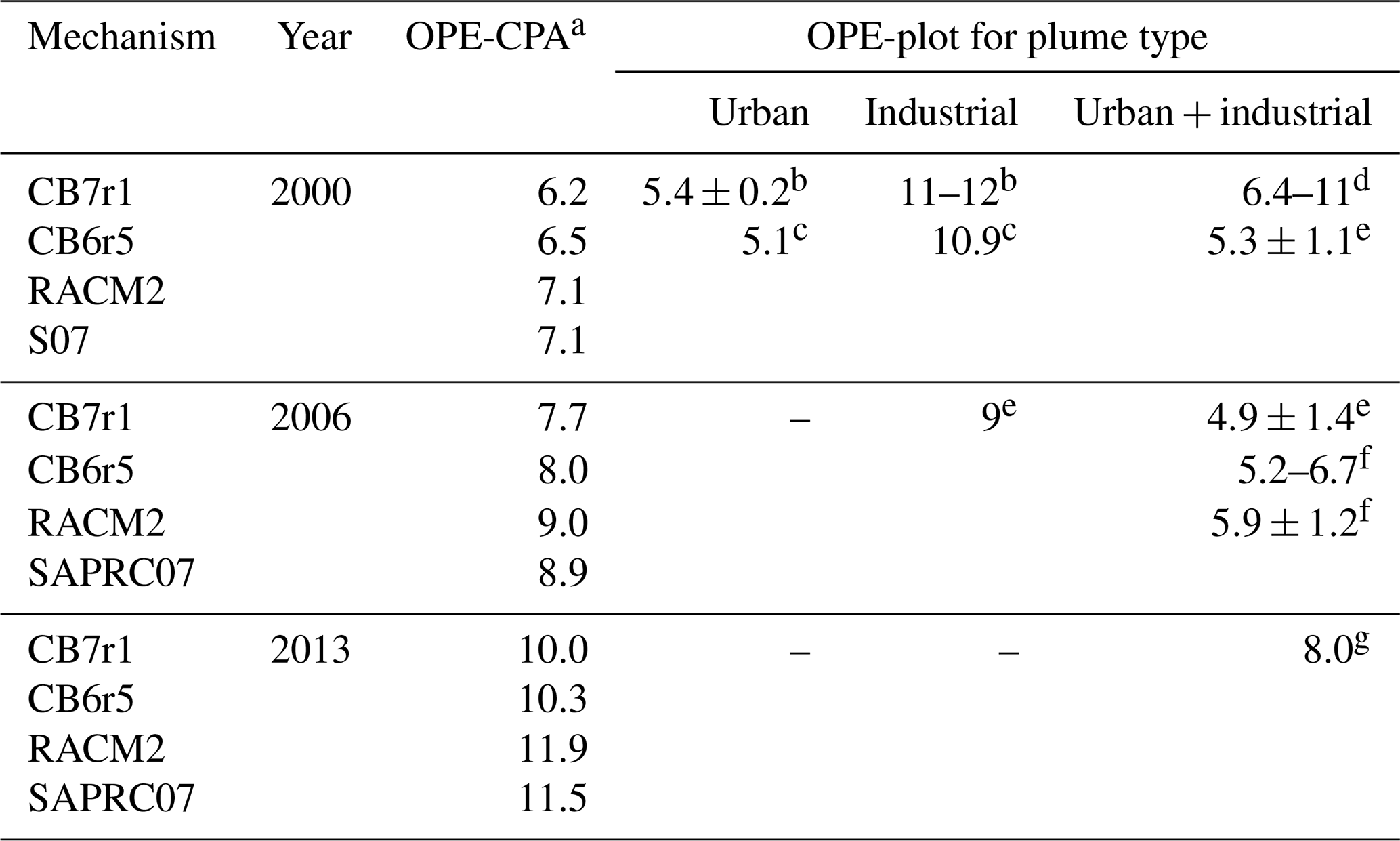
Table 2 gives OPE-plot estimates determined from aircraft measurements in Houston, Texas in 2000, 2006, and 2013. The daily time period of the measurements differs from study to study but generally contains the early to middle-afternoon hours with 15:00 or 16:00 LT being the endpoint of most periods. The OPE estimates for the industrial plumes in Houston in 2000 (∼11) are about twice as large as those for the urban plumes (∼5). This is attributed to large emissions of highly reactive VOCs (HRVOCs) from the petrochemical industry increasing OPE by forming O₃ efficiently in downwind plumes (Ryerson et al., 2003; Daum et al., 2003). The coalesced industrial and urban plumes in 2000 had OPEs similar to those of the urban plumes that year. The OPEs for the coalesced industrial and urban plumes were essentially the same in 2006 as in 2000, which may be due to offsetting effects of emissions reductions. There were large reductions in Houston's NO_X emissions from 2000–2006 and in HRVOC emissions from petrochemical facilities (Zhou et al., 2014) due to the HRVOC Emissions Cap and Trade (HECT) Program (TCEQ, 2025). The reduction in HRVOC emissions should reduce OPE, but a reduction in emissions and atmospheric concentrations of NO_X generally increases OPE (Kleinman et al., 2002; Mazzuca et al., 2016; Henneman et al., 2017). The OPE for the industrial plume in 2006 is about 20 % smaller than the OPEs for the industrial plumes in 2000, consistent with the reduced HRVOC emissions. The Houston coalesced industrial and urban plumes in 2013 had an OPE of 8, which is 35 %–60 % larger than the estimates for 2006. The increase in 2013 might be due to the continuing NO_X emission reductions in Houston.

Table 2 Estimates of net OPE from aircraft measurements in Houston, TX.

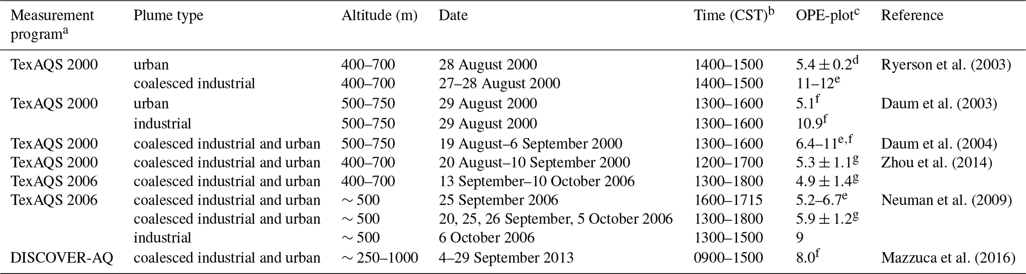
^a TexAQS = Texas Air Quality Study; DISCOVER-AQ = Deriving Information on Surface Conditions from Column and Vertically Resolved Observations Relevant to Air Quality. ^b Approximate time period of the measurements based on information in the references. ^c O₃ used to determine OPE unless otherwise indicated. ^d Uncertainty from the linear fit of O₃ to NO_Z data. ^e Range for multiple transects/plumes. ^f ${\mathrm{O}}_{\mathrm{X}}={\mathrm{O}}_{\mathrm{3}}+{\mathrm{NO}}_{\mathrm{2}}$ used instead of O₃
^g Average over multiple transects.

The OPE-plot estimates in Table S2 in the Supplement from the regional INTEX-NA and SEAC4RS flights over the southeast US (14 and 17 respectively) are significantly larger than all the estimates for Houston. This difference likely results from the lower NO_Z concentrations measured in the regional flights than in the Houston flights. The smaller NO_Z concentrations could be due to greater dilution of NO_X emissions by background or rural air or greater deposition of NO_Z, which would increase the OPE estimates. The OPE estimates from DISCOVER-AQ for the Baltimore urban area in 2011 (8.4±4.1) and the estimates for for New York City (9±4) and Chicago (6±3) in 2023 from AEROMMA are similar to those for the Houston coalesced industrial and urban plume in 2013 (8.0). However, the NO_X concentrations and also likely the VOC concentrations vary among these urban plumes, and consequently the similar OPE values do not imply that the chemistry is similar in the plumes. Again, increased NO_X and increased VOC emissions can have opposing effects on OPE that cancel.

The OPE-plot estimates for many surface sites in Table S3 in the Supplement are also larger than the estimates for Houston in Table 2. This is expected for rural sites because the NO_X or NO_Z concentration is generally smaller than in Houston, leading to larger OPE estimates. At Whiteface Mt., for example, the median NO_X concentration was only 0.2 ppb. Similarly, the urban and suburban SEARCH sites have smaller NO_Z concentrations than the Houston measurements. The OPE estimates for Durham and Flushing are comparable to that for Houston in 2013, consistent with similar NO_Z concentrations at these locations.

The OPE values in Tables 2, S2 and S3 have additional uncertainties that are not reflected in the shown uncertainties. The most important is the amount of NO_Z species, particularly HNO₃, deposited prior to the measurements. If this deposition is significant, OPE-plot is an upper limit to the OPE determined by the chemistry alone. Also, OPE-plot may not represent O₃ formation in a single air parcel because the measurements may sample different air parcels containing emissions from different sources or sample an air parcel that is a mixture of multiple air parcels with different photochemical ages. These complications can introduce significant scatter and nonlinearity into the O₃ vs. NO_Z relationship that alters the linear regression of the data. OPE-plot from surface data is more strongly influenced by these uncertainties than OPE-plot from aircraft flights because analyses of surface data usually combine data from many days and different air parcels whereas flight transects focus on a specific air parcel over a short time period, and surface measurements are more likely to be affected by HNO₃ deposition.

3.2 Model base cases and O₃ response surfaces

Four chemical mechanisms were evaluated using results from the CAMx 2-box model scenarios. We focus on the Houston (HGB) scenario due to the availability of OPE measurements at this location and investigate mechanism differences in O₃, NO_Z (${\mathrm{HNO}}_{\mathrm{3}}+\mathrm{ONs}+\mathrm{PANs}$), and NO_Y (NO_Z+NO_X), which are most relevant to OPE. Results from the other model locations, DFW and SAN, are provided in the Supplement for comparison.

Time series of hourly average O₃ and NO_Z concentrations over the 5 d model period are shown in Fig. 2. The diurnal trends for both species are similar between mechanisms. O₃ increases throughout the day and peaks in the late afternoon, whereas NO_Z increases throughout the day and overnight, peaks in the early morning, and decreases sharply as the PBL grows. The buildup in O₃ concentration over the first two days results from carryover of O₃ via the residual layer. The accumulated O₃ in the residual layer (layer 2 of the model) is ventilated to background air and/or entrained into the PBL (layer 1) and the concentration stabilizes after 2 d. The minimum O₃ concentration for days 2 through 5 is about 65 ppb, which is greater than typically seen in urban measurements. This is likely due to the emissions averaging performed in the model which includes areas outside of the urban core (see Fig. 1), leading to weaker NO_X titration effects. CO (Fig. S2 in the Supplement) shows a similar trend as O₃. Day 1 is considered model spin-up and we focus on model days 2 through 5 so that initial conditions have minimal importance and emissions have maximum importance in the simulations.

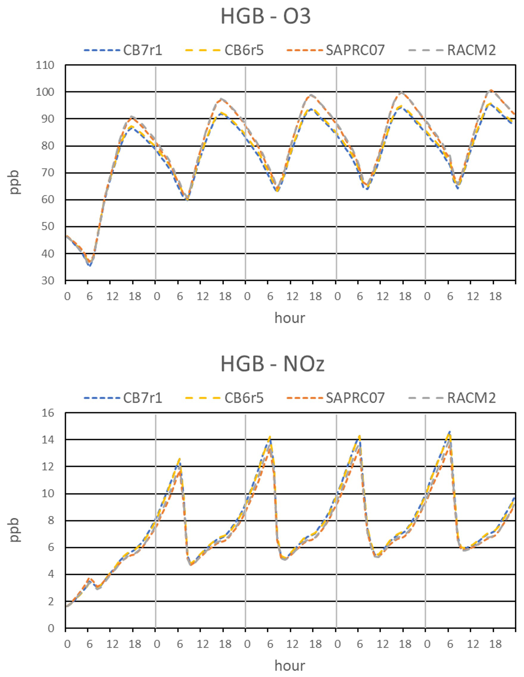
Figure 2 Time series of O₃ and NO_Z (${\mathrm{HNO}}_{\mathrm{3}}+\mathrm{ONs}+\mathrm{PANs}$) simulated by four chemical mechanisms for the HGB box model scenario, shown in local time from 3–7 September 2019.

RACM2 and SAPRC07 predict higher daytime O₃ compared to CB6r5 and CB7r1, by about 5 ppb at the time of peak O₃ in late afternoon. The DFW model scenario (Fig. S3 in the Supplement) shows similar results but O₃ concentrations in the SAN scenario (Fig. S4 in the Supplement) agree closely between mechanisms. NO_X concentrations are higher at HGB and DFW, indicating that RACM2 and SAPRC07 may produce O₃ more efficiently in high NO_X environments. We investigated the importance of the $\mathrm{OH}+{\mathrm{NO}}_{\mathrm{2}}={\mathrm{HNO}}_{\mathrm{3}}$ reaction to O₃ differences by performing a sensitivity test where all mechanisms use the same rate constant. The RACM2 rate was changed to the Sander et al. (2006) recommendation used in CB6r5, CB7r1, and SAPRC07. Note that the NASA recommended rate for the $\mathrm{OH}+{\mathrm{NO}}_{\mathrm{2}}={\mathrm{HNO}}_{\mathrm{3}}$ reaction remained unchanged from 2006–2019. Results of this test for HGB are shown in Fig. S5 in the Supplement. RACM2 OH and O₃ decrease and become more like CB6r5 and CB7r1, indicating that the difference in rate is a significant contributor to the higher RACM2 OH and O₃. There is also a 6 % difference between current Sander et al. (2006), Burkholder et al. (2019) and Cox et al. (2020) recommendations which is a meaningful uncertainty that should be resolved (Amedro et al., 2020).

All mechanisms produce similar levels of daytime NO_Z, with slightly higher values from CB6r5 and CB7r1. NO_Y concentrations are also similar between mechanisms but there are some differences in composition. NO_Y composition at 15:00 LT on each model day is shown in Fig. 3 for each mechanism. HNO₃ is the dominant NO_Y species, highlighting the importance of the OH + NO₂ reaction in NO_Z net production, P_n(NO_Z), for all mechanisms. OH and NO₂ concentrations (Fig. S2) are highest from RACM2, resulting in slightly higher HNO₃. While NO₂ is similar among the other three mechanisms, SAPRC07 has lower OH and consequently lower HNO₃. As noted above, the rate constants for the OH+NO₂ reaction also vary between mechanisms, contributing to differences in HNO₃. Concentrations of total ONs and peroxyacyl nitrates (PANs) vary between mechanisms. ON is lowest from RACM2 and this nitrogen is shifted to other NO_Y species resulting in higher NO, NO₂, and PANs. Daytime ONs from RACM2 also remain relatively constant whereas the other mechanisms show increasing concentration throughout the day, consistent with RACM2 recycling more ONs to NO_X than other mechanisms. Daytime PANs are highest from SAPRC07 and lowest from CB6r5 and CB7r1. Higher concentrations in SAPRC07 are due to higher levels of the precursor acetyl and acyl radicals involved in the formation of PANs. These radical concentrations are influenced by VOC oxidation and radical chemistry, in addition to thermal decomposition of PANs. Lower PANs concentrations in CB6r5 and CB7r1 are due to lower peroxyacyl radical concentrations. Daytime NO is highest from RACM2 due to higher daytime NO₂ and rapid interconversion via the Leighton cycle (Leighton, 1961). Higher NO contributes to higher OH and lower HO₂ for RACM2 due to the $\mathrm{NO}+{\mathrm{HO}}_{\mathrm{2}}={\mathrm{NO}}_{\mathrm{2}}+\mathrm{OH}$ reaction. The higher OH for RACM2, which is consistent across all three locations, will influence how many pollutants are removed in RACM2 compared to the other mechanisms.

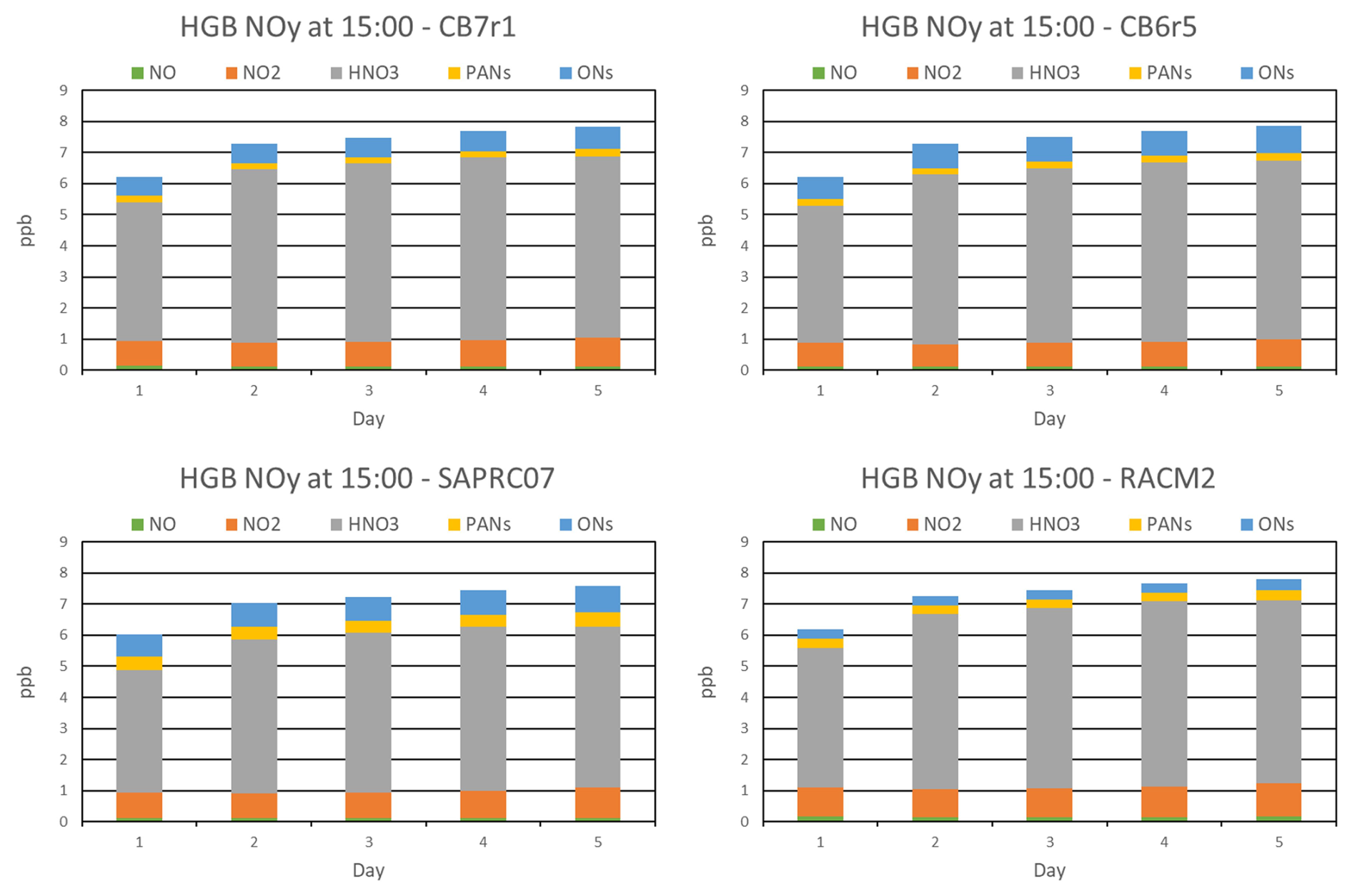
Figure 3 NO_Y composition simulated by four chemical mechanisms for the HGB box model scenario, shown at 15:00 LT for each modeled day.

In addition to base case simulations, we investigated how varying ANO_X and AVOC emissions impact O₃ and OPE-CPA by performing a matrix of 196 box model simulations. Scale factors of 0.1–5.0 were applied to the base emissions and Fig. 4 shows resulting O₃ response surface plots (for O₃ at 15:00 LT) for the four mechanisms. The base cases are at NO_X and VOC scale factors of (1,1) and are in a NO_X limited regime since O₃ reduces more rapidly with NO_X reductions than with VOC. As in the base case, RACM2 and SAPRC07 show higher O3 across all emission scales, but all mechanisms show a similar response shape. In particular, the location of the “ridgeline”, which separates NO_X limited from VOC-limited conditions, is similar between mechanisms. Scale factors below 1.0 are relevant to near-term air quality planning purposes since existing strategies are expected to reduce emissions, particularly of NO_X. For all mechanisms, O₃ formation in this range is in a NO_X limited regime indicating that all mechanisms find NO_X emission reductions will be more effective than VOC reductions for HGB as well as DFW and SAN (see the Supplement).

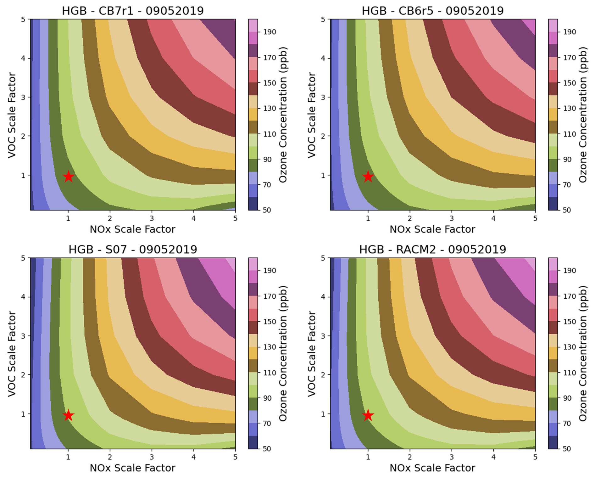
Figure 4 O₃ response surface plots at varying anthropogenic VOC and anthropogenic NO_X emissions for four chemical mechanisms, with the star indicating the base case. O₃ at 15:00 LT for day 3 (5 September 2019) of the HGB box model scenario is shown. Other modeled days show similar O₃ responses.

Overall, our results show relatively good agreement among the mechanisms consistent with Derwent (2017, 2020) and Shareef et al. (2022) but different from the lower O₃ formation found by Chen et al. (2024) for CB6r2. The reason for the low O₃ formation with CB6r2 in the Chen et al. (2024) work is unclear.

3.3 OPE-CPA comparison

OPE-CPA was computed from the matrix simulations using the method described in the Sect. 2.4. Transects of OPE-CPA at varying anthropogenic NO_X and VOC scaling factors are presented in Figs. 5 and 6, respectively. In general, OPE-CPA for each of the mechanisms responds similarly to varying emissions, increasing as VOC increases and decreasing as NO_X increases. Note that even at the lowest AVOC scaling factor of 0.1, O₃ chemistry is not strongly VOC-limited, but is instead in the transition between NO_X and VOC-limited conditions, as can be seen in Fig. 4. At high VOC $/$ NO_X ratios, OPE-CPA can peak or plateau but this behavior is not consistent from day to day or among mechanisms due to differences in concentrations and chemistry differences between the mechanisms. This aligns with inconsistencies in measurements (Ninneman et al., 2017; Blanchard and Hidy, 2018) and prior modeling studies (Kleinman et al., 2002; Mazzuca et al., 2016; Henneman et al., 2017), some of which observed a peak or plateau and others did not. Regardless of OPE behavior, however, O₃ in our simulations continues to decrease as NO_X decreases (Fig. 4).

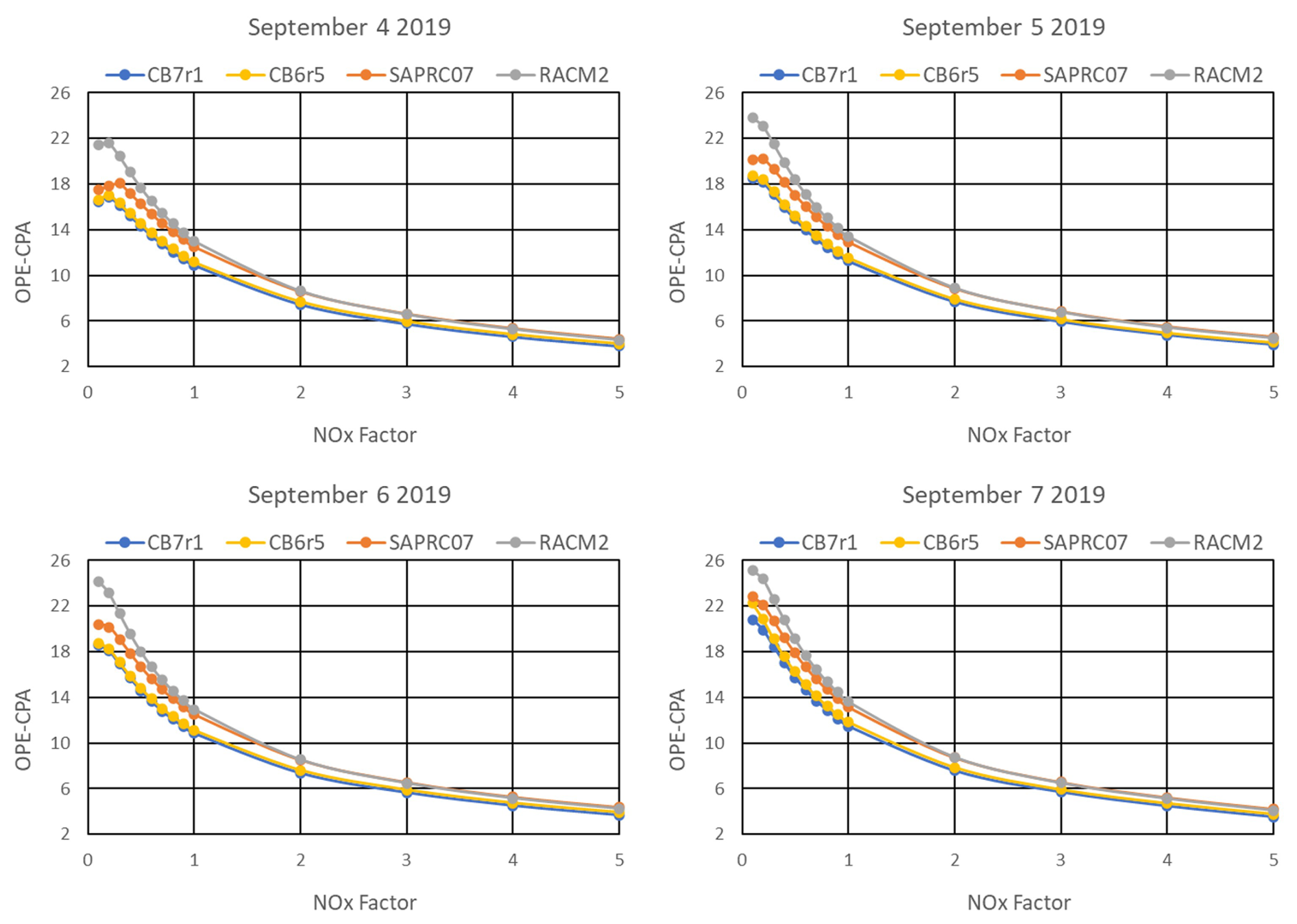
Figure 5 OPE-CPA calculated with t₂=15:00 LT at varying anthropogenic NO_X emission scaling factors and base VOC emissions, simulated by four chemical mechanisms for the HGB box model scenario.

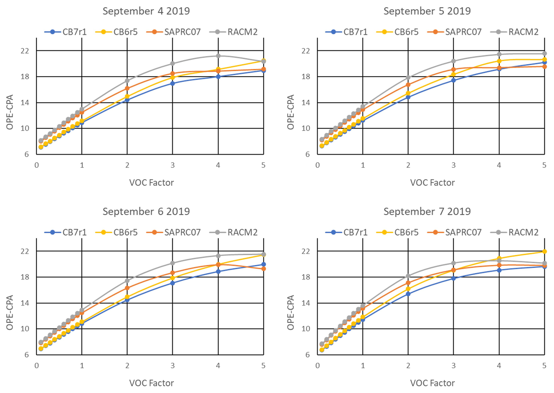
Figure 6 OPE-CPA calculated with t₂=15:00 LT at varying anthropogenic VOC emission scaling factors and base NO_X emissions, simulated by four chemical mechanisms for the HGB box model scenario.

RACM2 consistently has the highest OPE-CPA across all NO_X and VOC scales and CB7r1 has the lowest. As discussed in the previous section, HNO₃ is the largest component of NO_Z and NO_Y (Fig. 3), so OH+NO₂ dominates P_n(NO_Z). The slower OH+NO₂ rate in RACM2 contributes to the higher OPE-CPA, as is evident from our sensitivity test which normalized the rate among all four mechanisms. When the RACM2 rate was adjusted to match the other mechanisms, OPE-CPA decreased by about 7 % in the HGB base case simulations, putting it between values for SAPRC07 and CB7r1. OPE-CPA also decreased across all NO_X scaling factors (Fig. S14 in the Supplement) but is still higher than the other mechanisms at low NO_X on all model days.

Another factor that may play a role in the OPE-CPA differences is NO_X recycling. Differences between mechanisms are largest at high VOC $/$ NO_X ratios (NO_X factor<1 in Fig. 5 and VOC factor>1 in Fig. 6) where O₃ formation is strongly limited by NO availability and NO_X recycling becomes more important. The mechanism differences at NO_X factor<1 are particularly important to note since this may be relevant to air quality planning. RACM2 allows all ONs to recycle nitrogen to NO_X but the other mechanisms include ON species (XN in SAPRC07 and NTR2 in CB6r5 and CB7r1) which do not recycle. Gas-phase mechanisms that resolve ON speciation in more detail provide greater opportunity for atmospheric models to resolve the influences of heterogeneous chemistry and deposition on ON lifetime and fate. Among the mechanisms discussed here, RACM2 resolves ONs the least and CB6r5 and CB7r2 resolve ONs the most. The differences in ON speciation and NO_X recycling may contribute to higher OPE-CPA for RACM2 under NO_X-limited conditions.

Table 3 provides a comparison of OPE-CPA to OPE-plot calculated from measurements near Houston. Model results were interpolated to measurement years using the emissions trends shown in Table 1. We assume model emissions represent a combination of general urban and industrial emissions so that model comparisons to urban + industrial measurements are most appropriate. OPE-CPA is similar to the urban + industrial measurements in 2000 but greater than those in 2006 and 2013. One uncertainty in the comparison relates to how VOC emissions have changed from 2000–2019. In particular, emissions of highly reactive VOCs (HRVOCs) declined by 40 % from 2000–2006 due to targeted reductions from industrial sources (Zhou et al., 2014) and likely have remained lower through 2019. However, our model VOC speciation is constant over all years and representative of 2019, so changes in HRVOCs are not captured. Since higher HRVOC concentrations are expected to increase OPE, our OPE-CPA may be an underestimate for the measurement years, particularly for 2000. The higher OPE in industrial plumes in Table 3 are likely due to increased levels of HRVOCs and/or higher VOC $/$ NO_X ratios. 3D modeling is better suited than box modeling to further investigate how VOC $/$ NO_X ratios vary between plumes.

Table 3 Comparison of modeled to measured OPE for Houston.

^a Calculated with t₂=15:00 LT and averaged over model days 2–5 (4–7 September 2019); Harris County emission trends are used to interpolate CPA-OPE from model year (2019) to measurement years (2000, 2006, 2013). ^b Ryerson et al. (2003); ^c Daum et al. (2003); ^d Daum et al. (2004); ^e Zhou et al. (2014); ^f Neuman et al. (2009); ^g Mazzuca et al. (2016).

Another important difference between OPE-CPA and OPE-plot is the influence of NO_Z deposition. Our OPE-CPA is only indirectly affected by deposition (see Sect. 2.4) but OPE-plot is directly influenced by deposition, although with less impact for these aircraft measurements than for surface measurements as discussed above. Because of this, comparison between OPE-CPA and OPE-plot is difficult. Still, considering the range in OPE-plot, OPE-CPA values are reasonable and the differences may not be significant given the uncertainties. Insufficient measured OPE data over time also make it difficult to determine whether trends are consistent.

The impact of NO_X reductions on OPE-CPA and O₃ are shown in Table 4. In model runs where ANO_X emissions are reduced by 50 %, OPE-CPA increases by 32 %–38 % depending on the mechanism, O₃ concentration at 15:00 LT decreases by 14 %–17 %, and daily net O₃ production (calculated as maximum minus minimum O₃) decreases by 57 %–65 %. The decrease in O₃ concentration is smaller than that for O₃ production due to the contribution of background O₃. The increase in OPE-CPA is noticeably larger for RACM2, consistent with the transects shown in Fig. 5, and corresponds to the smallest decrease in daily net O₃ production as NO_X is reduced. The higher OPE-CPA for RACM2 for both the base and 50 % ANO_X cases corresponds to higher O₃ concentration and production. SAPRC07 has the smallest relative change in OPE-CPA but the largest change in O₃. The fact that each mechanism shows a similar OPE dependence on NO_X emissions and predicts similar reductions in O₃ is reassuring from a regulatory modeling perspective.

Table 4 Comparison of simulated CPA-OPE and O₃ (at 15:00 LT) and daily net O₃ production from four chemical mechanisms for HGB between base emission scenario and 50 % anthropogenic NO_X (ANO_X) emission scenario.

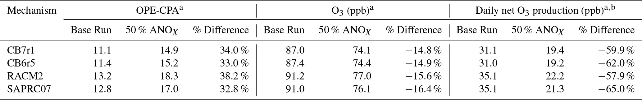
^a Averaged over model days 2–5. ^b Calculated as the difference between the daily maximum and daily minimum concentration, which occurred respectively at 18:00 and 09:00 LT for all mechanisms.

OPE-CPA increases as NO_X decreases but, counterintuitively, O₃ still decreases (see Figs. 4 and 5). Also, the percent increase in OPE-CPA for a 50 % reduction in ANO_X is about twice as large as the percent O₃ decrease (Table 4). P_n(O₃) is impacted by factors other than OPE (e.g., VOC oxidation rate) which also depend on NO_X. The difference in the relative changes of OPE and O₃ indicate that using OPE to predict O₃ response to NO_X emissions would be an over-simplification that will tend to over-state O₃ reductions. This may be especially true at low NO_X where the mechanisms have the largest variation in OPE-CPA.

As discussed in the Sect. 2, OPE-plot is derived from a linear relationship between O₃ and NO_Z, which depends on NO_X. OPE-CPA, on the other hand, varies nonlinearly with NO_X, as seen in Fig. 5. It is unclear why a linear relationship of O₃ and NO_Z is observed in measurements despite a nonlinear relationship between P_n(O₃) and P_n(NO_Z) (Kleinman et al., 2002). Additional studies which focus on the influence of plume dilution, composition of background air, and variations of VOC $/$ NO_X within plumes are needed to explain why OPE-plot and OPE-CPA behave differently. For example, by conducting 3D simulations with finely resolved grids and emission data, sub-hourly OPE-plot and OPE-CPA computed along pseudo aircraft trajectories could be compared.

4 Conclusions

4.1 Summary of results and uncertainties

We performed CAMx 2-box model simulations with four widely used chemical mechanisms (CB6r5, CB7r1, RACM2, and SAPRC07) and computed OPE using chemical process analysis (OPE-CPA). In general, we found relatively good agreement between the mechanisms for O₃, NO_Z, NO_Y, and OPE-CPA at all three Texas locations. There was better O₃ agreement at SAN compared to HGB and DFW, indicating that mechanism differences in O₃ production are greater in high NO_X environments. Higher values of O₃, OH, and OPE-CPA from RACM2 are partially due to a slower OH+NO₂ rate constant compared to the other mechanisms. OH+NO₂ is important to O₃ chemistry and dominates P_n(NO_Z) so it plays a key role in OPE. Sensitivity tests for HGB showed better agreement when a consistent rate was applied for all mechanisms. Different rate constant recommendations from IUPAC and NASA can contribute to overall mechanism uncertainty, particularly via the important OH+NO₂ reaction, demonstrating that new rate constant measurements are valuable (e.g., Rolletter et al., 2025; Amedro et al., 2020) together with updated rate constant recommendations. It is noteworthy that uncertainties in extensively studied inorganic reactions continue to be among the larger known uncertainties in chemical mechanisms.

We investigated how varying NO_X and VOC emissions impact O₃ and OPE-CPA and found similar responses among all mechanisms. O₃ response surfaces show that the base emissions scenarios are in a NO_X limited regime for all three locations. OPE-CPA is inversely related to NO_X and differences between mechanisms are greatest at high VOC $/$ NO_X ratios. In addition to the OH+NO₂ rate contributing to higher RACM2 OPE-CPA, the treatment of NO_X recycling, which varies between mechanisms, may also play a role. The increase in OPE-CPA at low NO_X occurs even as O₃ production and concentration decrease. The relative changes in OPE-CPA and O₃ to varying NO_X are notably different, e.g., the OPE-CPA percent increase is 2 times larger than the O₃ percent decrease at 50 % ANO_X, which highlights the difficulty of using OPE to predict O₃ response to NO_X. OPE-CPA and O₃ show anti-correlated responses to varying VOC $/$ NO_X ratios and there is not a linear relationship between them which prevents OPE-CPA from being a simple predictor of O₃ production.

The fact that all mechanisms show a similar dependence of OPE and O₃ to NO_X emissions, however, does indicate that OPE-CPA can be used to compare mechanisms. Unlike Maximum Incremental Reactivity (MIR) factors though, which can be used to characterize O₃ formation under specific VOC-limited conditions, there is no obvious emission condition to compare OPE-CPA. We recommend further studies to investigate whether a suitable condition (perhaps, for example, 50 % of peak OPE) exists to better utilize OPE-CPA as a comparison factor. This is especially important due to the limitations of MIR for NO_X-limited conditions, which are common in many regions in the US and relevant for air quality planning purposes.

OPE-CPA from the HGB simulation was also compared to available measurements (OPE-plot) in the Houston area. We focused on aircraft OPE measurements since surface measurements are subject to large uncertainties from deposition. Comparison to DFW and SAN simulations were not possible due to lack of measurements. While OPE-CPA was in relatively good agreement with OPE-plot, there are aspects which make comparison difficult, including uncertain VOC speciation and impacts of dilution and NO_Z deposition. The limited number of OPE measurements also restrict our ability to make conclusions about OPE trends over time. Additional aircraft based OPE measurements downwind of previously studied locations would be useful to test mechanism response to emission reductions, and speciated VOC measurements would help characterize the reactivity of emissions. Clear reporting of the time of day for OPE measurements would also reduce uncertainty in comparisons between OPE-CPA and OPE-plot.

4.2 Potential future work

Applying OPE-CPA in 3D simulations is feasible and complementary with other methods used to probe 3D model simulations, such as sensitivity analysis. CPA can reveal spatial variations in chemical conditions between grid cells that are less apparent using sensitivity analysis due to the influence of transport. 3D simulations of urban plumes using a fine horizontal grid resolution could investigate why measured OPE is often stable within a plume even when subject to varying NO_X emissions. Comparison of OPE-CPA and OPE-plot along pseudo aircraft transects in the same simulated plume would help us better understand if the two provide similar estimates of OPE. In contrast to a box model, 3D simulations may also place different emphasis on pollution carryover versus same day chemistry and the importance of PANs and ONs versus HNO₃. On a regional scale, the difference in ON and PAN chemistry between mechanisms may lead to differences in O₃ production if increased ON and PAN levels allow NO_Y to be transported away from local emission sources and returned as NO_X via photochemical reactions.