Drop clustering and drop size correlations from holographic imagery suggest cloud droplet spectral broadening via entrainment-mixing

The question of how droplets rapidly grow large enough to initiate collision-coalescence has persisted for decades. Many theories explaining the production of sufficiently large drops (i.e., those in the “bottleneck” size range; ∼ 25–50 µm diameters) involve drop clustering on millimeter scales.

A novel method is introduced to evaluate drop clustering trends particle-by-particle (i.e., the number/proximity of neighboring drops for given droplets; defined as drop clustering fields) which are diagnosed relative to drops within their shared drop environments – in contrast to previous studies which diagnose drop clustering of defined sample volumes, or in terms of absolute length scales. Specifically, this study evaluates the statistical likelihood that drops of a given size are associated with either a significant number of neighboring drops, or are significantly isolated from neighboring drops.

Observations are acquired from the HOLODEC during the Cloud System Evolution in the Trades campaign, which sampled subtropical marine clouds. The HOLODEC measures drop size distributions and the 3D spatial coordinates of droplets. Results show drops within the bottleneck size range (diameters of ∼ 25–50 µm) are most likely to be significantly isolated from neighboring drops. This “isolated large drop trend” is primarily observed at subsaturated conditions, suggesting entrainment is the contributing factor. Holograms associated with this trend are more likely to have broader drop size distributions, larger maximum drop sizes and overly regions where precipitation reaches the lowest altitudes from the sampled cloud, suggesting entrainment-mixing drop size distribution broadening is a relevant precipitation-initiation mechanism.

1 Introduction

Explanations for the rapid production of precipitation in warm clouds (e.g., Rauber et al., 2007; Saunders, 1965) have eluded researchers for decades, resulting in numerous theories. Condensational growth rates of droplets to diameters (D) of ∼ 20 µm is well understood, and collision-coalescence is well-evidenced for producing drizzle/rain size drops with those significantly larger than 20 µm (Lamb and Verlinde, 2011). However, for the initiation of collision-coalescence to occur and produce precipitation, drops must first exceed sizes much larger than 20 µm (e.g., Jonas, 1996). The range of drop sizes constituting this “gap” is often termed the “bottleneck” size range, and the production of these drops has remained uncertain for decades. Proposed mechanisms producing drops within the bottleneck size range include but are not limited to the presence of giant cloud condensation nuclei (e.g., Woodcock, 1953; Blyth et al., 2003; Dziekan and Pawlowska, 2017; Dziekan et al., 2021), direct long wave cooling of droplets by emission of thermal infrared radiation near cloud top (Zeng, 2018), inhomogeneous mixing via entrainment (Baker et al., 1980) and various mechanisms related to turbulence (e.g., Chandrakar et al., 2024; Pinsky and Khain, 2002; Siebert and Shaw, 2017; Lu et al., 2018).

Additional growth mechanisms involve drop clustering (i.e., positive spatial correlations between drops) in various manners (e.g., Shaw et al., 1998; Bodenschatz et al., 2010; Madival, 2019). Drop clustering is suspected to occur in varying cloud types given sufficiently large Reynolds numbers as evidenced by in situ observations (e.g., Dodson and Small Griswold, 2019; Larsen et al., 2018; Dodson and Small Griswold, 2022; Bateson and Aliseda, 2012; Kostinski and Shaw, 2001; Glienke et al., 2020), which is a consequence of processes such as inertial clustering and entrainment-mixing (Beals et al., 2015; La et al., 2022). Previous in situ observation studies differ in their conclusions about correlations between drop clustering and drop sizes (e.g., Glienke et al., 2020; Marshak et al., 2005; Small and Chuang, 2008; Thiede et al., 2025). These and other observational studies vary in their usage of instrumentation, spatial scale analysis as well as methods for diagnosing/quantifying the degree of drop clustering.

However, to the authors' knowledge all previous studies have related drop sizes to an “absolute” measure of drop clustering (i.e., diagnosing the clustering of drop systems within sample volumes and/or in terms of absolute length scales), rather than relating drop sizes to the drop clustering defined relative to the drop environments. Comparing drop systems which have been diagnosed as significantly clustered with “non-clustered” drop systems may introduce external biases associated with the two system types (e.g., drop systems are more likely to be clustered at cloud top; Baker, 1992; Dodson and Small Griswold, 2019). It is also plausible that analyzing absolute length scales fails to relate individual drops to small scale features having a variety of spatial scales (e.g., microscale vortices, supersaturation fields, etc.). Additionally, different biases are associated with different drop clustering metrics and counting statistics of droplets can often be insufficient for obtaining robust clustering diagnoses of individual sample volumes (Baker and Lawson, 2010; Larsen et al., 2018; Shaw et al., 2002). These conditions motivated this study to relate drop sizes directly to the degree of “clustering” around individual drops, where the clustering is diagnosed relative to the clustering of their respective drop systems (i.e., sample volumes).

We determine the likelihood that drops of a given size will have a significantly high number of drops surrounding them as well as likelihoods that they are significantly isolated from neighboring drops. Section 2 introduces the instrumentation used in this study and discusses the individual drop clustering diagnosis method. Section 3 outlines two types of analysis performed in this study: (1) determining the relation of drop size to individual drop clustering and (2) correlating individual drop clustering trends with other parameters. Section 4 provides results and Sect. 5 includes further discussion of the findings. Section 6 provides concluding remarks.

2 Instrumentation and methodology

2.1 Instrumentation and field measurements

Data is taken from the National Science Foundation (NSF)/National Center for Atmospheric Research (NCAR) Cloud System Evolution in the Trades (CSET) campaign, which consisted of 16 research flights targeting the stratocumulus to cumulus transition over the Northeastern Pacific (Albrecht et al., 2019) using the NSF/NCAR G-V aircraft. The standard flight plan called for repeated situ sampling patterns, each of which included level legs below-, in- and above-cloud and sawtooth legs across cloud top.

This study primarily relies on observations from the Holographic Detector for Clouds (HOLODEC), which acquires particle size distribution information for constant sample volumes of ∼ 13 cm³ at a rate of 3.3 Hz (Fugal and Shaw, 2009). For flight speeds within regions relevant to this study (∼ 130 m s⁻¹), this results in samples obtained every ∼ 40 m. The HOLODEC measurements provide drop size distribution information of drops with diameters from about 6–1000 µm, as well as the 3D spatial coordinates of the drops. The drop clustering methodology (described in Sect. 2.2) is applied to the HOLODEC measurements.

Measurements acquired from other instruments are collocated to HOLODEC measurements, and are all reported at 1 Hz resolution (∼ 130 m resolution) unless specified otherwise. This includes temperature and water vapor measurements to derive relative humidity (RH), which are acquired from the Rosemount temperature probe and Vertical-Cavity Surface Emitting Laser (VCSEL) hygrometer (Zondlo et al., 2010). The combined uncertainties from the Rosemount temperature probe and VCSEL at the temperature range of observations in this study are expected to result in an RH uncertainty of ∼ 5 %. Because of differences in the sampling rates, 3 or 4 holograms are identified with the temperature and RH measurements, and this may introduce some uncertainty into the analysis. A W-band HIAPER Cloud Radar (HCR) having a 0.5 Hz resolution is also utilized to identify the lowest altitudes of condensate/precipitation in the presence of rain/drizzle. This is possible since the HCR is nadir-pointing for in-cloud flight legs. The lowest condensate/precipitation echoes are defined as the lowest range gate from the aircraft having reflectivity exceed −60 dBZ (no lower clouds or fog are considered). This is to explore how HOLODEC measurements correspond with subsiding condensate. Although no efforts are made to distinguish between precipitation and cloud base, the frequency of virga associated with stratocumulus clouds from CSET is predicted to be ∼ 80 % (Schwartz et al., 2019).

Although the HOLODEC data were processed for all research flights, there is limited data availability since only a few flight legs had relatively long durations in-cloud (shown below). Observations are also limited to level flight legs due to possible measurement biases and consistency with previous studies (Glienke et al., 2017, 2020; La et al., 2022; Larsen et al., 2018; Larsen and Shaw, 2018). Table 1 shows flight legs from which holograms are taken for the analysis. Data is only taken from flight legs that have at least 100 holograms meeting the required conditions for the analysis (Sect. 2.2). Note that this excludes < 5 % of all available holograms, and does not significantly impact results. Since this study is evaluating bottleneck drops, holograms must have maximum drop diameters D_max>25 µm to be included in the analysis.

Table 1 List of flight legs used in this paper. Flights including multiple flight legs are listed alphabetically in the order they occurred (shown in Flight leg column). The number of holograms having maximum drop diameters exceeding 25 and 30 µm are shown for each flight leg. The total number of holograms with at least 100 drops are shown for reference (rightmost column). The first four flight legs with asterisks are the only ones used in the analysis in Sect. 4.2. These flight legs are also evaluated for drop clustering in Larsen et al. (2018).

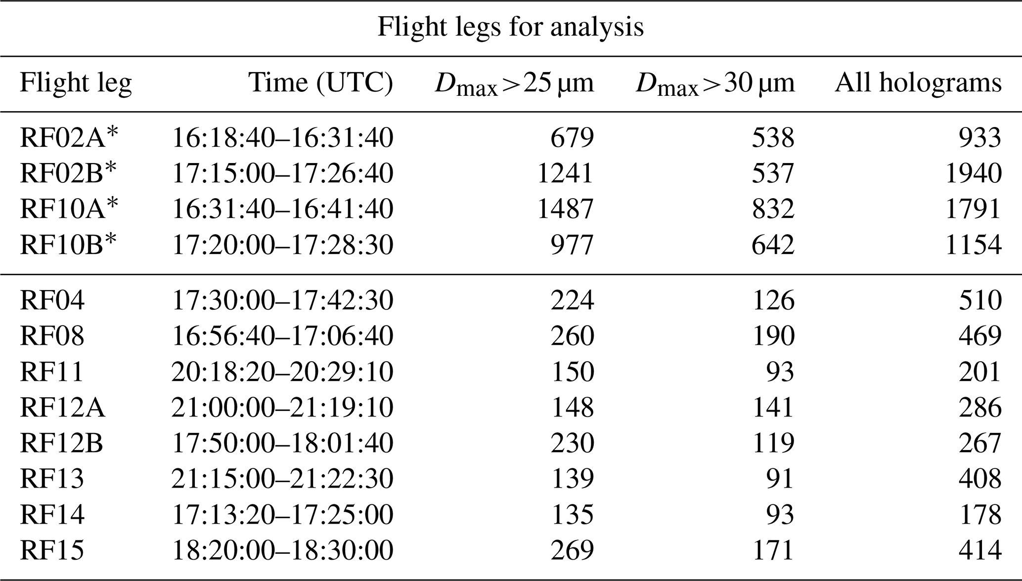
Due to different in-cloud sampling durations amongst the flight legs, 75 % of all available holograms are observed in RF02A, B and RF10A, B (having maximum drop diameter exceeding 25 µm; Table 1). Those flight legs were evaluated in Larsen et al. (2018), who determined radial distribution functions using HOLODEC measurements separately for each flight leg.

2.2 Methodology

Whereas previous studies have quantified droplet clustering of the HOLODEC's respective sample volumes (Glienke et al., 2020; La et al., 2022; Larsen et al., 2018; Larsen and Shaw, 2018;) or the Advanced Max Planck CloudKite holography system's measurement volumes which are similar to the HOLODEC (Thiede et al., 2025), results here evaluate drop clustering on a drop-by-drop basis. In-cloud samples are defined where drop concentrations (N_outer) exceed 100 (per ∼ 3.3 cm³) for consistency with previous clustering analyses of HOLODEC measurements acquired during CSET (La et al., 2022; Larsen et al., 2018; Larsen and Shaw, 2018), which select this threshold to achieve adequate counting statistics when determining drop clustering. Note that Wood et al. (2018) found approximately half of the clouds sampled during CSET have “ultra clean” drop concentrations (∼ 10 cm⁻³), meaning these clouds are not included in the analysis. This study also adapts a similar sample volume as these studies, which is smaller than that reported by the HOLODEC. The reported sample volume dimensions of approximately 1 cm × 1 cm × 13 cm are reduced to 0.6 cm × 0.6 cm × 10 cm, since drop spatial coordinates are more reliable within the inner portion of the sample volume (Larsen et al., 2018). An additional inner sample volume, defined as the guard rail and discussed in the following subsection, is applied so drop sizes are only evaluated within the spatial volume of 0.3 cm × 0.3 cm × 9.7 cm. Previous studies restrict their analysis to drops with D>10 µm as they are assumed to have the best detectability. Drops used here are restricted to sizes of D>12 µm as a lower limit (also for the in-cloud condition), although sensitivity tests using D>10 µm produce results consistent with those shown throughout this study (discussed further in Appendix C).

2.2.1 Introduction to the Radial Distribution Function

Multiple methods exist to quantify droplet clustering, some of which are reviewed in Shaw et al. (2002). The radial distribution function (g(r)) determines the number density of particles as a function of distance from a reference particle, and may be used to quantify particle clustering given three-dimensional particle spatial coordinate data is available. It can be expressed as

$$\begin{array}{}\text{(1)}& g\left(r\right)={\sum }_{i=\mathrm{1}}^N{\displaystyle \frac{{\mathit{\psi }}_i\left(r\right)/N}{\left(N-\mathrm{1}\right)\left(\frac{\mathrm{d}{V}_r}{V}\right)}},\end{array}$$

where ψ(r) is the number of particles surrounding the ith particle within the surrounding spherical shell volume between radii $r-\mathrm{\Delta }r/\mathrm{2}$ and $r+\mathrm{\Delta }r/\mathrm{2}$, V is the measurement volume over the entire hologram, N is the number of drops within the guardrails and dV_r is the measurement volume enclosed within shells having radii $r-\mathrm{\Delta }r/\mathrm{2}$ and $r+\mathrm{\Delta }r/\mathrm{2}$. The equation takes advantage of the notion that a Poisson distribution has evenly distributed particles within a sample volume, which is represented in the denominator of Eq. (1). This means g(r) indicates a greater degree of drop clustering as values increase above 1. An idealized depiction of cloud drops in a hologram is shown in Fig. 1.

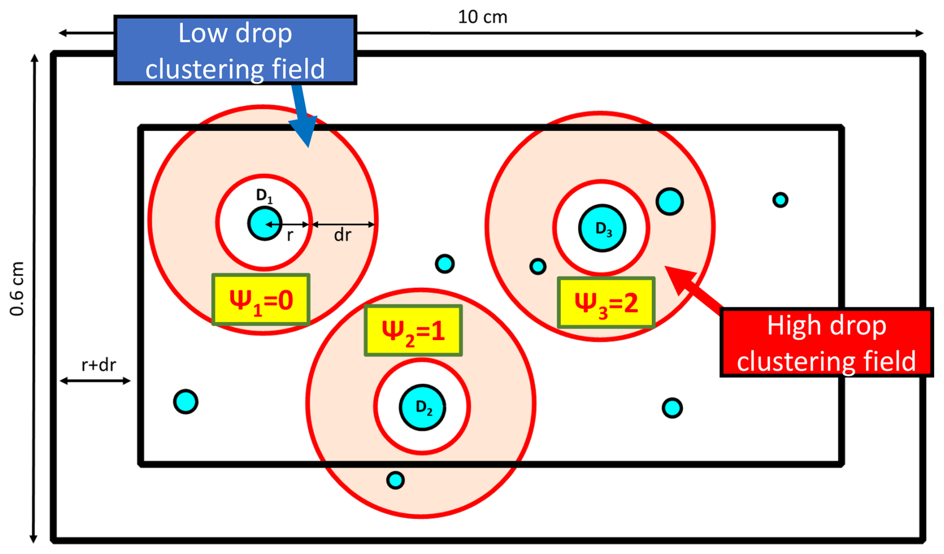
Figure 1 An idealized depiction of drops shown with different numbers of neighboring drops in a hologram. Low (high) drop clustering fields (DCFs) correspond to drops with a significantly low (high) number of neighboring drops (how significance is defined is described in the text). V is the volume of the innermost box and dV is the volume within the light-red shaded spherical annulus volumes of the respective droplets (variables from Eq. 1). Distances are not to scale.

This study employs a guard rail approach which only computes g(r) among the ith particles that are within a certain distance from the measurement volume edges in order to prevent counting biases when computing pairwise correlations. The guard rail distance is the maximum possible shell radius used when computing the radial distribution function ($r+\mathrm{\Delta }r/\mathrm{2}$ in Fig. 1). A detailed overview and visualization of the radial distribution function and guard rail approach can be found in Larsen and Shaw (2018). Two labels within Fig. 1 are denoted “high drop clustering fields” and “low drop clustering fields” (DCFs), which correspond with the drops having the most and fewest neighboring drops within their respective shells. How high and low DCFs are diagnosed using multiple shells sizes is discussed below.

Rather than quantify the clustering of a system (i.e, sample volume) of droplets, this study directly relates drop sizes to their respective DCFs, partly to avoid potential biases associated with the computation of the radial distribution function (illustrative biases are discussed in Part I of the Supplement). The proposed DCF methodology will conceptually mirror DCFs used for determining radial distribution functions, although clustering fields will not be computed at incremental distances away from the droplet centroids. Rather, DCFs will incrementally increase in size while maintaining a constant lower bound.

This “drop-by-drop” method will resemble clustering diagnostics such as pair correlation or the Fishing Test which have previously been applied to single-particle counting instruments (e.g., Baker, 1992; Kostinski and Jameson, 2000; Small and Chuang, 2008), in that clustering is diagnosed relative to individual droplets rather than diagnosing the clustering of drop systems. However, clustering here is not reported as a function of drop pairs using absolute length or time units. Rather, the degree in which drops are clustered or isolated is quantified relative to all the other drops within their respective holograms. The following section will detail the methodology including how droplets are diagnosed as having high/low DCFs.

2.2.2 Particle-by-Particle Methodology

This study aims to directly compare how occurrence frequencies of high and low DCFs differ for different drop sizes. The methodology used to classify high and low DCFs is introduced below, which is derived from the radial distribution function to determine clustering statistics around individual drops. If one were to determine g(r) for an individual drop (g_i), the radial distribution function in Eq. (1) simplifies to

$$\begin{array}{}\text{(2)}& g_{\mathrm{i}}\left(r\right)={\displaystyle \frac{{\mathit{\psi }}_{\mathrm{i}}\left(r\right)}{\left(N-\mathrm{1}\right)\left(\frac{\mathrm{d}{V}_{\mathrm{r}}}{V}\right)}},\end{array}$$

where the summation term is no longer included. Note that total drop concentrations are still included in the denominator to weight the observed number of neighboring drops by the number of drops following a Poisson distribution. However, g_i of individual drops are heavily biased by the total drop concentration term (g_i is greatest at the lowest drop concentrations; Supplement Fig. S2). This is because low, non-zero ψ will significantly exceed the “expected” number produced by the denominator term (a form of counting statistic bias; discussed with further detail later on). Further, one can intuit that greater drop concentrations will increase likelihoods of drops neighboring each other at closer distances relative to lower drop concentrations (given constant sample volumes).

In order to compare DCFs of holograms having notably different drop concentrations, we wish to remove the “expected” (i.e., Poisson) drop count term from consideration. Since we want to determine g_i relative to other drops within their respective holograms, N and V can be removed since they are both constant for each respective hologram. As previously mentioned, DCFs of individual drops are not computed as functions of incremental distance from the drop centroids, but rather as a function of incrementally increasing shell size with a constant lower boundary. This updated individual drop clustering term (C_d) is expressed as

$$\begin{array}{}\text{(3)}& C_{\mathrm{d}}\left(r_{\min }+\mathit{\delta }{r}_n\right)={\displaystyle \frac{\mathit{\psi }(r_{\min }+\mathit{\delta }{r}_n)}{\mathrm{d}{V}_{r_{\min }+\mathit{\delta }{r}_n}}},\end{array}$$

where r_min is a constant lower boundary and δr_n is the width of the spherical annuli (i.e., shell), each starting at r_min whose width increases with increasing n from n=1, …, 7 (top of Fig. 2; discussed below). Note that δr is applied differently than Δr in Eqs. (1) and (2) (illustrated below). It is crucial to maintain constant shell sizes regardless of drop size, rather than vary r_min according to respective drop diameters. Having r_min equal the droplet radius would result in small drops having larger shells compared with large drops given constant δr. A constant r_min of 50 µm is chosen ad hoc, since it is the minimum distance at which two drops having D=50 µm can neighbor each other. Note that the number of drops occurring within r_min and all drop surfaces amounts to ∼ 0.00002 % of all drops, so results are not impacted by this choice of r_min. While this r_min value means that the DCF may not be well-defined for drops with D>50 µm, only ∼ 200 such drops exist in the dataset as defined below, and they are not considered when determining statistical likelihoods of drop sizes for given DCF ranges.

Figure 2 shows an idealized depiction of DCFs within a hologram having multiple shells, where shell sizes increase with a constant lower boundary (r_min) following C_d (Eq. 3). This is seen when comparing δr₁ and δr₂ in Fig. 2. The different shell sizes allow for computation of varying “degrees” of high and low DCFs, where shell sizes are integer multiples of r_min+δr₁ (top row of Fig. 2). The number of shell sizes in our analysis is chosen in order to produce a reasonable resolution for determining spatial correlations between droplets.

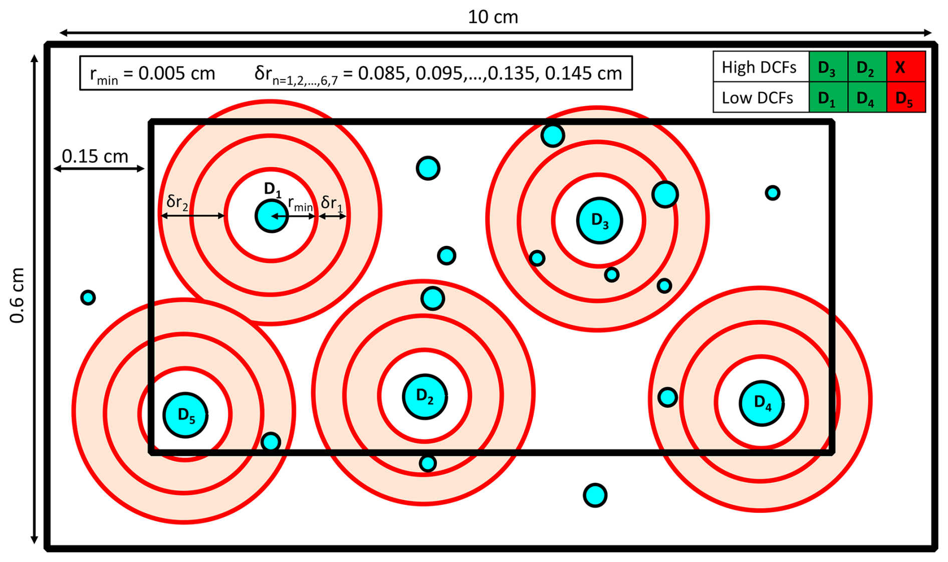
Figure 2 Idealized depiction of high and low drop clustering fields (DCFs) using multiple shells as determined by C_d. DCFs are only shown for select drops (D₁–D₅). The usage of shells follows the proposed methodology and not following RDF (i.e., the lower bound r [r_min] stays constant). The upper left lists the concentric shell size range of radii from 0.09–0.15 cm, with each consecutive shell size increasing in distance from r_min by 0.01 cm. Note that only two shell sizes are shown for simplicity, although the proposed methodology includes seven concentric shell sizes. The upper right panel denotes how high and low DCFs are sorted for their respective maximum to minimum values. Note that D₄ and D₅ have the same values of C_d, and are therefore randomly sorted (discussed in text). The red shading denotes drops not included in the analysis, since the same number of high DCFs and low DCFs must be available from each hologram (discussed in text). Distances are not to scale.

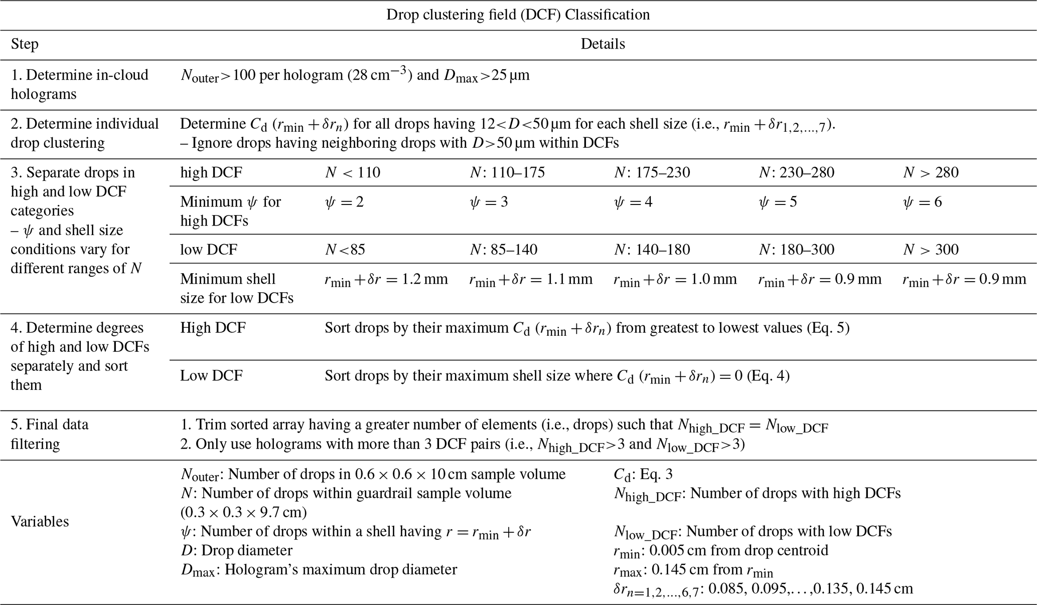
The remainder of this section outlines how individual droplets are diagnosed as being associated with significant clustering (those having high DCFs) or as being significantly isolated from neighboring drops (those having low DCFs), all of which is outlined in Table 2. This diagnosis will consist of two parts. The first part is to diagnose whether drops have a notable degree of high or low clustering. Specifically, in each hologram ∼ $\mathrm{1}/\mathrm{3}$ of the drops will be classified as having high DCFs and ∼ $\mathrm{1}/\mathrm{3}$ of the drops will be classified as having low DCFs (similar to Fig. 1). The second part will be to diagnose the degree of clustering for high DCFs and the degree of isolation for low DCFs. The first step is performed since the degree of clustering and isolation of droplets are computed in different ways, requiring droplets to first be separated into broad DCF categories (high DCFs and low DCFs). This first step is primarily discussed in Appendix A, and is shown as Step 3 in Table 2. The remainder of this section focuses on diagnosing the degree of clustering and isolation of individual drops (Steps 4 and 5 in Table 2). Steps 1 and 2 in Table 2 show that C_d is computed for all droplets, and highlights basic data filtering conditions.

Table 2 All conditions of the Monte Carlo drop clustering field (DCF) classification method which classifies drops as having either high DCFs or low DCFs, as well as determines how degrees of high and low DCFs are computed. Step 3 is discussed in Appendix A. Variable names are provided in the lowest row.

This paragraph focuses on diagnosing degrees of low DCFs, or how isolated drops are from neighboring drops. The degree of isolation is characterized by the drop's largest possible shell size (i.e., r+δr_n) which does not contain any neighboring drops. Drops diagnosed as having “low DCFs” are also sorted by the largest shell size that does not contain any neighboring drops for each hologram. This is depicted in Fig. 2 where D₁ has the lowest DCF, since it is the only drop with no neighboring drops in all available shell sizes. D₄ and D₅ have identical clustering fields, with no drops in the smaller shells. They are then randomly sorted following D₁, due to their identical clustering fields. To further discretize low DCFs, when multiple drops have no neighboring drops within their respective shells of the same size, they are sorted by the number of drops within the maximum shell size of each drop (i.e., $r_{\min }+\mathit{\delta }r=\mathrm{0.15}$ cm). For example, assume there are drops D_a and D_b and both have no neighboring drops within the 0.13 cm shell (i.e., 0.005–0.13 cm from the droplet centroid). D_a and D_b have one drop and three drops within the 0.15 cm shell (i.e., 0.005–0.15 cm from the droplet centroid), respectively. Therefore, D_a is sorted before D_b and has the lower DCF. This means low DCFs are primarily sorted by the largest shell size in which no neighboring drops exist, and when shell sizes are the same, they are sorted by the number of neighboring drops within the maximum shell size. Selecting the maximum shell sizes containing no neighboring drops is comparable to using a Voronoi or nearest neighbor approach for diagnosing isolated droplets. However, a simpler approach is used here since we simply wish to diagnose degrees of drop isolation relative to the holograms they are contained in. The expression for determining low DCFs is shown below.

$$\begin{array}{}\text{(4)}& \mathrm{\text{Low DCF}}=\left\{\begin{array}{l}{\mathrm{rank}}_{\mathrm{holo}}\left({\max }_{n=\mathrm{1},\mathrm{2},\mathrm{\dots },\mathrm{7}}\left(r_{\min }+\mathit{\delta }{r}_n\mathrm{|}{C}_{\mathrm{d}}=\mathrm{0}\right)\right)\\ {\text{if Low DCF}}_{\mathrm{drop},i}\ne {\text{Low DCF}}_{\mathrm{drop},j}\\ {\mathrm{rank}}_{\mathrm{holo}}\left({\min }_{n=\mathrm{1},\mathrm{2},\mathrm{\dots },\mathrm{7}}\left(C_{\mathrm{d}}(r_{\min }+\mathit{\delta }r=\text{0.15\hspace{0.17em}mm})\right)\right)\\ {\text{if Low DCF}}_{\mathrm{drop},i}={\text{Low DCF}}_{\mathrm{drop},j}\end{array}\right.\end{array}$$

where n denotes different shell sizes and the ranking of shell size (r_min+δr_n) is performed relative to each hologram. The top row denotes ranking drops i and j by the maximum shell size containing no drops (C_d=0) amongst all drops within their respective holograms, given both drops do not report the same maximum shell size. If the drops' maximum shell sizes are the same, then they are ranked by $C_{\mathrm{d}}(r_{\min }+\mathit{\delta }r=\mathrm{0.15}$ cm), where drops having lower values are considered to be more isolated. This is shown in the bottom row. Drops reporting similar maximum shell sizes and identical values of C_d(0.15 cm) are randomly sorted.

Utilizing larger shell sizes allows for the ability to diagnose increasingly isolated drops. However, larger shell sizes consequently decrease the guardrail volume, which limits the available sample volume. The upper bound of 0.15 cm is chosen judiciously to diagnose a notable degree of separate between drop pairs while also obtaining a sufficient sample of drops within the bottleneck size range.

Determining high DCFs requires more nuanced consideration, since the shell size and the number of neighboring drops must be considered in unison. Since both terms are considered in C_d, the maximum C_d is selected among all shell sizes when diagnosing high DCFs. This is expressed as

$$\begin{array}{}\text{(5)}& \text{High DCF}={\mathrm{rank}}_{\mathrm{holo}}\left({\max }_{n=\mathrm{1},\mathrm{2},\mathrm{\dots },\mathrm{7}}\left(C_{\mathrm{d}}\left(r_{\min }+\mathit{\delta }{r}_n\right)\right)\right)\end{array}$$

where n denotes different shell sizes and the ranking of the maximum C_d (amongst all available shell sizes) is performed relative to each hologram. If two drops have identical maximum C_d, they are randomly sorted. Supplement Fig. S3 shows how different C_d rank amongst each other for varying ψ(r_min+δr) and shell sizes.

When performing drop-by-drop comparisons, the same number of drops possessing high and low DCFs are selected from each hologram to control for environmental conditions (Step 5 of Table 2). Namely, by selecting the same number of drops possessing high and low DCFs from each hologram, we control for environmental factors and bulk properties (e.g., RH, N, etc.) since the same number of high and low DCFs will be associated with any given environmental/microphysical variable. To achieve this, the DCF category with the greater number of drops is reduced to have the same number of drops as the lower category. Drops are removed at random to produce an equal number of drops between the DCF categories. Sampling with replacement of the smaller drop category in order to retain a greater number of droplets is also possible. However, the current methodology results in approximately one third of drops having high DCFs, low DCFs and DCFs within these two ranges (shown in Appendix A). And since results will primarily focus on the highest and lowest DCFs (Sect. 3), there is no need for sampling with replacement. The requirement of at least 4 high and low DCFs within each hologram (Step 5 in Table 2) will be discussed in relation to the Monte Carlo-DCF methodology below, and results in ∼ 5 % of available holograms being discarded.

3 Statistical testing for drop clustering

Up to this point, a methodology has been introduced to classify high DCFs (i.e., drops having a high number of neighboring drops) and low DCFs (i.e., drops notably isolated from surrounding drops), which is outlined in Steps 1–5 in Table 2. DCFs are categorized relative to the drop concentrations of their respective holograms, meaning high DCFs will likely contain fewer drops in holograms with low drop concentrations compared with high DCFs in holograms having high drop concentrations. This section introduces two methodologies to evaluate the relationships of drop sizes to their respective DCFs – both of which rely on some form of Monte Carlo analysis. Section 3.1 is a description of how the statistical likelihood of DCFs are determined in relation to their respective drop sizes. Section 3.2 introduces a methodology to discern which environmental/microphysical parameters are most notably related to DCF signals of interest.

3.1 Methodology No. 1: Monte Carlo-DCF methodology

To determine how high and low DCFs relate to drop sizes (i.e., whether clustering tends to be greater around larger and/or smaller drops), a statistical methodology using Monte Carlo simulations is applied to each hologram. This will be referred to as the Monte Carlo-DCF methodology. Namely, for each simulation the drop sizes within the inner guardrail sample volume are randomly shuffled amongst the drops within this sample volume. Only the drop sizes are randomly sorted while the original drop spatial coordinates remain unchanged – meaning the DCFs will be identical for each hologram. For example, the drop sizes in Fig. 2 (D₁, D₂, …, D₅) will be randomly assigned to the drops within the hologram. This is to provide a counterfactual where no relationship between DCFs and drop sizes exists. Since DCFs remain unchanged, the same number of drops meeting the high/low DCF classifications are selected from each hologram. The observed drop size–DCFs relationships are then compared to the simulated drop size–DCFs relationships. One thousand Monte Carlo simulations are run for all holograms used in this study. Findings directly applying this methodology are provided in Sect. 4.1, where further detail is provided.

3.2 Methodology No. 2: Monte Carlo-Hologram Comparison methodology

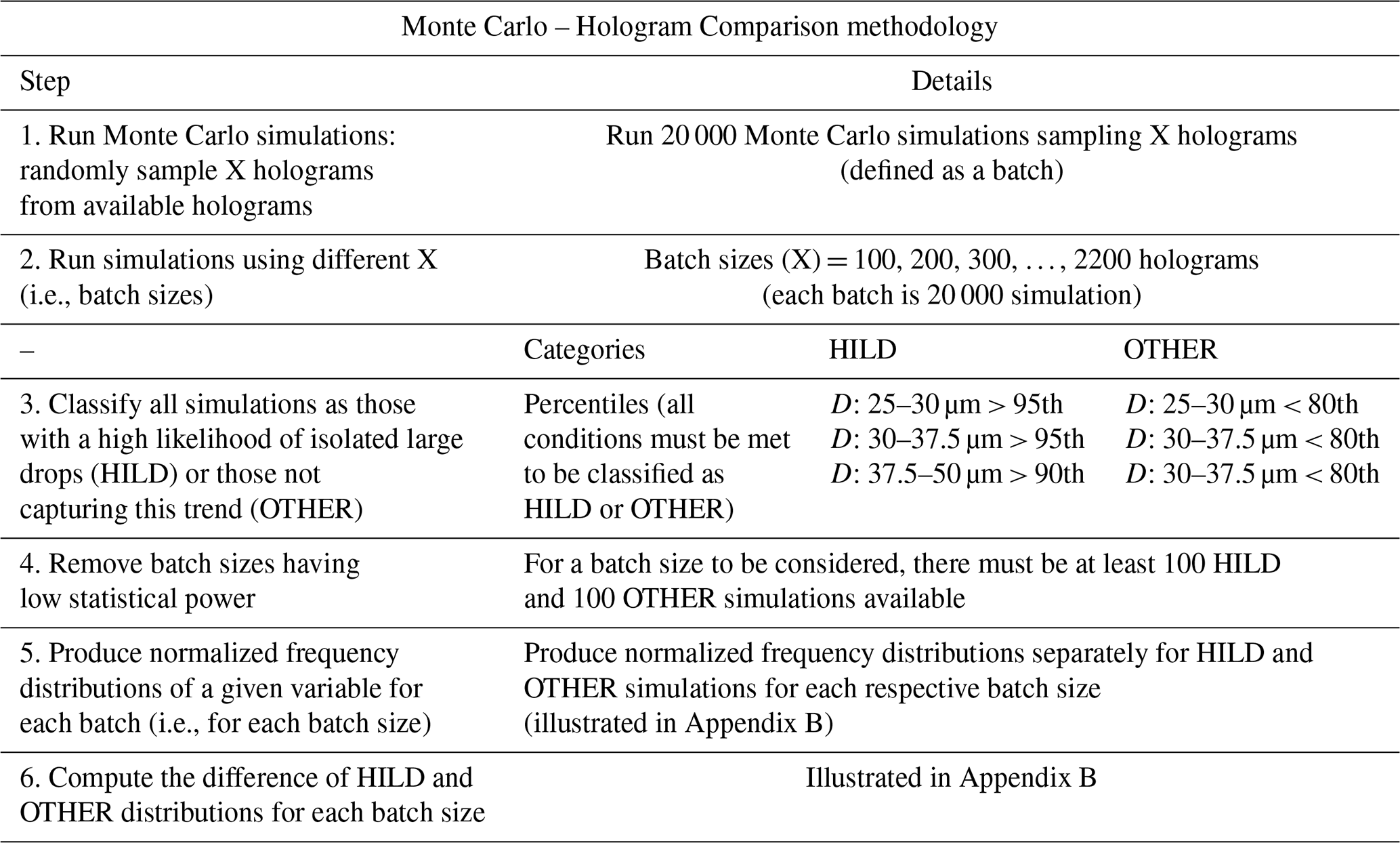
The drop clustering method in Table 2 will allow us to examine the relationship between drop size and DCF as a function of some environmental variable (e.g., whether the holograms come from subsaturated or supersaturated regions; shown in Sect. 4.1). However, this requires the manual selection of holograms when exploring DCF–drop size relationships and may result in Type-I errors (i.e., falsely rejecting the null hypothesis). A second methodology is proposed here to discern which variables are associated with notable DCFs–drop sizes relationships, without the manual selection of holograms. This is called the Monte Carlo-Hologram Comparison methodology, and is used in Sect. 4.2. The methodology is outlined in Table 3.

First, a specified number of holograms (X) are randomly selected from all available holograms (Step 1 in Table 3). This is defined as one simulation, and 20 000 simulations are run for a given number of randomly selected holograms. This is repeated for different X (i.e., different numbers of randomly selected holograms; specified in Step 2 of Table 3). DCF–drop size relationships are then determined for each simulation using the Monte Carlo-DCF methodology from Sect. 3.1. Simulations are separated into one of two categories: those where an “isolated large drop trend” (i.e., drops within bottleneck range are most likely to be isolated from other drops) is observed and those where it is not. In other words, the former category contains simulations having high likelihoods of isolated large drops (HILD) and the latter category contains simulations not possessing this signal (OTHER) (Step 3 of Table 3).

The associated environmental/bulk microphysical variables are also separately obtained from the HILD and OTHER simulations, and their occurrence frequencies are then compared with each other to determine the likelihoods that these variables are associated with this isolated large drop trend. This is done by producing normalized frequency distributions of the given variable for each of the two categories, and then computing the differences between the distributions over each size bin. A step-by-step description of the methodology is provided in Appendix B.

Table 3 Components of the Monte Carlo-Hologram methodology. Details/further clarification of the methodology are described in the text and in Appendix B.

Only holograms from flight legs RF02A, B and RF10A, B are included in the Monte Carlo-Hologram Comparison methodology, because the random selection of holograms will consequently draw from these flight legs having significantly more holograms. This is also done in order to perform separate flight leg comparisons, which will become evident in Sect. 4.2. Note that each individual simulation above may include holograms from multiple flight legs. A more detailed description of the Monte Carlo-Hologram Comparison methodology is provided in Sect. 4.2 and Appendix B.

4 Results

4.1 Initial DCF – drop size relationships

Figure 3 shows results from the Monte Carlo-DCF methodology for different sampling conditions overlying the respective panels (bold text). The overlying elongated panels (A–D) show percentiles of actual drop sizes having either high or low DCFs (red and blue markers, respectively) in relation to those of the Monte Carlo simulations. The percentiles are derived from drop size histograms shown in Fig. 3A1–D1, where the thick red and blue lines are histograms of the observed drops having high and low DCFs, respectively. The number of drop size counts in each bin (lightly shaded dotted lines) is related to those from the histograms of the Monte Carlo simulations, which are shown as thin red and blue lines (although they are often overlapped by the actual DCF distributions). The next paragraph will zoom in on one of these histograms to clarify the analysis, which ultimately determines whether a given DCF category/degree of high or low DCF will be more or less likely associated with drops of a certain size range.

We first focus on the top left panels: Fig. 3A shows percentile results for drop sizes categorized as having high and low DCFs amongst all holograms used in this study. A few “statistically significant” drop size ranges can be found, i.e., DCFs either below or exceeding the 5th and 95th percentiles, respectively (represented by the diamonds and stars). This includes a statistically significant drop size range from 30–37.5 µm. To better illustrate the comparison between the actual and Monte Carlo distributions, the 30–37.5 µm drop size bin from Fig. A1 is magnified and displayed in the middle of the figure. The drop size distributions from the Monte Carlo simulations can now be seen as the thin red and blue lines (although giving a partial appearance of purple lines due to their overlap), corresponding to the high and low DCFs, respectively. The actual number of drops having low DCFs (thick blue line) in this bin exceeds the number of drops having low DCFs for most of the Monte Carlo simulations (thin blue lines), specifically exceeding over 95 % of them. We define cases where the actual number of counts in a drop size bin is greater (less) than those for 95 % (5 %) of the simulations as being statistically significant. Therefore, drops having low DCFs are significantly likely to possess D ranging from 30–37.5 µm.

Section 2 discussed how drops with varying degrees of high and low DCFs are sorted (top right corner of Fig. 2). And since the same number of high and low DCFs are selected from each hologram, percentiles of DCF “degrees” (Step 4 in Table 2) can be obtained for direct comparison with each other. To focus on drops with increasingly greater degrees of high DCFs (i.e., larger maximum values of C_d) and low DCFs (drops increasingly isolated from neighboring drops), Fig. 4B shows results restricted to drops with DCFs above the 50th percentile, and Fig. 4D shows results restricted to the upper tercile (DCFs > 67th percentile). For example, if results were shown only for the hologram in Fig. 2, the results in Fig. 4A, A1 would correspond with analyzing drops D₁₋₄ (green shaded drops in top right panel), and results in Fig. 4B, B1 would correspond with only analyzing drops D_1,3.

Results from panel (A) are considered our exploratory analysis by looking at all available data. However, all of the drop sizes exceeding 25 µm are associated with relatively high percentiles of low DCFs, including a statistically significant drop size range from 30–37.5 µm. Excluding the lowest drop size bin, a trend of increasing percentiles with increasing drop size is observed for low DCFs (blue markers). Because of this, we hypothesize the lowest DCFs should be associated with large drops (D > 25 µm), likely because dry air preferentially evaporates small droplets due to their greater surface area to volume ratio relative to larger drops. We test this hypothesis by looking at drops with increasingly lower DCFs (Panels B and D). Consistent with the hypothesis, DCF percentiles increase for large drops moving from panels (A) to (B) and finally (D) – as seen by the increasing number of blue diamonds and stars. Namely, percentiles of large drops having low DCFs increase with increasingly lower DCFs. In other words, drops within the bottleneck size range are most likely to be significantly isolated from surrounding drops. This finding is further suggested by results with “moderate” DCF values below the 50th percentiles (Fig. 3C), which show no significant differences of low DCFs between the observations and Monte Carlo simulations for large drops (i.e., no increased likelihoods of large drops having low DCFs, seen by blue points for D>25 µm).

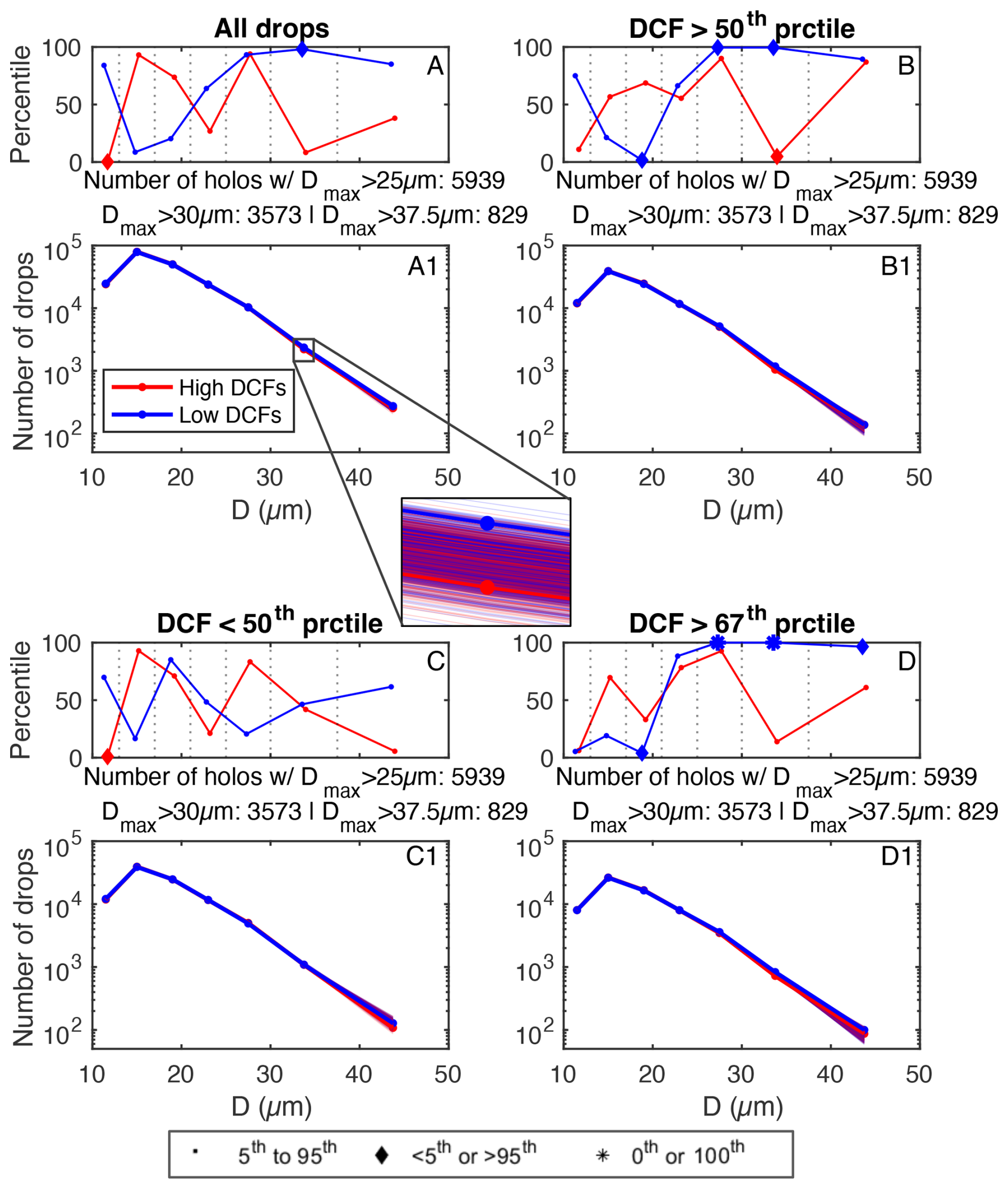
Figure 3 (A) Percentiles of drop size occurrence frequencies in relation to simulated occurrence frequencies for all drops from all holograms used in the analysis – described in further detail in the text. Red markers correspond to drops with high drop clustering fields (DCFs) and blue markers correspond to drops with low DCFs. Similar results are shown but restricted to greater degrees of high and low DCFs, greater than the respective holograms' median values (i.e., degrees of high and low DCFs > 50th percentiles; (B) below the median values (C) and in the upper tercile (D). Markers are denoted by multiple marker shapes, where points correspond to percentiles ranging from the 5th–95th, diamonds correspond to percentiles below (exceeding) the 5th (95th) percentiles, and stars correspond to percentiles below (exceeding) the lowest (highest) simulated occurrence frequencies (bottom legend). The number of drops in each DCF category is shown underlying the respective percentile plots (thick lines; A1–D1), which also include thin red and blue lines denoting results from the Monte Carlo simulations. Note that Monte Carlo simulation frequencies are all nearly overlapped by those of the observed DCF categories. Results are restricted to holograms having D_max>25. The number of holograms having different D_max are shown immediately below the respective percentile panels.

Results in Fig. 3 were taken from all available holograms, meaning drops were selected from all holograms regardless of environmental or other external conditions. This is why the number of holograms remains unchanged for each pair of panels. Figure 4A, C shows results separating holograms by subsaturated and supersaturated conditions (RH < 99.5 % and RH > 100.5 %, respectively) and Fig. 4B, D shows results separated by relatively low and high drop concentrations. Holograms are selected from collocated 1 Hz RH measurements having relatively coarse spatial resolutions (∼ 100 m; previously described in Sect. 2.1). Results here are limited to DCF percentiles in the upper tercile (similar to Fig. 3D). Findings show that the increased likelihoods of large drops being isolated from neighboring drops are observed for subsaturated conditions and relatively low drop concentrations (occurrence frequencies of D > 25 µm exceed the 95th percentile for low DCFs in Fig. 4A, B). Both of these conditions are expected with entrainment, as environmental dry air engulfed into the cloud commonly decreases drop concentrations (via inhomogeneous mixing). However, most samples from CSET have these relatively low drop concentrations, which are expected in marine environments (including the CSET measurements: Wood et al., 2018; Bretherton et al., 2019). The vast majority of high drop concentrations come from RF02B and RF10A (both with median N exceeding 115 cm⁻³, not shown), which will be discussed further below.

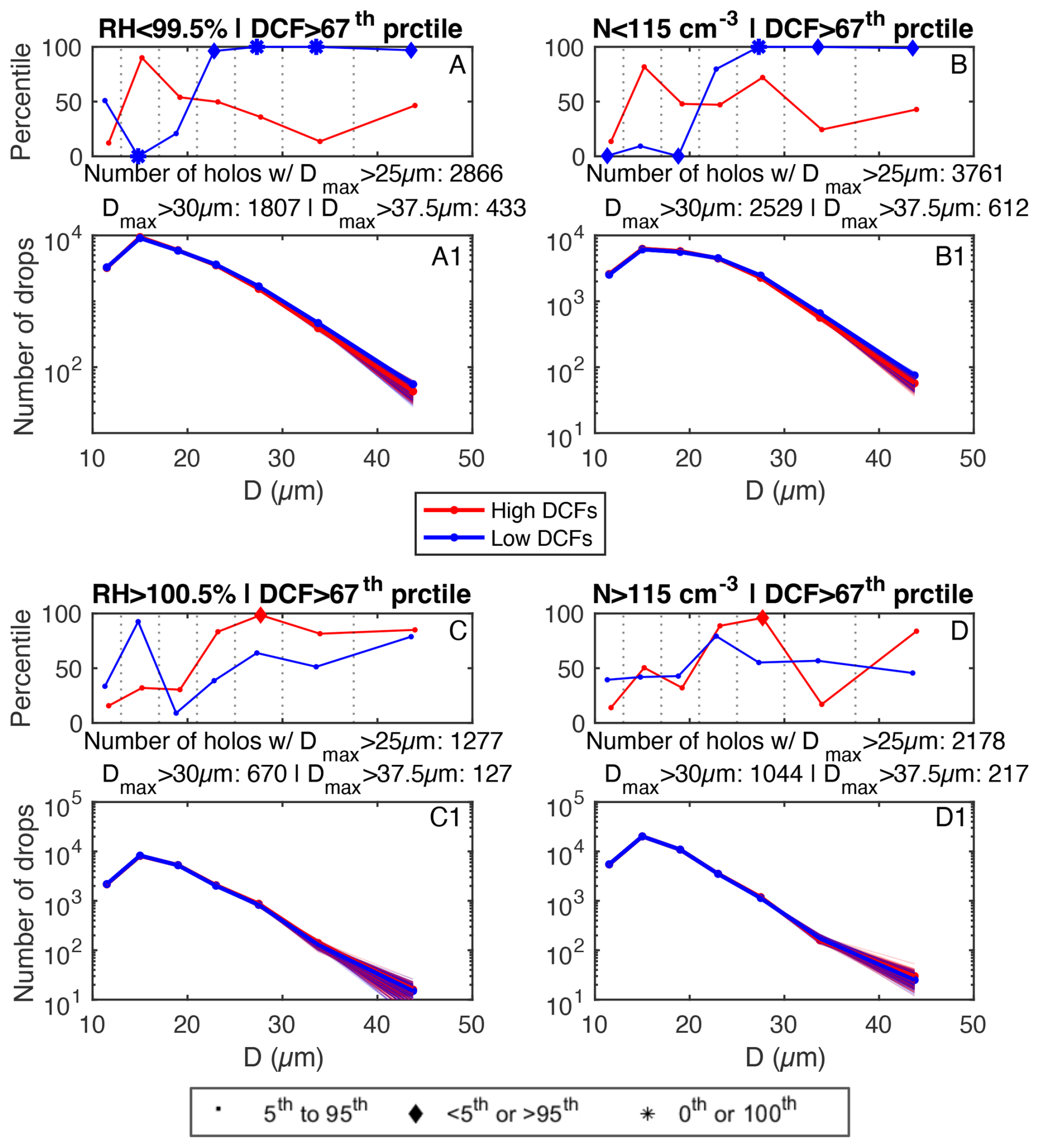
Figure 4 Similar to Fig. 3D, D1, except holograms are separated into subsaturated conditions (RH < 99.5 %; (A) low drop concentrations (N<115 cm⁻³; (B) supersaturated conditions (RH > 100.5 %; (C) and high drop concentrations (N > 115 cm⁻³ (D).

Due to the limited number of flight legs available for analysis, an analysis of DCFs for separate flight legs is warranted. This is to determine whether macro-scale features not evident from localized in situ measurements may correspond to this isolated large drop trend. Two examples are a dependence on cloud regime or background aerosol conditions. Aerosol properties cannot be determined locally due to major biases associated with in-cloud measurements from instrumentation such as aerosol spectrometers and cloud condensation nuclei counters (e.g., Hudson and Frisbie, 1991). As previously mentioned, 75 % of available holograms having D_max > 25 µm are from flight legs RF02A, B and RF10A, B (Table 1). Figure 5 focuses on these flight legs – showing percentile data similar to Figs. 3, 4 but for each of these flight legs separately.

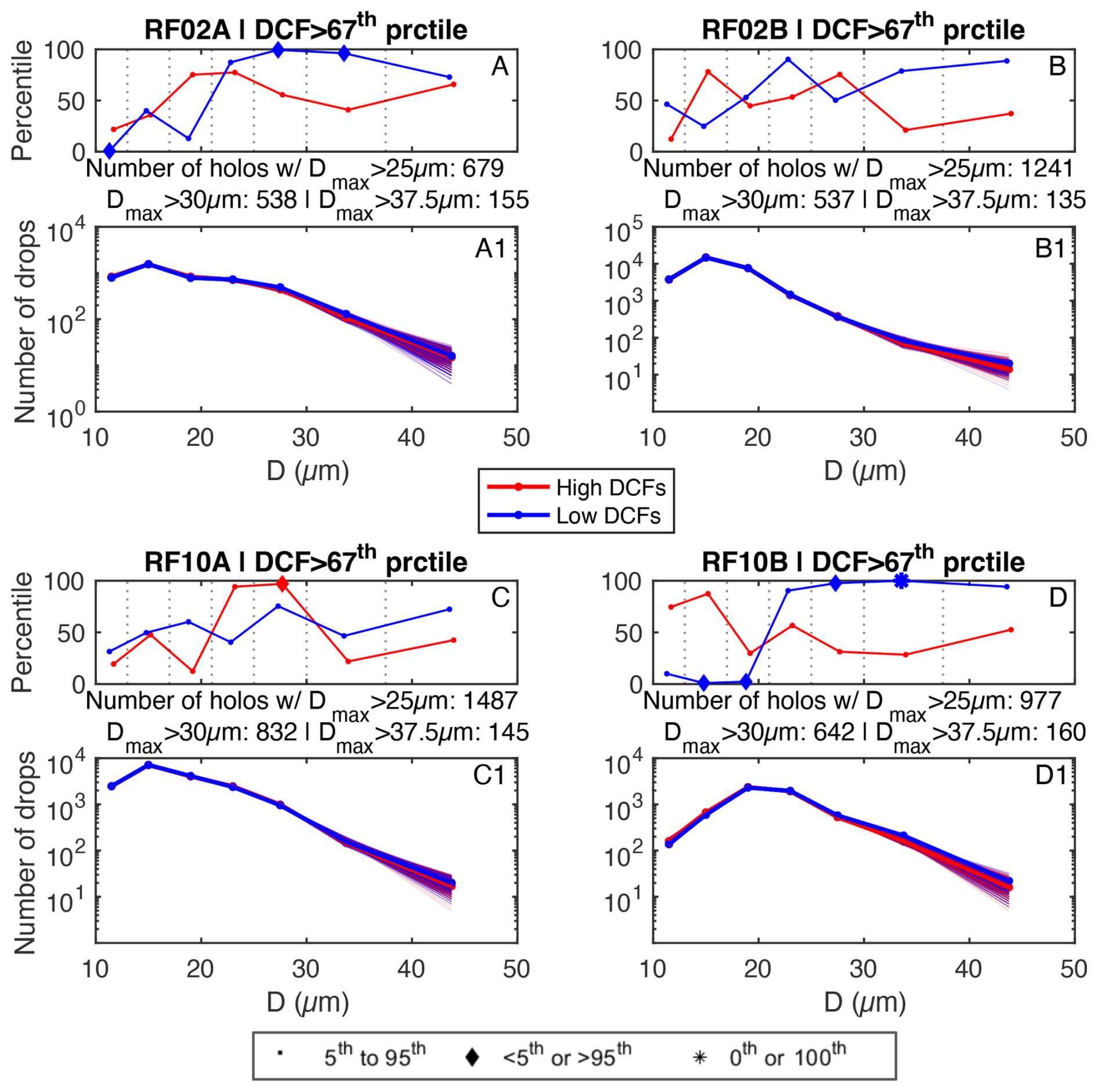
Figure 5 Similar to Figs. 3, 4 but shown for flight legs RF02A, B and RF10A, B (A&A1, B&B1, C&C1, D&D1, respectively).

Amongst the four flight legs, the isolated large drop trend is only observed for RF02A and RF10B (Fig. 5A, D). This will be motivation to focus attention on DCF trends for these two flight legs in the following section.

4.2 Monte Carlo simulations – Hologram comparisons

Manually selecting holograms (e.g., separating results by holograms in sub-/supersaturated environments) may not be the best way to determine which variables are associated with the isolated large drop trend, since this approach may result in a particularly egregious case of p-hacking (i.e., testing combinations of holograms until “satisfactory” results are obtained; possibly resulting in Type-I errors). To mitigate this, we employ a different Monte Carlo analysis where each simulation randomly selects a number of holograms and determines the DCF–drop size likelihoods as in Figs. 3–5.

Multiple simulations are run to determine what conditions are associated with holograms displaying the “isolated large drop” trend, which is detailed in Table 3. Sets of 20 000 simulations are run (i.e., batches), where each simulation set consists of randomly selecting a set number of holograms (i.e., batch size) from all available holograms. A variety of batch sizes ranging from 100 to 2200 are used since it is unclear which/how many holograms are the main contributors to the isolated large drop trend. Simulations are separated into two categories: (1) those having a High likelihood of Isolated Large Drops (HILD) and (2) those not exhibiting the isolated large drop trend (OTHER). The drop bins used to determine likelihoods are kept consistent with those in Figs. 3–5, and the conditions for each category are shown in Step 3 of Table 3. Note the less stringent threshold applied to the 37.5–50 µm diameter bin (exceeding the 90th percentile rather the 95th as for the 25–30 and 30–37.5 µm bins) approximately doubles the available number of simulations included in the HILD category. This “lax” condition we argue is applicable due to the relatively low number of drops in this largest D bin. In order to improve the empirical power of the batches (i.e., number of simulations rejecting the null hypothesis divided by the total number of simulations), batches of a given size must have at least 100 HILD simulations and 100 OTHER simulations to be included in the analysis (Step 4 in Table 3). Samples of a given variable are then separately obtained from the HILD and OTHER simulations, and are then converted into normalized frequency distributions for each batch size. The difference of the HILD and OTHER distributions is then computed over all respective bins. Distributions are normalized since the Monte Carlo sampling captures different numbers of HILD and OTHER simulations for each batch size (Seen in Fig. B1A in Appendix B). A more detailed description and illustration of the methodology is provided in Appendix B.

Figure 6 shows the difference in the normalized frequency distributions (i.e., HILD – OTHER) of different variables as box plots from all available batch sizes. Results are separately shown for the analysis applied to all holograms having D_max > 25 µm (red box plots) and for all holograms having D_max > 30 µm (blue box plots) to test for consistency. There are 17 batches for D_max > 25 µm and 10 batches for D_max > 30 µm in the analysis having sufficient empirical power (Step 4 in Table 3). The gray lines are histograms showing the number of holograms with D_max > 25 µm, which correspond to the right ordinates. The HILD – OTHER differences show how given parameters are related to the isolated large drop trend. For example, positive values of HILD – OTHER show that a greater number of holograms possessing values of a given parameter are associated with the isolated large drop trend, and vice versa. We reminder the reader that results here are only shown for flight legs RF02A, B and RF10A, B. Supplement Fig. S4 is similar to Fig. 6 except all twelve flight legs are used, and all major trends discussed below are still observed.

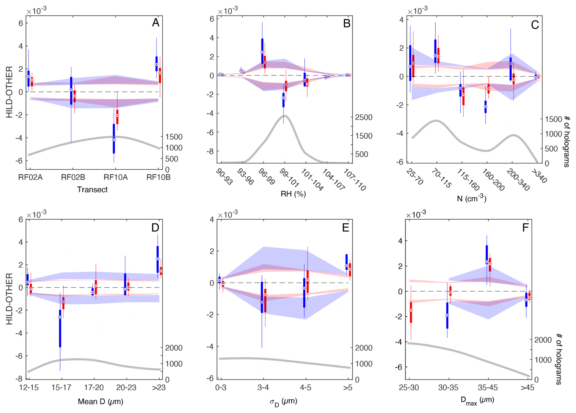
Figure 6 Differences in the normalized frequency distributions of the HILD and OTHER batches for number of flight leg samples (A), RH (B), N (C), number weighted mean diameter (mean D) (D), the standard deviation of drop diameter (σ_D) (E) and D_max (F). Results are displayed as box plots containing differences for all batch sizes (described in the text and Appendix B). Red and blue box plots display batch differences selecting from holograms with D_max>25 and D_max>30 µm, respectively. The dashed line is shown where the difference equals 0. Colored shading overlying and underlying the dashed line corresponds to upper and lower bound confidence intervals, respectively. Confidence intervals are displayed as the maximum and minimum 80th percentiles of statistical significance taken from the 25th, 50th and 75th percentile differences for each respective bin (i.e., corresponding to simulation sets of the bottom, middle dot and top of the box plots, respectively). A description of how significance is determined as well as justification for selecting an 80th percentile level of significance is provided in Appendix B. The grey lines show histograms of the respective variables from the dataset corresponding to the right ordinates. Histograms have the same bin sizes as the overlying box plots and have a cubic interpolation applied to them.

The HILD – OTHER differences for number of samples within flight legs, RH and N (Fig. 6A, B, C) are consistent with trends from Figs. 4, 5. The HILD simulations have a greater number of holograms taken from flight legs RF02A and RF10B (Fig. 6A), consistent with flight legs capturing the isolated large drop trend in Fig. 5. The HILD simulations also have a greater number of subsaturated samples as well as a greater number of relatively low drop concentrations (N<115 cm⁻³), consistent with trends in Fig. 4. Trends are broadly consistent between those selecting holograms from different D_max datasets (red and blue box plots).

The HILD – OTHER differences are shown for the number weighted mean diameter (mean D) in Fig. 6D. The HILD simulations are primarily associated with the largest mean D (> 23 µm), which is consistent with our theory of smaller droplets preferentially evaporating due to their greater surface area to volume ratio. To explore whether there is any evidence of entrainment-mixing drop size distribution broadening, HILD – OTHER differences are similarly shown for the standard deviation of drop diameters (σ_D) (Fig. 6E) and for D_max (Fig. 6F). Positive differences are associated with the largest σ_D (σ_D > 5 µm), consistent with entrainment-mixing drop size distribution broadening. Finally, positive differences are observed for relatively large D_max, ranging from 35–45 µm. However, holograms with D_max exceeding 45 µm are not associated with the isolated drop trend. This either suggests entrainment-mixing broadening is only capable of producing drop diameters within this approximate range, or the methodology fails to adequately capture a signal from holograms containing D_max exceeding 45 µm due to the relatively small sample size of such holograms (92). Using all available flight legs only increases the available number of holograms by 40. The relation of these trends to the presence of drizzle will be revisited later on.

Findings so far have displayed results for all flight legs in combination. However, the isolated large drop trend may be a consequence of macro-scale features associated with given flight legs (e.g., aerosol fields), and trends in Fig. 6 may simply correspond to the respective flight legs while other trends are epiphenomenal. To explore this possibility, the remaining results will look at how the isolated large drop trend is associated with different flight legs. Figure 7 shows HILD – OTHER differences similar to Fig. 6 but for separate flight legs (rows). The columns show HILD – OTHER for different variables. As in Fig. 6, samples are restricted to RF02A, B and RF10A, B due to the notably greater number of available holograms from these flight legs. This is because it is difficult to determine which flight legs have the most “notable” isolated large drop trend for flight legs with varying numbers of in-cloud samples, since more holograms will be pulled from flight legs with more measurements. Histograms of the variables' occurrence frequencies in Fig. 7 are shown for each flight leg separately in Supplement Fig. S5.

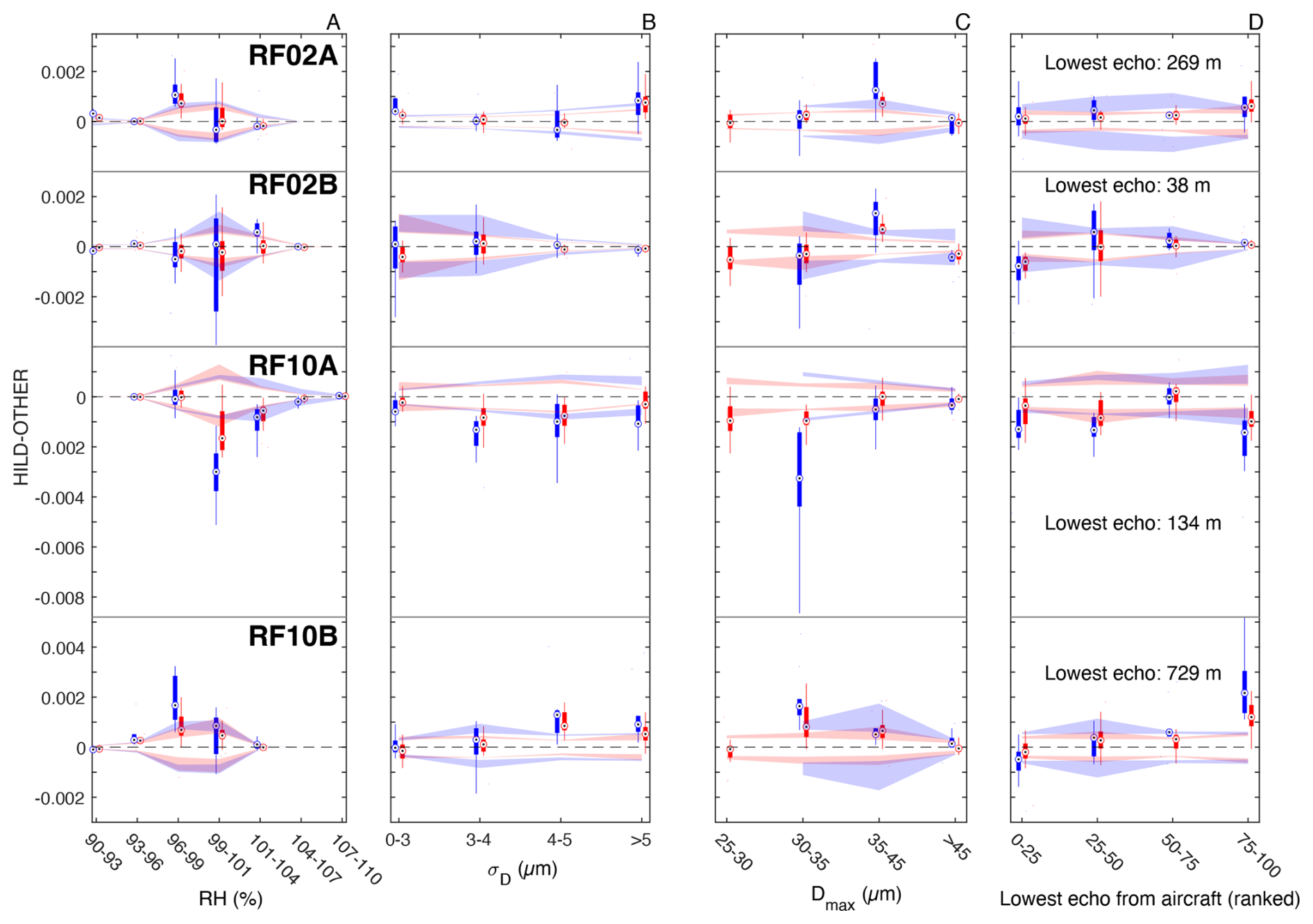
Figure 7 Similar to Fig. 6 except shown for separate flight legs (rows). The panels show HILD – OTHER differences for RH (A), σ_D (B), D_max (C), and ranked distance from the aircraft to the lowest return echo (described in the text; D). Distances in (D) are ranked from 0 (highest altitude) to 100 (lowest altitude) for each respective flight.

Focusing first on results for RH (Fig. 7A), positive HILD – OTHER are only observed in the bin of 96 %–99 % for RF02A and RF10B, the two flight legs associated with the isolated large drop trend (Fig. 5). Results shown for σ_D (Fig. 7B) similarly show positive HILD – OTHER for the largest σ_D values for these two flight legs. This is similarly restricted to the two flight legs associated with the isolated large drop trend. This suggests that the isolated large drop trend is related to the reported microphysical properties and not macro-scale features of the flight legs. Results for D_max (Fig. 7C) also capture positive HILD – OTHER for D_max from 35–45 µm for these two flight legs, and it is also captured for RF02B (2nd row). The trend is relatively weak in RF10B, especially since positive HILD – OTHER are also seen for D_max from 30–35 µm (4th row). This weak trend may be due to the fact that drizzle is weakening the signal, since a clear precipitation signal from this flight leg is visible in radar imagery (not shown). This is possibly suggested by the differences in boxplots for the D_max datasets > 25 and > 30 µm. The positive HILD – OTHER signal is weaker when selecting among the D_max > 30 µm dataset, which could be selecting from a greater number of samples influenced by descending drizzle drops/collision-coalescence compared to the D_max > 25 µm dataset.

To test this assumption, results in Fig. 7D are shown for the lowest radar detection of cloud, and the values are ranked from 0 (highest altitude) to 100 (lowest altitude) for each respective flight. We assume regions of the cloud with the lowest reaching condensate are likely associated with those producing the largest drops, since they will take longer to evaporate during descent. We also assume this variable has a greater “memory” for precipitation-initiation detection, since relatively larger drops are often either swept in/out or fall in/out of any given hologram. The lowest altitudes where condensate is detected relative to the aircraft is shown in meters for each respective flight, with the two lowest values from the flight legs associated with the isolated large drop trend (top and bottom rows). Values are ranked since ranges of the lowest condensate vary considerably among the flight legs (Fig. S5D), and ranking also produces uniform distributions so that 25 % of samples are within each of the four bins. Note that positive HILD – OTHER are observed at the largest ranked values for the two flight legs associated with the isolated large drop trend (7D; top and bottom row). The largest difference is observed for RF10B which far exceeds the uncertainty bounds, the flight leg with condensate reaching the lowest altitudes as well as the clearest precipitation signal amongst the four flight legs from visible inspection of radar reflectivity (not shown).

5 Implications of findings

The cumulative results from Figs. 6, 7 suggest that the isolated large drop trend is related to entrainment-mixing, and presents evidence for entrainment-mixing drop size distribution broadening and its relevance for precipitation initiation. Alternative precipitation initiation mechanisms consistent with this isolated large drop paradigm include “Ostwalt ripening” (e.g., Çelik and Marwitz, 1999; Wood et al., 2002) and the turbulent sorting of droplets enhancing supersaturation within regions of high vorticity (Shaw et al., 1998). However, neither mechanism accounts for the isolated large drop trend occurring primarily in subsaturated conditions. Thus, results appear to be most consistent with entrainment-mixing drop size broadening.

At first consideration, the isolated large drop trend could solely result from the removal of small drops via preferential evaporation due to their greater surface area to volume ratio relative to larger drops (where drops are impacted by micro-scale temperature/vapor fields). However, holograms experiencing this trend are also associated with broader drop size distributions (Fig. 6E) and larger drops than holograms not exhibiting this trend (Fig. 6F). Further, this trend is associated with portions of the cloud where precipitation/condensate reaches the lowest altitudes from the respective cloud (which may invalidate the presence of Ostwald ripening assuming the parcels' locations vary considerably over timescales on the order of hours; Fig. 7D). The totality of findings here is therefore consistent with entrainment-mixing drop size broadening as a relevant precipitation-initiation mechanism (e.g., Lasher-Trapp et al., 2005; Hoffmann et al., 2019). It should be acknowledged that the bottleneck size range is loosely defined among previous studies, often defining the lower bound diameter ranging between 20–40 µm and the upper bound diameter ranging from 40–80 µm (Glienke et al., 2017; Grabowski and Wang, 2013; La et al., 2022; Pruppacher and Klett, 1996; Taraniuk et al., 2008). Results here are restricted primarily to the lower bound, due to the low sample size of drops at the larger end of the bottleneck range. Because of this, results may primarily capture a diffusional-growth process only relevant to relatively smaller bottleneck droplets – and caution should be taken before disregarding alternative precipitation-initiation mechanisms not associated with the isolated large drop trend. A sensitivity test slightly increasing the guardrail dimensions to be 0.4 cm × 0.4 cm × 9.8 cm (and accordingly the outer sample volume increased to 0.7 cm × 0.7 × 10.1 cm) was performed with the hope of sampling more/larger bottleneck drops. Unfortunately, due to the commonly observed quasi-exponential decrease in drop concentrations with increasing drop size beyond D ∼ 20 µm (shown for drops having high and low DCFs in Fig. 3A1), an “adequate” number of large bottleneck drops was still not captured. Additional sensitivity tests/suspected uncertainties are discussed in Appendix C.

6 Concluding remarks

The purpose of this study is to present a new analytic paradigm for exploring possible correlations between drop clustering and drop size, which are theorized to be associated with varying microphysical processes such as precipitation initiation. A novel method is introduced here to evaluate drop clustering on a drop-by-drop basis, where the degree of clustering and isolation of drops is quantified relative to those in their respective sample volumes. This is in contrast to previous studies reporting clustering in terms of absolute length or time scales, as well as previous holography studies primarily diagnosing drop clustering of given “drop systems” (i.e., sample volumes). Measurements are acquired using the HOLODEC probe, which is ideal for evaluating drop clustering due to the constant 3D sample volume size for each hologram. For each hologram, all droplets are first labeled as either (1) having a significantly high number of neighboring drops, (2) being significantly isolated from other drops or (3) meeting neither condition. Then Monte Carlo simulations are run, randomizing the drop sizes in each respective hologram while preserving the drop locations. This allows us to determine likelihoods that drops having a given size are either associated with a significant number of neighboring drops or as being significantly isolated from other drops. Results here show drops having sizes within the bottleneck size range (D ∼ 25–50 µm) are commonly the most isolated drops within their respective holograms.

Additional analysis is performed to determine under which conditions holograms are associated with this “isolated large drop” trend. Holograms in subsaturated conditions and having low drop concentrations are associated with this trend, both of which suggest the isolated large drop trend is directly related to the presence of entrainment. These standalone findings could simply be the result of smaller drops preferentially evaporating due to their greater surface area to volume ratio relative to larger drops. However, holograms associated with the isolated large drop trend also have broader drop size distributions, larger maximum drop sizes and tend to overlie regions where cloud condensate/precipitation reaches the lowest altitudes. The totality of these findings suggests entrainment-mixing drop size broadening is a relevant precipitation initiation process, which has been suggested in previous modeling studies highlighting the ability of entrainment-mixing to produce “precipitation embryos” (e.g., Hoffmann et al., 2019; Lasher-Trapp et al., 2005). Notably, the isolated large drop trend is localized to a few flight legs, which may suggest its relevance is restricted to condition(s) beyond those analyzed here (e.g., background aerosol properties).

Previous studies using similar holography measurements have found no correlation between the occurrence of drops in the bottleneck size range and drop clustering when diagnosed over individual sample volumes (e.g., Glienke et al., 2020; La et al., 2022; Thiede et al., 2025). However, this study differs from past studies by not diagnosing the clustering of a collection of droplets, but rather determining the likelihoods that drops are either significantly isolated or surrounded by a significant number of droplets. This methodology therefore allows for the ability to evaluate “sub-volume” drop spatial inhomogeneities and can potentially capture signals of interest in Poisson distributed environments. An additional notable departure from these past studies is that the particle-by-particle clustering is only diagnosed on spatial scales of millimeters, whereas those studies also consider centimeter scale drop spatial inhomogeneities when diagnosing clustering.

Although CSET provides the largest publicly available dataset of processed HOLODEC measurements currently available (acknowledging 3D drop spatial coordinate data of HOLODEC measurements from the Aerosol and Cloud Experiments in the Eastern North Atlantic (ACE-ENA) campaign are unavailable), findings are still limited by the relatively low number of holograms available from the campaign. Uncertainties are further highlighted by the relatively few drops within the bottleneck size range, whose concentrations commonly decrease quasi-exponentially with increasing drop size beyond ∼ 20 µm for standard in-cloud measurements. Applying the proposed methodology to a greater number of holograms from a greater number of environments is crucial towards continued evaluation of drop clustering in relation to drops in the bottleneck size range. Additional future work should be put towards constraining the entrainment-mixing broadening mechanism and its relevance pertaining to precipitation initiation.

Appendix A: Applying high and low DCF classifications

Computing degrees of high and low DCFs (Sect. 2.2.2) alone is insufficient to completely separate drops into the high and low DCF categories. For example, since D₄ and D₅ in Fig. 2 only have one drop in the larger shell and no drops in the smaller shell, these drops could potentially be categorized as both low and high clustering drops. To ensure drops are appropriately categorized, DCFs are first separated into high and low DCF categories following the conditions in Step 3 of Table 2. First: for a given N, a minimum number of neighboring drops within any shell size is required for a DCF to be categorized as a high DCF. The rationale is that a crude consideration of counting statistics can be used to help discretize the drop clustering categories by applying this consideration towards high DCFs. This is also useful since it prevents a single neighboring drop within a relatively small shell to be potentially selected as the maximum C_d.

For drops to be classified as having low DCFs, they must have a sufficiently large shell size containing no neighboring drops. The definition of a low DCF drop also changes with N, such that the size of the shell that contains no neighboring drops is required to be larger as N decreases. One can intuit that lower drop concentration environments will produce greater likelihoods of isolated drops at the smallest shell sizes compared to high drop concentration environments, warranting this condition.

Even applying these two sets of conditions does not exhaustively discretize high and low DCFs categories for all possible combinations of shell size and neighboring drops. Therefore, those drops which meet both conditions are designated as high DCFs. Note again that sorting the DCFs (Step 4 of Table 2; illustrated in top right panel in Fig. 2) allows for the ability to focus on the highest and lowest DCFs. Results will primarily focus on the highest and lowest DCFs, which avoids considering these “problematic” DCFs which do not exhibit large degrees of clustering or isolation. DCFs not meeting the conditions in Step 3 of Table 2 are categorized as “Neither”.

Conditions for classifying high and low DCFs are chosen in order to approximately separate drops into terciles: those having high DCFs, low DCFs and DCFs meeting neither condition. This “tercile approximation”; is shown in Fig. A1B, which shows N on the x-axis related to concentrations of drops having high DCF (red points), low DCF (blue points) and neither (green points) categories from their respective holograms (N_{DCF_categories}). The one-to-one line and the one-to-three line are shown by the dotted and dashed lines, respectively. Since the same number of drops from high and low DCFs are selected from each hologram (Step 5 in Table 2), the lower value of these two (i.e., the number of drops used in the analysis) is shown by the black points. The drop concentrations used in the analysis approximately follow the one-to-three line, signifying that terciles are approximately captured among DCFs for all the holograms.

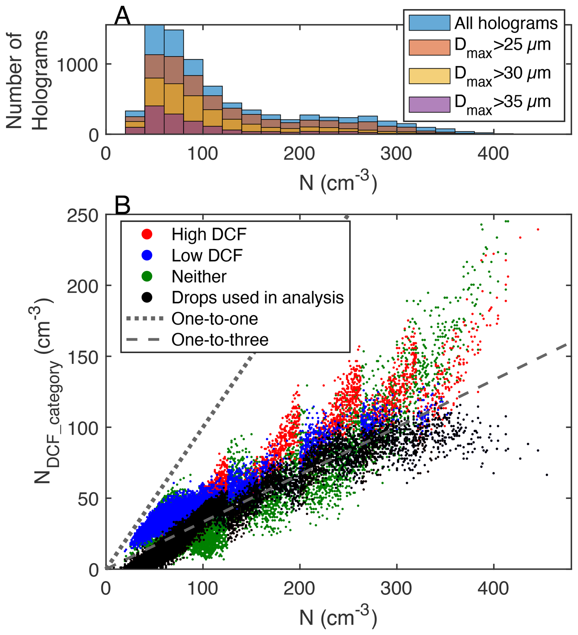
Figure A1 (A) Histogram of available holograms throughout the campaign. Different distributions account for holograms with different maximum drop diameters (D_max). (B) The number of droplets having high DCFs, low DCFs and DCFs meeting neither category in each hologram (N_{DCF_category}) related to their respective hologram's drop concentrations (N). Note that N refers to drop concentrations with D>12 µm.

Figure A1A shows the total number of holograms used in this study (blue bars). Since the focus of this study is on drops in the bottleneck drop size range, the total number of holograms with maximum drop diameters (D_max) > 25 µm, D_max > 30 µm and D_max > 35 µm are also provided to illustrate the number of available holograms used in the following analysis. Only holograms with D_max > 25 µm will be analyzed in this study.

Appendix B: Illustration of Monte Carlo-Hologram Comparison methodology

The Monte Carlo-Hologram Comparison methodology discussed here will follow step-by-step those listed in Table 3 (Sect. 3.2). Figure B1 shows multiple panels which aid in illustrating the methodology.

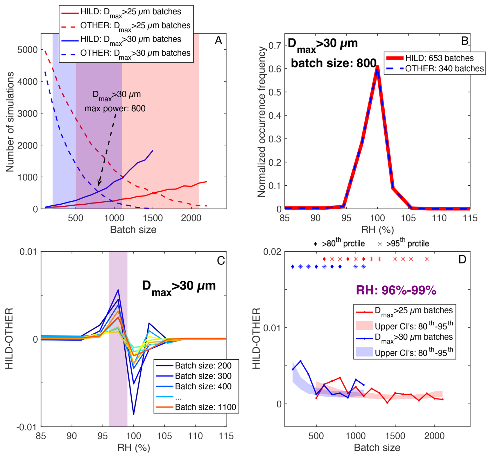
Figure B1 (A) Number of simulations in the HILD (solid lines) and OTHER (dashed lines) categories for all batch sizes. Results are shown for the D_max>25 µm (red lines) and D_max>30 µm (blue lines) datasets. Shading corresponds to batch sizes which are included in the analysis in Section 4.2 (following Step 4 in Table 3). (B) Normalized occurrence frequencies of RH samples shown from all HILD (red line) and OTHER (blue dashed line) simulations for the 800 hologram batch size from the D_max>30 µm dataset. (C) the difference of the HILD and OTHER normalized occurrence frequency over all RH bins in (B). Results are shown for all batch sizes from the D_max>30 µm dataset, where increasingly warmer lines correspond to larger batch sizes. (D) HILD – OTHER for the 96 %–99 % bin (purple shading in C) for all batch sizes included in the analysis. Results are shown for the D_max>25 µm (red line) and D_max>30 µm (blue line) datasets. The shading shows a range of confidence intervals, where the uppermost portion corresponds to the 95th percentile degree of significance and the lowermost portion corresponds to the 80th percentile. Uncertainty is determined using a permutation method, where samples are randomly sampled from the combined HILD and OTHER datasets 10 000 times.

This methodology incorporates a Monte Carlo sampling method in order to determine which holograms are associated with the isolated large drop trend. A number of holograms (i.e., batch) are sampled randomly 20 000 times from the available dataset. This is done for two datasets: (1) all holograms with D_max > 25 µm and (2) all holograms with D_max > 30 µm, to check for consistency in the reported trends. Since there is no prior information available for what number of holograms is contributing to the isolated large drop trend, we vary the number of holograms randomly selected (i.e., batch sizes), which range from 100 to 2200 holograms (Step 2 of Table 3). Each simulation is classified as either possessing the isolated large drop trend (HILD), or as not capturing this trend (OTHER). Conditions for these classifications are shown in Step 3 of Table 3, where percentiles are determined following the Monte Carlo-DCF methodology (Sect. 3.1). Note also that these conditions correspond to the same bottleneck drop size ranges as the large drop size bins from Figs. 4–6 (D= 25–50 µm).

Figure B1A shows the number of simulations meeting the HILD and OTHER classifications (solid and dashed lines, respectively) for the D_max > 25 and D_max > 30 µm datasets (red and blue lines, respectively) and for each batch size (x-axis). Results show the number of HILD (OTHER) simulations increases with increasing (decreasing) batch size. Note that the smallest and largest batch sizes have relatively few simulations meeting one of the categories. These simulations are not considered in the methodology since they have relatively low empirical power (i.e., number of simulations rejecting the null hypothesis divided by the total number of simulations), and only batch sizes having a minimum of 100 simulations meeting both categories are used in the analysis (Step 4 of Table 3). Batch sizes included in the analysis are shown by the red and blue shading for the D_max > 25 and D_max > 30 µm datasets, respectively. Note the arrow in Fig. B1A points to the batch size with the maximum empirical power for the D_max > 30 µm dataset (800), which will be referenced below.

To determine which conditions are associated with the isolated large drop trend, samples of a given variable are separately obtained from all the simulations in the HILD and OTHER categories. They are then combined to produce normalized frequency distributions for the two categories (Step 5 in Table 3). This is done for each batch size. For example, normalized frequency distributions of RH are shown for the HILD and OTHER simulations in Fig. B1B (red and dashed blue lines, respectively) for the 800 hologram batch size in the D_max > 30 µm dataset. The collocated RH samples are separately taken from all the holograms in the HILD simulations and all the holograms in the OTHER simulations, which include repeating samples. Due to the hypothesized impact of RH on the isolated large drop trend (discussed and validated in Sect. 4.1), we focus on RH for an exploratory analysis of the Monte Carlo-Hologram Comparison methodology. The distributions appear to be nearly identical due to the randomized hologram selection method, and the inability to discern which subgroup of holograms contribute to the HILD or OTHER trends and which holograms do not for any given simulation. However, differences in the HILD and OTHER normalized frequency distributions become apparent when taking their difference over each respective bin, which is shown in Fig. B1C. Differences in the normalized frequency distributions over the respective bins are shown for all batch sizes from the D_max > 30 µm dataset (i.e., batches within the blue shading in Fig. B1A), where smaller (larger) batch sizes have colder (warmer) lines.

Amongst all the batch sizes, there is a peak in the HILD – OTHER difference at RH of 96 %–99 % (purple shading). This is consistent with results in Fig. 4, where the isolated large drop trend is observed for subsaturated conditions. Figure B1D shows HILD – OTHER of the 96 %–99 % RH bin for all batch sizes, corresponding to the purple shaded bin of Fig. B1C. Unlike Fig. B1C, results from the D_max > 25 µm bin are also included (red line). Uncertainty bounds are also shown as the shaded coloring for the respective D_max datasets, where the upper boundary corresponds to the 95th percentiles and the lower boundary corresponds to the 80th percentiles. Uncertainty is determined using a permutation method where the same number of holograms are randomly selected from the combined HILD and OTHER simulations. For example, assume there are 300 holograms in the HILD category and 800 holograms in the OTHER category. 300 holograms will be randomly selected from the combined HILD and OTHER simulations (which would equal 1200 if there are no shared holograms between the HILD and OTHER simulations) and classified as HILD. Likewise, 800 holograms will be randomly sampled from the combined simulations and classified as OTHER. This is done 10,000 times for each batch size, and the difference of these two distributions is determined for all 10,000 permutations. This produces a range of differences used to discern statistical significance. Note that only 50 % (75 %) of differences for the D_max > 30 µm (D_max > 25 µm) batch sizes have differences exceeding the 95th percentile, seen by overlying stars above the respective batch sizes. Once again, this is likely due to the random selection of holograms and the inability to discern which samples are inherently associated with the isolated large drop trend in the HILD category, and likewise which holograms most strongly contribute to the OTHER trend. For this reason, the lower boundary of 80th percentiles are used in Sect. 4.2 to test for statistical significance.

Appendix C: Uncertainties and Sensitivity Tests

Due to multiple components involved in the methodology, numerous sensitivity tests were devised to test the robustness of the isolated large drop trend. Supplement Table S1 lists all such tests, and describes the rationale of the respective tests. Select uncertainties are further discussed here and are separately discussed for (1) uncertainties related to instrumentation and methodology and (2) uncertainties inherent in atmospheric phenomenon.

First considering uncertainty related to instrumentation uncertainty, the HOLODEC is associated with detection uncertainties of the spatial coordinates of drops: which are 0.001 cm in the x- and y-dimensions, and is maximized in the z-dimension (the longest dimension) at distances of 0.01 cm (Yang et al., 2005). However, 0.01 cm is precisely the interval range for incremental shell size increase, so uncertainties are not expected to significantly impact results. Errors may also be associated with droplets producing diffraction patterns that disturb those from closely neighboring drops, which may limit the detection of small drops within close proximity of larger drops. However, we suspect this is not a concern since the isolated large drop trend is primarily observed within holograms having low drop concentrations, where droplet pair distances are generally greater than for holograms having high drop concentrations.

The shell sizes are determined based on the HOLODEC sample volume size and consideration of drop concentrations in the sample environments. Specifically, maximum shell sizes are determined by considering the hologram sample volume size and the minimum shell sizes are determined by an intuitive consideration (i.e., crude consideration of counting statistics) that greater drop concentrations will allow increased resolution of DCF at smaller distances from the drops. Testing for different maximum shell sizes is particularly relevant since major trends discussed here occur at lower drop concentrations and for drops with the greatest isolation from neighboring drops (i.e., for the largest shell sizes). Unfortunately, increasing the shell size requires shrinking the guardrails which decreases the total number of available drops. Sensitivity tests where the maximum shell size is increased to 0.16 and 0.17 cm still capture the isolated large drop trend (not shown).

Shifting towards potential uncertainties related to cloud processes: similarly sized drops should follow similar trajectories, particularly drops within the stokes regime (D< ∼ 60 µm) where drop trajectories are partially a function of their size (Rogers and Yau, 1996). We can speculate that drops within this regime will be more likely to follow similar trajectories as similarly sized drops, and ultimately neighbor each other. This would result in smaller drops more likely to have neighboring drops, since these drops are more numerous than drops in the bottleneck range. Results evaluating the likelihood of drops having different sizes neighboring the inner drops (i.e., the likelihood of drop sizes within the shells of drops having a specified drop size range) is shown in Supplement Fig. S6. Evidence can be seen for drops neighboring those of similar sizes, particularly for drops having D∼ 20 µm (Fig. S6A). However, we suspect this is not a source of error/bias since if this were the case, the isolated large drop trend would also be observed (if not more likely observed) for holograms having high drop concentrations as well as those not limited to subsaturated environments. Further, the trend is observed at low drop concentrations where a greater number of similarly sized large drops are observed.

We suspect the largest uncertainty arises from the limited dataset of available holograms. Holograms available for the analysis are taken from twelve flight legs within nine research flights, and 75 % of the holograms are from four flight legs within two research flights. Another factor not explored here is the relation of these bottleneck trends to aerosol-cloud interactions. While broad aerosol characteristics can be determined for given flight legs, the inability to diagnose such characteristics in-cloud due to droplet contamination is a major limiting factor.