Regional and seasonal distribution of Arctic low-level cloud types and their relationship to large-scale environmental conditions

Low-level clouds strongly influence the Arctic surface energy budget and hydrological cycle, yet their representation in climate models remains challenging due to limited observations and complex interactions between local processes and large-scale conditions. This study analyzes eight years (2007–2016) of active remote sensing observations from CALIPSO and CloudSat to investigate the regional and seasonal distribution of four types of low-level clouds (between clutter height and 3000 m above ground level): warm liquid, ice-only, mixed-phase clouds (MPCs), and unglaciated supercooled liquid clouds (USLCs). 48 % of Arctic clouds occur at low altitudes. Statistical analysis of cloud-type occurrence shows that MPCs account for 17 %, ice-only clouds for 21 %, and USLCs for 8 %. This study provides a satellite-based assessment of USLCs over the Arctic, revealing occurrences of up to 20 % over marine regions during transition seasons. Multiple linear regressions are used to quantify the influence of key environmental drivers on the cloud type distribution. MPCs are linked to dynamically unstable conditions such as marine cold-air outbreaks, especially over open sea regions. USLCs preferentially develop under stable and relatively dry mid-tropospheric environments compared to ice clouds. Cloud–surface coupling shows that, on average, 17 % of low-level clouds are coupled to the surface. In winter, USLCs are more frequently coupled with the open ocean than with sea ice, emphasizing the strong thermodynamic control of the underlying surface. Ice-containing clouds are more frequently surface-coupled than USLCs. These results provide new insight into Arctic cloud-phase variability and offer guidance for improving their representation in large-scale models.

1 Introduction

Low-level clouds are ubiquitous in most regions of the Arctic (De Boer et al., 2009; Philipp et al., 2020; Taylor and Monroe, 2023; Wendisch et al., 2023a; Jiang et al., 2024). These clouds exert a strong influence on the surface energy budget, with an annual warming effect (Raschke et al., 2016; Li et al., 2023). The radiative effect of low-level clouds evolves strongly over time, yet differently if they are formed above the open ocean, sea ice-covered, or continental regions (Intrieri et al., 2002; Miller et al., 2015; Ebell et al., 2020; Yan et al., 2020; Cesana et al., 2024). Estimates of the seasonal and regional variability of the radiative effect of low-level clouds are still uncertain, as evidenced by the difficulty of simulating observations using current models (Lenaerts et al., 2017; Sedlar et al., 2020; Li et al., 2023; Griesche et al., 2024).

Local to large scale models struggle to simulate basic properties such as cloud cover and thermodynamic phase distribution in the Arctic (Prenni et al., 2007; De Boer et al., 2014; Komurcu et al., 2014; Cesana et al., 2015; McCoy et al., 2016; Pithan et al., 2016). In particular, climate models tend to underestimate the amount of liquid-containing clouds, which in turn leads to inaccurate estimates and variability of the CRE and precipitation (Tjernström et al., 2008; Vavrus et al., 2009; Cesana et al., 2012; Kay et al., 2016; McIlhattan et al., 2017). The discrepancy between model outputs and observations may be due to our lack of understanding of the complex processes involved in the formation of different cloud phases (droplets, crystals, and supercooled droplets) and their interplay with thermodynamical conditions, but also due to the difficulty in providing accurate and statistically representative observations of these different cloud phases. Modeling studies have shown that oversimplified or inaccurate parameterizations of microphysical processes (e.g., ice nucleation and droplet–ice interactions) can promote excessive freezing of supercooled droplets at low temperatures, thereby reducing the simulated liquid water content and leading to inaccuracies in cloud phase partitioning (Avramov et al., 2011; Ovchinnikov et al., 2014; Tan and Storelvmo, 2019). Earlier observational and modeling studies have demonstrated that the persistence of supercooled liquid droplets in Arctic mixed-phase clouds is governed by microphysical and dynamical processes rather than by temperature alone (Korolev and Isaac, 2003; Morrison and Pinto, 2005; Shupe et al., 2006; Ovchinnikov et al., 2014). More recently, Raillard et al. (2024) confirmed that the commonly used temperature-dependent phase partitioning in climate model cloud schemes is unable to sustain supercooled liquid water at low temperatures and therefore fails to accurately simulate Arctic mixed-phase clouds (MPCs). The life cycle of these low-level clouds results from complex interactions between local microphysical, radiative, dynamical processes, and larger-scale environmental conditions (Morrison et al., 2012; Li et al., 2020a, b; Griesche et al., 2021). Recent developments in cloud microphysics and turbulence parameterizations (Raillard et al., 2024; Vignon et al., 2026), as well as the increasing use of observational constraints and process-oriented model evaluation (Kay et al., 2016; Tan and Storelvmo, 2019), have led to measurable improvements in the representation of Arctic clouds in both regional and global models. Therefore, continued synergy between long-term observations, targeted field campaigns, and model development is essential to further reduce uncertainties in Arctic cloud processes and their radiative effects.

Statistics of ground-based observations have played a central role in characterizing Arctic low-level cloud properties. They have highlighted the high occurrence of low-level clouds and the persistence of liquid-containing clouds, which exert a strong influence on the surface energy budget (Dong et al., 2010; Shupe et al., 2011; Nomokonova et al., 2019; Ebell et al., 2020). By providing vertically resolved measurements of cloud structure and thermodynamic phase at high temporal resolution, ground-based observations have enabled detailed investigations of the microphysical and dynamical processes controlling the formation and maintenance of mixed-phase clouds. These long-term observations from fixed observatories have substantially increased our understanding of the physical processes that govern the life cycle of low-level clouds. Airborne observations have provided a valuable complement to ground-based measurements by offering targeted snapshots of cloud structure and microphysical properties over a broader spatial extent (Wendisch et al., 2019; Mech et al., 2022; Wendisch et al., 2024). However, these campaigns are inherently limited in duration and sampling frequency and therefore mainly capture specific meteorological conditions. As a result, despite the significant advances brought by both ground-based and airborne observations, their findings remain representative of specific locations and cannot be directly extrapolated to the entire Arctic domain.

Long-term satellite observations of the regional and seasonal distribution of low-level cloud types are therefore crucial to reduce the spread among large-scale models on the annual cycle of the cloud fraction and cloud phase (Lenaerts et al., 2017; Taylor et al., 2019). Studies based on satellite observations have shown pronounced inter-regional and seasonal variations of the low-level cloud occurrence (Lelli et al., 2023; Jiang et al., 2024), yet with a lack of coherence, especially regarding the retrieval of the cloud phase. Passive remote sensing observations have well-known limitations in the Arctic, leading to an underestimation of the low-level and mixed-phase cloud fraction (Schweiger and Key, 1992; Chan and Comiso, 2013; Philipp et al., 2020). Satellite products based on active remote sensing observations of the vertical structure of clouds improved the characterization of the distribution of the cloud phase in the Arctic (Cesana et al., 2012; Mioche et al., 2015; Matus and L'Ecuyer, 2017; Cesana et al., 2024).

From a satellite-based observational perspective, disagreements persist when comparing basic properties such as the occurrence of the thermodynamic phase of low-level clouds with active instruments. This is partly due to the ability of the instruments (lidar and radar) used to detect the particular microphysical structure of low-level MPCs, which generally consist of an upper layer dominated by supercooled water droplets and lower layers containing ice crystals (Shupe et al., 2006; McFarquhar et al., 2007; Mioche et al., 2017; Moser et al., 2023). Because the space-based lidar cannot penetrate most of the optically thick liquid-topped layers, studies relying on the space lidar alone tend to combine real MPCs and liquid-only clouds into a single liquid-containing cloud type. Cloud phase retrievals based on algorithms that exploit the lidar-radar synergy can reduce these biases, but they are also confronted with the observational scale-dependent definition of a mixed-phase cloud. Indeed, in most of the studies, clouds are considered to be in the mixed-phase regime only if both liquid droplets and ice crystals are detected in the same cloud layer or pixel. This assumption is expected to lead to an underestimation of the MPCs occurrence as these clouds are often characterized by successive single-phase layers, and only one layer can be detected by a single instrument. Despite these advances, a consistent Pan-Arctic characterization of the thermodynamic phase of low-level clouds and its regional and seasonal variability remains limited, particularly when considering long-term statistics derived from a uniform methodology. Therefore, as a first step, it is important to more accurately assess the frequency of occurrence of different low-level cloud types related to their thermodynamic phase. In addition to ice clouds and warm liquid clouds, a segregation between MPCs and unglaciated supercooled liquid clouds (USLCs) is necessary, but has been lacking in previous studies. Most satellite-based climatologies do not explicitly distinguish between MPCs and USLCs, although these cloud types arise from different microphysical processes and are expected to respond differently to large-scale environmental conditions. In a warmer and wetter Arctic setting, the cloud-type regional and seasonal distributions are expected to change, and long-term observations of cloud vertical profiles are needed to monitor and capture possible modifications of the Arctic cloudiness.

Spaceborne cloud phase observations combined with regional reanalyses can be exploited to identify factors influencing the distribution of cloud types at larger spatial and temporal scales. Previous studies have shown that lower tropospheric stability (LTS), the vertical structure of temperature and humidity, moisture inversions, air mass intrusions, long-range transport of aerosols, and surface type are among the main factors controlling the low-level cloud cover (Sedlar et al., 2012; Coopman et al., 2018; Knudsen et al., 2018; Pithan et al., 2018; Eirund et al., 2019). For instance, Yu et al. (2019) showed that strong LTS over open ocean tends to increase the cloud cover and the amount of liquid water, whereas the opposite trend seems to be observed over sea ice (Taylor et al., 2015). The large-scale advection of moisture and heat often associated with phenomena such as warm air intrusions (WAI) or cold air outbreaks (CAO) from higher or lower latitudes can also induce rapid changes in local weather conditions and directly affect the formation and structure of low-level clouds (Lackner et al., 2023). Moisture intrusions over the boundary layer are usually associated with increased cloudiness (Persson et al., 2017; Messori et al., 2018) and tend to promote larger liquid water content (Eirund et al., 2019). However, during WAI over the oceanic boundary layer, there seems to be no consensus on its impact on low-level cloud microphysical properties and coverage. Some studies show a decrease in cloud fraction and liquid water content (Knudsen et al., 2018; Eirund et al., 2019) while in situ observations point towards an increase in number and mass concentrations of liquid water droplets (Mioche et al., 2017; Moser et al., 2023). The underlying surface and whether the cloud is coupled or decoupled from the surface, as well as the large-scale transport of aerosol particles, also modify the microphysical properties and the thermodynamic phase of low-level clouds (Kay and Gettelman, 2009; Bossioli et al., 2021; Schmale et al., 2021; Raut et al., 2022; Moser et al., 2023). In general, the regional variability of these environmental factors is not well represented in climate models, which impacts the simulation of the distribution of the low-level cloud properties in the Arctic (Barton et al., 2014; Cesana et al., 2015; McCoy et al., 2016; Tan et al., 2016).

Moreover, in the context of significant changes in this region of the globe, low-level cloud fractions and types may be affected by changes in large-scale environmental conditions (Kay and Gettelman, 2009; Eastman and Warren, 2010; Liu et al., 2017; Morrison et al., 2019; Liu and Schweiger, 2024). To improve our understanding of how these conditions influence the properties of low-level clouds and to reduce model biases, we argue that more accurate estimates of the frequency of occurrence of phase-related cloud types are necessary in different regions of the Arctic. The first objective of this study is to provide representative and longer-term statistics on the regional and seasonal distribution of low-level warm liquid, ice-only, and mixed-phase clouds, as well as the overlooked unglaciated supercooled liquid clouds. By explicitly distinguishing these cloud types, this study aims to better constrain the contribution of liquid-containing clouds to the Arctic cloud climatology. The second objective of this study is to identify a first set of basic environmental parameters that impact the geographical distribution of cloud-type occurrence at a large scale. Statistical analyses of the relationship between cloud-type cover and these parameters provide insight into which are the most influential parameters on the low-level cloud cover at a regional scale. This data set and its associated analyses can be used to evaluate the output of climate and regional models, provide guidance on improving cloud phase parameterization, and facilitate future comparisons with Earth Clouds, Aerosols, and Radiation Explorer (EarthCARE; Illingworth et al., 2015) observations of cloud distribution in the Arctic.

We rely on the synergy of CALIPSO (Cloud-Aerosol Lidar and Infrared Pathfinder Satellite Observations) and CloudSat radar satellite measurements (DARDAR-MASK products; Delanoë and Hogan, 2008, 2010; Ceccaldi et al., 2013) collocated with thermodynamic variables from ECMWF (European Centre for Medium-Range Weather Forecasts) analyzes and sea ice concentration to analyze 8 years of cloudy scenes over different Arctic regions. DARDAR (raDAR–liDAR) products, combined with the cloud classification algorithm, are used to determine the occurrence of the thermodynamic phase of low-level clouds. This study focuses on providing long-term, regionally resolved statistics of low-level cloud thermodynamic phases and on identifying the dominant large-scale environmental parameters associated with their occurrence. Section 2 describes the dataset, the DARDAR classification algorithm, and the statistical analyzes used to characterize cloud-type occurrences. The uncertainties and limitations associated with this methodology are also discussed. Section 3 presents the results on the spatial distribution and temporal variations of cloud-type occurrences. Multiple linear regressions (MLR) are also implemented to quantify the influence of key environmental parameters on cloud occurrences. In particular, we identify the dominant parameters driving each cloud-type and examine their relationship with cloud–surface coupling. In Sect. 4, we discuss the main results in the context of previous studies.

2 Methods and Data

2.1 DARDAR products and cloud-type classification

This study investigates the regional and seasonal variability of cloud occurrence, located below 3000 m above ground level (a.g.l.), in the Arctic (60–82° N) between 2007 and 2016 using the DARDAR-MASK v2.23 product (Delanoë and Hogan, 2008, 2010; Ceccaldi et al., 2013). In this satellite product, the vertical profiles of the 532 nm attenuated backscatter coefficient measured by the CALIOP lidar onboard CALIPSO (McGill et al., 2007; Winker et al., 2007) are merged with the 94 GHz (W-band) reflectivity profiles from the Cloud Profiling Radar (CPR) onboard CloudSat (Stephens et al., 2002) on the same resolution grid. Since the lidar signal is more sensitive to the cloud optical extinction and the radar reflectivity to the size of large cloud particles (ice crystals), the combination of both measurements is used to detect the hydrometeor type (or phase) within a cloud layer. Therefore, the DARDAR-MASK v2.23 product provides a vertically resolved classification of the cloud hydrometeor type and aerosols (see Fig. S1 in the Supplement) along the A-Train track, with each atmospheric pixel (60 m × 1.7 km) assigned to one of 18 classes (Ceccaldi et al., 2013). These classes include clear sky, aerosols, stratospheric features, and several categories of hydrometeors.

Warm liquid water pixels are identified by strong lidar attenuation (${\mathit{\beta }}_{\mathrm{532}}\ge \mathrm{2}\times {\mathrm{10}}^{-\mathrm{5}}$ m⁻¹ sr⁻¹) at temperatures above 0 °C. Supercooled liquid water pixels are defined by subfreezing temperatures (−40 °C < T < 0 °C), along with strong lidar attenuation, and for a layer thickness lower than 360 m (Hogan et al., 2004; Zhang et al., 2010). Mixed-phase pixels are characterized by a strong lidar attenuation caused by supercooled liquid droplets combined with the presence of ice crystals detected by the radar reflectivity signal. All remaining cloudy pixels at below-freezing temperatures are classified as ice-only when the lidar backscatter at 532 nm is weak (${\mathit{\beta }}_{\mathrm{532}}<\mathrm{2}\times {\mathrm{10}}^{-\mathrm{5}}$ m⁻¹ sr⁻¹), indicating no strong lidar attenuation, or when a radar detection signal is measured (CloudSat radar mask values > 30 were considered as cloud detection; Ceccaldi et al., 2013); these conditions may occur simultaneously and are both indicative of ice-only clouds.

It should be noted that the lidar signal can be rapidly attenuated in clouds with an optical depth greater than 3 to 5, depending on their microphysical composition (Chepfer et al., 2014). If the signal is extinguished or fully attenuated, the underlying cloud pixel phase diagnosis relies only on the radar reflectivity. Backscattering signals from spaceborne cloud radars are known to be affected by surface returns such as ground clutter or false ground detection. This can result in the misclassification of hydrometeors in the lowest atmospheric layers (Marchand et al., 2008). Previous studies have shown that the vertical extent of the CloudSat CPR blind zone varies greatly depending on the surface type. It is narrow over open ocean and sea ice (approximately 750 m) but can extend up to approximately 1.2 km over land (Maahn et al., 2014; Schirmacher et al., 2023). The DARDAR-MASK product includes dedicated classes to identify potential contamination by clutter (class −1: surface and subsurface), thus reducing classification biases close to the surface. In Mioche et al. (2015), the impact of radar clutter was reduced by setting a lower-altitude threshold of 500 m. This threshold was determined through comparisons with a limited set of ground-based observations. However, this fixed threshold does not adequately account for surface-dependent radar contamination, especially over land.

In this study, the lower limit of the analysed cloud layer is no longer fixed. Instead, the altitude of the lowest possible detectable cloud layer is individually determined for each CloudSat profile, based on the height of the radar clutter. This adaptive approach explicitly accounts for variations in surface elevation and terrain complexity, ensuring consistent cloud detection over the ocean, sea ice, and land. Consequently, the cloud occurrence results presented in this study correspond to clouds detected between the radar clutter height and 3000 m (a.g.l.). A dedicated statistical analysis of clutter height distributions categorized by surface type shows median clutter heights of approximately 660 m over open ocean and sea ice, and 830 m over land (see Fig. S2 and Table S1 in the Supplement).

DARDAR-MASK pixel classification issues were also reported by Mioche and Jourdan (2018). Comparisons with co-located in situ observations in low-level Arctic clouds showed that the liquid or the ice phases were accurately diagnosed by DARDAR-MASK 90 % of the time in single-phase clouds. However, in situ measurements revealed that almost 50 % of the DARDAR-MASK “ice” pixels within boundary layer mixed-phase clouds were actually a mixture of supercooled water droplets and ice crystals. The main sources of disagreement were attributed to the full attenuation of the lidar signal by the upper cloud layers and the contamination of near-surface pixels by radar ground echo.

To mitigate these limitations, we used the DARDAR classification program to estimate the occurrence of five distinct types of clouds. This program was originally developed for Arctic clouds by Mioche et al. (2015) and later updated and extended by Bazantay et al. (2024) to study low-level clouds over the Southern Ocean, hence the name DARDAR-SOCP (DARDAR for Southern Ocean Cloud Phase). The algorithm analyzes the vertical structure of each atmospheric column to extract the cloud composition between clutter height and 3000 m (a.g.l.). The atmospheric column sampled is divided into “pixels” with a vertical resolution of 60 m, which are all assigned to a specific DARDAR-MASK class value. A cloud is defined as at least three vertically adjacent cloudy pixels (180 m), in accordance with in situ observations of low-level clouds (Mioche et al., 2017; Achtert et al., 2020; Järvinen et al., 2023; Moser et al., 2023; Zanatta et al., 2023). A single column may contain several distinct cloud layers, provided that they are separated by at least three clear-sky pixels. Accordingly, low-level clouds are first separated into two broad thermodynamic categories: warm clouds (T > 0 °C) and cold clouds (T ≤ 0 °C). Within the cold-cloud category, three phase-based subcategories are further distinguished: ice clouds, unglaciated supercooled liquid clouds (USLCs), and mixed-phase clouds (MPCs), which are described below:

• Warm clouds: consisting exclusively of liquid water droplets at T > 0 °C.

• Cold clouds: including all cloud types with temperatures below 0 °C (i.e., all clouds except warm clouds).

• Ice clouds: composed entirely of pixels of ice crystals.

• Unglaciated supercooled liquid clouds (USLCs): composed solely of supercooled liquid water droplet pixels.

• Mixed-phase clouds (MPCs): characterized by a mixture of pixels of different phases (i.e., pixels of liquid water droplets and pixels of ice crystals and/or droplets and crystals in the same pixel).

Due to the CloudSat CPR's coarse vertical resolution, very weak ice precipitation, which is commonly observed in stratiform mixed-phase clouds, may remain undetected. Furthermore, without Doppler velocity measurements, the cloud radar cannot reliably distinguish between cloud ice and snow. Consequently, all radar-detected frozen hydrometeors fall into a single ice category within the DARDAR classification framework. Additionally, the lowest observable altitude is determined by the changing height of the radar clutter. Ice precipitation occurring entirely below this level cannot be detected, which could lead to an overestimation of the occurrence of USLCs. To assess this effect, we distinguish between USLCs that overlap the height of the clutter and those that do not. As the majority of identified USLCs (80 %) do not overlap with the clutter, the potential bias associated with undetected low-level ice precipitation is expected to remain limited (see Fig. S3 in the Supplement). Furthermore, although liquid-phase precipitation is not explicitly included in the classification, it is implicitly incorporated into the warm-cloud category. Drizzle can also occur in supercooled liquid containing clouds. Drizzle-sized liquid drops and falling ice crystals are expected to produce similar radar reflectivity signatures. Therefore, ambiguity in phase attribution is inherent when relying on spaceborne active sensors, particularly under conditions of lidar attenuation.

In DARDAR-SOCP, the requirement of at least three consecutive cloudy pixels to define a cloud can bias the detection of mixed-phase clouds, which often consist of successive single-phase layers. As a result, the occurrence of MPCs can be overestimated compared to the occurrence of ice and liquid clouds. We showed that these cloud-type classification issues lead to systematic biases in cloud occurrence of about 15 % for ice, 20 % for liquid, and 10 % for mixed-phase clouds (see Supporting Information of Bazantay et al., 2024). A potential underestimation of liquid phase may also occur as a result of lidar signal attenuation by an overlying liquid water layer located above 3000 m. The cloud occurrence for each type (OC_n) is calculated as the ratio of the number of observations of that type (N_n) to the total number of satellite footprints (N_footprint), expressed as a percentage:

$$\begin{array}{}\text{(1)}& {\mathrm{OC}}_n={\displaystyle \frac{N_n}{N_{\mathrm{footprint}}}}\times \mathrm{100}\end{array}$$

Cloud occurrences are computed for each cloud type on the basis of 1 d satellite data averages, ensuring statistical robustness at a regional scale. All footprints located between 60 and 82° N (14 overpasses per day in the Arctic region) are processed and aggregated into 1° × 1° latitude–longitude boxes. The years 2011 and 2012 are excluded due to an anomaly in the CloudSat battery, which caused data loss. Before 2010, both daytime and nighttime observations were used, while after 2012, only daytime observations were considered in our study because of the same battery-related issues. Relying only on CloudSat's daylight operations mode (2013–2016) led to fewer observations, particularly during winter and at high latitudes (Kotarba and Solecki, 2021). This limitation introduces a seasonal bias in cloud climatologies, with a slight overestimation of winter occurrences (≈5 %), especially over oceans (Noel et al., 2018). More details are provided in the Supplement (see Figs. S4, S5, and Sect. S1).

2.2 Comparison with ground-based data

As explained in the previous section, it is well known that CloudSat observations and thus the DARDAR product may be affected by a blind zone near the surface due to radar ground echoes. As previous studies based on ground and airborne observations have highlighted the prevalence of Arctic clouds near the surface, it is important to evaluate whether and to what extent the DARDAR cloud occurrences presented here are underestimated. To this end, an independent evaluation of DARDAR cloud occurrences has been conducted, based on comparisons with ground-based data from the Cloudnet network. Cloudnet observations based on multi-remote sensing instruments are used to produce a “classification product” that includes different cloud types (Hogan et al., 2004, for details). This product is comparable to the DARDAR product used in this study. We use Cloudnet classification products from the Ny-Ålesund (Norway, 78°55^′ N, 11°56^′ E) and the Hyytiälä (Finland, 61°84^′ N, 24°28^′ E) Arctic sites, as they are the only ones in the Arctic that were available for a significant period (several months) when CALIPSO and CloudSat were operational (June to December 2016 at Ny-Ålesund and March to August 2014 at Hyytiälä). To ensure representative occurrences comparable to ground-based observations, DARDAR cloud occurrences have been calculated in a square of 5° of latitude by 5° of longitude (±2.5° in both latitude and longitude), centered over each ground site location.

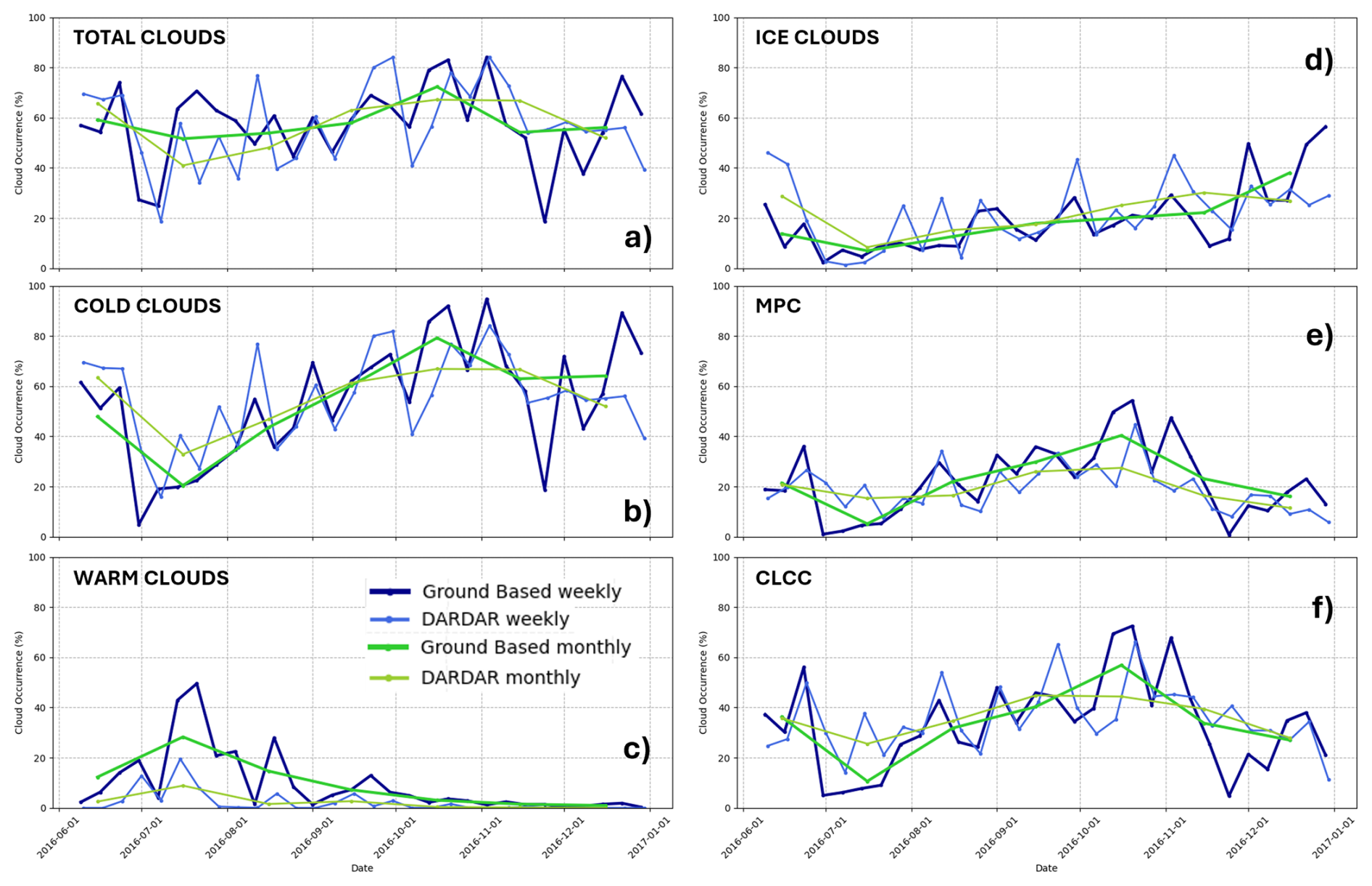
Figure 1 Comparison of DARDAR and ground-based observations of: (a) total, (b) cold, (c) warm, (d) ice, (e) mixed-phase, and (f) cold liquid-containing cloud occurrence up to 3000 m above ground level at Ny-Ålesund (78°55^′ N, 11°56^′ E). Weekly (blue) and monthly (green) occurrences are shown. Ground-based observations are represented by thicker, darker lines.

The results for the Ny-Ålesund site are shown in Fig. 1 (Results for the Hyytiälä site are provided in Fig. S6 in the Supplement). In this figure, occurrences of total (Fig. 1a), cold (Fig. 1b), warm (Fig. 1c), ice (Fig. 1d), mixed-phase (Fig. 1e) and cold liquid-containing (Fig. 1f) clouds in the altitude range up to 3000 m above ground level are presented. Weekly (blue colors) and monthly (green colors) occurrences have been computed. Ground-based occurrences are displayed in thick straight lines. We note that the last cloud type (CLCC for cold liquid-containing clouds) was only computed for this evaluation. The supercooled liquid class is not included in the Cloudnet classification product. Consequently, the USLCs class could not be evaluated directly. However, to be coherent with the Cloudnet product, cold liquid-containing clouds, including USLCs and MPCs cloud types, have been computed from DARDAR data.

Generally, a good level of consistency is observed when comparing ground-based and space-based occurrences. The weekly and monthly variability are very similar for both observation sites. However, differences are observed in the values of cloud occurrences, particularly those averaged over a week. These differences may be due to the blind zone, which could affect the satellite products. This could explain the higher frequency of cloud occurrences retrieved from ground-based instruments. However, these discrepancies may also be due to the effect of averaging occurrences within a 5 × 5° box. To quantify the differences, the average difference was calculated (see Table S2 in the Supplement). The average differences between ground-based and spaceborne cloud occurrences remain very small at only a few percent and are evenly distributed around zero (ranging from −5.8 % to +5.2 %, as can be seen in Fig. 1). This indicates that there is no bias, meaning that occurrences are neither under- or overestimated. The standard deviations show non-negligible values (up to 23 %). Therefore, the main source of uncertainty is probably the spatial representativeness of the data (i.e. the comparison of a 5 × 5° box to a single location) rather than the blind zone. Thus, the general good agreement between the two datasets with no systematic bias leads to the conclusion that the impact of ground clutter on the low-altitude cloud occurrences from DARDAR presented in the paper remains limited.

Table 1 List of the environmental parameters.

2.3 Selection of environmental factors

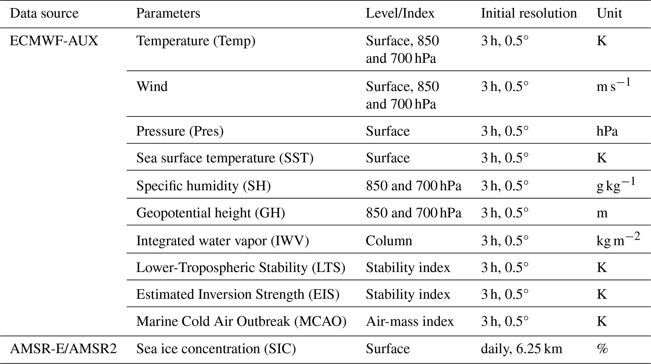
Thermodynamic data are used to analyze the impact of environmental conditions on cloud occurrence and type. DARDAR-SOCP retrieves thermodynamic variables from ECMWF analyzes, which are integrated into DARDAR-MASK files as part of the ECMWF-AUX collocated products (Delanoë et al., 2011; Hersbach et al., 2020). ECMWF-AUX is an intermediate product in which the 3 h thermodynamic property forecasts of the ECMWF model on a 0.5° × 0.5° grid are interpolated to each CPR radar profile (Cronk and Partain, 2017). The set of parameters used in this study is summarized in Table 1. In addition, three metrics are calculated to characterize the vertical structure of the lower troposphere and the advection of heat and moisture at a regional scale:

• Lower-Tropospheric Stability (LTS; Wood and Bretherton, 2006) is defined as the potential temperature difference between the free troposphere and the surface:

  $$\begin{array}{}\text{(2)}& \mathrm{LTS}={\mathit{\theta }}_{\mathrm{700}\mathrm{hPa}}-{\mathit{\theta }}_{\mathrm{surf}}\end{array}$$

  LTS provides a bulk measure of static stability across the lower troposphere and has been widely used as a large-scale predictor of low-level cloudiness (Zhang et al., 2009; Taylor and Monroe, 2023). Under Arctic conditions, where low-level clouds often reside well below 700 hPa, LTS primarily reflects the thermodynamic contrast between the cloudy boundary layer and the overlying free troposphere, rather than the stability within the cloud layer itself, and low LTS values should not be interpreted as convective instability.

• Estimated Inversion Strength (EIS), originally proposed by Wood and Bretherton (2006), provides a more physically meaningful estimate of the inversion strength at the top of the boundary layer. EIS refines the LTS by correcting for the moist-adiabatic temperature structure below the inversion:

  $$\begin{array}{}\text{(3)}& \mathrm{EIS}={\mathit{\theta }}_{\mathrm{700}\mathrm{hPa}}-{\mathit{\theta }}_{\mathrm{surf}}-{\mathrm{\Gamma }}_{\mathrm{m}}^{\mathrm{850}\mathrm{hPa}}(Z_{\mathrm{700}}-\mathrm{LCL})\end{array}$$

  where ${\mathrm{\Gamma }}_{\mathrm{m}}^{\mathrm{850}\mathrm{hPa}}$ is the moist-adiabatic lapse rate evaluated at 850 hPa, Z₇₀₀ is the geopotential height of the 700 hPa level, and LCL is the lifting condensation level height. Larger EIS values indicate a stronger inversion, which limits entrainment from the overlying free troposphere and promotes the persistence of low-level clouds (Naud et al., 2023).

• The Marine Cold Air Outbreak index (MCAO; Fletcher et al., 2016) reflects the effects of cold-air advection and air–sea interaction. This index is calculated over oceanic regions and defined as the potential temperature contrast between the ocean surface and the lower troposphere at 800 hPa:

  $$\begin{array}{}\text{(4)}& \mathrm{MCAO}={\mathit{\theta }}_{\mathrm{skin}}-{\mathit{\theta }}_{\mathrm{800}\mathrm{hPa}}\end{array}$$

  Positive MCAO values indicate that cold air is advected over a relatively warm surface. It is associated with enhanced turbulent heat and moisture fluxes, increased boundary-layer mixing, and convective cloud development (Slättberg et al., 2025). While LTS and EIS describe primarily static atmospheric stability, MCAO accounts for dynamically driven processes linked to synoptic-scale circulation (Fletcher et al., 2016). MCAO is a useful indicator of low-level cloud occurrence during cold-air outbreak (CAO) and warm-air advection (WAA) conditions.

In this study, we also account for the type of surface underlying the cloud: land, open ocean, or sea ice. In particular, sea ice concentration (SIC) is used to characterize sea and ocean surface conditions. SIC data are obtained from the AMSR-E instrument on board AQUA (2002–2011) and AMSR2 on board GCOM-W1 (2012–present). Both are passive microwave radiometers that measure brightness temperatures in several channels (18–89 GHz). SIC is retrieved with the ARTIST Sea Ice (ASI) algorithm (Spreen et al., 2008; Du et al., 2017), which has been validated against other retrieval methods and in situ data (Wiebe et al., 2009). The typical uncertainty for 100 % sea ice cover is 5.7 % (Spreen et al., 2008), with higher uncertainties in the marginal ice zone due to mixed ocean/ice pixels and atmospheric contamination.

The selection of this limited set of environmental factors is consistent with previous studies carried out in mid-latitudes (Scott et al., 2020; Naud et al., 2023) and in the Arctic (Morrison et al., 2012; Kay et al., 2016; Liu et al., 2017; Yu et al., 2019). The environmental parameters are averaged over 1 d and collocated on a 1° × 1° grid to match the temporal and spatial resolution used for cloud-type occurrences. The environmental parameters are partitioned in the same way as cloud-type occurrences to ensure temporal consistency. This timescale is thus appropriate both to obtain representative cloud-type occurrences and to investigate the variability of environmental parameters at the regional scale.

2.4 Multiple linear regression

In this study, we implement multiple linear regression (MLR) analyzes to identify the environmental factors that contribute the most to the regional and seasonal variability of cloud-type occurrences. This statistical approach is used to predict the variation of a dependent variable (e.g., cloud occurrence) as a linear combination of several explanatory variables (e.g., environmental parameters). It relies on a least-squares estimator to minimize the error between predicted and observed values (Legendre and Legendre, 2012). In this study, we apply MLR to relate several environmental predictors to the target variable (OC_n) as follows:

$$\begin{array}{}\text{(5)}& {\mathrm{OC}}_n={\mathit{\beta }}_{\mathrm{0}}+{\mathit{\beta }}_{\mathrm{1}}{x}_{\mathrm{1}}+\mathrm{\dots }+{\mathit{\beta }}_i{x}_i+\mathit{ϵ}\end{array}$$

where β₀ represents the intercept, β_i the regression coefficients associated with each predictor x_i, and ϵ the residual. MLR variables (x_i) are normalized to ensure a direct comparison of the relative importance of each parameter (Bring, 1994; Grace et al., 2018). We follow the same MLR methodology as in Coopman and Tan (2023), ensuring consistency with recent approaches applied to Arctic cloud studies. Before each regression, we evaluated the multicollinearity between predictors and explanatory variables based on the Variance Inflation Factor (VIF, see Fig. S7a in the Supplement). According to Liu et al. (2021), variables with a VIF greater than 10 are excluded from multiple linear regression analysis. Non-significant predictors, either showing a p-value greater than 0.05 or exhibiting no clear influence (e.g., wind; see Fig. S7b in the Supplement) in the simple correlations with cloud-type occurrences (R²<0.1), were excluded to retain only robust explanatory factors for each cloud type. The relation between the cloud occurrence and the environmental parameters is expected to be nonlinear, leading to a relatively low R², but it remains satisfactory at the first order with R² greater than 0.3. To assess potential dependencies between predictors, we also computed pairwise correlations using Spearman's rank method. The correlation matrix shown in Fig. 2 reveals strong links between several environmental variables that are inherently interdependent and are often correlated to varying degrees. This is especially the case for the temperature variables ($R_{\text{Surf\_Temp/Temp\_850hPa}}^{\mathrm{2}}=\mathrm{0.88}$; Fig. 2) and the humidity variables at different atmospheric levels, as well as for EIS and LTS ($R_{\text{EIS/LTS}}^{\mathrm{2}}=\mathrm{0.91}$; Fig. 2).

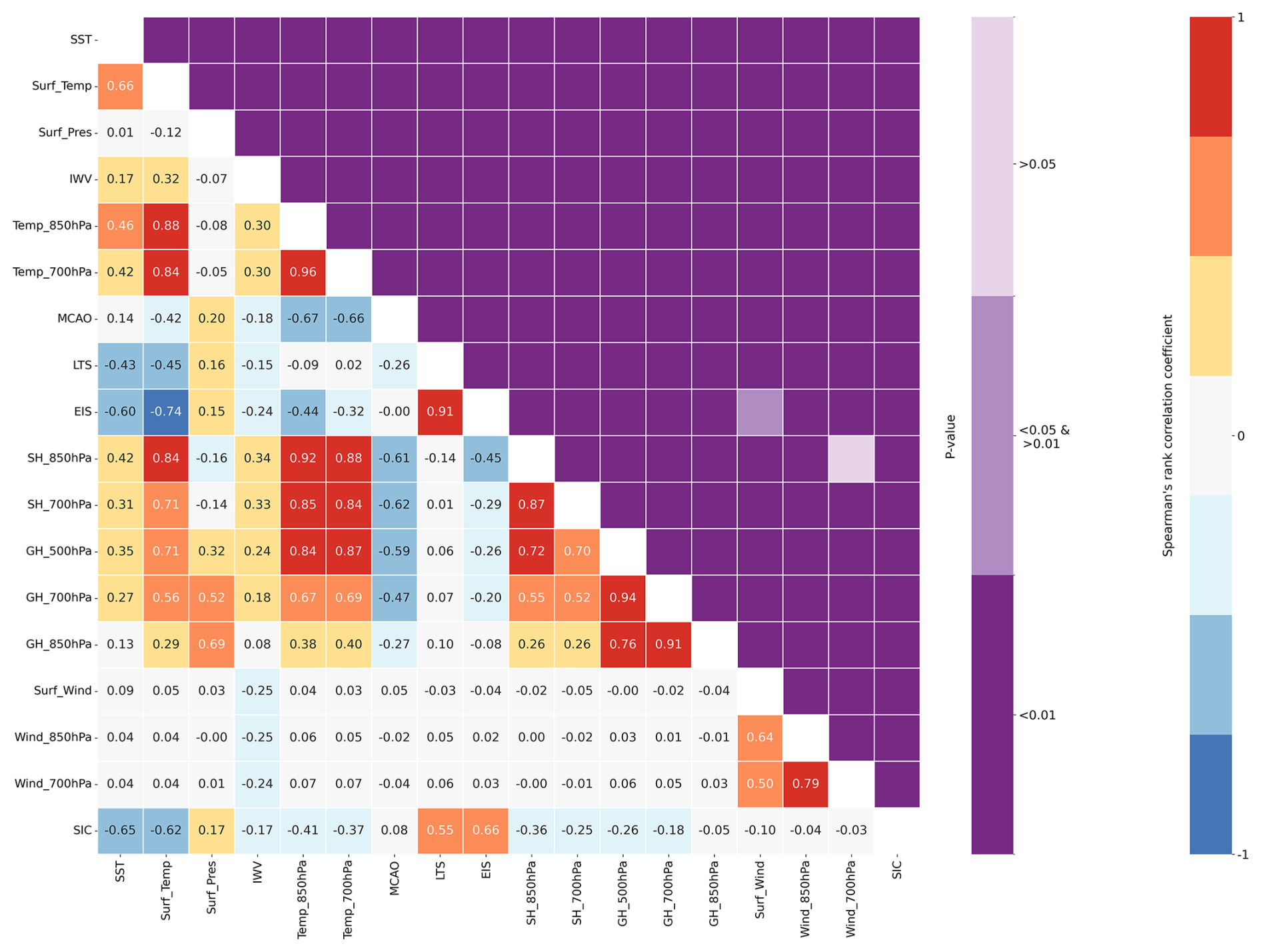
Figure 2 Spearman's rank correlation matrix and associated p-values for each key parameter across all regions.

Accordingly, to minimize the collinearity and redundancy between the different predictors, eight variables are selected for the MLR analyzes: surface temperature (Surf_Temp), surface pressure (Surf_Pres), integrated water vapor (IWV), lower-tropospheric stability (LTS), marine cold air outbreak (MCAO), specific humidity at 700 hPa (SH_700hPa), geopotential height at 850 hPa (GH_850hPa), and sea ice concentration (SIC). For MLR, LTS was preferred over EIS because it exhibits weaker correlations (than EIS, Fig. 2) with the other predictors, thereby reducing multicollinearity within the MLR framework. Some thermodynamic parameters cannot be computed over all regions (e.g., LTS over high-elevation areas such as central Greenland); grid cells with missing parameter values are therefore excluded from the MLR analysis. These parameters characterize the basic properties of the lower troposphere thermodynamic structure and the surface conditions. We expect this limited set of parameters to be sufficient to statistically investigate how varying environmental conditions impact the regional distribution of low-level clouds.

During the eight-year study period, the observational dataset used in the MLR analysis consists of approximately 2 450 300 data points distributed across 1° × 1° grid cells. However, some low-latitude grid cells can sometimes contain a limited number of observations. This makes the calculation of cloud occurrence frequencies and associated statistics less robust. To ensure adequate sampling, a minimum sampling threshold for the number of observations per grid cell is defined based on the first quartile (Q1) of the distribution of daily observations in the lowest latitude band (60–61° N), where sampling is weakest. We find a Q1 value equal to 12 observations per day. Therefore, only 1° × 1° grid cells containing at least 12 DARDAR pixels per day are retained in the cloud occurrence and MLR analyses.

The remaining dataset is randomly divided into two subsets. 80 % of the data are used to train the MLR models, and the remaining 20 % serve as an independent test set for validation. The performance of the regression model is quantified using the coefficient of determination (R²). In addition, the statistical significance of each regression coefficient is assessed using a Student's t-test, and the corresponding p-values are reported for all predictors. These metrics provide a measure of the precision and robustness of the regressions.

2.5 Surface-coupling state

The cloud–surface coupling state is determined from the thermodynamic structure of individual cloud profiles. Building on the work of Gierens et al. (2020), who introduced a simplified version of the coupling algorithm originally proposed by Sotiropoulou et al. (2014), we analyze the vertical profile of the potential temperature (θ) from the cloud liquid layer base to the surface. The cumulative mean of θ is computed for each individual cloud profile over this layer and compared to the local θ profile. A cloud profile is classified as decoupled from the surface if the difference between the mean θ and the instantaneous θ exceeds 0.5 K at any level. Cloud profiles that do not exceed this threshold are considered to be related to surface-coupled clouds. For ice-only clouds, the procedure is carried out using the base of the ice cloud rather than the base of the liquid layer. The coupling state is therefore diagnosed profile-by-profile and is subsequently aggregated in time and space for the statistical analyses presented in this study, consistent with the methodology applied in previous observational studies (e.g., Griesche et al., 2021).

3 Results

3.1 Geographical variability of low-level cloud occurrences

This section examines the distribution of cloud occurrence (OC) in different regions of the Arctic. On average, the analysis of the DARDAR-MASK products shows that clouds are present 65 % of the time throughout the atmospheric column between the clutter height and 12 km. Figure 3 shows the geographical distribution of the occurrence of low-level clouds in the Arctic for different cloud types: total clouds, cold clouds, warm clouds, ice clouds, USLCs and MPCs. Across the Pan-Arctic (defined as the area between 60 and 82° N, encompassing all surface types), the median annual occurrence of low-level clouds (OC_all-ll) at altitudes ranging from the clutter height and 3 km (a.g.l.) is 47.7 % (Fig. 3a). We show that the cloud distribution is highly inhomogeneous across the different regions of the Arctic. The vast majority of these low-level clouds occur in thermodynamic conditions where cloud temperatures are below 0 °C. These cold low-level clouds are present more than 46 % of the time (OC_cold-ll; see Fig. 3b). Their occurrence progressively decreases toward lower latitudes, with the most pronounced reduction observed over oceanic regions. In contrast, warm liquid clouds are comparatively rare in the Arctic. The median occurrence of these clouds (OC_warm) generally remains below 1.5 % (Fig. 3c). The average distribution of fully glaciated cloud occurrences (OC_ice) shows geographical contrasts. OC_ice median value is 21 % over the Arctic but can reach 30 %–35 % in the continental and mountainous regions of Siberia, Alaska, and Greenland (Fig. 3d). Figure 3e shows that clouds composed exclusively of supercooled water droplets (USCLs) are less common than ice clouds, with a median occurrence of around 8 % (OC_USLCs). Finally, mixed-phase clouds, which are characterized by a mixture of water droplets and ice crystals, are observed on average 17 % of the time over the Arctic (Fig. 3f). The geographical variability of these two types of liquid-containing clouds is also pronounced. They prevail over regions influenced by the North Atlantic Ocean and the Bering Sea (OC_MPCs > 30 %). However, it is important to note that the respective contribution of MPCs and USLCs to the liquid-containing cloud population may potentially be subject to uncertainties. When the cloud base of a USLCs is located within the radar clutter zone, its phase could be misdiagnosed. The lowest layers of these near-surface USLCs may consist of ice crystals fully masked by the radar clutter. This suggests that clouds initially categorised as USLCs could actually be MPCs. Removing these cloud cases from our analysis decreases the median USLCs occurrence from 8.1 % to 6.5 % (gray values shown in Fig. 3e). Consequently, the median occurrence of MPCs would increase from 17.2 % to 18.8 % (Fig. 3f). These results show that the potential underestimation of the ice phase in cloud layers impacted by the radar clutter remains a moderate but non negligible issue. Most of the USLCs cloud bases are located above the radar clutter (80 %). Therefore, the values of 6.5 % and 18.8 % should be considered as the lower and higher bounds of the median occurrence of USLCs and MPCs, respectively.

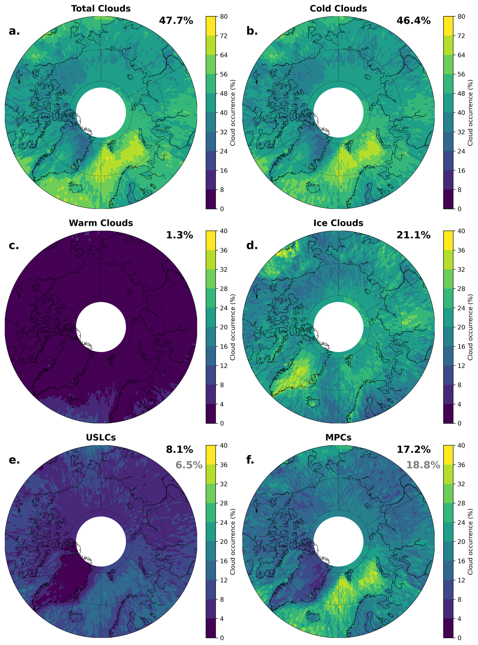
Figure 3 Stereographic projections of the occurrence of low-level (between the clutter height and 3 km a.g.l.) cloud types between 2007 and 2016: (a) total clouds, (b) cold clouds, (c) warm clouds, (d) ice clouds, (e) USLCs, and (f) MPCs. The black numbers shown in the upper right of each subfigure are relative to the median occurrence over the entire study area. The gray numbers indicate the median occurrence of clouds whose phase classification may be affected by radar clutter.

Based on the spatial distribution of the cloud-type occurrence, on the main weather patterns (high- and low-pressure systems) and geographical limits (latitudes, oceans, continents), we choose to subdivide the Arctic into 12 distinct subregions (Fig. 4a). The six subregions in Zone 1 have latitudes ranging from 60 to 70° N, whereas the northernmost regions are located within the high-latitude ring, which extends from 70 to 82° N (Zone 2). Subregions 1B and 2B, as well as 1C and 2C, are merged to increase the statistical significance of the results (1-2B and 1-2C). The purpose of this regionalization is to highlight the specific features of the low-level cloud occurrence in the Arctic. A statistical analysis of total cloud occurrences for each region is presented in Fig. S8 and discussed in Sect. S2 of the Supplement.

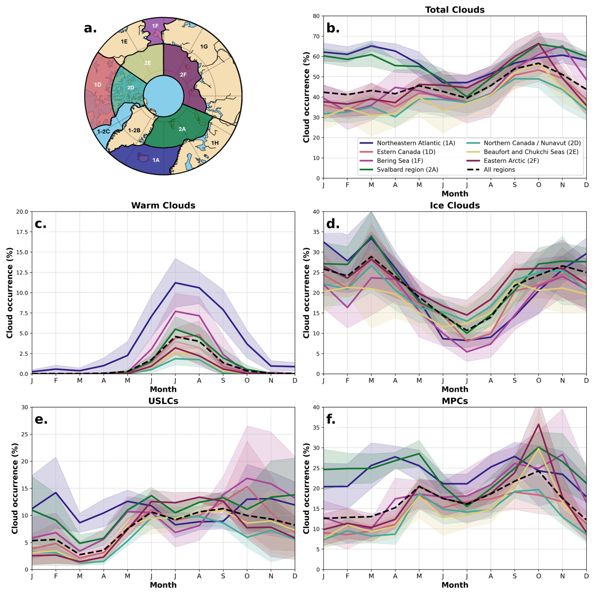
Figure 4 Monthly occurrence variations for different types of low-level clouds (between the clutter height and 3 km a.g.l.) between 2007 and 2016: (b) total clouds, (c) warm clouds, (d) ice clouds, (e) USLCs, and (f) MPCs. Regionalization (a) with colored regions for monthly analysis. The colored areas around the curves represent the interquartile range. Zone 1 represents the low-latitude regions from 60 to 70° N, excluding the Russian continental region. The letters for the different regions start from the North Atlantic zone (1A) and run from west to east. Zone 2 is the second high-latitude ring, from 70 to 82° N. Regions in this latitude band are referred to in the same way as the first ring.

The northeast Atlantic sector (region 1A) is the area with the highest occurrence of warm clouds (≈ 5 %–10 %). MPCs are also frequent in this region, as well as over the seas surrounding the Svalbard Archipelago (region 2A), where they occur up to 35 % of the time. These two regions are influenced by the Gulf Stream and low-pressure systems. They are characterized by the highest low-level cloud occurrence (OC_all-ll > 60 %). A specific feature of region 2A is the prevalence of MPCs and USCLs over the Greenland, Barents, and Norwegian Seas (OC_USLCs with peaks around 20 %). Low-level ice clouds are more prevalent in mountainous regions of Alaska, Greenland, and western Canada (1E) (OC_ice > 25 %) than in eastern provinces of Canada (1D) and, to a lesser extent, than in the Labrador Sea and Baffin Bay (1-2C). In these latter regions and parts of eastern Europe (1H), USLCs occur more frequently than in continental areas with relief of western Canada (1E) and central and eastern Russia (1G), for which OC_USLCs is lower than 10 %. The cloud-type cover over the Bering Sea sector (1F) differs from that in neighboring regions. The frequency of occurrence of low-level clouds and of liquid-containing clouds in particular is much higher (OC_MPCs≈25 % and OC_USLCs > 10 %) than in surrounding regions subject to high-pressure systems. The northernmost eastern sector of the Arctic (2F) is more cloudy (OC_all-ll≈50 %) than the Beaufort and Chukchi Seas (2E) and the northern Nunavut region of Canada (2D). Region 2E experiences a 5 % higher occurrence of MPCs than region 2D. In summary, these first results show that the distribution of low-level ice clouds and liquid-containing clouds is characterized by strong regional contrasts partly influenced by the latitude-driven air temperature and the type of surface (ocean, sea ice, continental relief).

3.2 Seasonal variability of low-level cloud occurrences

In this section, we investigate the seasonal variations of low-level cloudiness (between the clutter height and 3 km a.g.l.) for seven contrasting subregions of the Arctic. The results are presented in Fig. 4. It shows that in most regions, the annual cycle of total low-level cloud occurrence exhibits two distinct seasonal maxima. The first peak occurs in late spring, when low-level clouds are present 45 % of the time in the Arctic (Fig. 4b, dashed black line). Previous studies have highlighted that the first cloud maximum is related to changes in the regional atmospheric circulation resulting from the weakening of the tropospheric polar vortex at the end of winter (Kay and Gettelman, 2009; Morrison et al., 2018). The second peak has a larger amplitude, reaching 55 % in autumn. However, the magnitude and timing of this double seasonal peak of high cloudiness exhibit regional variability. Most of the regions north of 70° N (2D, 2E, and 2F) are characterized by well-marked peaks with above average low-level cloud occurrences in May and in October or November. This feature is particularly striking in the eastern Arctic region (2F), where low-level cloud occurrence reaches almost 45 % in May and 68 % in October. Over the Bering Sea (1F), the spring and autumn local maxima are also clearly defined but more likely occur in April and November. This pronounced seasonal variation is less evident in regions influenced by the Atlantic Ocean (1A and 2A). Typically, higher and steadier occurrences are observed throughout the year (from 48 % to 65 % in region 1A). The second peak of cloud occurrence observed in the autumn can be attributed to changes in surface conditions. In the northern regions (2E and 2F), sea ice retreat peaks in September. The open ocean facilitates the vertical transfer of moisture to the atmosphere, which promotes the development of low-level clouds until the return of the ice pack (Stroeve et al., 2012; Morrison et al., 2019; Yu et al., 2019).

The seasonal cycle of warm liquid clouds and ice clouds does not exhibit the two seasonal maxima observed for total low-level clouds. As expected, the occurrence of low-level warm clouds is characterized by a single seasonal maximum, occurring in summer (Fig. 4c). The pan-Arctic median OC_warm reaches 5 % in July. These clouds are mainly observed in low-latitude Arctic regions (1A, 1D, and 1F), where a maximum frequency of occurrence of 11 % is recorded over the Northeast Atlantic region (1A) in July. Region 1A is also the only sector to experience warm cloud cover from mid-autumn to late spring. The monthly variations of low-level ice clouds are opposite to those of warm clouds. The occurrence of ice clouds is at its maximum in all regions from mid-autumn to late winter (Fig. 4d). During this period, OC_ice ranges from 20 % to 30 %. In the southern Arctic (1A, 1D, and 1F), the amount of ice clouds decreases considerably in spring, dropping to a minimum value of below 10 % in summer. However, this decrease is less steep over the northern seas of the western (2D and 2E) and eastern (2F) Arctic, where the persistence of low-level ice clouds is favored by the colder atmospheric conditions. In these regions, OC_ice is typically greater than 10 % even during the summer months.

At the scale of the Arctic, the temporal evolution of the frequency of occurrence of USLCs (OC_USLCs) and MPCs (OC_MPCs) is similar to that of total clouds. Figure 4e and f show a seasonal cycle featuring two peaks. The late spring peak is just over 10 % for USLCs and over 20 % for MPCs. The second peak occurs in September for USLCs and in October for MPCs, reaching more than 10 % and 25 %, respectively. The secondary seasonal peak is also broader for USLCs than for MPCs. Significant differences are observed when these seasonal patterns are investigated at a regional scale. In autumn, when the second peak occurs, OC_MPCs reaches 35 % over the seas north of Siberia (2F). Differences in OC_MPCs of almost 15 % are also observed in spring between the Northeastern Atlantic region (1A) and region 1F. Moreover, regions 2F and 2E shift from being amongst the least covered by MPCs in summer (less than 20 % and 15 %, respectively) to becoming the regions with the highest MPCs occurrence in mid-fall (OC_MPCs is 30 % to 35 %). In these regions, the opposite trend is observed for USLCs, with relatively high and steady values of OC_USLCs observed in summer, followed by a sharp decrease in autumn. Regions influenced by the transport of heat and moisture from the Atlantic Ocean (1A and 2A) exhibit the highest occurrences of MPCs during winter and spring (up to 25 % in region 1A). In contrast, the western and eastern Arctic regions (1F, 2D, 2E, and 2F) have lower than average MPCs occurrence values (8 %–10 %). These regional differences also exist for USLCs but remain less pronounced. Interestingly, the significant reduction of OC_USLCs observed at the beginning of spring (March) in the marine regions 1A, 2A, and 1F is balanced by an increase in ice clouds and a more moderate one in MPCs. From a broader perspective, the regional variations in the seasonal occurrence of these liquid-containing clouds cannot be explained solely by latitudinal temperature gradients and surface conditions. The frequency of occurrence of these clouds appears to be controlled by several environmental factors. Furthermore, our results show that USLCs and MPCs have a contrasted seasonal distribution at a regional scale, supporting the relevance of studying these clouds separately.

3.3 Linking cloud-type occurrence to environmental conditions

3.3.1 Regional environmental conditions

In this section, the influence of environmental conditions on the regional and seasonal occurrence of low-level warm liquid clouds, ice clouds, USLCs, and MPCs is investigated. Multiple linear regression (MLR) analyses are implemented to study the impact of the selected set of parameters (Sect. 2) on the distribution of cloud-type occurrences. Figures 5 and 6 show the normalized MLR coefficients for the four types of low-level clouds in four Arctic regions (1A, 1D, 2A, and 2F) during the different seasons. These four regions were selected on the basis of their distinct seasonal variability, surface conditions (oceanic, continental, and sea ice), and geographical location as described in Sect. 3.2. The MLR analysis shows that three parameters explain most of the variability in cloud occurrences. Surface temperature is anti-correlated with OC_ice and positively correlated with OC_warm and OC_USLCs (except during summer for USLCs). The impact of LTS generally follows the same trend as the surface temperature, highlighting more stable conditions associated with larger liquid cloud occurrences. The specific humidity at 700 hPa is positively correlated with OC_ice and negatively correlated with OC_USLCs. SH_700hPa is also anticorrelated with OC_warm, except in autumn over high-latitude regions, where a weak positive correlation is observed.

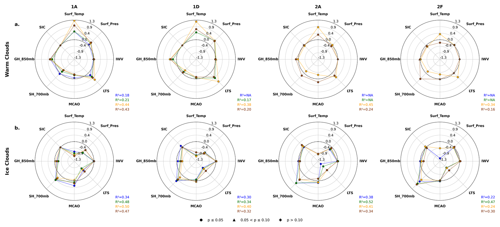
Figure 5 Normalized coefficients of MLR for low-level (a) warm clouds and (b) ice clouds for 4 regions (1A, 1D, 2A, and 2F) during the 4 seasons: (blue) winter, (green) spring, (orange) summer, and (brown) autumn. The statistical significance of each coefficient is represented by symbols: circles are associated with p-values ≤ 0.05, triangles with 0.05 < p-values ≤ 0.10, and crosses with p-values > 0.10. The dashed black line corresponds to normalized coefficients equal to zero. Only MLR results with a coefficient of determination R² > 0.10 are displayed.

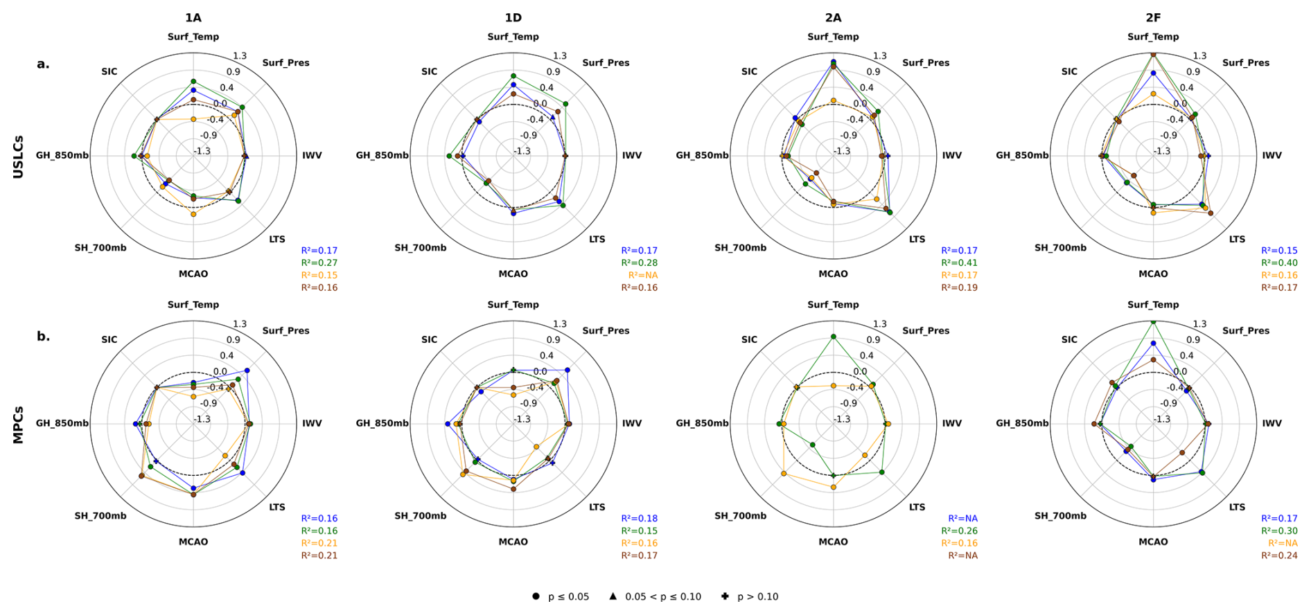
Figure 6 Normalized coefficients of MLR for low-level (a) USLCs and (b) MPCs for 4 regions (1A, 1D, 2A, and 2F) during the 4 seasons: (blue) winter, (green) spring, (orange) summer, and (brown) autumn. The statistical significance of each coefficient is represented by symbols: circles are associated with p-values ≤ 0.05, triangles with 0.05 < p-values ≤ 0.10, and crosses with p-values > 0.10. The dashed black line corresponds to normalized coefficients equal to zero. Only MLR results with a coefficient of determination R² > 0.10 are displayed.

Figure 5a confirms that an increased occurrence of warm liquid clouds is primarily associated with warmer surface temperatures and more stable conditions, which are likely related to stronger inversions. The correlations are stronger in summer, especially in lower-latitude regions (regions 1A and 1D, R² > 0.4). In the North Atlantic region, the results of the MLR also show that negative SH_700hPa coefficients (i.e., anticorrelation) are associated with positive LTS coefficients in summer and to a lesser extent in autumn. This indicates that the maintenance of warm liquid clouds is also facilitated by the supply of heat and moisture from the surface, as previously shown by Morrison et al. (2019) and Taylor and Monroe (2023). Anticorrelations between OC_warm and the MCAO index (negative MCAO values) are observed during summer in all selected marine regions. This confirms that warm air intrusions also contribute to the persistence of low-level warm clouds. This is particularly true in the Northeastern Atlantic sector (1A) and in the Svalbard region (2A), where southerly intrusions of warm and moist air appear to influence cloud occurrence in all seasons, as previously reported by Woods and Caballero (2016).

Low-level ice clouds are observed more frequently in cold, humid, and less stable atmospheric conditions, regardless of the season (Fig. 5b). The MLR analysis shows that the occurrence of ice clouds is associated not only with lower temperature and LTS but also with higher specific humidity at 700 hPa. This indicates that moist conditions in the lower free troposphere near the top of low-level clouds can promote the formation of ice crystals within this cloud layer. In all regions, anticorrelations between OC_ice and geopotential heights at 850 hPa (GH_850hPa) suggest that ice clouds are observed more frequently in low-pressure systems, particularly in spring. It is also interesting to note that variations in sea ice concentration (SIC) do not appear to play a significant role in the occurrence of ice clouds, except in the Svalbard region (2A) during autumn.

The variability of the USLCs cloud cover is mainly influenced by changes in temperature, humidity, and stability conditions. However, Fig. 6a shows that the trends are opposite to those of ice clouds. From autumn to late spring, more stable atmospheric conditions associated with higher temperatures and humidity confined to the lower layers favor the persistence of unglaciated supercooled liquid clouds. These relationships are particularly strong in regions 2F and 2A, and differ significantly from those established for ice and warm clouds. Our results also suggest that summer USLCs occur more frequently when the regions are exposed to cold air mass intrusions (positive MCAO and lower air temperature), which contrasts with the pattern observed for warm clouds.

Interpreting MLR results for MPCs is more challenging, as their seasonal and regional patterns exhibit substantial variability. This reflects the complex nature of mixed-phase clouds, which result from a combination of thermodynamic, dynamical, radiative, and surface-related processes that can vary significantly between seasons and regions. Figure 6b shows that the presence of MPCs over marine regions (1A and 2A during summer) is linked to an increase of cold air outbreaks and moisture intrusions (especially in spring and summer). In the Svalbard region (2A), MPCs are frequent throughout the year. Our results indicate that their increased occurrence during summer is associated with colder atmospheric conditions linked to intrusions of cold, moist air, as suggested by positive correlations with MCAO and SH_700hPa. In contrast, higher MPCs occurrence appears to be favored by warmer air masses and enhanced lower-tropospheric stability in region 2A during spring and throughout most seasons in region 2E.

Overall, the results highlight differences between USLCs and MPCs that are primarily linked to the presence of the ice phase. The increase of OC_USLCs is generally associated with warmer and more stable conditions, in which the clouds predominantly remain in the liquid phase. Higher OC_MPCs are observed under colder conditions, where the formation of the ice phase within the cloud layer is promoted. Although both cloud types can form in similar large-scale thermodynamical regimes, our MLR results show that they have different statistical relationships with temperature, humidity, and stability. In particular, at lower latitudes, higher MPC occurrences are more likely statistically associated with colder atmospheric conditions, enhanced specific humidity at 700 hPa, and positive MCAO values, which are indicative of more unstable lower-tropospheric potential temperature profiles.

3.3.2 Key environmental factors controlling the cloud-type distribution

The purpose of this section is to investigate the variability of the dominant environmental parameters that drive the low-level cloudiness (between clutter height and 3 km a.g.l.) at both the regional and intra-regional scales. Regressions are performed for each grid point (1° latitude by 1° longitude), season, and cloud type, but only the most influential MLR coefficient with R² > 0.1 is selected, in line with previous studies of Naud et al. (2023) and Scott et al. (2020). Figure 7 confirms that on an annual basis, surface temperature, MCAO, LTS, geopotential height, and specific humidity are the main drivers of the variability in low-level cloud occurrences. However, intra-regional differences emerge when the most influential parameters are examined at a more local scale.

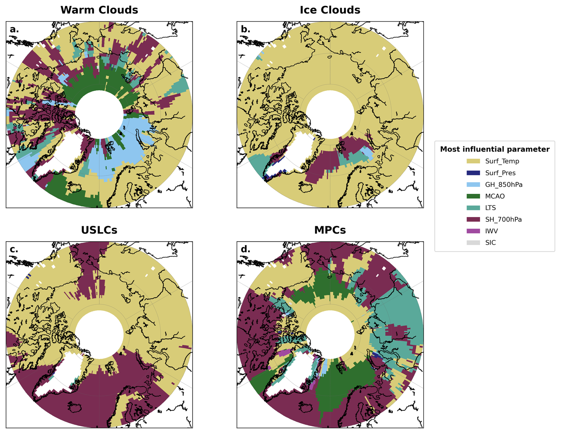
Figure 7 Most influential parameters of MLR for low-level (a) warm clouds, (b) ice clouds, (c) USLCs, and (d) MPCs for all seasons. Empty grid cells indicate regions where the MLR yields an R² < 0.1 or where one or more required thermodynamic parameters are missing.

Figure 7a shows that GH_850hPa is the dominant factor controlling the frequency of occurrence of low-level warm clouds in regions influenced by the North Atlantic Ocean. The advection of warm air masses is typically associated with higher geopotential heights, which favor the formation of liquid clouds. In high-latitude marine regions, MCAO also emerges as a major controlling parameter. During periods of reduced sea ice extent, these areas appear especially sensitive to intrusions of relatively warm and moist air masses, which promote the persistence of the liquid phase. Elsewhere, the spatial distribution of warm-cloud occurrence is mainly driven by surface air temperature, except in some continental regions where SH_700hPa and LTS dominate the warm cloud patterns.

In most of the eastern and western Arctic regions (Canada or Russia), surface air temperature is the dominant factor controlling the occurrence of low-level ice clouds (negative correlation, Fig. 7b) and USLCs (positive correlation, Fig. 7c). However, in lower latitude maritime regions (Bering Sea, Atlantic Ocean, and seas in the vicinity of Greenland, Svalbard and part of Alaska), specific humidity at 700 hPa is the primary factor explaining the regional distribution of USLCs (negative correlation). Geopotential height at 850 hPa and LTS (negative correlations) may also be significant contributors to the ice-cloud variability in the seas close to Greenland and Svalbard.

Figure 7d shows that the dominant factor controlling the distribution of MPCs occurrence varies significantly across the regions. On an annual average, marine regions where the fraction of MPCs is high (1A, 2A, Beaufort, and Chukchi seas) are mostly influenced by MCAO. The impact of cold-air outbreaks on MPCs is stronger during the transitional seasons (spring and autumn), whereas the advection of warm air and moisture above the oceans sustains the liquid phase of warm clouds in summer and of USLCs in spring (Fig. S9 in the Supplement). In central Russia, LTS is the dominant MPCs controlling factor (positive correlation), whereas surface temperature and specific humidity at 700 hPa are the most influential parameters in eastern and western arctic regions.

More generally, our results highlight significant regional contrasts in the distribution of the cloud phase, which are primarily associated with large-scale variations in temperature and moisture advection. In southern latitude marine regions, parameters related to air mass intrusions (MCAO) and to the thermodynamic properties of the lower troposphere, such as SH_700hPa, are found to play a dominant role in shaping the phase partitioning of low-level cold clouds (MPCs, ice clouds, and USLCs). Over continental regions, the distribution of cloud phases is more frequently associated with lower-tropospheric stability (LTS) and with colder thermodynamic conditions aloft, which are statistically linked to an enhanced occurrence of the ice phase. These first-order interpretations show that it is necessary to study in greater detail the links between the regional cloud characteristics and the surface conditions. The surface properties directly influence the stability of the lower atmospheric layers, the strength of the temperature and moisture inversions (Brooks et al., 2017), which in turn impact the efficiency of turbulent fluxes and vertical mixing with the cloud layers. In the absence of reliable data on vertical velocities and surface fluxes, a statistical analysis of the fraction of clouds coupled to the surface across different seasons and regions can provide insight into these turbulent-driven processes.

3.3.3 Cloud–surface coupling

This section aims to characterize the coupling between low-level clouds and the surface by analyzing the fraction of clouds that are thermodynamically coupled to the surface. Low-level clouds are defined here as clouds located between the upper limit of the radar clutter region and 3 km (a.g.l.). The analysis focuses on how the fraction of coupled clouds varies as a function of surface type (open water, sea ice, and land) and cloud type, thus providing insight into the role of underlying surface properties in modulating cloud–surface interactions.

Figure 8 (a) Stereographic projection of median coupled low-level (between clutter height and 3 km a.g.l.) cloud fractions for the period 2007–2016. The number in the upper left indicates the median fraction for the entire study area. (b) Monthly evolution of the fraction of surface-coupled low-level clouds for all surface types combined (black) and separately for open ocean (blue), land (brown), and sea ice (gray). Percentages indicated at the top of the panel correspond to the annual median coupled-cloud fraction for each surface category, using the same color code. (c) Monthly evolution of coupled low-level cloud fractions over 2007–2016. Shaded areas around the curves represent the interquartile range.

Figure 8a shows a stereographic map of the average annual spatial distribution of coupled clouds, expressed as a proportion of the total number of low-level clouds (fraction). On average, nearly 17 % of low-level clouds in the Arctic are coupled with the surface. A higher proportion of coupled clouds are observed in oceanic regions (1A, 1-2C, 2A, and 1F), such as the Greenland, Norwegian, and Barentz Seas surrounding Svalbard. There, the annual average fraction exceeds 40 %, which contrasts with those obtained in the continental regions of Greenland, western Canada, central and eastern Russia, where fractions of less than 15 % are usually found. Figure 8b shows the monthly evolution of the fraction of surface-coupled low-level clouds over open water, land, and sea ice. Coupled clouds are consistently more frequent over open ocean and seas throughout the year, with monthly fractions generally exceeding those over land and sea ice. In marine regions, the coupled-cloud fraction typically ranges from approximately 30 % to 40 %, with pronounced minima observed during summer (< 15 %). In contrast, significantly lower values are observed over land and sea ice, with median coupled-cloud fractions of approximately 10 % and 12 %, respectively.

Figure 8c shows the monthly evolution of the coupled cloud fractions over the selected regions defined in Fig. 4a. It confirms that clouds are more frequently coupled to the surface in maritime regions influenced by the North Atlantic (1A and 2A) and Pacific oceans (1F). From mid-autumn to mid-spring, the fraction of coupled clouds falls within the range of 30 % to 40 %. A pronounced autumn peak is observed in the Bering Sea and Svalbard regions, indicating that more than 35 % of the low-level clouds are coupled to the surface. A less substantial but still noticeable maximum also appears in most of the northern seas (2E and 2F, peaking at 27 % to 35 % in October) and some continental regions (1D and 2D, with autumn maxima close to 20 %). Another local maximum ranging from 18 % to 25 % can be observed in April or May in all regions except marine regions (1A and 2A). In winter, minimum fractions of coupled clouds are observed in mostly continental and sea ice regions (less than 10 %). In marine regions (1A, 1F, and 2A), the fraction of coupled clouds remains above 30 % during winter, reaching values of up to 40 % across the seas surrounding the Svalbard archipelago. Our results also indicate that low-level clouds are mainly decoupled from the surface in summer in all regions (coupled fraction ranging from 20 % in 1A down to 8 % in 2E).

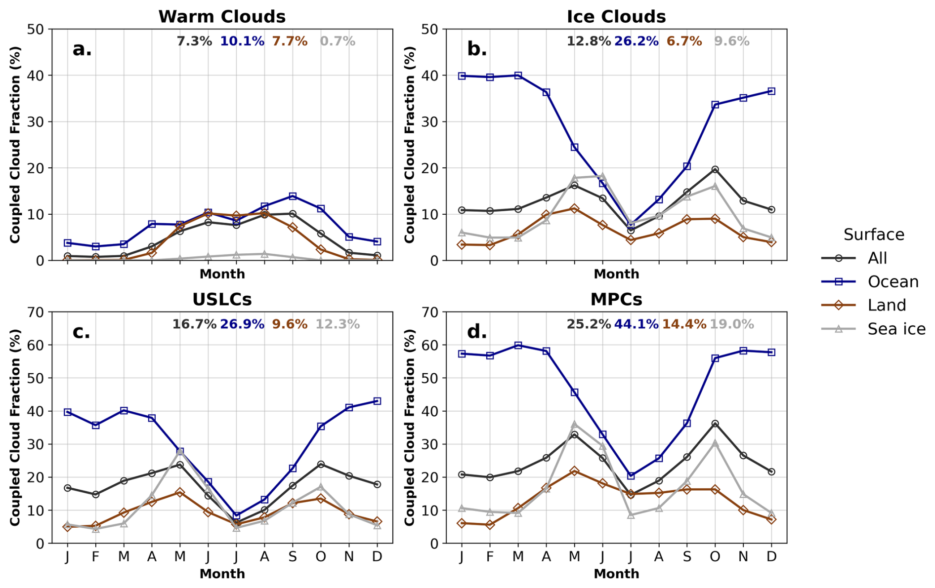
Figure 9 Monthly evolution of low-level (between clutter height and 3 km a.g.l.) coupled cloud fractions over different surface types (ocean, land, sea ice, and all surfaces). Panels show (a) warm clouds, (b) ice clouds, (c) USLCs, and (d) MPCs.

However, these results are only representative of clouds located between the clutter height and 3 km (a.g.l.), regardless of their thermodynamic phase. Figure 9 depicts the seasonal evolution of the coupled cloud fractions of the four different cloud types over open ocean, land, and sea-ice surfaces. Significant seasonal differences emerge between warm clouds and ice clouds that were not captured when the surface coupling was investigated at a regional scale. The results show that the majority of warm clouds are decoupled from the surface. The highest fraction of coupled clouds is found at the end of summer over oceans (12 % in September; Fig. 9a). The pattern for low-level ice clouds is the opposite (Fig. 9b). From October to April, maximum values of 30 %–40 % are observed for the fraction of coupled clouds above open seas. During this period, the average cloud top height is close to 2200 m, which is more than twice that observed for low-level warm clouds coupled to the open ocean (Fig. S10a in the Supplement). In summer, a minimum proportion of coupled ice clouds is observed (8 % in July), when these clouds are typically found at higher altitudes. Over land and sea ice, the seasonal cycle is characterized by two maxima occurring in May and October. For sea ice, the coupled-cloud fraction reaches values close to 15 %, while slightly lower maxima of about 10 % are found over continental surfaces. Outside these periods, the fraction of coupled ice clouds remains generally low over land and sea ice. Interestingly, our results also show that the average cloud top height of ice clouds coupled with sea ice surface is close to 2500 m, which is higher than over open sea (Fig. S10b).

USLCs and MPCs share similar monthly variations, characterized by two maxima in May and October when investigated regardless of the surface type (black curves; Fig. 9c–d). However, these maxima are more pronounced for MPCs. The coupled-cloud fraction reaches 30 %–35 %, compared to values below 25 % for USLCs. A summer minimum is also observed, with values of about 15 % for MPCs and below 10 % for USLCs. These differences become even more marked over the ocean, where from October to May approximately 60 % of MPCs are coupled to the surface (Fig. 9d), compared to about 40 % for USLCs (Fig. 9c). Annual median values further emphasize this contrast, with 44 % of MPCs coupled over open water, compared to only 19 % over sea ice. Interestingly, MPCs are more frequently coupled than USLCs over oceanic surfaces, despite having higher cloud-top heights (approximately 1800 m for MPCs and 1200 m for USLCs; Fig. S10c–d), suggesting that cloud–surface coupling is not solely controlled by cloud-top proximity to the surface.

Overall, our results indicate that the highest fraction of coupled cold clouds is usually above open water when strong temperature gradients occur between the surface and the lower troposphere (winter, spring, and autumn). However, the seasonal cycle of coupled clouds varies significantly with the cloud type (ice, mixed, and supercooled liquid) and the surface conditions. In the following section, we will discuss how these surface processes, in combination with larger-scale thermodynamic conditions, affect the occurrence of MPCs and USLCs.

4 Discussion

In this section, we discuss our results in the context of previous ground- and satellite-based studies, as well as the thermodynamic conditions favorable to the persistence of the different types of low-level clouds. Figure 10 compares the seasonal distribution of the frequency of occurrence of low-level and tropospheric column clouds (total clouds) to previous measurements conducted at specific sites or regions in the Arctic. The seasonal variability of low-level clouds, as inferred from our analysis, compares well with previous results derived from satellite observations across the Pan-Arctic (Philipp et al., 2020), the main marine regions of the Arctic (Jiang et al., 2024), and more locally over Barrow (Zhao and Wang, 2010). From autumn to early spring, we observe approximately 10 % higher occurrences in the marine regions of the European Arctic than that reported by Jiang et al. (2024), based on 14 years of CALIPSO-GOCCP lidar observations. However, DARDAR-SOCP occurrence values are similar to the latter observations in the marine regions of the eastern and western Arctic. The absolute deviation of the occurrence between the two datasets is usually less than 5 %, except in March and May, when it can reach 10 %. Figure 10b also shows that previous estimates based on AVHRR passive remote sensing measurements (Philipp et al., 2020) are significantly lower (by up to 20 %) than those obtained in our study, especially from late autumn to early spring. Passive remote sensing may underestimate low-level cloud fraction due to the low contrast between clouds and the underlying surface (Chan and Comiso, 2013).

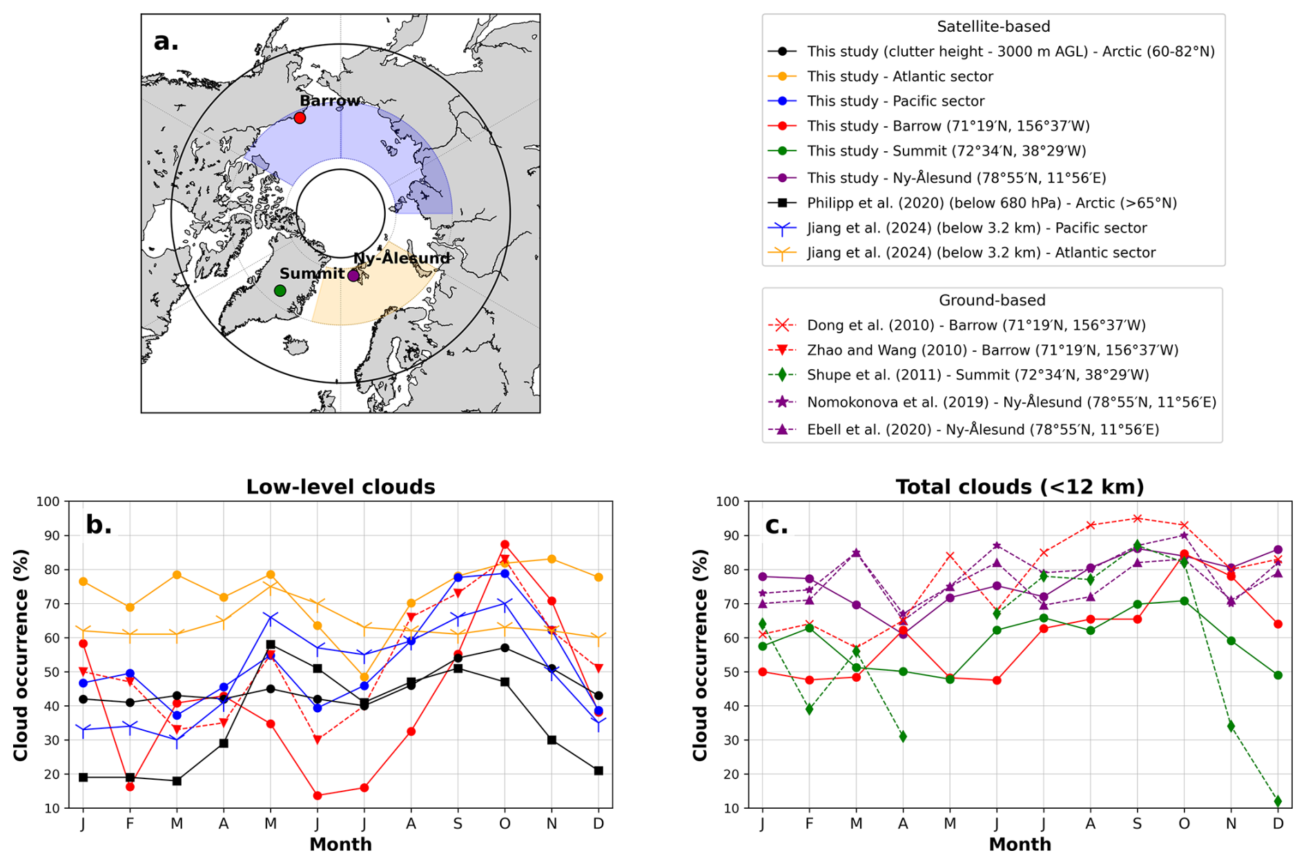
Figure 10 Monthly cloud occurrence in the Arctic derived from satellite observations and compared with previous satellite- and ground-based studies. Panel (a) represents the map of the Arctic study domain used in this work. The black circle outlines the Arctic region between 60 and 82° N, which defines the spatial domain considered in this study. The shaded sectors indicate the regions used for these comparisons: the Arctic Pacific (blue shading) and the Arctic Atlantic sector (orange shading). Colored dots indicate the locations of the ground-based sites: Barrow (red; 71°19^′ N, 156°37^′ W), Summit (green; 72°34^′ N, 38°29^′ W), and Ny-Ålesund (purple; 78°55^′ N, 11°56^′ E). Panel (b) represents the monthly occurrence of low-level clouds, while panel (c) represents the monthly occurrence of total clouds below 12 km. The line styles and symbols represent the different studies, as indicated in the legend, including satellite-based estimates (Philipp et al., 2020; Jiang et al., 2024) and ground-based observations (Dong et al., 2010; Zhao and Wang, 2010; Shupe et al., 2011; Nomokonova et al., 2019; Ebell et al., 2020).

Interestingly, our estimates of low-level cloud occurrence are in fairly good agreement with the ground-based observations reported by Zhao and Wang (2010) in Barrow, despite differences of up to 15 % from late summer to winter. In our analyses, clouds located between the ground and the clutter are not accounted for, unlike in ground-based observations. This could explain why DARDAR-SOCP cloud occurrence retrievals are underestimated during these seasons, when clouds are frequent in the lowest layers of the troposphere.

Previous results on the occurrence of pan-Arctic low-level clouds are scarce despite their importance for the surface energy budget. Most studies have instead focused on the analysis of the occurrence of Arctic clouds throughout the tropospheric column. Mioche et al. (2015) and Cesana et al. (2024) used four years of DARDAR-MASK products (with different versions and resolutions) to show that tropospheric clouds were detected on average more than 70 % and 77 % of the time, respectively. Matus and L'Ecuyer (2017) analyzed four years of 2B-CLDCLASS-LIDAR cloud phase classification products to obtain an annual cloud occurrence of nearly 75 %. Across the entire tropospheric column, we obtain an eight-year average cloud occurrence close to 65 %, which is consistent with these previous estimates. Figure 10c displays more spatially resolved comparisons with ground based measurements at three sites (Ny-Ålesund, Barrow, and Summit). The cloud seasonal distribution and the occurrence values derived from DARDAR-SOCP agree with the ground-based data from Ny-Ålesund (Nomokonova et al., 2019; Ebell et al., 2020). Differences in occurrences are usually less than 5 %–10 %. Higher discrepancies can be observed over Barrow and Summit stations. While the cloud seasonal variations are generally in accordance between the datasets, our retrievals underestimate the occurrence of clouds compared to ground-based observations reported in Dong et al. (2010) and Shupe et al. (2011). Differences of up to 20 % are observed from May to September over Barrow and more than 10 %–15 % over Summit from late August to the end of winter. The wider clutter zone coupled with the presence of thin clouds close to the surface could explain part of the discrepancies (Marchand et al., 2008). Overall, these comparisons with previous active remote sensing observations and products support the significance of our results, which were obtained using DARDAR-MASK v2.23 with the DARDAR-SOCP algorithm.

In most regions of the western and eastern Arctic, our results showed that low-level cloud occurrence exhibits a seasonal cycle characterized by two maxima, occurring in spring and autumn. The first seasonal peak can be attributed to changes in weather conditions (e.g., cyclonic flows, warm air advections, etc.) that occur at the end of winter (Yu et al., 2019). The high cloud cover observed in autumn is probably a consequence of the changing surface conditions as suggested by Taylor and Monroe (2023) and Cesana et al. (2024). During this season, the minimum extent of the sea ice facilitates the supply of moisture from the surface. Our results indicate that this seasonal pattern is more pronounced in northern regions of the eastern Arctic and over the Beaufort Sea. In these regions, the slower retreat of the sea ice compared to other areas affects the timing of the second seasonal peak (Yu et al., 2019). The study of Jiang et al. (2024) also suggested a similar regional specificity for low-level cloud cover in autumn.

Our results show that areas influenced by the North Atlantic Ocean are the cloudiest regions in the Arctic throughout the year. This finding is consistent with previous studies by Mioche et al. (2015) and Jiang et al. (2024). In the Northeast Atlantic sector and across the seas near the Svalbard archipelago, we find annual low-level cloud occurrences of 56 % and nearly 60 %, respectively. In contrast, the annual mean occurrence over the Russian Arctic is much lower, reaching only 37 %. These land–ocean contrasts are more pronounced in winter over these regions. This could be due to differences in the large-scale transport of heat and moisture, with warm air intrusions (WAI) occurring more frequently and more intensely over the Atlantic sector than in continental regions (Woods and Caballero, 2016; Johansson et al., 2017; Nygård et al., 2019). While WAI can be associated with an increase in cloudiness, cold air outbreaks (CAO) and thermal contrasts between the surface and the lower troposphere can also affect the geographical and seasonal distribution of low-level clouds (Fletcher et al., 2016; Gierens et al., 2020). Over open oceans, stronger surface turbulent fluxes facilitate vertical transfer of heat and moisture. This, in turn, promotes the formation, coupling, and persistence of low-level clouds (as discussed in Wendisch et al., 2023b).

At the pan-Arctic scale, our results show that approximately 17 % of low-level clouds are coupled to the surface. When restricting our analysis to a period comparable to that of the ASCOS campaign (Tjernström et al., 2014) and to a similar geographical domain (limited to 82° N in our case), we find that the fractions of coupled total low-level clouds and MPCs are approximately 15 % and 17 %, respectively. These values are consistent with the 23 % reported during ASCOS (Sotiropoulou et al., 2014), despite differences in the sampling strategy and cloud detection methods employed. In particular, a substantial fraction of the low-level clouds obtained from our dataset is located below 500 m. This altitude range can be strongly affected by radar clutter and surface contamination, thus leading to an underestimation of the fraction of coupled clouds. We show that the spatial distribution of coupled clouds exhibits pronounced contrasts. Higher fractions of coupled clouds are observed over the open water of the Atlantic and Pacific sectors than over continental and sea ice regions. From late autumn to mid-spring, this fraction exceeds 50 % in the seas surrounding Svalbard, which is slightly lower than the value of 60 % reported by Griesche et al. (2021).

One interesting aspect of our study concerns the regional and seasonal variability of the cloud phase. Our results show that warm and ice clouds exhibit opposite seasonal cycles. This is consistent with the study of Yu et al. (2019), who reported a comparable seasonal evolution of monthly mean liquid and ice water paths for Arctic low-level clouds. Warm clouds are mostly decoupled from the surface. These clouds are promoted by advection of warm air. Our results suggest that they evolve toward greater coupling with the surface during summer (in line with Morrison et al., 2012, and Brooks et al., 2017). From mid-autumn to early spring, low-level ice clouds prevail over other cloud types across all regions. Our analysis indicates that the ice cloud occurrence is favored by low temperatures, high moisture availability, and enhanced atmospheric dynamical activity. These atmospheric conditions are frequently encountered within cyclonic regimes, which is consistent with previous findings of Liu et al. (2017).

Only a few studies have estimated the regional and seasonal occurrence of low-level MPCs, and to our knowledge, no studies have targeted Arctic USLCs specifically. Together, these cold liquid-containing clouds account for nearly 60 % of low-level clouds. This finding aligns with the results of Cesana et al. (2012), obtained from four years of CALIOP lidar observations. However, our findings show a higher median occurrence of low-level MPCs than the earlier CloudSat-CALIPSO-based estimates of Matus and L'Ecuyer (2017) (i.e., 15 % throughout the entire tropospheric column). Unlike this study, we do not limit MPCs to single mixed-phase layers. Instead, we also include combinations of several successive liquid, mixed, and/or ice layers in our definition of MPCs. We believe that this representation more accurately reflects in situ observations, showing that low-level MPCs frequently consist of stratiform layers of supercooled droplets near the cloud top, as well as mixed-phase and ice layers below (McFarquhar et al., 2007; Mioche et al., 2015).

Our analyses show that the occurrence of liquid-containing clouds (MPCs and USLCs) follows a pronounced seasonal cycle. Maxima are observed during the transitional seasons of spring and autumn, confirming previous findings of Jiang et al. (2024). Across the Svalbard region, our results on MPCs occurrence and seasonal variability are consistent with previous estimates based on CloudSat-CALIPSO observations (Mioche et al., 2015). Interestingly, USLCs occur more frequently when the lower atmosphere is more stable and surface pressures are higher. Our results also show that, above open water, USLCs have lower heights and are less frequently coupled to the surface than MPCs, especially in winter and spring. This result is consistent with earlier findings showing that ice-containing clouds are more often dynamically coupled to the boundary layer (Griesche et al., 2021). This could be a consequence of large-scale subsidence events, which would lead to stronger temperature inversions and more efficient mixing in the shallower marine boundary layer (Myers and Norris, 2013). Young et al. (2018) further investigated the impact of large-scale subsidence on the development of convection and the microphysical properties of marine stratiform, liquid-containing clouds. Their simulations showed that large-scale subsidence tends to reduce the entrainment of air from above into the cloud while increasing the cloud's liquid water path, the cloud-top radiative cooling, and downdrafts. The resulting vertical mixing (and coupling) would help sustain the liquid phase and prevent rapid glaciation of the cloud.

Over continental and sea ice regions, the contrasting behavior of MPCs and USLCs appears to be primarily linked to differences in the thermodynamic structure of the lower atmosphere and to the processes controlling the initiation of the ice phase. While both cloud types are influenced by surface air temperature and lower-tropospheric stability, USLCs are preferentially associated with a more stable boundary layer and a reduced moisture availability above cloud top (here characterized at 700 hPa). The partitioning between MPCs and USLCs appears particularly sensitive to moisture conditions near cloud top, which can modulate the onset of the ice phase. At the regional scale, mixed-phase clouds are generally less frequent over land and sea ice than over the open ocean, consistent with a reduced surface moisture supply. However, during periods of stronger surface–atmosphere exchange – such as autumn in marginal sea ice zones or during large-scale advection events – conditions become more favorable for sustaining the ice phase, in agreement with previous in situ observations (e.g., Shupe et al., 2006; Mateling et al., 2023).

Our MLR analysis does not identify SIC as a primary factor controlling the occurrence of MPCs or low-level clouds in general. This result seems to contradict previous findings of Kay et al. (2016) and Cesana et al. (2024). It also indicates that parameters such as air temperature, LTS, humidity, and MCAO are more strongly correlated with cloud-type occurrences than sea ice extent. These thermodynamic drivers are, of course, linked to the surface conditions and the cloud coupling. However, we argue that the relationship between sea ice concentration and cloud-type occurrence depends heavily on the spatial scale and methodology employed. If we apply simple linear regressions restricted to grid cells with varying sea ice fractions, our results show clearer anti-correlations between SIC and liquid-containing clouds, including MPCs. SIC also appears to be positively correlated with ice clouds. Spearman's rank correlation coefficients are highest in autumn (Fig. S11 in the Supplement), which is consistent with the findings of the study of Cesana et al. (2024). However, the overall correlations between SIC and cloud types remain weaker and more variable than those observed for most of the other thermodynamic parameters.

5 Conclusions

This study uses eight years of CALIPSO-CloudSat observations processed with a refined cloud-type classification program (DARDAR-SOCP) to provide a detailed characterization of the seasonal and regional distribution of four types of low-level Arctic clouds. The results confirm the ubiquity of tropospheric clouds in the Arctic, with low-level clouds (clutter height – 3000 m a.g.l.) occurring 48 % of the time. Almost 17 % of these clouds are coupled to the surface, a proportion that rises to nearly 40 % above open seas. From 60 to 82° N, the median annual occurrence frequency of warm liquid clouds with temperatures above 0 °C is less than 2 %. Ice clouds, which consist exclusively of ice crystals, occur 21 % of the time. Mixed-phase clouds (MPCs) are observed 17 % of the time, while the median occurrence of unglaciated supercooled liquid clouds (USCLs) reaches nearly 8 %. These results show that liquid-containing clouds represent 60 % of the low-level cloud population. This study provides comprehensive assessments of the spatial distribution of USLCs across the Arctic. Our results show significant regional and seasonal disparities in the distribution of these four types of low-level clouds. Their occurrence is primarily driven by variability in lower tropospheric air temperature, stability, humidity, air mass intrusions, and underlying surface conditions. The main findings of our study are as follows:

• Warm liquid clouds occur mainly in summer above the Northeastern Atlantic, where a maximum value of 11 % is observed. During this season, less than 15 % of these clouds are coupled to the surface. More stable and warmer lower tropospheric conditions associated with colder and dry air aloft facilitate the presence of these summer clouds. The advection of warm air and moisture above the oceans also contributes to their occurrence.

• From mid-autumn to early spring, low-level ice clouds prevail over other cloud types. In the mountainous regions of Alaska, central Siberia, and Greenland, they occur more than 30 % of the time. The regional distribution of these clouds is mainly controlled by the surface air temperature, the lower tropospheric stability, and the specific humidity at 700 hPa. In northern continental and sea ice regions, ice clouds are primarily observed under cold, humid, and within low-pressure systems. Moisture inversions or intrusions from above the cloud top also seem necessary to maintain the ice phase. However, an additional source of humidity can be gained from warmer open seas, as we show that more than 25 % of these clouds are coupled to the surface in marine regions during the cold seasons.

• Mixed-phase clouds are frequently observed in marine regions influenced by the Atlantic and Pacific oceans. The northeastern Atlantic region and the seas surrounding the Svalbard archipelago are hotspots for MPCs, with median annual occurrences ranging from 25 % to 40 %. In these regions, cold air outbreaks over the warmer seas promote ensuring the presence of the mixed phase. The presence of humidity aloft also facilitates the maintenance of MPCs. Above most continental and sea ice regions, MPCs exhibit a clear seasonal cycle with two maxima. MPCs often occur at the end of spring and even more frequently in autumn, when they are observed more than 25 % of the time above the western and eastern Arctic seas. The regional distribution of MPCs seems to be influenced by a wide range of thermodynamical factors. However, in these regions, the increase of MPCs and their coupled fraction appears to be correlated with the increase of the lower tropospheric instability and vertical mixing, promoted by the retreat of the sea ice in autumn.

• The regional and seasonal distribution patterns of low-level USLCs are similar to those of MPCs and mostly opposite to those of ice clouds. The highest USLCs occurrences (almost 8 % annually) are found in the Greenland, Barents and Bering seas. From late spring to mid-autumn, the northern marine regions of the western and eastern Arctic experience a higher-than-average occurrence of USLCs, with maximum values of 15 % reached in May and September. Marine USLCs are generally less coupled to the surface than MPCs in winter and spring, and have typically lower cloud top heights than MPCs and ice clouds. In all of these regions, we show that stable conditions, higher surface air temperatures, and lower humidity at higher altitudes seem to favor the presence of USCLs over ice-containing clouds.

The results of this study are valuable because they offer a new quantitative assessment of the occurrence of different types of low-level clouds over eight years in various regions of the Arctic. The study also examines the statistical relationships between the distribution of cloud types and large-scale environmental conditions. Although similar studies have been conducted previously, they have rarely or never focused specifically on the regional differences between low-level MPCs, USLCs, and ice and warm liquid clouds. The detailed statistics and environmental dependencies identified in this study can serve as valuable references for comparisons with large-scale model outputs and for improving cloud-phase parameterizations. In order to draw more comprehensive conclusions about the environmental conditions and processes that drive the distribution of low-level clouds, it would be necessary to study the influence of additional dynamic and thermodynamic variables. In particular, the impact of wind patterns, air mass transformations, and large-scale subsidence on low-level MPCs and USLCs should be investigated more comprehensively. While the present study primarily addresses the role of thermodynamic conditions, a more robust differentiation between USLCs and MPCs will require an improved understanding of the processes governing ice-phase initiation, including the role of ice-nucleating particles. The transport of aerosols and their ability to act as cloud condensation nuclei and ice nuclei therefore remain an important aspect to explore. Nonlinear approaches could also provide new insights on how these parameters drive the regional and seasonal distribution of the cloud phase.

Our results have highlighted the strong influence of the open ocean in sustaining the maintenance and surface coupling of cold clouds. Further dedicated analyses at a smaller scale are required to understand the role of surface turbulent fluxes, shallow convection, and the entrainment of moisture from above the cloud top on the cloud phase distribution. In a future work, we plan to investigate the impact of turbulence, temperature, and moisture inversions on the microphysical properties of low-level mixed-phase clouds using airborne in situ measurements in the Svalbard region.

Finally, although DARDAR-SOCP cloud-type classification suffers from several shortcomings close to the ground, the database established in this study can be used for more reliable microphysical retrievals. In this context, recent advances in lidar–radar synergistic methods designed to retrieve the properties of ice, supercooled water, and mixed-phase clouds (VarPy-Mix; Aubry et al., 2024) can benefit from our results to establish climatologies of cloud microphysical properties throughout the Arctic. It would also be interesting to extend our methodology to recent EarthCARE lidar and radar observations (Illingworth et al., 2015) to ensure consistent monitoring of low-level cloud types and identify potential occurrence trends in a changing Arctic environment.