Life–cycle impacts of South Korean air pollution on tropospheric ozone and methane: sensitivity to dispersion time

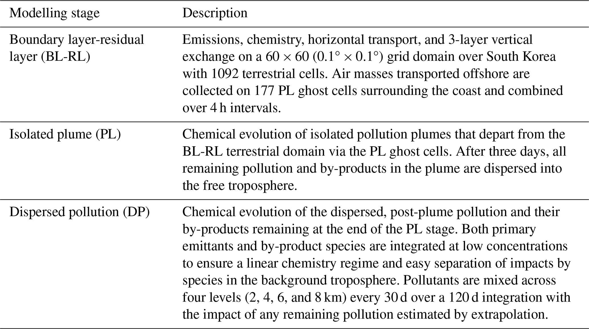
We calculate the global change in the production of tropospheric ozone (O₃) and loss of methane (CH₄) caused by 45 d of summertime South Korean anthropogenic emissions during the Korea-US Air Quality (KORUS-AQ) mission. Our modelling system consists of three stages: the boundary layer-residual layer (BL-RL) stage processes the emissions, photochemistry, deposition, aerosol reactivity, and transport over terrestrial South Korea at 0.1° × 0.1° with hourly resolution. The plume (PL) stage continues to integrate the chemistry of air masses from the BL-RL stage as they are transported offshore, simulating offshore pollution plumes observed by aircraft. After three days of chemical aging in non-diluting plumes, the pollution remnants are dispersed (DP stage) into the background atmosphere and integrated until the pollution disappears. Net O₃ production is diagnosed in each stage using the integrated ozone change and our calculated perturbation lifetimes. In total, these 45 d of South Korean emissions create an excess CH₄ sink of 4.3 Gmol and a net O₃ source of 31.2 Gmol. A simplistic scaling of these values to annual global anthropogenic emissions suggests around 10 % of CH₄ loss and 30 % of net O₃ production is attributable to anthropogenic air pollution, but our Korean summertime case exaggerates these proportions. Reducing plume aging time to 2 d increases these terms by about 10 %, and immediate dispersion (no plume aging) more than doubles them. Our model supports the typical result that rapid dispersion of pollution, e.g. through coarse resolution, overestimates its impact on tropospheric O₃ and CH₄.

1 Introduction

The degree of future climate change depends on the trajectory of tropospheric ozone (O₃) and methane (CH₄), which are potent greenhouse gases (GHGs). The primary cause of increasing CH₄ abundance over the industrial era is through direct emissions from agriculture and fossil fuel use (see review by Saunois et al., 2025). Secondarily, through the emission of short-lived air pollutants like carbon monoxide (CO), we have altered the dominant atmospheric sink of CH₄, that is, reaction with the hydroxyl radical (OH, e.g., Isaksen and Hov, 1986). Ozone has no primary emissions; its abundance depends mostly on the balance between atmospheric photochemical production and loss. Anthropogenic emissions, especially nitrogen oxides (NO_x= NO + NO₂), volatile organic carbon compounds (VOCs), and CO, drive excess production and increasing abundances of O₃ (Lin et al., 1988). Tropospheric O₃ observations from remote sites, aircraft, ozonesondes, and satellites (Gaudel et al., 2018; Ziemke et al., 2019) suggest an increase in global tropospheric O₃ background levels from the 1990s to the 2010s with a pronounced positive trend over East Asia, where O₃ precursor emissions have intensified. Observed trends in the OH-CH₄ loss rate are ambiguous but most models suggest an increase from 1980 to 2014 of order 10 % that is linked to rising NO_x emissions, especially in the lower latitudes (Stevenson et al., 2020) caused by rapid industrialisation in East Asia over the last few decades.

Previous chemistry-transport model studies of East Asian air pollution, such as Wild et al. (2004), found that “ozone formation in the boundary layer and free troposphere outside the region of precursor emissions dominates total gross production from these sources in springtime, and that it makes a big contribution to the long range transport of ozone, which is greatest in this season.” These studies, and subsequent global modelling studies of O₃ production from air pollution (e.g., Griffiths et al., 2021), have relied on the concept of odd-oxygen for separating production and loss terms, but this approach gives false lifetimes and incorrectly diagnoses production rates and their sensitivities, as recently demonstrated by Prather and Zhu (2024). These global models would have correctly calculated the perturbation to O₃ but would have incorrectly diagnosed the production and loss budgets. Here, we design a three-stage modelling system that explicitly calculates perturbation lifetimes of O₃ and can thus diagnose the net production of O₃, and loss of CH₄, that is directly caused by pollutants. The first boundary layer-residual layer (BL-RL) modelling stage tracks the initial chemistry and transport of pollution in the BL and overlying RL over South Korea. The second isolated plume integration (PL) stage follows air masses that escape from the terrestrial BL-RL domain as pollution plumes in the free troposphere (FT). The third dispersed pollution (DP) stage simulates the final chemical decay of pollution after dispersion of the plumes into the background atmosphere. The O₃ and CH₄ budget terms are extracted from the three modelling stages. We can separately calculate the O₃ budgets from pollution plumes as regularly seen by aircraft downwind of pollution sources (Bourgeois et al., 2020, 2021; Cho et al., 2021; Guo et al., 2023; Hsu et al., 2004; Jacob et al., 2003), a noted problem in Wild et al. (2004).

The test case here uses an intensive set of air pollution data and analysis from the Korea-United States Air Quality (KORUS-AQ) mission, which focused on pollution in South Korea during May–June 2016. KORUS-AQ has generated an extensive body of research on what controls the boundary layer air pollution, particularly O₃, over South Korea (Crawford et al., 2021; Eck et al., 2020; Lee et al., 2022; Miyazaki et al., 2019; Park et al., 2021; Peterson et al., 2019; Schroeder et al., 2020). We use KORUS-AQ data with our new modelling approach to quantify the global impact of this pollution on GHG budgets. The data and tools needed for our modelling system are described in Sect. 2, then the overall model and its sequence of calculations, in Sect. 3. In Sect. 4, we sum the full life-cycle impacts of the Korean emissions on the global GHG budgets and report on the GHG perturbations to tropospheric O₃ and CH₄ caused by 5 weeks of early summer Korean pollution, with the conclusion in Sect. 5.

2 Modelling components and datasets

For the three modelling stages (BL-RL, PL, and DP; see Table 1), we put together (1) emissions data, (2) atmospheric composition observations for both background and polluted regions, (3) the photochemical mechanism and box model, and (4) meteorological data for South Korea over the KORUS period. These are described in the four respective subsections below.

Table 1 Brief description of modelling stages.

2.1 Emission inventories

Three inventories drive emissions of 35 species in our model: KORUS v5 (anthropogenic; Woo et al., 2020), GFED5 (biomass burning Chen et al., 2023), and MEGAN v2.10 (biogenic VOCs; Sindelarova et al., 2014; Guenther et al., 2012). These inventory choices are consistent with the multi-model KORUS-AQ study conducted by Park et al. (2021). The KORUS v5 emissions are provided on the same 0.1° × 0.1° (latitude by longitude) grid of our boundary layer (BL) modelling stage with grid-cell edges at every tenth-degree. The GFED5 (0.25° × 0.25°) and MEGAN v2.10 (0.5° × 0.5°) grid-cell edges both coincide with KORUS v5 at degrees and half-degrees. Each of our 0.1° × 0.1° model grid-cells is mapped onto the emissions grid and collects emissions in proportion to the area of each of the emission cells it spans. All emission cells are fully covered by our BL stage cells except at the coastline, where the coarser MEGAN inventories are partially cut off. KORUS v5 and GFED5 emissions are fully included however.

2.1.1 KORUS v5 urban and industrial inventories

The KORUS v5 emissions include the explicit species: NO, NO₂, CO (see Fig. 1), ethene, formaldehyde, isoprene, acetaldehyde, methylglyoxal, benzaldehyde, acetone, methyl ethyl ketone (MEK), diacetyl, cresols, phenol, methacrolein (MACR), methyl vinyl ketone (MVK). The inventories also include SAPRC lumped species, which we represent with select surrogate species (see Carter, 2010 for SAPRC-07 documentation). We estimate molar emissions for individual species within SAPRC lumped emission categories using measured abundance ratios from NASA DC-8 airborne BL observations supplemented by emission ratio estimates in the Los Angeles basin (see de Gouw et al., 2017). Specifically, RCHO emissions go into propanaldehyde; ALK1, into ethane; ALK2, into propane; ALK3, into n-butane; ALK4, into ($\mathrm{3}/\mathrm{4}$) n-pentane + ($\mathrm{1}/\mathrm{4}$) n-hexane; ALK5, into n-heptane; ARO1, into ($\mathrm{2}/\mathrm{3}$) toluene + ($\mathrm{1}/\mathrm{3}$) benzene; ARO2, into ($\mathrm{2}/\mathrm{3}$) m-xylene + ($\mathrm{1}/\mathrm{3}$) 1-2-4-trimethylbenzene; OLE1, into propene; OLE2, into butadiene. The KORUS v5 emission inventories used in our BL-RL stage are monthly means, but the sources have variability over diurnal- and weekly- cycles, driving a nonlinear response to boundary-layer air chemistry. We therefore apply a unique temporal profile (i.e., a diurnal and week-day activity scale factor; see Crippa et al., 2020) for each BL-RL grid cell based on the different sectoral emissions in each cell (see Fig. S1 and Table S1 in the Supplement).

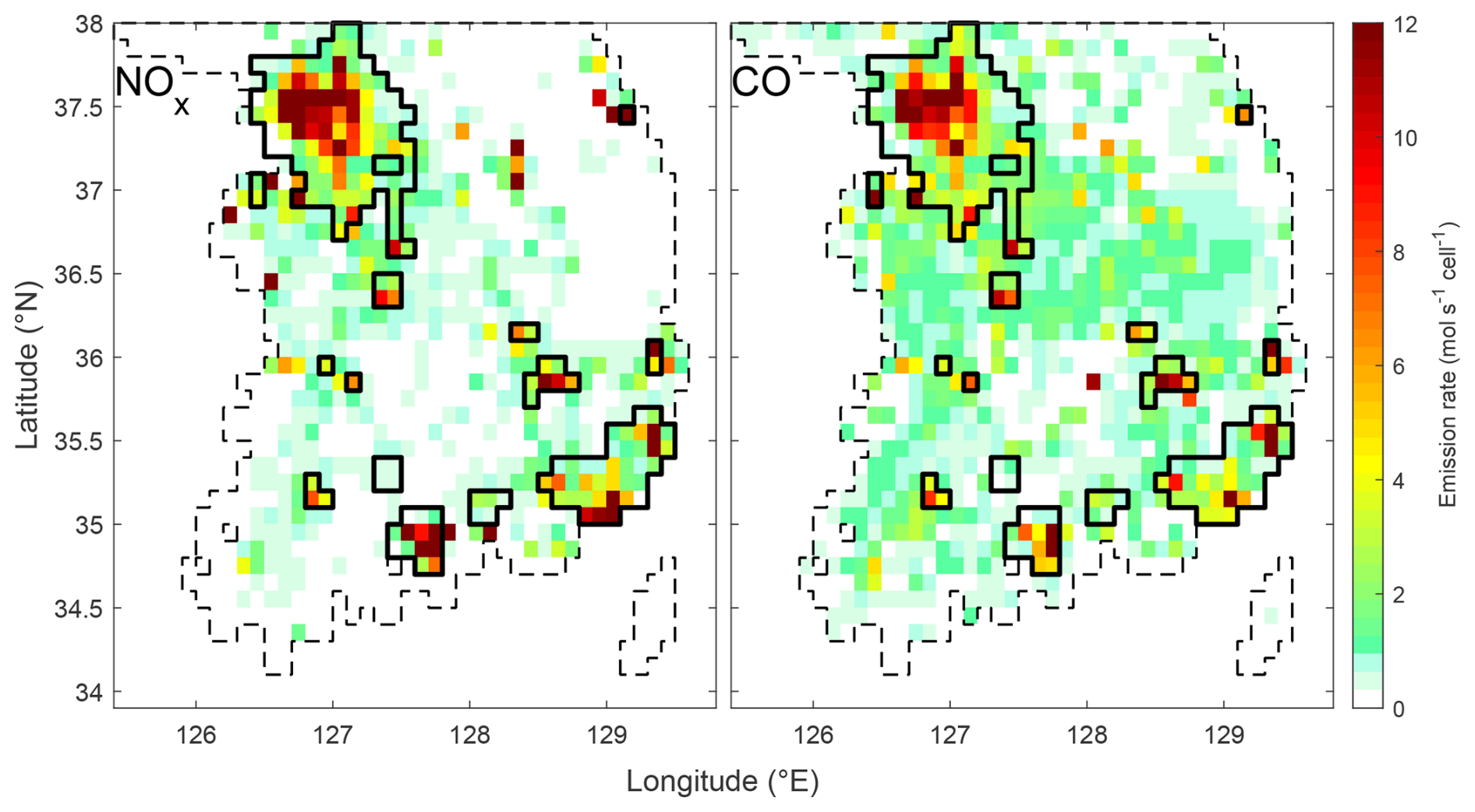
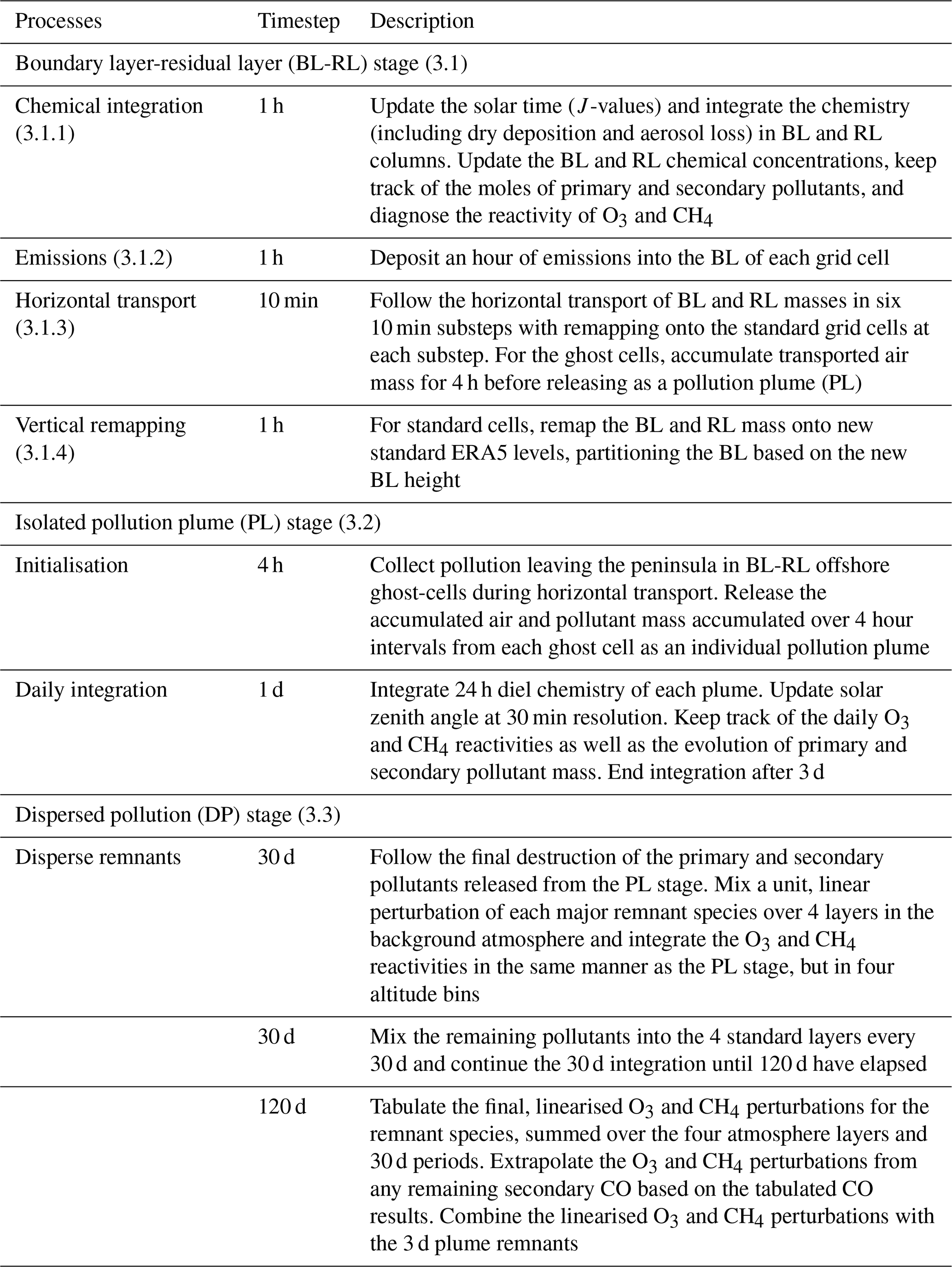
Figure 1 The May 2016 NO_x and CO anthropogenic emission rates from the KORUS v5 inventory (Woo et al., 2020) shown as coloured cells (Same units apply to NO_x and CO). Bold lines enclose “urban” grid-cells in our model-observation comparison that were effectively monitored by five or more NIER ground stations within a ten-kilometre locus during the KORUS-AQ period (see Wilson and Prather, 2025 for ground station distribution). Dashed lines enclose the BL-RL terrestrial domain.

2.1.2 GFED5 biomass burning inventories

We used daily-resolved May and June 2016 biomass burning inventories from GFED5 (0.25° × 0.25°, g m⁻² d⁻¹; see Chen et al., 2023), assuming temporally uniform emissions. We include GFED5 emissions of NO, CO, ethane, propane, ethene, propene, isoprene, MEK, benzene, toluene, xylenes (as m-xylene), methanol, ethanol, formaldehyde, acetaldehyde, propanaldehyde, methyl glyoxal, formic acid, and glycoaldehyde. We consider the GFED5 inventories as part of the anthropogenic perturbation alongside KORUS v5, assuming the emissions are predominantly from agricultural waste burning.

2.1.3 MEGAN v2.10 biogenic inventories

We use monthly mean MEGAN v2.10 biogenic emission inventories with constant temporal profiles generated for May and June 2010 (0.5° × 0.5°, kg m⁻² s⁻¹; see Guenther et al., 2012). We use the following inventories: CO, ethane, propane, ethene, propene, isoprene, toluene, ethanol, formaldehyde, acetaldehyde, acetone, and acetic acid. As in the GFED5 inventories, offshore emissions are assumed to be negligible and excluded from the BL-RL stage.

2.2 In situ observations

Observations are used to define the clean-air background chemical composition in our modelling system. The BL-RL stage (Sect. 3.1) uses airborne KORUS-AQ measurements (KORUS-AQ Science Team, 2019) to prescribe a single background composition as a boundary condition for free tropospheric air entrained into the terrestrial BL and RL. Note that our use of a single average KORUS-AQ background composition does not resolve variations in transboundary O₃ and CO pollution entering the Korean peninsula as observed by Miyazaki et al. (2019). In the final stage of our modelling sequence (DP stage), we disperse plumes into a vertically-binned remote background environment obtained from the Atmospheric Tomography Mission (ATom) (Sect. 3.3). Our primary model-observation metrics compare the BL concentrations in our 0.1° × 0.1° grid cells with a grid-cell averaged values of O₃, CO, and NO_x as observed at the surface NIER sites. See Wilson and Prather (2025) for the methodology of deriving grid-cell averaged data from a set of sites.

2.2.1 KORUS-AQ airborne observations

NASA DC-8 sampled the air above South Korea and the Yellow Sea during 20 d between 1 May and 11 June 2016. Flight paths were coordinated to follow Seoul pollution and other plumes (e.g., from the Daesan industrial complex), and thus distributions of pollutants are positively skewed as a result. All species mole fractions show a clear peak probability at low percentiles, which we use to define “background” air. We calculate the modal concentrations using the Half-Sample Mode of all South Korean flight data and use them to define the BL-RL background composition. These values are not sensitive to the inclusion or exclusion of data sampled within the ERA5-defined boundary layer (Hersbach et al., 2023).

We also use KORUS-AQ observations of photolysis frequencies (J-values) and aerosol surface area densities in our chemistry modelling and describe these data and their usage in Sect. 2.3.2 and 2.3.3.

2.2.2 ATom airborne observations

The ATom missions deployed the DC-8 to sample the air over the remote ocean basins and profile the reactivity in the troposphere (Thompson et al., 2022). We define the DP background compositions using 10 s merged ATom-4 data (27 April, 29 April, and 21 May 2018) from the modelling data stream (Prather et al., 2023) sampled to represent summer Pacific conditions. We take the medians of data partitioned into 2-km-wide altitude bins, centred on 2, 4, 6, and 8 km, using only data flagged as primary and secondary observations; the medians were used to spin-up the DP background air over 365 d (constant summer conditions) in the respective altitude bins (see Table 2 for spun-up concentrations).

Table 2 Background air compositions used in the modelling system.

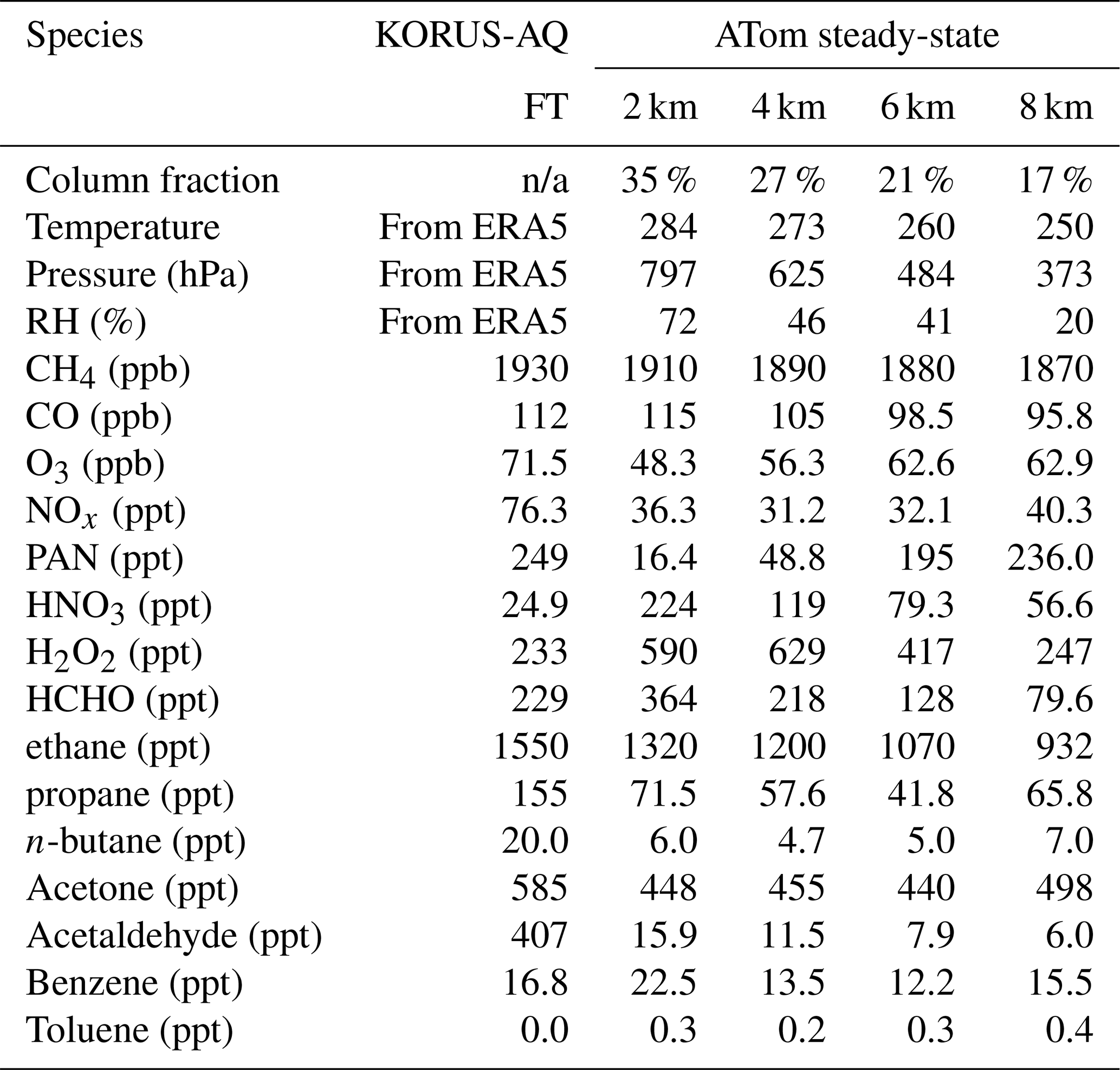
The KORUS-AQ FT (free troposphere) composition provides background air to the BL-RL stage and is derived from the Half-Sample Mode of South Korean DC-8 flights. The ATom data are steady-state background compositions used in our DP stage (Sect. 3.3). ATom flight data were sampled on 27 and 29 April, and 21 May 2018 between 30–50° N and 200–235° E, the median 10 s values over 2 km-wide altitude bins centred on 2, 4, 6, and 8 km are used here. Some very low-abundance VOCs (e.g., C₂H₄, isoprene, n-C5-7 alkanes) are initialised in the BL-RL stage but not tabulated here. n/a = not applicable.

2.2.3 NIER surface pollution maps

Surface observations of O₃, CO, and NO_x were recorded by South Korea's National Institute of Environmental Research (NIER) network of 300+ ground stations from 2 May 2016 to 11 June 2016. These measurements have been spatially interpolated via inverse distance weighting (discussed in Wilson and Prather, 2025) and gridded to match our BL-RL stage resolution (available at Wilson, 2026).

2.3 Photochemical box model

In all stages of our modelling system we integrate the photochemical evolution of air masses containing South Korean air pollution. For this, we implement the Framework for 0-D Atmospheric Modelling (F0AM v3.1; Wolfe et al., 2016) using explicit chemical mechanisms described in Sect. 2.3.1. F0AM is initialised with the mole-fractions of all the chemical species, with constant meteorological parameters (temperature, pressure, and relative humidity), and with J-values that we derive from KORUS-AQ observations. Meteorological parameters (pressure and temperature) are used to compute the rate coefficients. During the BL-RL stage, the F0AM chemistry and meteorology is reinitialised hourly in the BL and RL of each grid cell before emissions and transport. During the PL and DP stages, the F0AM model is run over longer periods in a diel cycling mode, updating the J-values every half-hour based on the computed solar zenith angle at a standard point near Seoul (37.5° N, 127° E).

2.3.1 Chemical mechanism

From our set of 35 emitted species, we generate a chemical system of 1610 chemical species and 5000 reactions using the Master Chemical Mechanism (MCM v3.3.1; Bloss et al., 2005; Jenkin et al., 1997; Jenkin et al., 2003; Jenkin et al., 2015; Saunders et al., 2003). Most of these species are secondary VOCs branching from the decomposition pathways of the primary species.

We found that incomplete reaction mechanisms led to some spurious results in our dispersed pollution modelling. Notably, residual benzene pollution catalysed ozone depletion through secondary products (2-hydroxyphenoxy radical, 2-phenol peroxide, and phenol hydroperoxide) that had an extremely slow termination path. We solved this problem by introducing a first-order loss with a lifetime of 5 d for organic hydroperoxides and hydroxylated species based on the wet deposition timescale for gases with large Henry's Law constants (Bi and Isaacman-VanWertz, 2022). This loss was also included for HNO₃ to avoid unrealistic accumulation in the DP stage.

2.3.2 Photolysis frequencies

We use KORUS-AQ observations of J-values under all-sky conditions to model photolysis in our chemical box model (see Hall et al., 2018 for instrumental details). We computed the mean J-values centred in 5° solar zenith angle (SZA) bins (15 to 60° bin edges), sampling observations below 1.5 km for the BL-RL stage, and above 1.5 km for the PL and DP stages. To simulate the diurnal cycle of J-values, F0AM uses the MCM parameterisation: $J=J_{\mathrm{MCM}}\cos \left(\mathrm{SZA}{)}^m\exp \right(n/\cos \left(\mathrm{SZA}\right)$), where J_MCM, m and n are reaction-specific fitting parameters originally obtained from clear sky radiation modelling (Jenkin et al., 1997; Saunders et al., 2003). Here, we use our SZA-binned KORUS-AQ observations to derive more realistic all-sky J-values: J_KORUS=k J_MCM, providing F0AM with the correction factors k. We did not attempt to correct the J_MCM values that were not observed by DC-8 as these tend to be far less important, low abundance species. See Table 3 for the list of J_KORUS and J_MCM scale factors, and Fig. 2 for a sample of observed vs. fitted (J_KORUS) J-values as a function of SZA.

Table 3 The photolysis reactions recalibrated in our modelling system.

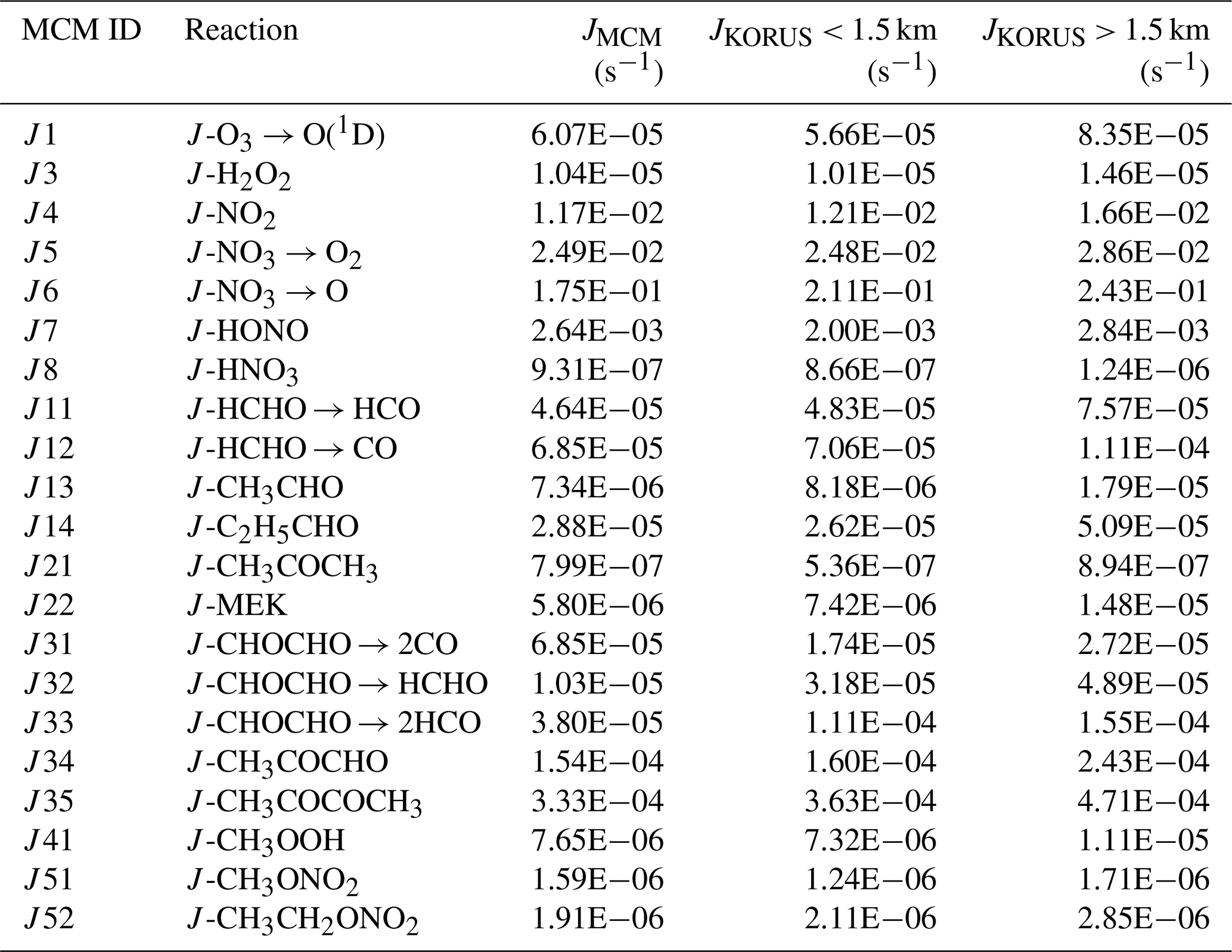
J_MCM values are the clear-sky J-value coefficients used in MCM (Saunders et al, 2003). J_KORUS are the all-sky coefficients used in our modelling system, fitted using KORUS-AQ J-value observations. MCM also includes photolysis reactions of n- and i-propylnitrate, t-butylnitrate, 2-oxopropyl nitrate, n-butyraldehyde, i-butyraldehyde, (Z)-4-hydroperoxy-2-methyl-2-butenal, MACR, and MVK, which were not reported in KORUS-AQ data.

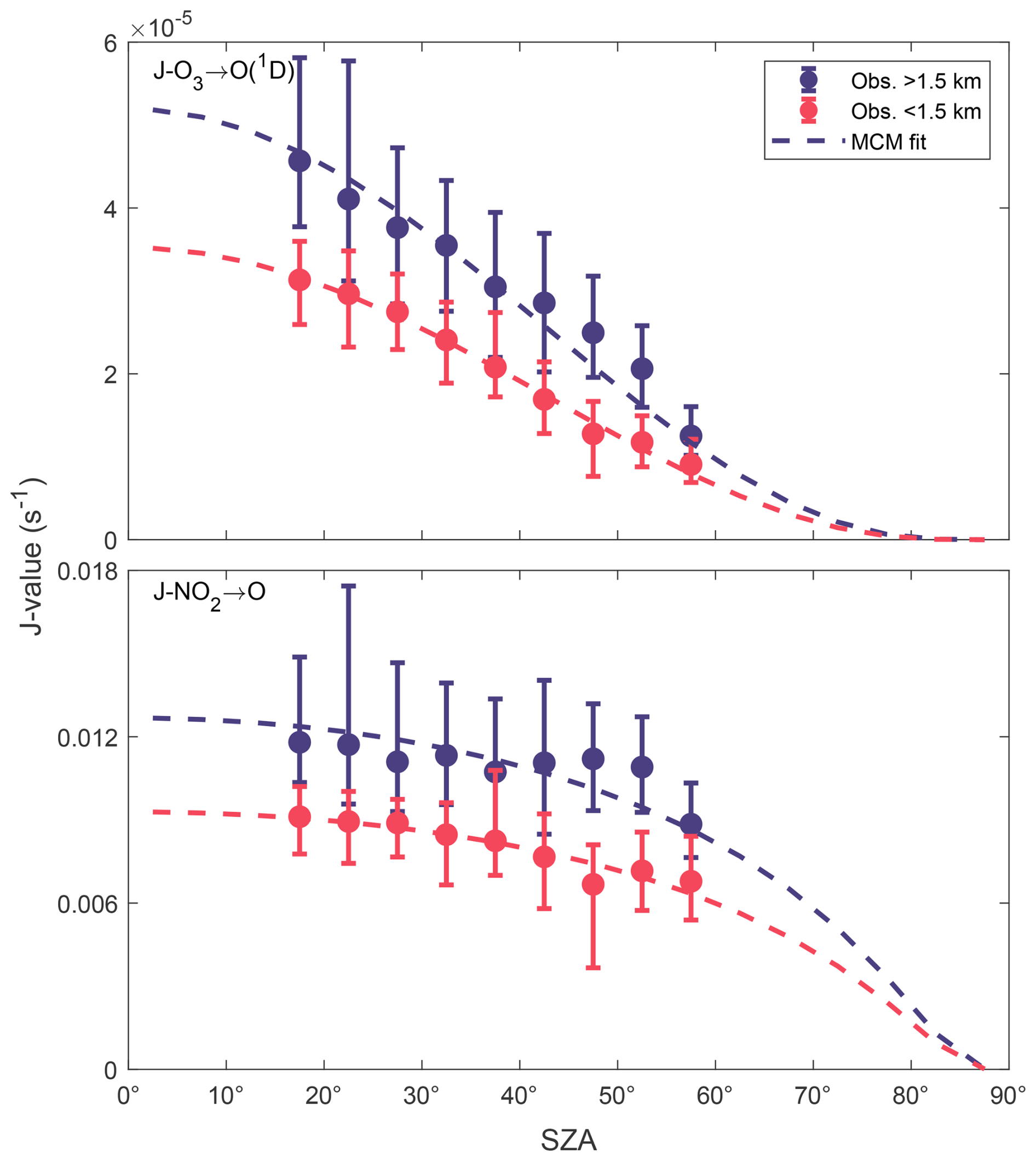
Figure 2 Observed and fitted all-sky J-O₃–> O(¹D) and J-NO₂ photolysis frequencies. Dots show the mean J-values in 5° SZA bins and whiskers show the root mean square deviations of the upper- and lower- residuals. Dotted lines show the MCM-parameterised J-values scaled to J_KORUS values. Data were sampled above (blue) and below (orange) 1.5 km altitude.

MCM v3.3.1 lacks a photolysis mechanism for peroxyacetyl nitrate (PAN), which is important for PAN loss only in the DP stage in the upper troposphere. We added J-PAN as being proportional to J-O₃→ O(¹D) with scale factor 0.014 based on the KORUS J-values and empirical PAN photolysis frequencies (Talukdar et al., 1995).

2.3.3 Aerosol reactivity

Hydrolysis of N₂O₅, NO₂, and NO₃ on aerosol surfaces is an important sink for NO_x in a polluted environment, effectively converting NO_x to HNO₃, which is irreversible in the BL-RL and PL stages. Aerosol-HO₂ reactions also reduce HO_x (OH + HO₂) and subsequently ROOH radicals. The first-order rate coefficient for aerosol reactivity with molecule X is given by $(\mathrm{1}/\mathrm{4}){\mathit{\rho }}_{\mathrm{A}}{v}_X{\mathit{\gamma }}_X$ (Yan et al., 2019), where ρ_A is aerosol surface area density, v_X is the mean thermal velocity of X, and γ_X is the surface reaction probability. We use Lamarque et al. (2012) aerosol reactivities (${\mathit{\gamma }}_{{\mathrm{N}}_{\mathrm{2}}{\mathrm{O}}_{\mathrm{5}}}=$ 0.1; ${\mathit{\gamma }}_{{\mathrm{NO}}_{\mathrm{2}}}=$ 0.0001; ${\mathit{\gamma }}_{{\mathrm{NO}}_{\mathrm{3}}}=$ 0.001; ${\mathit{\gamma }}_{{\mathrm{HO}}_{\mathrm{2}}}=$ 0.2), which are taken to be independent of aerosol composition. Aerosol surface area densities were inferred from KORUS-AQ Laser Aerosol Spectroscopy (LAS) in situ 10 s measurements of size-resolved particle number density (Nault et al., 2018). We average the surface area densities over the entire KORUS-AQ period for altitude ranges of 0.0–1.5 km (BL-RL stage), 2±1 km (PL and DP stages), 4±1, 6±1, and 8±1 km (DP stage). Thermal velocities for the four species were computed using the mean ERA5 meteorology for the BL-RL stage and ATom mean temperature profiles for PL and DP stages (see Table 2). Final aerosol reactivity values used in the different modelling stages are shown in Fig. 3.

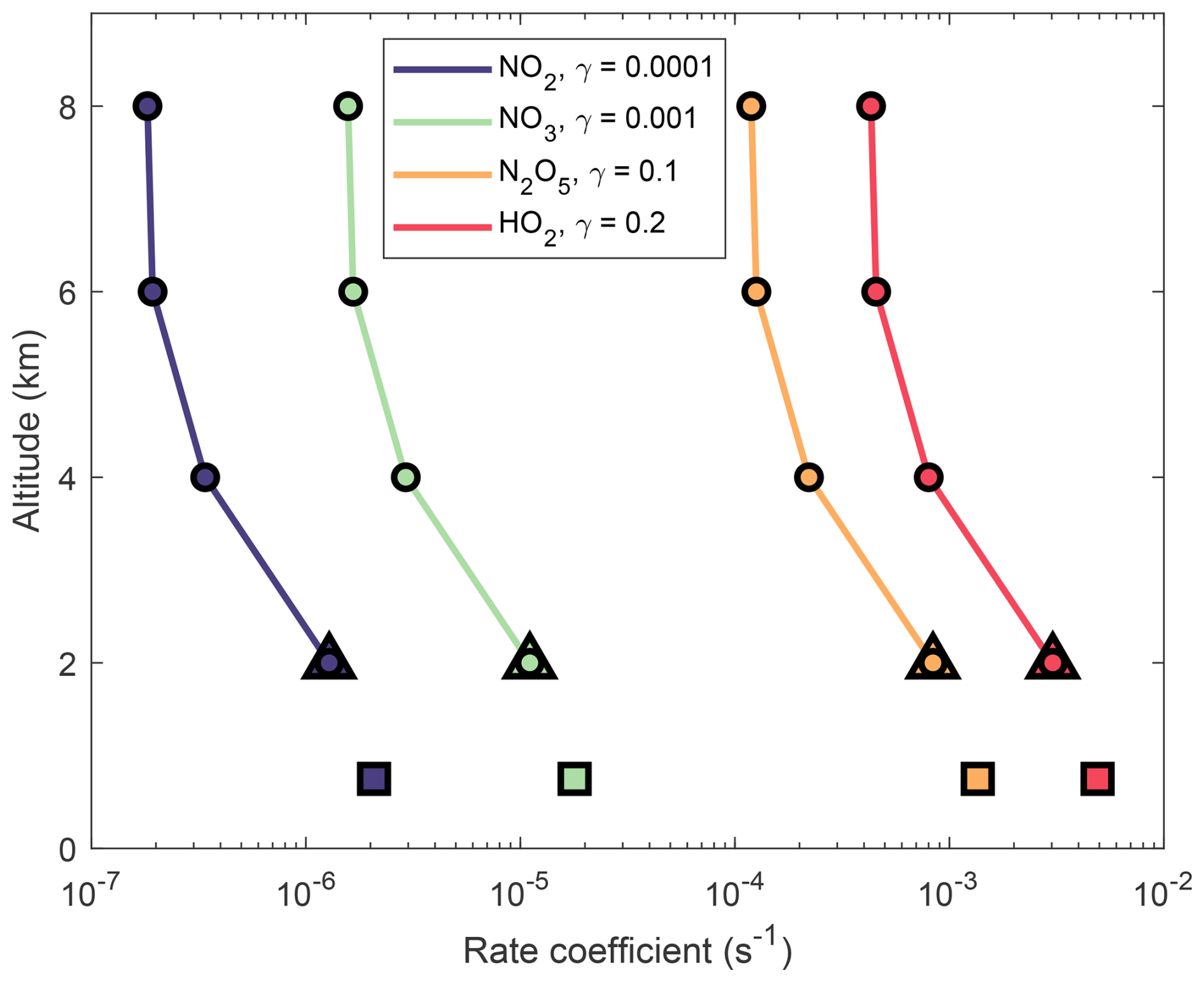
Figure 3 Aerosol reactivity rate coefficients used in our model stages. These first-order loss coefficients for NO₂, NO₃, N₂O₅, and HO₂ are computed from mean aerosol surface area concentrations and temperatures profiled by DC-8 during the KORUS-AQ mission and used for the BL-RL (squares; 0.0–1.5 km altitude), PL (triangles; 2±1 km), and DP (circles; 2±1, 4±1, 6±1, and 8±1 km) stages (see Table 2). Aerosol surface areas are from KORUS-AQ LAS data (Nault et al., 2018).

2.3.4 Surface deposition

Surface deposition is a sink of O₃ and NO₂ in our hourly BL chemical integrations. The BL-RL stage uses a simple dry deposition velocity (v_d, cm s⁻¹) for O₃ and NO₂ in each grid cell based on a fixed land surface classification over the KORUS period. The deposition first-order loss rate (s⁻¹) in the BL is calculated hourly as v_d divided by BL height (cm). To map the land cover over the BL-RL grid domain, we use 32 land cover classifiers as defined by the Land Cover Classification System (LCCS; Copernicus Climate Change Service, Climate Data Store, 2019). From the LCCS $\mathrm{1}/\mathrm{360}$° × $\mathrm{1}/\mathrm{360}$° pixels, we calculate the fractional coverage of each classifier in our 0.1° × 0.1° model cells. We group the 32 classifiers into 8 super-classifications used by Jia et al. (2016) (see Table 4 for our super-classifications and their constituent LCCS classifiers). We combine our classification fractional areas to calculate average v_d values for O₃ and NO₂ as shown in Fig. 4.

Table 4 Average dry deposition velocities (v_d) for land surface categories.

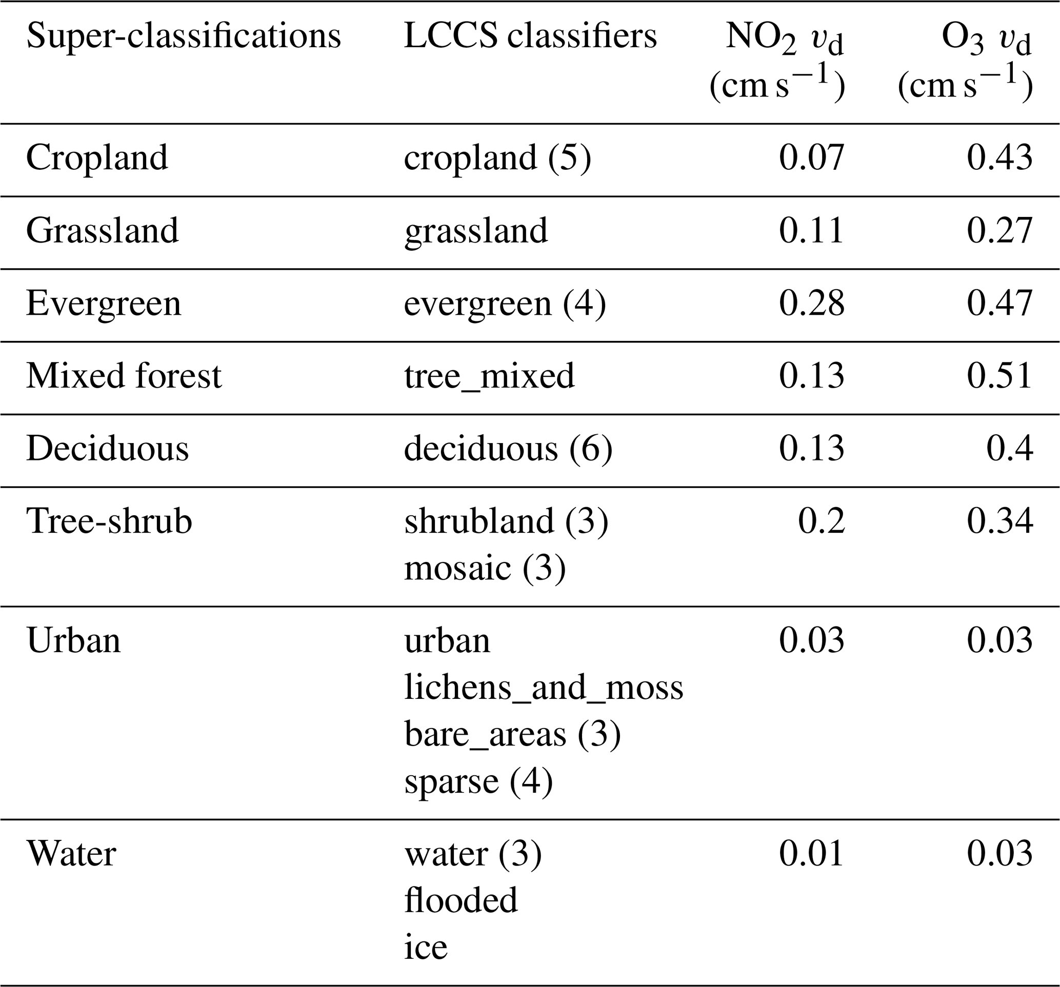
Values shown are based on data from field campaigns covering different terrain classifications (Zhang et al., 2009; Adon et al., 2013; Zhang et al., 2002; Simpson et al., 2001; Brook et al., 1999). Data represent diel averages over the campaign periods. For super classifications with the LCCS classifiers, see text.

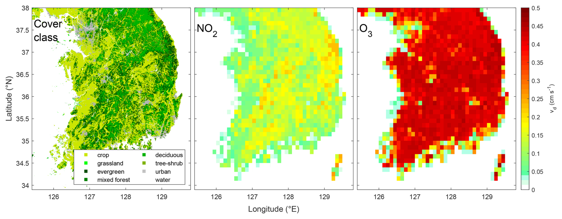
Figure 4 Land cover classes and dry deposition maps. Land cover classes show our super classifications based on the LCCS classifiers plotted at the native $\mathrm{1}/\mathrm{360}$° × $\mathrm{1}/\mathrm{360}$° resolution (left). Dry deposition (v_d) rates for NO₂ (middle) and O₃ (right) at model resolution (0.1° × 0.1°) are derived from the area-weighted super-classifications and average deposition velocities in Table 4.

2.4 ERA5 meteorology

Our BL-RL stage uses hourly, 0.25° × 0.25° ERA5 Reanalysis 2D fields for boundary layer height and surface pressure (Hersbach et al., 2023) plus 3D fields for temperature, specific humidity, u, and v wind (Hersbach et al., 2017). The ERA5 data are point-values defined at grid centres (e.g. 37.50° N, 127.00° E at Seoul) and at hybrid (η) vertical level centers. ERA5 pressure is indexed on vertical level edges. Our BL and RL columns are discretized and vertically aligned with these edge-level coordinates at the start and end of every hourly timestep in the model, and the 3D fields are averaged separately in the BL and RL columns to produce 2D mean column values for winds, temperature, and humidity. We only use the lower atmospheric ERA5 data, from k= 99 (∼4.5 km altitude) to k= 137 (surface; see Table S2).

The BL always consists of at least one ERA5 layer above the surface, and the RL – if it exists – consists of at least one layer atop the BL column. The BL and RL columns each have a single chemical mixture with a mean pressure and temperature averaged over their constituent ERA5 layers. To obtain these fields at model resolution (0.1° × 0.1°), we interpolate the grid-centred ERA5 data to our model grid-cell centres via bicubic convolution and assume these data points represent the area mean. The ERA5 nocturnal BL height falls to a mean minimum height of 175 m over the Korean peninsula, and locally as low as 24 m, leading to unrealistically concentrated emissions. We mitigate this problem by prescribing a minimum BL height of 200 m in our model.

2.4.1 Vertical discretisation (BL and RL)

Our BL-RL stage uses mass-weighted (δp) column averages for temperature, specific humidity, and horizontal wind fields. To average these variables for the BL and RL, we align the BL and RL edges in our model to nearest ERA5 vertical edge levels in each gridded interpolated ERA5 atmospheric column over the terrestrial domain. Each model time step starts and finishes with a discretised BL + RL column, where the BL consists of an integral number of ERA5 levels based on mass, and the RL, if it exists at the time, consists of an integral number of ERA5 levels atop the BL. When the ERA5 BL height (m) changes with time, we adjust the top of the BL to the closest ERA5 edge level (in metres). If the BL column expands to envelop higher levels, it collects all the pollution in the entrained RL levels; if it envelops levels above the RL, it collects FT air. If the BL contracts, it leaves behind discrete layers of residual pollution that are mixed with the RL column. This step represents the effective vertical transport in the model.

When the ERA5 surface pressure field changes each hour, the ERA5 edge-level pressures shift, resulting in misaligned initial and final pressure levels. This effect is hardly noticed because the horizontal transport of BL and RL levels separately results in BL and RL mass that do not align with the new edge levels. Every hourly timestep, after horizontal and vertical transport, we realign the BL-RL and RL-FT (or BL-FT) interfaces with the standard ERA5 levels (rediscretisation) and remap the air mass from the intermediate BL + RL + FT columns to the new partition (remapping). The BL and RL masses adjust during horizontal transport. If the new BL mass (determined by the new BL height and ERA5 level edges) exceeds the transported BL + RL burdens, then the RL is fully entrained and some FT air is remapped to the BL. If the transported BL + RL mass exceeds the new BL mass, then some air is remapped into the RL. If any RL mass remains after vertical transport, the RL-FT interface is rediscretised by adding the ERA5 levels upward from the new BL-RL interface to the first level that fully encapsulates the RL mass. Some background FT air is remapped to the RL during this process. While we keep track of the BL and RL air mass during horizontal transport and vertical remapping, the critical elements being transported are the moles of primary and secondary pollutants. When we add FT air to the BL or RL, we likewise keep track of the pollutants from this relatively clean air. During this process, no pollutants are mixed into the FT: the accumulated pollutants, including those emitted into the BL and entrained from the FT, can only leave the South Korean peninsula horizontally as polluted plumes to be tracked in the PL stage.

We calculate the temperature and specific humidity of the BL and RL in each grid-cell as mass-weighted averages. Horizontal wind velocities in the BL and RL are also -mass-weighted at ERA5 grid centres, but we compute column-averaged winds over the same set of levels over the entire peninsula to avoid spatial discontinuities. For each timestep, BL winds are vertically averaged from the surface to the median top-of-BL level, and RL winds, from the median top-of-BL level to the median top-of-RL level.

3 Modelling system

The hybrid modelling system is quasi-three-dimensional, accounting for the geographic variations in BL pollution over South Korea. The modelling system follows the chemical evolution of boundary layer pollution as it travels across South Korea (BL-RL stage), continues to chemically age the air masses leaving the peninsula as isolated pollution plumes (PL stage) and finally as dispersed pollution remnants (DP stage) under realistic, but idealized, atmospheric conditions typical of the region. The BL-RL stage is the most complex, using hourly emissions and meteorology to model the chemical evolution of pollution in the planetary boundary layer as it moves across the South Korean peninsula (see Table 5). We do not explicitly consider the convective transport of BL pollution directly into the FT. Large convective systems lift and disperse BL pollution in reality; however, we follow the horizontal pollution transport evolution across the peninsula and offshore into the PL stage.

Table 5 A summary of the modelling operations acting on South Korean air pollution.

The discrete processes for the three modelling stages are outlined and briefly described. The timesteps indicate the frequency at which operations are performed.

The PL stage chemically ages the pollution when BL or RL air masses are first swept offshore. This pollution is collected over 4 h intervals in BL-RL ghost cells surrounding South Korea, then released as isolated pollution plumes to evolve undiluted for 3 d at 2 km altitude. When these plumes disperse, the remaining primary and secondary pollutants (including O₃) are passed to the dispersed pollutant (DP) stage. Here, we assume that pollutants are dilute enough that the chemical response is first-order with respect to the number of moles of dispersing pollutant, and can be calculated separately for each species based on the observed background composition of the mid-latitude Pacific troposphere. Each pollutant's impact is independent of the other pollutants. The DP stage mixes the remaining pollutants from the PL stage uniformly across the 1–9 km altitude range and calculates the O₃ and CH₄ budget terms across four altitude ranges (2±1, 4±1, 6±1, and 8±1 km) to. Every 30 d the pollutants are remixed vertically. After 120 d the chemically active pollutants are mostly gone and a simple extrapolation from the last 30 d can be used to estimate any remaining O₃ and CH₄ reactivity. The sequence of modelling operations is summarised in Table 5, and details of the calculations are described below.

3.1 Boundary layer-residual layer (BL-RL) stage

The BL-RL stage is set on a latitude-longitude grid of 60×60, 0.1° × 0.1° geographical cells centred on South Korea. The BL-RL domain comprises 1092 terrestrial grid-cells where emissions and chemistry are processed, and 177 ghost-cells on the model domain circumference that collect air transported out of the BL-RL domain. When diagnosed, the BL and RL always consist of a discrete number of contiguous ERA5 layers. The BL always contains the layers from 0–200 m above surface, while RL may be completely absent if fully entrained by the BL, or fully ventilated by horizontal transport. The chemical concentrations in the BL and RL are calculated from the tracked number of moles of pollutants, and the molar dry air column burdens, which are proportional to the sum of the δp levels (see Table S2) and grid-cell quadrangle areas.

Within the model domain, the BL and RL columns in each cell have a unique mix of pollutants, with a single pressure, temperature and chemical composition. The BL collects, transports, and chemically evolves fresh emissions while depositing O₃ and NO₂ to the surface. The RL collects, transports, and chemically evolves air detrained from the BL when the BL height drops. All air outside the terrestrial cells and in layers above the BL + RL has FT background composition, and this air can enter the BL columns when the BL height rises above the RL layer, or when offshore air is horizontally transported into the terrestrial grid cells.

3.1.1 Photochemistry

The first modelling step in the BL-RL stage is the F0AM integration of hourly chemistry for each BL and RL column. F0AM integrates the chemistry in each column using the pollutant mixing ratios, MCM v3.3.1 rate coefficients, first-order deposition rates (dry, aerosol, and scavenging), mean column meteorology (temperature, pressure, relative humidity), SZAs computed from grid-cell coordinates and model UTC time, and KORUS-AQ all-sky J-values (see Sect. 2.3–2.4). Temperature and pressure are used to calculate the reaction rates and convert mixing ratios to number densities. Budget data such as chemical tendencies and individual chemical rates are integrated at the sub-hourly F0AM ODE solver resolution and diagnosed every hour.

3.1.2 Emissions

Each hourly timestep, after the chemical integration, we inject an hour of emissions into each grid cell given the species-wise emission rates (mol s⁻¹) of the KORUS v5, GFED5, and MEGAN v2.10 inventories (see Sect. 2.1.1–2.1.3). For the KORUS v5 inventories, we multiply the mean emission rate (resolved monthly) by a diurnal activity scale factor (resolved hourly) and a day-of-week activity scale factor (weekday, Saturday, or Sunday). These scale factors are unique to each grid cell and derived from the individual emission sector activities in the cell (see Sect. 2.1.1).

For cells with intense emission sources, the operator splitting poses a challenge. If we release an hour of emissions into each grid-cell before the chemistry operator, then the hour-long chemistry calculation begins with a mass of unrealistically concentrated, undispersed air pollution rather than a ventilated stream of emissions processed continuously. With our current operator sequence, the emissions are transported partly to neighbouring cells before the chemical generation of secondary pollutants. The obvious remedy is to cut the overall operator time-steps to e.g. 30 min or even 10 min. Unfortunately, restarting the chemistry integration every 10 min is computationally prohibitive for us. However, we can test the errors caused by our operator sequencing by cutting the overall time step to $\mathrm{1}/\mathrm{2}$ and $\mathrm{1}/\mathrm{4}$ h for a 3 d test case. From 1 to $\mathrm{1}/\mathrm{4}$ h timestepping, we found a +1.3 % and +0.9 % error in total CH₄ and O₃ reactivity; and from $\mathrm{1}/\mathrm{2}$ to $\mathrm{1}/\mathrm{4}$ h, the errors decrease but change sign, indicating convergence.

3.1.3 BL and RL horizontal transport

Horizontal advection moves the BL and RL across the peninsular grid, brings in FT background air from offshore, and sends pollution plumes from the model domain to the offshore PL ghost cells. Each hour, we calculate two sets of grid-resolved 2D (u, v) wind fields, one for the BL and one for the RL. We transport each on separate planes following the BL and RL (u,v) trajectories to their new locations. These trajectories are fixed over the 1 h step and are generally not straight lines. We move each BL or RL cell in a sequence of six 10 min sub-steps, where each sub-step splits the original (source) cell into four new (receptor) grid cells as depicted in Fig. 5. The four parts of the BL/RL cells are reassembled onto the standard grid cell, and the process is repeated for the remaining 5 sub-steps. Cell fractions transported offshore are collected as pollution plumes for the PL stage. The choice of 10 min advection timesteps enables intense emissions to horizontally ventilate quasi-continuously along curved trajectories over the hour.

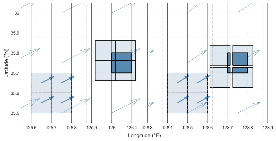
Figure 5 A schematic of the BL-RL stage horizontal transport. Left: the receptor BL column (dark-blue square) receives air mass from four source BL columns (dashed light-blue squares) transported north-eastward in a straight-line path without divergence over a 10 min step. The new receptor BL comprises a fraction of each source BL column in proportion to the rectangular overlap after transport (dark-blue rectangular areas). Right: As described above, but in a divergent wind field. The four adjacent light-blue cells separate, and the white cross-shaped area in the receptor cell is vacuous. Wind vectors (arrows) are sampled centrally in the ERA5 grid (dashed grid), vertically averaged in the BL, and interpolated to the model grid cell centroids (bold arrows) to determine the source cell trajectories.

To compute the trajectory paths for each terrestrial BL cell, we adopt a fixed effective BL height for the one-hour time step for all South Korea based on the median top-of-BL height for terrestrial cells (see Sect. 2.4.1). Using this set of fixed ERA5 levels, we calculate a pressure-weighted set of (u,v) fields at the centroids of the 60×60 model cells with bicubic interpolation. The u and v components are converted to angular velocities in per-second degree arcs that remain fixed over the 1 h time step. We then transport the BL cell to new centroid positions along the arcs via 10 min Euler-forward-stepping linear trajectories. These 10 min trajectories are linear and non-deformational and thus allow for easy partitioning into four cells at their destination as shown in Fig. 5. The series of 10 min sub-stepping trajectories allows realistic curved and deformational motion of the BL cells (i.e., convergence or divergence). Then we partition the source BL air mass (and pollutants therein) into four receptor cell BLs in proportion to the source-receptor area overlaps. This is repeated 6 times over the hour. The RL cells are transported likewise, but using the RL-weighted (u,v) fields, where the pressure-weighting of the winds ranges from the median South Korean top-of-BL level-edge to the median top-of–RL level edge.

The interpolated BL and RL (u,v) winds will almost certainly include convergence or divergence and thus receptor cells will collect more or less than 100 % of their area fractions. This discrepancy, along with the discrepancies in source- and receptor- BL column masses, leads to a change in BL + RL dry-air column masses after each 10 min step. BL and RL air mass and source cell pollution that is transported outside the terrestrial domain is accumulated in the ghost-cell closest to the transported centroid coordinates. We track BL and RL outflows to ghost cells separately, but do not vertically remap or discretise them in the ghost cell. Their chemical evolution in the PL stage is treated separately and identically. Inshore flow to terrestrial cells provides FT air to the BL in proportion to the source-receptor area-overlap and receptor BL column mass. We assume RL pollution does not mix with FT air, so we ignore offshore transport into the terrestrial RL.

3.1.4 Vertical remapping of the BL-RL

With each 1 h timestep, we have new ERA5 fields for surface pressure and BL height. As described in Sect. 2.4, the new BL height in meters is used to select the new upper BL edge-level in hPa that most closely matches it. If the BL top after horizontal transport lies above the new one (i.e., a falling BL) then the polluted air mass between the new and old BL is added to and mixed with the overlying RL, creating a new RL if none initially existed. If the new BL top lies above the new one (i.e., a rising BL) then the new BL takes in the mass from the RL. If the available RL mass is insufficient then the BL entrains mass and chemical pollutants (including O₃) from the FT. The BL-RL-FT exchange during the vertical remapping step depends on BL height dynamics (i.e., the change in BL height over the last hour), but is also convoluted by horizontal transport (i.e., convergence or divergence in BL and RL trajectories). The BL and RL columns transported into a grid-cell at the end of the time step will not align with the BL in the receptor grid-cell and model levels and must be remapped as illustrated in Fig. 6. In Fig. 6a, the new BL air mass (right column) exceeds the BL + RL masses (left column), and thus it entrains all pollutants in the BL and RL plus those in the FT needed to make up the total air mass (thick black bars). In Fig. 6b, the new BL mass sits in the middle of the transported RL, and thus some of the transported RL goes into the new BL, and the remainder, into the new RL. The new RL is rounded up to the next level by adding FT mass (and FT pollutants) into the RL. In Fig. 6c, the new BL mass is less than the transported BL mass, and the excess is placed into a new RL.

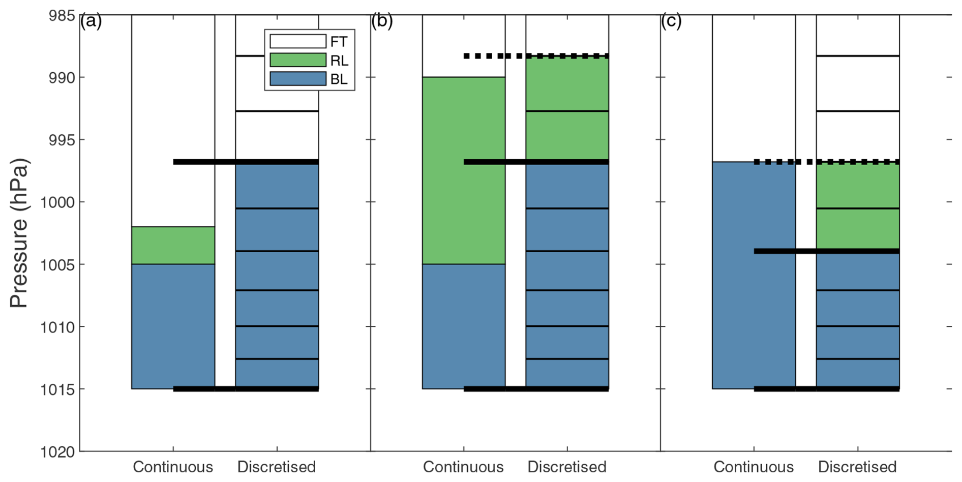
Figure 6 Schematic of the BL-RL stage vertical remapping. The four panels show the re-gridding of a BL (blue) and RL (green) air masses that have been left in a new cell after the horizontal transport step. The new cell is marked with the pressure edge levels based on the new surface pressure and a BL mass (blue) based on the new BL height; see text. Three examples here are: (a) incoming BL + RL mass is less than new BL mass, so BL + RL + FT is pulled into the new BL and the RL disappears; (b) BL + RL mass exceeds new BL mass, so some RL is absorbed into the new BL and a new, smaller RL is created with some FT air incorporated; and (c) incoming BL mass exceeds the new BL and so an RL is created.

3.1.5 Surface observations

We compare our BL results for O₃, CO, and NO_x with grid-cell averaged observations derived from the NIER network (Sect. 2.2.2) using the methodology of Wilson and Prather (2025). In Sect. S3 of the Supplement we show model-observation statistics and plots, sampled in “urban” grid-cells that were effectively observed by five or more NIER sites. The time series is decomposed into four meteorological phases described by Peterson et al. (2019), named as dynamic (1–16 May), anticyclone (17–22 May), transport (25–31 May), and rex-block (1–7 June). Our model performance and diurnal cycles for O₃, CO, and NO_x were consistent with a separate study that used the WRF-Chem v4.4 chemistry-transport model (CTM) driven by the same KORUS v5 inventory (see Table S3 and Figs. S2–S6; see Fig. 2 from Kim et al., 2024). Modelled O₃ correlated well with observations (R= 0.6–0.8), NO_x, less so (R= 0.5), and CO was uncorrelated (R= 0.3). The mean biases of model daytime O₃ ranged from −1 ppb (anticyclone and transport phases) to +21 ppb (dynamic and rex-block phases); model NO_x bias ranged from −7 to −17 ppb, and model CO had extreme biases of −120 to −240 ppb. Ozone overestimates occurred during meteorological phases with high transboundary influence (Miyazaki et al., 2019), and this factor was not reflected in our model boundary conditions. Nitrogen oxide measurements from the NIER network are known to have an “NO₂ artifact” that introduces a +4 ppb bias in our data (Jung et al., 2017), accounting for some of the bias in our model. Our model CO bias is similar to that reported by Kim et al. (2024). Compared with DC-8 profiling in the BL, NIER CO data was notably biased by around +100 ppb (Wilson and Prather, 2025), and we believe this identifies a bias problem with the NIER CO data.

3.2 Pollution plume (PL) stage

We assume that pollution leaving South Korea in the RL or BL masses is maintained as an undiluted pollution plume for several days, as often seen in aircraft observations (Crawford et al., 2004; Heald et al., 2004; Liang et al., 2007). Following Prather and Jaffe (1990), we assume that sharp concentration gradients along plume edges are maintained by windshear, largely conserving plume mass and concentrations until its final dissolution. Our model allows for the plume to last for up to three days before it is ultimately sheared and shredded, losing its integrity and dispersing the remaining pollution, highly diluted, into the background atmosphere.

We separately collect the BL and RL air and pollution masses that are transported beyond the terrestrial grid into the 177 ghost cells that line the coast. We collect and release the BL and RL masses from each ghost cell every six hours starting at midnight local time. Considering the 45 day KORUS period and the 2 spindown days to clear pollution at the end, there are a maximum of $\mathrm{47}\times \mathrm{6}\times \mathrm{177}=$ 49 914 plumes in the BL and RL each, but because not all ghost cells collect pollution every 4 h, the numbers are 32 954 and 30 632 respectively. Each plume is integrated at a fixed temperature, pressure, and relative humidity (284 K, 797 hPa, and 72 %) based on the ATom climatology at 2 km altitude (Table 2). The same F0AM chemical model used in the BL-RL stage is used to integrate a sequence of three 24 h periods for each plume, starting at the hour of its release. J-values were rescaled using KORUS-AQ all-sky scale factors above the clouds (see Sect. 2.3.2) and updated every half-hour. The pollution content and accumulated reactivities of O₃ and CH₄ were stored daily for each plume.

A key uncertainty in the PL stage arises from the largely unknown dynamical timescales of plume dilution; these timescales are important because the total O₃ and CH₄ reactivities increase with dilution. Our base case asserts a 3 d dynamical lifetime for all plumes, but with our daily diagnostics for each plume we can re-evaluate our cumulative GHG budgets assuming 2, 1, or 0 d of plume aging. We find that aging pollution beyond 3 d only marginally affects the budget terms, and we discuss the impact of shorter aging times in Sect. 4. Figure 7 shows the evolution of plume nitrogen and VOC species that contribute significantly to DP stage reactivity.

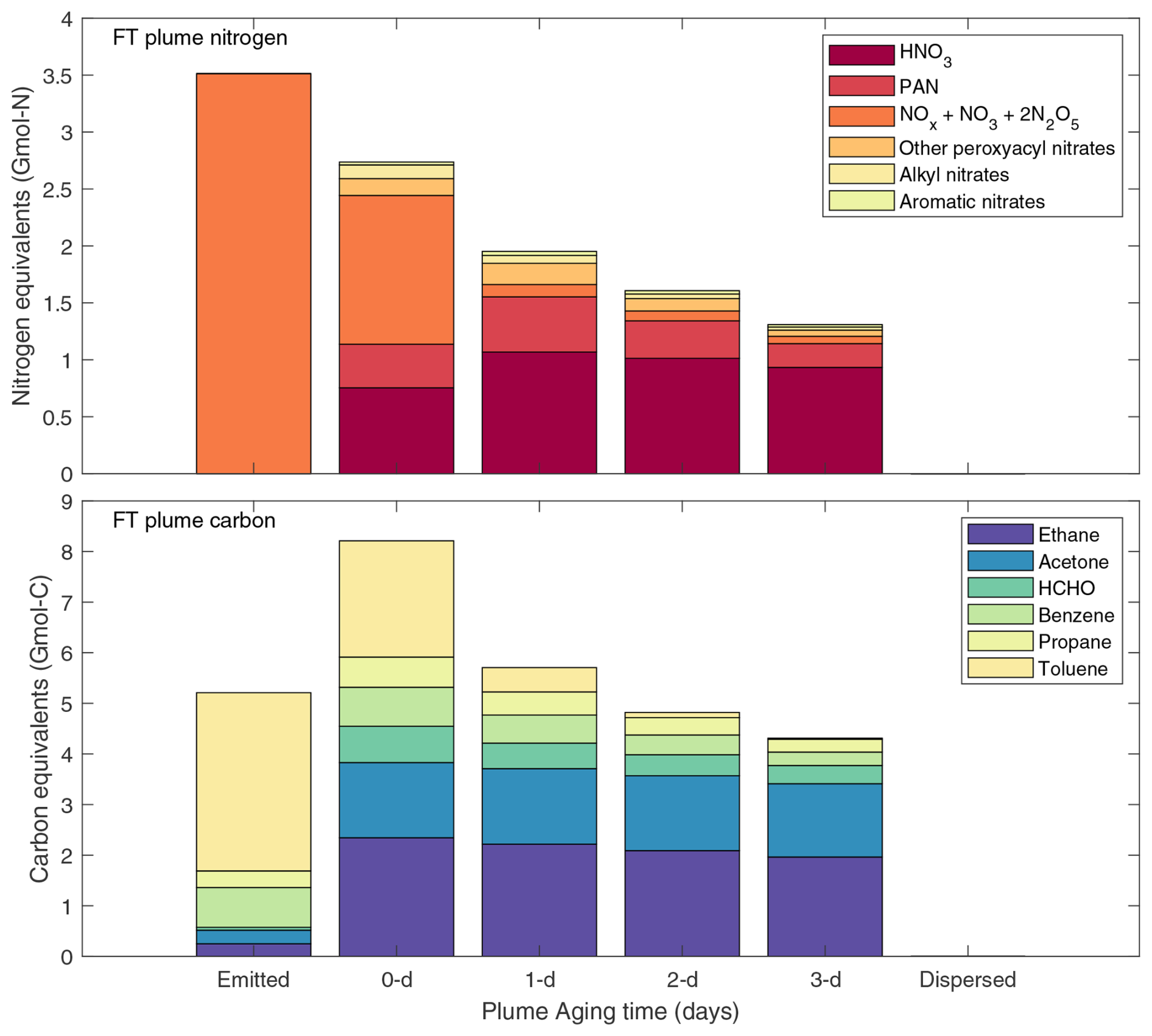
Figure 7 Total NO_y-nitrogen (Gmol-N, top) and VOC-carbon (Gmol-C, bottom) pollution content emitted in the BL-RL stage and aged in the PL stage. “Emitted” designates initial anthropogenic emissions, and “0 d” aging shows the pollution exiting the BL-RL stage, which includes biogenic emissions and background air. Only species with high impact on the O₃ and CH₄ budgets in the DP stage are shown. Loss of total nitrogen occurs through nitrate aerosol formation and gas-phase HNO₃ scavenging. Loss of total carbon occurs through formation of non-plotted secondary VOCs, carbon monoxide, and carbon dioxide. Most ethane in the plume is from background air (i.e., not emitted) which does not impact the budgets.

To provide a reference value for the reactivities in the BL-RL and PL stages, we repeat the PL integrations for control plumes initialized from a control BL-RL run with no anthropogenic emissions (KORUSv5 and GFED5). Subtracting the control run budgets from the standard run budgets yields the budget perturbations induced by South Korean emissions.

3.2.1 Airborne observations

The DC-8 aircraft sampled South Korean pollution on 20 d in May and June 2016, vertically profiling the Seoul Metropolitan Area on most flight days and chasing offshore pollution plumes based on tracer-transport forecasting. We expect the composition of freshly exported plumes from the BL-RL stage to resemble in situ observations in the South Korean BL. In our comparison, we sum observed reactive N species into NO_y-nitrogen in moles of N, specifically NO, NO₂, PAN, and PPN. We do not include other nitrates such as NO₃ and N₂O₅ as they were not individually observed, but measured in combination with HNO₃ and particulate nitrate. Likewise, we sum all VOCs measured at high frequency (1 Hz) into VOC-carbon in moles of C. VOC-carbon includes ethane, benzene, toluene, isoprene, methacrolein, acetaldehyde, acetone, methyl ethyl ketone, methyl vinyl ketone, and formaldehyde, but not CH₄, CO, or CO₂ (KORUS-AQ Science Team, 2019).

Figure 8 shows the 2D histograms of NO_y-nitrogen and VOC-carbon in our model plumes aged 0 and 1 d, and in the observations sampled above and below the BL height, as resolved hourly at 0.25° × 0.25° in the ERA5 data. See Fig. S7 for a map of DC-8 sampling. The dominant plume compositions in the 0 d-aged plumes and BL observations centre on 1.0–3.0 ppb NO_y-nitrogen and 15-25 ppb VOC-carbon, with around +5 ppb more VOC-carbon in the observations. Such a pattern was also observed in transects through Seoul pollution transported west over the Yellow Sea on 22 May. Observations with > 10 ppb NO_y-nitrogen were frequent in the densely sampled Seoul Metropolitan Area and also in fresh urban and industrial plumes off the west (22 May and 05 June) and southeast coast (7, 11, 20, and 30 May); modelled plumes with this range of compositions were also found. After 1 d aging, the modelled plumes had a range of NO_y-nitrogen concentrations resembling FT observations, but with greatly diminished abundances of short-lived aldehydes and alkenes. From this comparison, pollution plumes sampled in the FT, primarily offshore from South Korea, were probably aged less than a day.

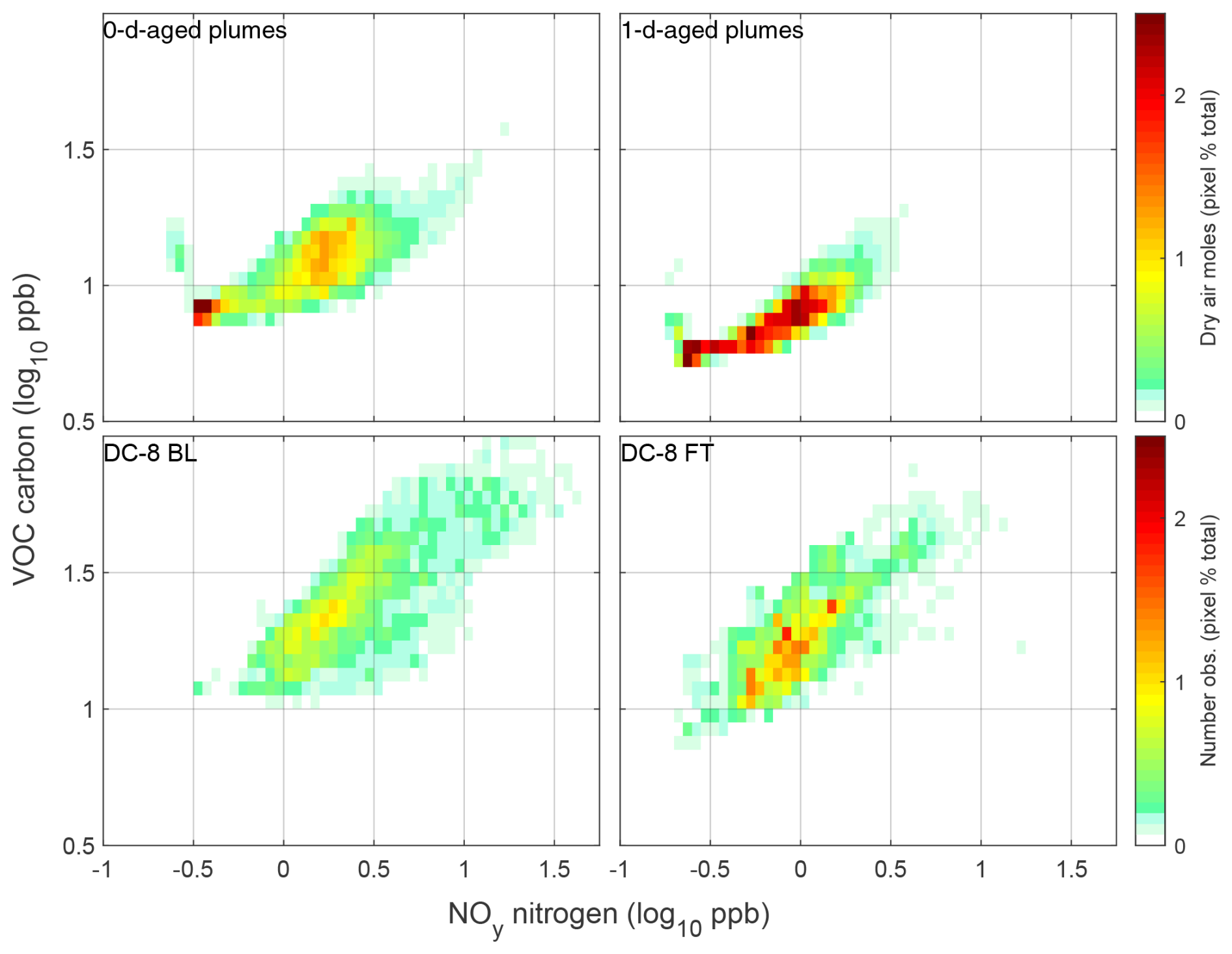
Figure 8 2D distribution of VOC-carbon vs. NO_y-nitrogen in modelled plumes and DC-8 observations. Shown are modelled plumes aged 0 d (top-left) and 1 d (top-right), and DC-8 observations of the BL (bottom right) and FT (top right). Probability densities (colour bar) are normalised total moles (top) and number of observations (bottom) resolved as pixels of 0.05 log₁₀ ppb width. Geographic sampling of DC-8 data is shown in Fig. S7.

3.3 Dispersed pollution (DP) stage

We model the DP stage as a linearly separable chemistry problem. Specifically, we assume that the dispersion of a pollution plume results in a perturbation to the atmospheric chemistry that is sufficiently dilute so that the interaction of two pollutants (i.e., the second-order terms) is negligible. The impact of any pollutant is thus in the linear regime and can be scaled from the integration of a small perturbation. We create a look-up table relating moles of O₃ and CH₄ produced or lost per moles of pollutant X dispersed.

The chemical response of the atmosphere to an added pollutant depends on chemical composition, pressure, temperature, J-values, aerosols, etc. Since we do not model transport in the PL stage, we do not know where the plumes disperse, nor where the remnants are transported afterwards. We choose to disperse the pollutants across four tropospheric layers whose composition is derived from ATom-4 measurements (27 April, 29 April, and 21 May 2018) sampled between 2±1, 4±1, 6±1, and 8±1 km altitude over the northern midlatitude Pacific (see Table 2). At each of the four altitudes we integrate the reactivity of the atmosphere with the addition of 0.1 ppb of pollutant and then subtract a control run made without the added pollutant.

Unfortunately, as the pollutant decays, the background atmosphere also evolves, resulting in a chemical mixture after 30 d that differs greatly from the initial ATom free troposphere. The observed free tropospheric composition is maintained by several non-local processes that are not included in our box model (e.g., lightning NO_x, convective mixing of surface pollution, washout scavenging, injection of stratospheric O₃). Thus, in our F0AM box model we introduce artificial sources or sinks to maintain a stable composition (see Table 6). These artificial terms are derived for the major free-troposphere species at each level with an iterative sequence. First, we fixed the concentrations of the controlled species (NO_x, O₃, CO, H₂O₂, ethane, propane, n-butane, benzene, toluene, acetone) and integrate the full chemistry for 30 d, allowing the numerous short-lived secondary species to achieve some balance. For controlled species with daily net losses, we add an artificial source to match the loss. For those with excess production, we estimate a first-order loss to balance it. Applying these artificial source/sink terms, we run a 365 d constant-summertime spin-up with primary species evolving. We rescale the source/sink terms by the ratio of the initial-to-final concentrations. This process is iterated, with some Aitken acceleration for O₃, until the end-of-year concentrations differ by less than 1 % from the initial ATom values (Table 2). This provides a stable chemical composition upon which to integrate the impact of decaying pollutants.

Table 6 Dispersed plume model parameters and resulting O₃ lifetime.

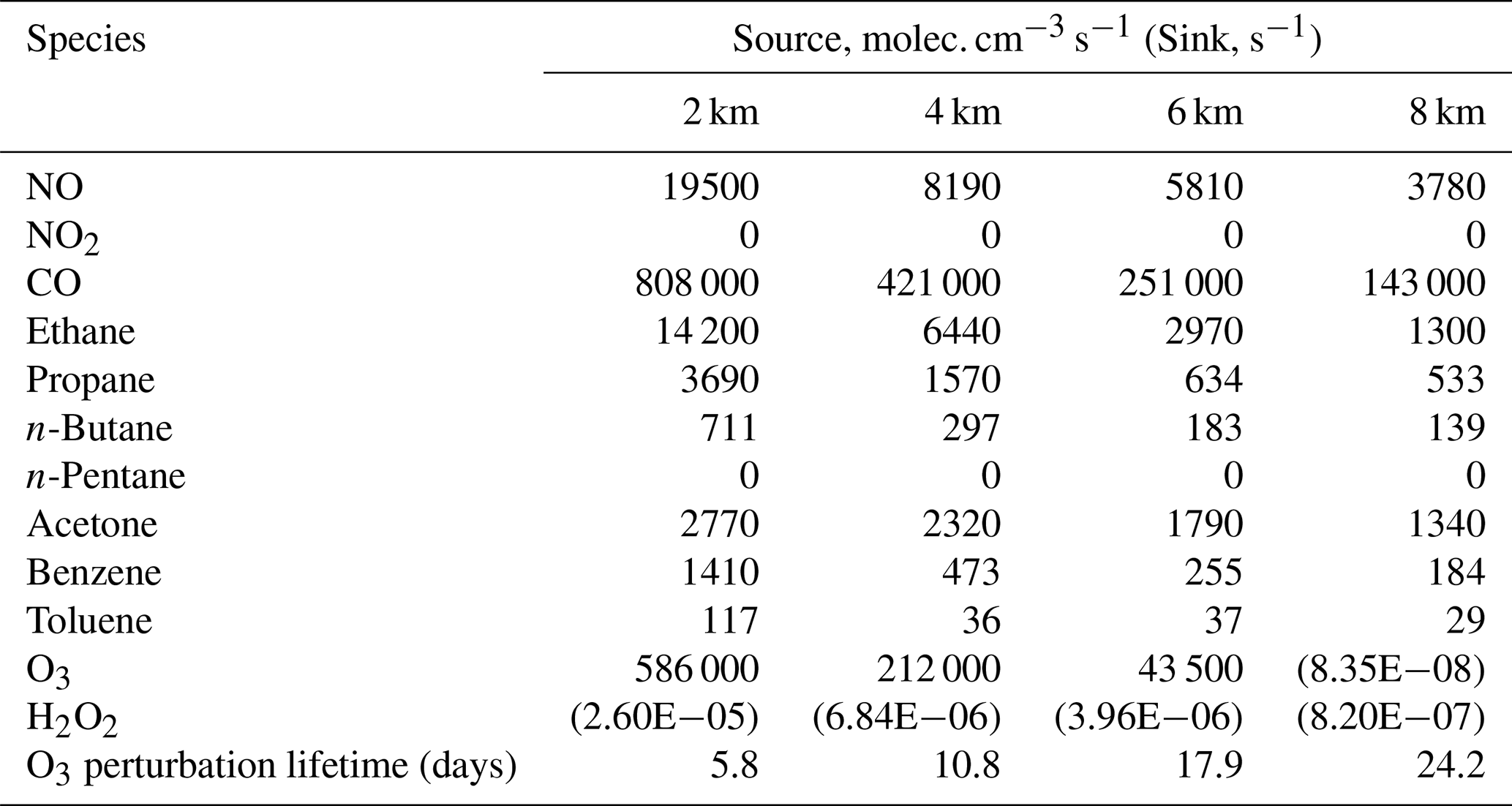
Sources (molec. cm⁻³ s⁻¹) and sinks (s⁻¹) represent the atmospheric processes that maintain a quasi-steady-state for each species for the ATom background atmosphere adopted here. The O₃ lifetimes are derived from the decay of a unit O₃ perturbation at each altitude. Methyl hydroperoxide, which was not constrained in the DP stage, equilibrated at 0.42, 0.30, 0.16, and 0.06 ppb in the altitude bins from 2 to 8 km compared with 0.71, 0.55, 0.40, and 0.23 ppb observed in ATom, consistent with the long-standing view that convection of BL CH₃OOH (not included here) provides a major FT source (Prather and Jacob, 1997).

The DP stage F0AM calculations are integrated as for the PL stage (i.e., constant meteorology, 30 min SZA timestepping, fixed CH₄ and water vapour, and KORUS-AQ all-sky J-values sampled above 1.5 km) for the four altitude bins in Table 2. For each pollutant, we follow the decay of a small enhancement (+0.1 ppb) on the four altitude levels for 30 d. We then collect the remaining moles of pollutant and secondary products (e.g., CO from VOCs) from the four levels, mix them and redistribute again across the four levels (Table 2). This 30 d timescale for mixing is consistent with the vertical age gradients of 3–4 d km⁻¹ found in 3D models (Fig. 9 in Prather, 2025). We repeat this sequence (age 30 d and then mix across levels) three times for 120 d total, effectively oxidizing almost all of the original and secondary pollutants. The vertical mixing is needed to allow the total pollution to decay because the chemical loss of several species is extremely slow if left in the upper troposphere.

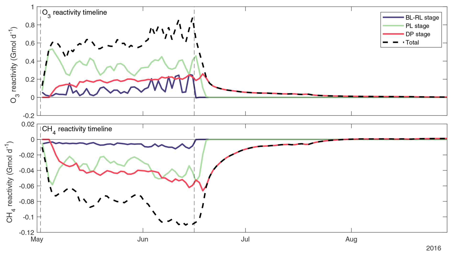
Figure 9 The timeline of O₃ and CH₄ reactivity from 45 d of emissions. The 45 d emission period is enclosed by dashed lines and is followed by a two-day spin-down period. Ozone and CH4 reactivities (Gmol d⁻¹) are shown at daily resolution for the BL-RL stage (blue), PL stage (red), and DP stage (green) and integrate to the model stage budgets in Table 9. The BL-RL reactivities are plotted as daily sums over the model domain for CH4 and over the initial exported plume enhancements for O₃. The PL reactivities are plotted as daily O₃ and CH₄ reactivities in the plumes during aging, synchronised to the timeline according to the plume release times. The DP reactivities are dispersed pollution O₃ and CH₄ changes synchronised to the dispersion of each plume. Daily total reactivities (dashed black line) are the sums of the coloured lines. The spinup of pollution is clear in the first 5 d, and the increasing trends in total reactivities over the next 40 d is driven by the accumulation of DP stage reactivity (green line), and partly by the shift in meteorological conditions in the last 10 d where a longer BL-RL residence time resulted in larger BL-RL reactivities.

For each perturbation by pollutant X, we calculate this 120 d sequence and compare with a reference run made without added pollution. For CH₄ loss (total in ppb), we sum the OH + CH₄ reaction rate for pollution minus control runs. With CH₄ fixed in our model, this directly gives us the pollution-driven net loss. For O₃, the diagnosis of net production is more difficult because the chemistry both produces and destroys O₃ on a time scale of weeks. The use of odd-oxygen production rates to represent O₃ production is fundamentally flawed because these rates depend on the O₃ abundance (see, Guo et al., 2023; Prather and Zhu, 2024). Thus, we use the integral of the O₃ perturbation (ppb days) at each altitude over the 120 d DP integration and divide by the O₃ perturbation lifetime (days) for that altitude. Provided that the O₃ perturbation has fully decayed, this quotient is exactly the net O₃ produced (ppb). For proof, see Prather (2007). The O₃ perturbation lifetime given in Table 6 at each altitude is a well-determined, well-defined value since it is derived from a pulsed O₃ addition and integrated for 120 d (without vertical mixing). With vertical mixing every 30 d, our derivation of net O₃ production is only approximate because we do not follow the perturbation from beginning to end under a single chemistry. For the most part, the O₃ perturbation from pollutant X occurs at the beginning of the 30 d and decays by the end. We do not tabulate the O₃ perturbation caused by an O₃ pollutant since that would be double counting, but we do calculate the CH₄ perturbation caused by O₃.

The O₃ perturbation lifetime at 2 km altitude (5.8 d) is used to calculate the PL stage net production by accounting for the limited decay over 1–3 d. For the DP stage we can simply divide the integrated perturbation (ppb-days) by lifetime (days) to obtain net production (ppb). We rescale these net reactivities by the amount of primary pollutant X used in the calculation to derive dCH₄ $/$ dX and dO₃ $/$ dX in mol mol⁻¹. The total impact of all pollution released to the DP stage (see Fig. 7) is given in Table 7. We find that PAN and peroxypropionyl nitrate (PPN) produce similar dCH₄ $/$ dX and dO₃ $/$ dX reactivity values to NO₂ and NO, and hence we apply the reactivities of NO₂ to all peroxyacyl, alkyl, and aromatic nitrates that we did not calculate explicitly.

Table 7 CH₄ and O₃ budget perturbations in the DP stage from the more important individual pollutants.

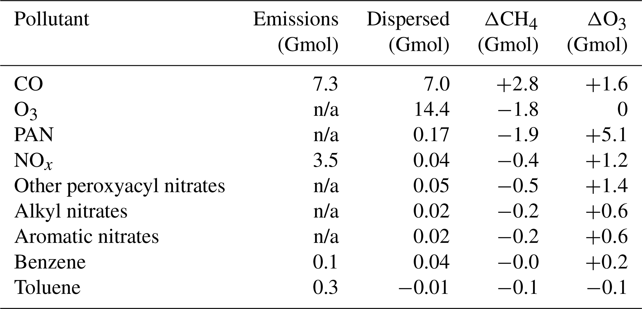
“Emissions” includes 45 d of anthropogenic South Korean emissions (KORUS v5 + GFED5). “Dispersed” values are the pollution remnants after BL-RL processing and 3 d of aging in the PL stage. ΔCH₄ and ΔO₃ are the budget perturbations caused by individual pollutants in the DP stage, and are proportional to the moles of dispersing pollutants. “Dispersed” negative toluene is caused by chemical loss of toluene in entrained FT air that exceeds emissions. n/a = not applicable.

4 Ozone and methane budgets

We calculate the impact of South Korean pollution on O₃ and CH₄ by differencing a full emission run and a reference control run without KORUS v5 anthropogenic and GFED5 biomass burning emissions. Our assessment is for the 45 d of emissions (2 May to 15 June 2016) covering the KORUS-AQ mission in South Korea. We follow 2 spin-down days (16–17 June 2016) without industrial or biomass burning emissions to account for the 45 d of pollution leaving the peninsula. We calculate the budget terms (Gmol) for O₃ and CH₄ directly from all BL, RL, and PL air masses, and then add on DP stage by scaling the dO₃ $/$ dX and dCH₄ $/$ dX factors by the amount of each pollutant X (Gmol) released into the free troposphere.

Following the O₃ budget requires careful accounting. The change in O₃ during the BL-RL stage relative to the control occurs on the order of one day and is almost a direct measure of the net production (loss). Over that time, the net production will decay. The average residence time for dry air in the BL-RL stage is 8 h (mean South Korean BL + RL mass per daily offshore export), but for chemically-produced O₃, it is 12 h. Based on Table 6, we select 4.5 d as the BL-RL O₃ perturbation lifetime at 1 km altitude, and thus, net production of O₃ occurring uniformly across 12 h will decay on average by over 5.4 % by the end of the day. We multiply the BL-RL O₃ perturbation that is put into the PL stage by the reciprocal decay (1.06) to estimate net BL-RL production. The BL-RL stage often produces large net losses from cells with high NO_x emissions, and we assume these perturbations also decay with the 4.5 d timescale. Our method of extracting net BL-RL O₃ production is only approximate because the O₃ perturbation lifetime is likely variable depending on chemical regimes, and the time spent by pollution in the BL-RL stage can vary from hours up to 2 d.

Deriving the net O₃ production from the PL stage is more straightforward. There are three successive 24 h days of plume chemistry integration, occurring under the same atmospheric conditions (2 km) but under different chemical conditions. We do not attempt to derive the O₃ lifetime for each PL case, but make the approximation that it is the same as the free troposphere in the 2 km DP case (5.8 d). At the start of each PL day, we have an O₃ perturbation that is carried forward from the previous day: for day 0 it is the O₃ perturbation from the BL-RL masses that collected in the plume; for days 1-to-3 it is the perturbation at the end of the previous day relative to the control. We assume that this external O₃ perturbation decays with a 5.8 d lifetime (i.e., 16 % d⁻¹). The net internal O₃ perturbation at the end of the day caused by the PL chemistry is then the O₃ at the end of the day minus the decayed residual of the external perturbation from the beginning of the day relative to the control run. Because of decay over the 24 h plume integration, the net internal perturbation is increased by 9 % to get the net production. This complex sequence allows us to account for the effective net O₃ production over the PL stage without double counting. When we integrate the impact of an O₃ perturbation passed on to the DP stage, the integral of CH₄ reactivity is straightforward and must be included, but the integral of the O₃ perturbation itself cannot be included since its net production was already accounted for in the previous stages.

Table 8 Total CH₄ and O₃ budget perturbations and OPE over 45 d of South Korean air pollution.

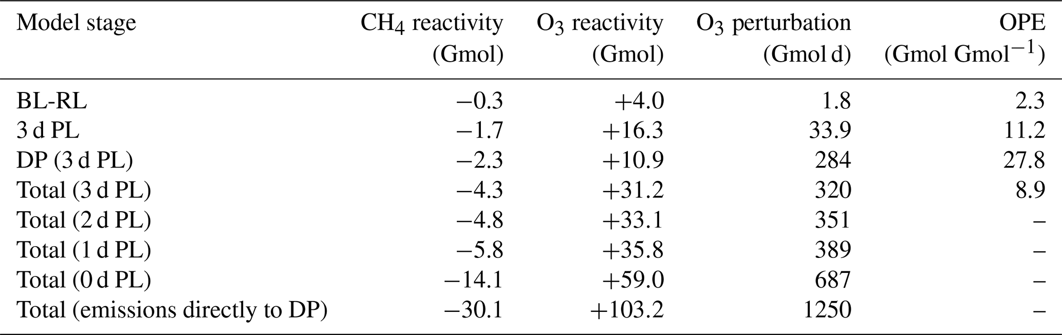
CH₄ and O₃ reactivities are net productions (negative = loss) summed over the individual modelling stages, and as totals for all stages given varying plume aging times. O₃ perturbations are the integrated enhancements of O₃ (Gmol) summed during the stages, and as model totals. Ozone production efficiency (OPE) is computed as the net O₃ production (i.e., “O₃ reactivity”) per NO_y-nitrogen loss (mol mol⁻¹) over several stages, or in total. The DP stage OPE excludes secondary NO_y perturbations from dispersing VOCs.

The total CH₄ and O₃ reactivities attributed to the 45 d of emissions are −4.3 and +31.3 Gmol, respectively, for 3 d plume lifetime (see Table 8). For both species, 85 % of the reactivity occurs during the 45 d emission period, and the remaining 15 % occurs over the following 2 months (see Fig. 9 for reactivity timeline). Table 8 shows the budget terms during the individual model stages, the ozone enhancements that resulted from production, and the ozone production efficiencies (OPE = molar production of O₃ per molar loss of NO_x). Methane and O₃ reactivity occurs mostly in the PL and DP stages, wherein the total budgets are highly responsive to aging time in the plumes (PL stage). Our standard diagnostics are for 3 d plumes, and reducing this lifetime results in much larger reactivities. Varying the plume aging time from 3 to 2 d results in the addition of −0.5 Gmol-CH₄ and +1.9 Gmol-O₃ to the budgets. Varying from 2-to-1 d results in −1.0 Gmol-CH₄, and +2.7 Gmol-O₃, and from 1-to-0 d, −8.3 Gmol-CH₄ and +20.5 Gmol-O₃. The range of reactivities from instant dilution to infinite aging is 11 Gmol-CH₄ and 31 Gmol-O₃ assuming geometric convergence with a common ratio of $\mathrm{1}/\mathrm{2}$. Hence, the change in reactivities from 3-to-2 d aging in plumes accounts for just 5 % of the possible range of reactivities, with 10 % from 2-to-1 d, and 75 % from 1-to-0 d. The true timescales of pollution plume dilution are presently unknown but likely on the order of a few days. Global models commonly dilute pollution plumes too rapidly (Zhuang et al., 2018), and could vastly overestimate the O₃ and CH₄ budget contributions from anthropogenic pollution as a result.

The OPEs in our model stages are diagnosed from the tabulated O₃ production and the loss of reactive nitrogen (NO_x, NO₃, 2N₂O₅, HO₂NO₂, HONO, PAN and other peroxyacyl nitrates, alkyl nitrates, and aromatic nitrates) (not shown). The BL-RL and PL stage OPEs are consistent with Oak et al. (2019) urban South Korean BL OPEs and box modelled DC-8 OPEs that were diagnosed from instantaneous NO₂ formation, odd-oxygen loss, and NO₂-OH oxidation rates. Since half of our NO_x-loss comes from nocturnal N₂O₅ aerosol reactivity, our OPEs are halved compared with Oak et al. (2019). The DP stage OPE diagnosed from pure NO_x dispersion follows the classic non-linear response to NO_x levels (Liu et al., 1987) and is close to the OPE from aviation NO_x (31 mol mol⁻¹; Prather and Zhu, 2024).

5 Conclusions

Our modelling system calculates the tropospheric OH-loss of CH₄ and the net production of O₃ from South Korean air pollution during the May-June 2016 KORUS-AQ period. Methane loss is diagnosed from CH₄+OH rate in all three modelling stages, from boundary layer to plumes to the ultimate dispersion in the free troposphere. Ozone production is inferred through the integrated O₃ perturbation (i.e., mole-days) and our calculation of the O₃ perturbation lifetimes (i.e., days). This use of a perturbation lifetime to derive the effective “emission” of O₃ is necessary because the typical modelling approach of using the odd-oxygen rates (e.g., Griffiths et al., 2021) fails to account for the feedbacks of O₃ on the production of odd-oxygen as discussed in Prather and Zhu (2024).

The total perturbations to CH₄ and O₃ caused by 45 d of South Korean air pollution are −4.3 and +31.3 Gmol respectively. The global annual tropospheric CH₄ loss for this period is about 35 200 Gmol (Saunois et al., 2025), and hence the 45 d global loss is 4300 Gmol. The tropospheric O₃ budget is more complex than the CH₄ budget, but if we take a simple estimate from the models reporting odd-oxygen rates in Griffiths et al. (2021), we have a mean tropospheric burden of 7020 Gmol (337 Tg-O₃) and a production time of 27 d. Thus, the global reactivity for the 45 d KORUS period is −4300 Gmol CH₄ and +11 700 Gmol O₃. We estimate the South Korean NO_x emissions to be of order 1 % of global anthropogenic emissions (Hoesly et al., 2018), and scaling this gives 10 % of total CH₄ loss and 27 % of total O₃ production attributable to anthropogenic pollution. Our scaling estimates are simplistic and biased high because the reactivity of pollution depends greatly on latitude and season. The KORUS-AQ campaign was during a period of greatest photochemical activity. Unfortunately, we do not have the data sets and capability to repeat this study with the full annual cycle of Korean pollution.

The O₃ and CH₄ reactivities are highly sensitive to the aging of pollution in plumes. If the plumes disperse to the free troposphere immediately (0 d PL in Table 9), the total reactivities approximately double our standard estimates for 3 d aging. Typically, global models fail to preserve interior plume concentrations beyond a few days at best due to numerical diffusion (Zhuang et al., 2018). The inability to maintain pollution in large-scale plumes is probably one of the larger sources of error in CTMs, and the community would benefit from observational studies on pollution plume dynamics to establish the typical timescales of mixing into the free troposphere. Atmospheric chemistry MIPs could incorporate our results by performing a regional air quality CTM study, e.g. for South Korea, and comparing the resulting CH₄-OH loss and O₃ mass perturbations. Diagnosing O₃ production from the mass perturbations, as done in this work using lifetimes, remains a challenge.