Sorting sudden stratospheric warmings with the downward tropospheric influence using ERA5 and CESM2-WACCM

Sudden Stratospheric Warming events (SSWs) can have a downward impact on the troposphere, but the mechanism remains uncertain. This study focuses on classifying SSWs based on their tropospheric responses and documenting associated dynamical characteristics. Using the ERA5 data and CESM2-WACCM outputs, 52 SSWs are identified in ERA5 and 273 in CESM2-WACCM, with 33 and 119 downward-propagating SSWs (DWs), respectively. The DWs are classified into three types based on cold surges over Eurasia (EA), North America (NA), and both (BOTH), respectively. Both DWs and non-downward-propagating SSWs (NDWs) weaken and deform the polar vortex, but DWs induce stronger negative Northern Annular Mode (NAM) and North Atlantic Oscillation (NAO) responses. For DWs, the anomalous high develops in the polar region, which deflects to lower latitudes, consistent with the frequent appearance of the polar high and the midlatitude blockings. The shape of the anomalous polar high varies with the DW type, and the extension and shift of the anomalous high lead to different surface responses. The DWs are also accompanied by a southward shift of the precipitation belt, especially over the oceanic and coastal regions. The relatively weaker tropospheric impact of NDWs may be partly explained by their weaker stratospheric disturbance amplitude. The three types of DWs differ in spatiotemporal evolutions of the NAM and NAO pattern, different forcing by planetary waves, and varying ratios between displacement and split. This study reveals the diversity of the DWs and distinguishes their potential impacts on both continents in the Northern Hemisphere.

1 Introduction

In the northern winter stratosphere, the polar temperature increases dramatically in just a few days when the polar vortex deforms or even collapses, and meanwhile the circumpolar westerly winds decrease suddenly and even reverse the direction (Baldwin et al., 2021). This phenomenon, known as sudden stratospheric warming (SSW), is an important manifestation of stratosphere–troposphere coupling in spring and winter. The SSW occurrence is associated with strong, upward-propagating planetary waves from the troposphere (Sjoberg and Birner, 2012; Butler et al., 2015). Recent studies also found that stratospheric preconditioning might play a decisive role in inducing the SSW event, by determining the intensity of the interaction between planetary waves and the mean flow (White et al., 2019; Yang et al., 2023). Polvani and Waugh (2004) suggested that SSWs are caused by a sharp increase in the amplitude of planetary-scale waves (primarily wave 1 and 2) propagating upward from the troposphere and perturbing the stratospheric polar vortex. Modeling evidence shows that the wave 1 forces the displacement of the polar vortex from the North Pole (Lindgren and Sheshadri, 2020), while the wave 2 determines the extent of vortex elongation and deformation (Baldwin et al., 2021).

Stratospheric variability associated with SSWs affects the near surface weather and climate through stratosphere–troposphere coupling processes (Hitchcock and Simpson, 2014; Wu and Reichler, 2019). Several mechanisms have been proposed to explain the possible downward impact of the stratosphere on the troposphere, including wave-flow interaction theory (Kuroda and Kodera, 1999), balanced flow dynamics theory (Black, 2002; Haynes et al., 1991), planetary wave refraction theory (Schmitz and Grieger, 1980), non-local potential vorticity response (Ambaum and Hoskins, 2002), and isentropic atmospheric meridional mass circulation theory (Cai and Shin, 2014). The wave-mean flow interaction theory suggests that upward-propagating tropospheric wave forcing fluctuations affect stratospheric mean flows, which in turn affect the vertical propagation of planetary waves (Kuroda and Kodera, 1999; Hartmann, 2000). As a consequence, the stratospheric disturbances cause significant downward impact on tropospheric circulation variations and near surface climate anomalies (Colucci and Kelleher, 2015; Dall'Amico et al., 2010), which are proposed to be amplified by tropospheric eddy feedback (Kidston et al., 2015).

SSWs can have a considerable impact on the troposphere and a sustained effect on surface weather for weeks or even months (Domeisen et al., 2020; Rao et al., 2021; Lu et al., 2023). The weakened polar vortex during SSW usually projects onto the negative phase of the Northern Annular Mode (NAM) and/or the North Atlantic Oscillation (NAO), which gradually propagates downward (Karpechko et al., 2017; Kunz and Greatbatch, 2013; White et al., 2019). The negative phase of the NAM is often accompanied by equatorward shifts in storm paths and tropospheric jets (Kidston et al., 2015), shifts in the centre of the East Asian jets, variation in the blocking frequency (Anstey et al., 2013), increased possibility of cold air outbreaks over Eurasia and North America (Baldwin and Dunkerton, 2001; Lehtonen and Karpechko, 2016; Lu et al., 2022; Yan et al., 2022), and likelihood of extreme rainfall (Karpechko and Manzini, 2012).

The common characteristics of SSWs have been widely reported in literature (see Baldwin et al., 2021 and references therein). However, every SSW has its individual features and displays strong particularity (Karpekho et al., 2017; Rao et al., 2018, 2019, 2021; Lu et al., 2023). It is the differences between individual SSWs and the background conditions that distinguish their influence on the troposphere. Accordingly, the tropospheric signals exhibit substantial differences in their extent, spatial coverage, and overall structure. Possible factors explaining the SSW individuality especially in its influence include the SSW strength, the initial warming location or the warming center (Zhang and Chen, 2019; Yan et al., 2022), the warming duration time (Hitchcock and Simpson, 2014), details of the wave flux between the troposphere and stratosphere (Shi et al., 2024), and the geometry of the polar vortex (split or displacement) (Maycock and Hitchcock, 2015; Rao et al., 2020). Therefore, the SSWs can be classified into different types based on those metrics.

Different SSW classifications are widely used in literature. For example, based on vortex geometry shape the SSWs are classified as split, displacement, and mixed types (Charlton and Polvani, 2007; Rao et al., 2019). Based on whether the stratosphere reflects planetary waves during the westerly recovery phase following the SSW onset, it can be divided into absorbing and reflecting types (Kodera et al., 2016). According to whether the event has had a significant impact on the troposphere, it can be grouped into downward (DW) or non-downward (NDW) types (Jucker, 2016; Runde et al., 2016; Karpechko et al., 2017; White et al., 2019; Chwat et al., 2022). Although the DW SSWs show negative NAM signals from the troposphere to the stratosphere, the near surface response structure is still different among DWs, with cold extreme sometimes only appearing in Eurasia, sometimes only in North America, and sometimes in both continents. However, there is still not a widely accepted subclassification for DWs events based on the coverage of the near-surface cold anomalies associated with SSW. This study is mainly concerned with two questions: (1) What are the inter-case differences in the DW influence on the troposphere although by definition the NAM during DWs shows downward propagation to the lower troposphere? (2) What can we learn from the classification for DWs? While the present analysis does not aim to establish a direct causal mechanism for these differences, it highlights robust and systematic contrasts among DW events. This identification provides a physically interpretable framework for organizing the diversity of DW events and offers useful information that may help constrain and guide future investigations into the mechanisms governing their tropospheric impacts.

The primary objective of this paper is to classify SSWs based on their tropospheric responses and to document the associated dynamical characteristics. The organization of the paper is constructed as follows. Following the introduction, Sect. 2 describes the data and methods used in this paper. Section 3 compares the tropospheric response characteristics of various DW events. Section 4 analyzes the dynamics related to various DW events. Finally, Sect. 5 provides a summary and discussion.

2 Data and methods

2.1 Reanalysis data

We use the European Centre for Medium-Range Weather Forecasts (ECMWF) fifth generation reanalysis (ERA5) dataset over the period from October 1940 to December 2022. The data prior to 1958 are used with an expectation of selecting more SSW samples. Both three-dimensional and two-dimensional data are used. The three-dimensional variables on the isobaric levels include the air temperature, the geopotential, the zonal and meridional winds, and the vertical velocity on p coordinate. The two-dimensional variables at a single surface level include total precipitation and the temperature at 2 m (t2m). The isobaric levels extend from 1000 to 1 hPa, and the local horizontal resolution of the ERA5 is 0.25° latitude by 0.25° longitude (this dataset is collected at 1.5° latitude by 1.5° longitude for easy handling).

2.2 Model data

Considering that the SSW samples from the ERA5 reanalysis are not too large, three historical simulations (r1i1p1f1, r2i1p1f1, and r3i1p1f1) from the CESM2-WACCM are employed to increase the SSW number. The CESM2-WACCM model has been shown to simulate the SSW frequency, displacement versus split types, and the downward impact well (e.g., Liang et al., 2022). The historical simulation starts from 1850 and ends in 2014, which is one of the common experiments from CMIP6. Daily outputs from CESM2-WACCM have a horizontal resolution of 0.9° latitude by 1.25° longitude at 8 standard pressure levels from 1000 to 10 hPa.

The daily climatology is computed as the long-term mean for each calendar day, and the raw daily climatology is smoothed using 31 d means. The daily anomalies refer to the detrended deviation relative to the smoothed daily climatology.

By examining the same classification framework in both ERA5 and CESM2-WACCM, this study aims to assess whether the identified SSW type distinctions are reproducible across different data sources, rather than being dependent on a specific reanalysis product.

2.3 DW and NDW event definitions

We use the definition from Charlton and Polvani (2007) to identify SSWs in the Northern Hemisphere. Specifically, all days when a change in the zonal-mean zonal wind $\stackrel{\mathrm{‾}}{u}$ from westerlies to easterlies occurs at 60° N and 10 hPa within the period from 1 November to 31 March each year are selected. The first day when $\stackrel{\mathrm{‾}}{u}$ undergoes a transition from westerlies to easterlies is defined as the onset date of this SSW. Several SSW definitions considering the wind reversal at different latitudes and heights in the circumpolar region have been compared by Butler and Gerber (2018). They concluded that a small modification in the wind position or the wind threshold used for the SSW definition does not lead to major changes in the statistics of the SSWs. Considering the zonal winds change radically even after the SSW onset, the onset date of the two SSW events must be more than 20 d of consecutive westerlies apart (roughly double the radiative timescales in the middle stratosphere). Further, $\stackrel{\mathrm{‾}}{u}$ must have recovered to westerlies at least for 10 consecutive days prior to 30 April, which can exclude final warmings (e.g., Charlton and Polvani, 2007). Finally, 52 SSWs are selected from ERA5, and 273 SSWs are selected from CESM2-WACCM. The average occurrence frequency of SSW is approximately 0.63 per year in ERA5 and 0.55 per year in CESM2-WACCM, consistent with previous studies (Liu et al., 2019; Rao and Garfinkel, 2021).

To classify the SSW as the DW or the NDW, the NAM index is calculated (Baldwin and Thompson, 2009). After removing the daily climatological mean from the geopotential heights, the anomaly data are area-weighted (i.e., multiplied by cosine of the latitude) over 20–90° N. The anomaly data are normalized for each pressure level, and the empirical orthogonal function is performed to extract the leading mode (i.e., the NAM pattern). The anomaly field is projected onto the leading mode to compute the corresponding time series (i.e., the NAM index). After the NAM index is obtained at each pressure level, the index at 1000 hPa is used to represent the NAO index. The NAM index for each pressure level is calculated separately, and the NAM at 150 and 850 hPa is used to identify DWs.

The definition of DWs used in this paper follows the method by Karpechko et al. (2017). Namely, a DW is defined when the SSW satisfies the following three conditions: During the 45 d period from day 8 to day 52 relative to the SSW onset date, (1) the average NAM index is negative at both 1000 and 150 hPa; (2) the percentage of days with a negative NAM index is greater than 70 % at 150 hPa; and (3) the percentage of days with a negative NAM index is greater than 50 % at 1000 hPa. To reduce the effect of topographic complexity over high-terrain regions, White et al. (2019) adjusted 1000 hPa to 850 hPa for the first and third conditions, which are also adjusted in this study. Based on these criteria, 33 DWs (63 % of all SSWs) are identified in ERA5, compared to 119 DWs (44 % of all SSWs) from CESM2-WACCM.

2.4 Classification of DWs

It is assumed that following the DW event onset, continental cold anomalies can develop over Eurasia and/or North America, implying an increase in cold air outbreaks after the DW SSW onset. To better describe and distinguish the DWs, we further divide DWs based on the near-surface (2 m) air temperature anomalies over land within 40 d after the onset of DWs. Considering that cold surges are more active over the Eurasia (Europe + Asia) and North America (US + Canada) following the DWs, a comparison between the cold anomalies over the two regions can further classify the DWs into three types: cold anomalies only appearing over North America (NA), only appearing over Eurasia (EA), and over both regions (BOTH). Regions focused in this study include Europe (40–70° N, 0–60° E), Asia (40–70° N, 60–140° E), United States (30–46° N, 70–120° W), and Canada (46–60° N, 60–120° W). Within one region, the area-averaged 2 m temperature anomalies over a 40 d period are considered to be associated with the downward impact of the DW if the anomalies meet the following two criteria: (1) the percentage of days with cold anomalies is greater than 50 %; (2) the mean temperature anomaly over a 40 d period is less than −0.3 °C. This threshold can classify all DWs into the three types. For the mainland, as long as one district meets the criteria, it is considered to be associated with the downward impact of the preexisting DW.

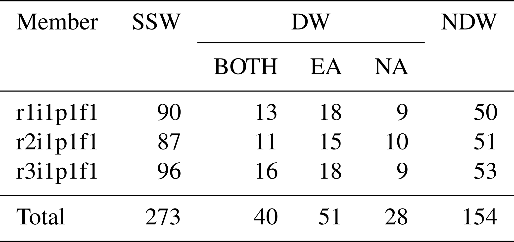
The classification of SSWs into split and displacement events is based on the method initially developed by Mitchell et al. (2011) and adapted by Seviour et al. (2013) using the two-dimensional (2D) moment analysis method. Maycock and Hitchcock (2015) modified this analysis method by using the geopotential height at 10 hPa instead of the potential vorticity used in Mitchell et al. (2011). Maycock and Hitchcock (2015) defined the edge of the polar vortex as the climatological mean geopotential height over 60° N and 10 hPa in winter, and this definition is adopted in this study. Maycock and Hitchcock (2015) employed the following thresholds: a displacement event is identified when the centroid latitude is less than 66.5° N for a minimum of seven consecutive days, while a split event is defined when the vortex aspect ratio larger than 2.8 for at least seven consecutive days. Several modifications for some parameters in this study are as follows. We choose the thresholds as the most equatorward 5.7 % of centroid latitudes and largest 5.2 % of aspect ratios, yielding a threshold of 62.9° N for centroid latitude and 2.46 for aspect ratio, respectively (e.g., Mitchell et al., 2011; Seviour et al., 2013). Table 1 shows the onset date and specific categorization of each event in ERA5. The general statistics of SSWs from the three historical simulation members by CESM2-WACCM are shown in Table 2. In ERA5, types BOTH, EA, NA and NDW account for approximately 25 %, 27 %, 12 % and 36 % respectively. In CESM2-WACCM, the corresponding proportions are 14 %, 19 %, 11 % and 56 %, respectively.

Table 1 Statistics of the SSWs from 1940–2022. The second column (S/D) shows the SSW type based on the vortex shape (D = displacement, S = split). The third column shows the SSW type based on whether the stratospheric signal propagates downward (DW = downward, NDW = non-downward). The last column shows the subclassification of DWs.

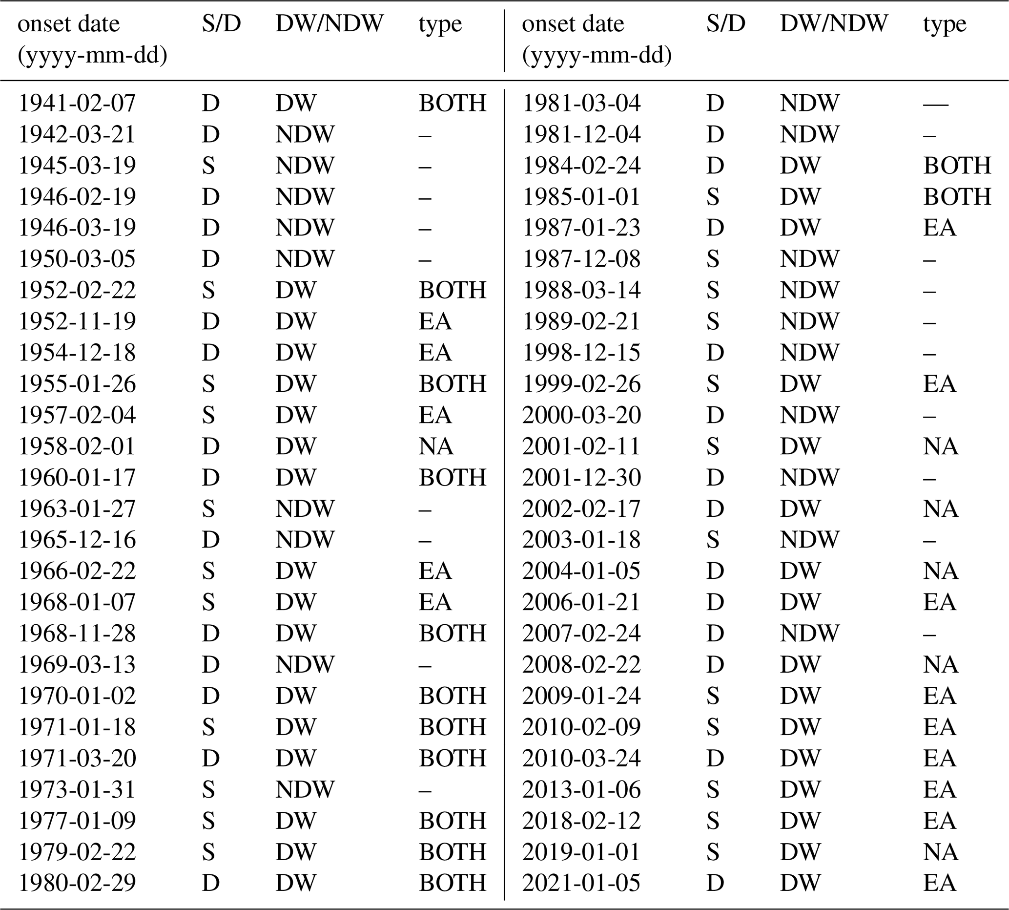
Table 2 General statistics of SSWs from the three historical simulation members by CESM2-WACCM.

2.5 Isentropic potential vorticity

In this paper, isentropic potential vorticity (IPV) is used. The vertical component of IPV is defined (Hoskins et al., 1985) as:

$$\begin{array}{}\text{(1)}& \text{IPV}=-{\displaystyle \frac{g\left(f+\mathit{k}\cdot {\mathrm{\nabla }}_{\mathit{\theta }}\times \mathit{V}\right)}{\frac{\partial p}{\partial \mathit{\theta }}}},\end{array}$$

where f is the Coriolis parameter, θ is the potential temperature, g is gravity acceleration, p is air pressure, k is the vertical unit vector, and V is horizontal wind vector at isentropic surface.

2.6 Eliassen–Palm (E–P) flux

The E–P flux and its divergence can characterize the propagation of quasi-geostrophic planetary waves and its interaction with the mean flows. The E–P flux and its divergence are employed to diagnose the dynamical processes during SSWs as follows (Edmon et al., 1980):

$$\begin{array}{}\text{(2)}& {\displaystyle }{F}_{\mathit{\phi }}=-a\left(\cos \mathit{\phi }\right)\stackrel{\mathrm{‾}}{u{}^{\prime }v{}^{\prime }},\text{(3)}& {\displaystyle }{F}_p=a\left(\cos \mathit{\phi }\right)f{\displaystyle \frac{\stackrel{\mathrm{‾}}{v{}^{\prime }\mathit{\theta }{}^{\prime }}}{\stackrel{\mathrm{‾}}{{\mathit{\theta }}_p}}},\text{(4)}& {\displaystyle }\mathrm{\nabla }\cdot \mathit{F}={\displaystyle \frac{\mathrm{1}}{a\cos \mathit{\phi }}}{\displaystyle \frac{\partial \left(F_{\mathit{\phi }}\cos \mathit{\phi }\right)}{\partial \mathit{\phi }}}+{\displaystyle \frac{\partial F_p}{\partial p}},\end{array}$$

where F_φ is the horizontal component of the E–P flux, F_p is the vertical component, and ∇⋅F is the divergence of the E–P flux, and a, φ are the Earth's radius and latitude, respectively. The E–P flux vector characterizes the propagation direction of the planetary waves. The E–P flux divergence indicates the effect of the planetary waves on the mean flow. When the E–P flux is convergent (divergent), it indicates that there is easterly (westerly) forcing of the mean flow.

3 Comparison of tropospheric responses to three types of DWs

3.1 Spatiotemporal evolution of the NAM

The NAM index can be used to characterize the downward propagation of stratospheric disturbance. The composite evolutions of the NAM index for the three types of DWs are compared in Fig. 1. Consistent with previous study (Karpechko et al., 2017; Kunz and Greatbatch, 2013; White et al., 2019), negative NAM signals appear above 200 hPa within a few days around the SSW onset date. After the DW onset, the negative signal propagates downward into the troposphere (Fig. 1a1–c1), forming a typical dripping-paint pattern in the troposphere (e.g., Baldwin and Dunkerton, 2001). On day 20 and afterward, the upper stratosphere gradually recovers to the positive NAM, while the negative signal below 50 hPa returns to the positive NAM at different times for the three types of DWs. The negative NAM signal below 50 hPa can persist until day 60 and even afterward, suggesting that the downward influence of DWs is persistent, which is consistent with previous suggestions of enhanced tropospheric predictability following SSWs (Rao et al., 2021; Lu et al., 2023). Differences in the NAM evolutions are noticed for the three types of DWs in ERA5.

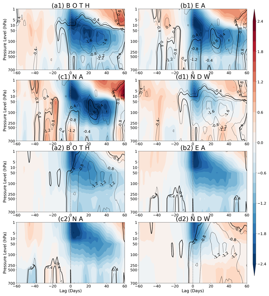
Figure 1 The composite evolution of the NAM index for (a–c) three types of DWs and (d) NDW events. (a) BOTH, (b) EA, (c) NA, (d) NDW. The reanalysis is numbered with “1” following the plot letters, and the model simulation is numbered with “2”. The units are in standard deviations. The dashed contours represent the difference between (a) BOTH and NDW (BOTH − NDW), (b) EA and NA (EA − NA), the contours show. The black line represents statistical significance at the 95 % level for the difference (contours).

1. In the pre-SSW onset period, the NAM displays different behaviors. The positive NAM mainly develops around day −50 and day −30 with the most significant signals in the lower stratosphere and upper troposphere for the type BOTH. The positive NAM only develops in the upper stratosphere around day −30 for the type EA. In contrast, type NA exhibits characteristics markedly distinct from other types: the positive NAM dramatically develops from day −50 in the upper stratosphere to day −15 in the lower troposphere, forming a pronounced vertical structure extending from the upper stratosphere to the lower troposphere (Fig. 1c1).

2. In the post-SSW onset period, the negative NAM is structured in different spatiotemporal dripping shapes. Around 20 d or more after the SSW onset, the NAM is reversed in the upper stratosphere, while the reversion time in lower levels is later. The negative NAM at 50 hPa persists longer than any other level for all types of DWs and even NDW. In contrast, the NAM sign reversion is earliest for NA out of the three DW types around day 50 at 50 hPa (Fig. 1c1), while the NAM sign change is much slower for BOTH and EA beyond day 60 (Fig. 1a1 and b1). It is also seen that the NAM sign change for NDW is also around day 50 at 50 hPa (Fig. 1d1).

3. The process of converting positive NAM to negative NAM exhibits relatively minor differences for the DWs and NDW. The NAM evolves from moderately positive to moderately negative for the type BOTH. It evolves from weakly positive to weakly but persistently negative for type EA in ERA5, and this signal transition is not significant in the model. Further, it evolves from intensely positive to intensely but shortly negative for type NA. The strong phase transition for NA in ERA5 may be due to the small sample size and the influence of individual cases.

4. The near surface exhibits different behaviors in the NAM intermittent signals for the three types of DWs. Specifically, the negative NAM at the near surface is continuous for BOTH and EA types, while it is very short in the persistent time and shows a low significance level for NA. At the very beginning of the NA DWs, the NAM is still positive at the near surface due to the lagged downward impact of the stratosphere, with the negative NAM from day 10 to day 50. In contrast, the negative NAM signal fails to appear at the near surface for NDWs, only with significant positive NAM around day 30. The difference between BOTH and NDW and between NA and EA is most significant in the troposphere and near surface, implying a diversity in the persistency and NAM intensity among SSW types.

Comparing CESM2-WACCM simulations (Fig. 1a2–d2) with ERA5, the pre-SSW signals are not clearly discernible in CESM2-WACCM, yet the characteristics of the NAM is highly consistent. The conclusions are nearly unchanged if the reanalysis is replaced by model simulations: the downward propagation of the NAM is more continuous during EA than NA, and the NAM is much shallower during the NDW than during DWs. The similar evolution patterns observed in ERA5 and CESM2-WACCM indicate that the characteristic differences are not confined to the fewer events in the observational data, lending confidence to the robustness of the conclusions.

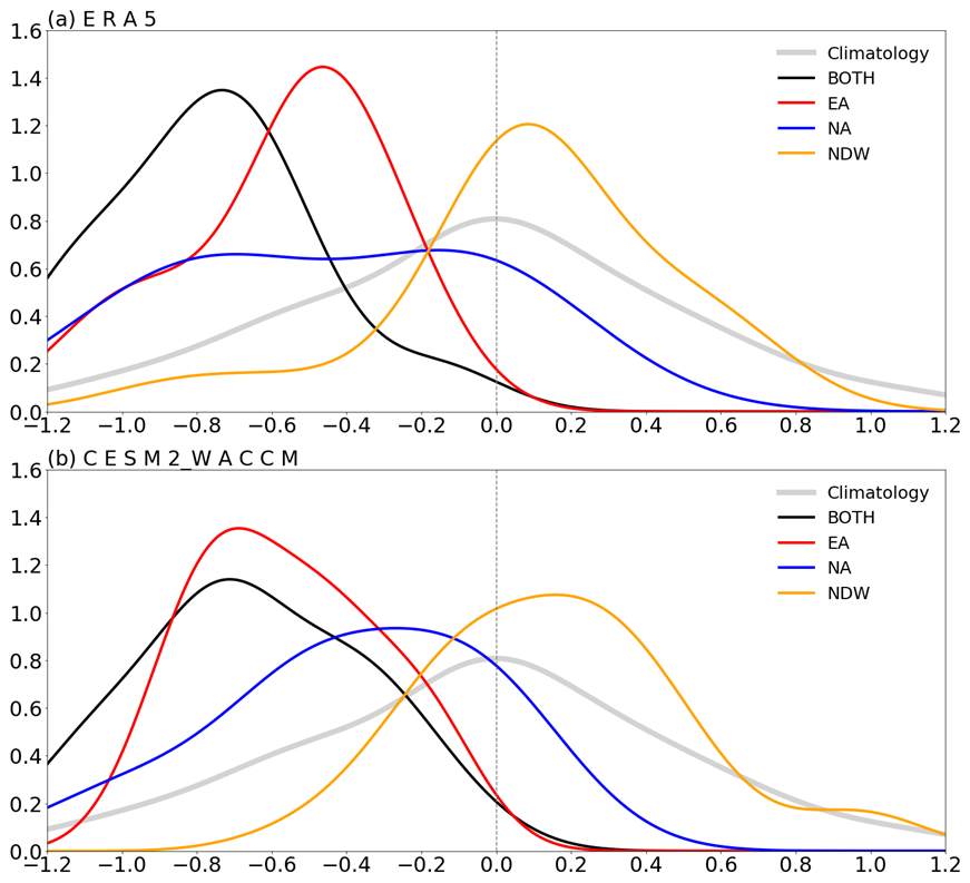
Figure 2 Probability density functions for the average NAO index during the 60 d after SSW onset date for BOTH (black curve), EA (red curve), NA (blue curve), and NDW (orange curve) events from two datasets: (a) ERA5 and (b) historical simulations by CESM2-WACCM. The climatological distribution (grey curve) is constructed from a combined sample of 2000 randomly selected 60 d winter periods drawn from both ERA5 and CESM2-WACCM. The Kernel Density Estimation is used for the 60 d mean index to smooth the PDF curve.

The NAO index is closely related to low-level circulation over the North Atlantic, which is significantly correlated with the probability of extremes, such as regional coldness, snowstorm, and strong winds (Thompson and Wallace, 2001; Scaife et al., 2014). Figure 2 compares the probability density functions (PDFs) of the 60 d average NAO index after the onset for each type of event. Comparisons with a random sample of 2000 winters show that the probability distribution of the NAO index for DWs shifts left toward negative, which indicates that DWs have a significant effect on the surface circulation by projecting onto more negative NAO. In ERA5 (Fig. 2a), the NAO index after the DW onset for BOTH is 2–3 times more likely to be less than −0.8 than for other cases, with the median roughly located at −0.7, and the probability that the index is positive is almost zero. The median values of the NAO after EA and NA are the same, roughly located at −0.5, but the difference is noticeable. Namely, the PDF of the NAO for NA is more dispersed and the PDF peak is smaller than that for EA and BOTH. In contrast, the type BOTH showed the largest composite mean of NAO (−0.762), followed by EA (mean NAO $=-\mathrm{0.567}$) and NA (mean NAO $=-\mathrm{0.435}$). The PDF of NAO for NDW is primarily concentrated between −0.2 and 0.4 (68.4 %), with median and mean values near 0.1 and 0.088, which might indicate that the NAO nearly has no preference during NDW events.

In the model simulation (Fig. 2b), the probability density function distribution of the NAO indices also highly resembles that in ERA5 (Fig. 2a). Namely, the mean probability density function for BOTH and EA is much more left-skewed than that for NA. Consistent with ERA5, the probability density functions of BOTH and EA exhibit a higher degree of overlap. The probability density function for NA is distributed more flattened than that for BOTH and EA. Moreover, due to the larger sample size, the peak values can be seen more clearly for NA. The probability density function distribution is almost symmetric on both sides of zero for NDW in both ERA5 and CESM2-WACCM, although the peak value (∼1.1) is larger than that for the climatological probability density function (∼0.8).

3.2 Comparison of near surface response

Due to the definitions of the SSW types, the near-surface temperature impacts exhibit marked differences naturally. Figure 3 shows the composite t2m anomalies and their differences in the 40 d intervals before and after the SSW onset visually. Specifically, in the pre-SSW period (day −40 to day 0), significant cold anomalies have well developed over northern Eurasia for BOTH and EA, while the cold anomalies are not detectable over Eurasia for NA (Fig. 3a–c). Although cold anomalies also appear over Eurasia, the anomaly magnitude is fairly weak for NDWs (Fig. 3d). The western coast of North America is covered with cold anomalies for BOTH and NDW (Fig. 3a and d), while significant warm anomalies appear over most of North America for EA and NA (Fig. 3b and c). It is also found that significant warm anomalies develop over Europe for NA (Fig. 3c). For BOTH and EA, an anomalous high appears over the Arctic at 500 hPa, while for NA two anomalous high centers appear over North America and Europe, respectively (Fig. 3a–c). The tropospheric circulation anomalies are much weaker for NDWs than DWs (Fig. 3d). The general patterns of t2m and 500 hPa height anomalies are highly consistent between ERA5 and CESM2-WACCM simulations. In the post-SSW period, the t2m anomaly patterns differ among the DW types and the NDW, consistent with the surface-temperature-based definition of the events. DW events exhibit cold anomalies over their respective defining regions, while NDW events lack coherent surface temperature signals. These characteristics are similarly represented in ERA5 and CESM2-WACCM.

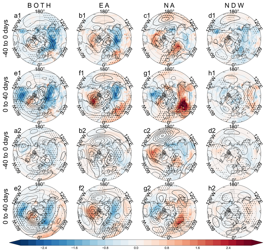
Figure 3 Composite 2 m temperature (t2m) anomalies (shadings; units: K) and 500 hPa geopotential height anomalies (contours; units: gpm) for (a, e) BOTH, (b, f) EA, (c, g) NA and (d, h) NDW events before the SSW onset (top row) and afterward (bottom row) from two datasets: (a1–h1) ERA5 and (a2–h2) historical simulations by CESM2-WACCM. The composite is based on the mean of 40 d intervals. The dots mark the composite anomalies at the 95 % confidence level using the t-test.

To well depict the dynamic process of the near surface response to different types of SSWs, the composite evolution of t2m anomalies over Eurasia and North America is shown in Fig. 4. In both datasets, for the type BOTH, cold anomalies develop following the SSW occurrence period from day 0 to day 40 over all the four regions (Europe, Asia, US, and Canada), except that the negative t2m anomalies at Canada are relatively weak and exhibit relatively large subseasonal variability (Fig. 4a). For the type EA, cold anomalies are persistent over northern Eurasia, larger in Asia than in Europe, while warm anomalies are persistent over North America, larger in Canada than in US (Fig. 4b). For the type NA, the reversal of temperature anomaly sign is observed over North America (US and Canada). The reversal of temperature anomalies from positive to negative indicates outbreaks of cold air (Lehtonen and Karpechko, 2016). Namely, cold air outbreaks increase in North America, while the anomalously cold state gradually recovers to normal in Asia (Fig. 4c). For NDWs, the temperature anomalies are fairly weak throughout the SSW onset except that Canada experiences a transition from anomalously warm state to cold (Fig. 4d).

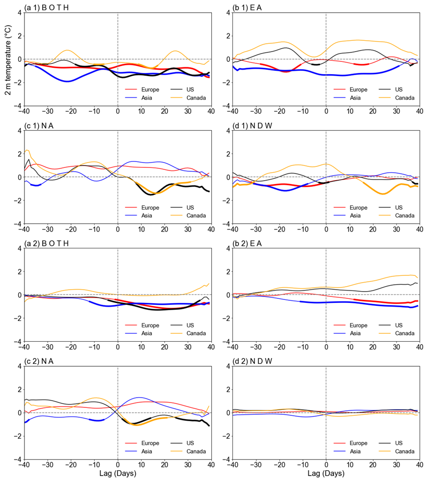
Figure 4 Evolution of the area-averaged t2m anomalies (units: K) from day −40 to day 40 over four regions (I–IV), including Europe (40–70° N, 0–60° E), Asia (40–70° N, 60–140° E), United States (30–46° N, 70–120° W), and Canada (46–60° N, 60–120° W) for (a) BOTH; (b) EA; (c) NA and (d) NDW events from two datasets: (a1–d1) ERA5 and (a2–d2) historical simulations by CESM2-WACCM. The thickened part of the line denotes the composite at the 95 % confidence level.

Comparing ERA5 and historical simulations by CESM2-WACCM, the composite t2m anomaly amplitude in model simulations is relatively weak and less significant in the pre-SSW period. Consistent with ERA5, cold anomalies persist from pre-SSW to post-SSW periods over both continents for the BOTH type in the model simulations. Further, the persistent cold anomalies over Asia from pre-SSW to post-SSW periods are also present in model evidence for the EA type. The reversal of t2m anomalies from positive to negative over North America and from negative to positive over Asia is also confirmed by model simulations for the NA type. Both ERA5 and CESM2-WACCM simulations show that the t2m anomalies over both continents are weak and insignificant most of the time during the NDWs (Fig. 4d1 and d2).

3.3 Analysis of isentropic potential vorticity

In order to further explore the process of cold air activity, an analysis of the isentropic potential vorticity (IPV) is investigated for the three types of DWs and the NDW. According to Eq. (1), the IPV is proportional to the absolute vorticity and static stability. In the case of equal vorticity, the cold air mass usually has a higher potential vorticity value due to its relatively larger static stability, which can be used to track the cold air activity on the isentropic surface (Hoskins et al., 1985; Lu and Ding, 2015). The 315 K isentropic level has been used to track the cold air sources by detecting the movement of high IPV center (Jeong et al., 2006). The composite evolutions of IPV anomalies are shown in Fig. 5 for all types of events based on ERA5 and CESM2-WACCM simulations. For the type BOTH, a patch of high IPVs appear from North Pacific 30–20 d prior to the event and gradually move southeastwards in the following period, which finally reach the North America for both datasets (Fig. 5a). During day 10 to 20, anomalously high IPV air moves to 45° N and even more southward, with the anomaly amplitude gradually weakened. Significant negative IPV anomalies develop over Greenland, consistent with the local anomalous high (see Fig. 3e), which helps advect cold air to eastern North America. In contrast, there are two high IPV centers in Eurasia, one over Europe, and the other over Central Asia. The anomalously high IPV center over Europe has remained stationary and continues to intensify. The high IPV center over Central Asia is more stable from day −30 to −10 and redevelops from day 0 to 20.

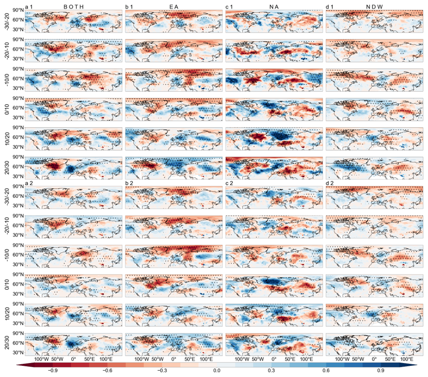
Figure 5 Composite isentropic potential vorticity (IPV) anomalies (shadings; units: PVU, 1 PVU $={\mathrm{10}}^{-\mathrm{6}}$ m² K kg⁻¹) at 315 K for (a) BOTH, (b) EA, (c) NA, and (d) NDW events from two datasets: (a1–d1) ERA5 and (a2–d2) historical simulations by CESM2-WACCM. The composite is based on the mean of 10 d intervals. The dots mark the composite anomalies at the 95 % confidence level using the t-test.

For the EA events, the high IPV center in the North Atlantic is weak and significant high IPV anomalies appear in Europe (Fig. 5b). The high IPV anomalies develop in North Atlantic soon after the SSW onset, and the Arctic is nearly covered by the positive IPV anomalies. Another positive IPV anomaly center is detected over North Asia since day −30 to −20, which diminishes from day −20 to −10 and redevelops from day −10 to 10. The high IPV patch moves southeastward to East Asia after day 10, indicating cold air outbreaks in local regions.

For the NA events, the high IPV center first appears over North Pacific from day −20 to −10, which is still active from day −10 to 10 (Fig. 5c). The positive IPV anomaly intensity weakens from day 0 to 10 and then redevelops in the later period. Further, it is also noticed that a large patch of positive IPV anomalies form over North Atlantic after the SSW onset, which is nearly motionless. Similar to BOTH events, the blocking pattern denoted as a wide range of negative IPV anomalies over Greenland is observed, and the upstream winds can advect cold air to eastern North America.

For the NDW events, the IPV anomalies are relatively weak, and the positive IPV anomalies are scattered and less organized over the land (Fig. 5d), consistent with the distribution of t2m anomalies. Weak positive IPV anomalies primarily appear over the oceans and are nearly motionless. It is also observed that a narrow band of positive IPV anomalies exists from the west to east across Canada during day 20 to day 30.

3.4 Total precipitation

Previous studies have shown that SSWs not only influence the cold air outbreaks, but also affect the rainfall anomalies (King et al., 2019; Oehrlein et al., 2021). Negative NAM phases are usually accompanied by a possible equatorward shift of the storm track, and a possible intensification of the moving cyclone at low latitudes (Afargan-Gerstman and Domeisen, 2020; McAfee and Russell, 2008; Thompson and Wallace, 2001). The composite precipitation anomalies from day 0 to 40 are shown in Fig. 6 to compare the rainfall anomaly sensitivity to the SSW type. The most pronounced common features for the four conditions in both ERA5 and CESM2-WACCM simulations are the rainfall dipole structure over North Atlantic–Europe. Positive rainfall anomalies form over Atlantic midlatitudes and the Mediterranean Sea, while negative rainfall anomalies form over Atlantic high-latitudes. This rainfall dipole is strong for BOTH and EA (Fig. 6a and b), while the intensity is relatively weak for NA and NDW (Fig. 6c and d). The positive rainfall anomaly in midlatitudes for NA is broken into two chains, one over the ocean, and the other biased toward the Eurasian land (Fig. 6c). Although the NAM fails to descend to the near surface, the rainfall dipole is biased farther northward for NDW (Fig. 6d).

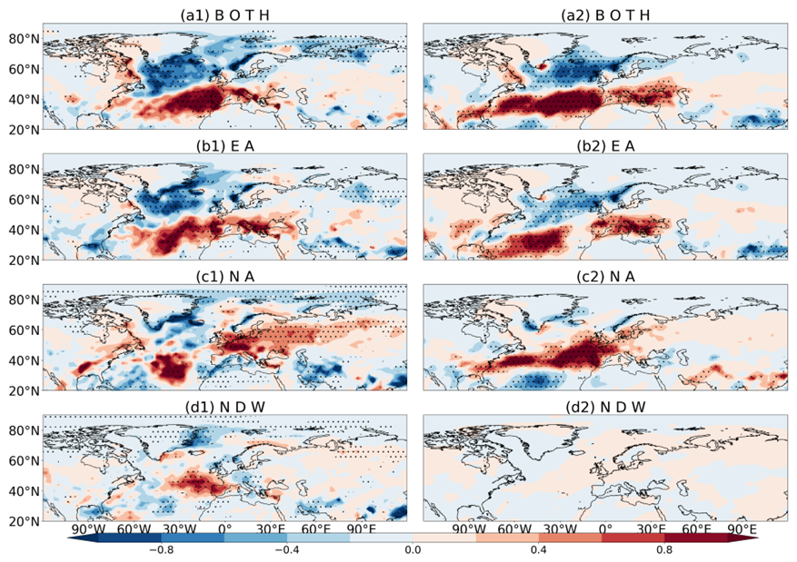
Figure 6 Composite precipitation anomalies (shadings; units: mm d⁻¹) for (a) BOTH, (b) EA, (c) NA and (d) NDW events after the SSW onset from two datasets: (a1–d1) ERA5 and (a2–d2) historical simulations by CESM2-WACCM. The composite is based on the mean of day 0 to 40. The dots mark the composite anomalies at the 99 % confidence level using the t-test.

Comparing ERA5 and CESM2-WACCM simulations, the rainfall dipole is consistently present for the BOTH and EA types (Fig. 6a and b). The negative rainfall anomaly lobe in high latitudes is much weaker for the NA type than for the BOTH and EA types for both datasets, although the positive rainfall anomaly band in midlatitudes is still present (Fig. 6c). In ERA5, the dipole rainfall anomalies are nearly absent due to the non-downward propagation of NDW SSWs, while the rainfall dipole disappears in model simulations for the NDW events (Fig. 6d).

4 Dynamic diagnostics

In order to compare the large-scale atmospheric dynamics between different types of SSW events, the composite circulation anomalies at 100 hPa and the sea level pressure anomalies are shown in Fig. 7. These results are intended to document the type-dependent dynamical characteristics of the circulation, rather than to establish a causal physical mechanism for the observed differences. In the pre-SSW period, the circulation structure is differently organized for three types of DWs and the NDW based on ERA5 and historical simulations by CESM2-WACCM. For the type BOTH, an anomalous high appears over Canada, and a low anomaly center forms over central northern Eurasia (Fig. 7a) with the polar vortex displaced toward North Asia. On the near surface, the negative NAM pattern has well developed, positive MSLP anomalies prevail over the Arctic, and negative anomalies develop over midlatitudes. The height anomaly distribution at 100 hPa for the type EA is similar to that for BOTH except that the height anomaly centers are further eastward situated (Fig. 7b). The anomalous high is situated at 60° E, while the anomalous low is situated over Northeastern Asia and Europe, implying that the polar vortex is likewise skewed towards Eurasia. Positive MSLP anomalies develop over the Arctic and northern Europe, while the negative MSLP anomalies form over northern Canada. For the type NA (Fig. 7c), the anomalous high at 100 hPa is centered over the Great Lakes, while the low covers most of northeast Asia. However, the near surface is covered by the anomalous low over most of the Arctic. These characteristics are markedly different from EA (Fig. 7f). For NDW, compared to DW, the polar vortex at 100 hPa is not significantly disturbed, and no significant low-pressure systems developed at sea level (Fig. 7d and e). Comparing the three types of DWs, the precursor circulation anomalies for BOTH are more baroclinic from the lower stratosphere to the troposphere (Fig. 7a and b), while for NA and EA, the circulation anomalies are nearly barotropic in high latitudes (Fig. 7b and c). The height anomalies at 100 hPa are much weaker for NDWs (Fig. 7d) than for DWs. The model results also suggest a weakening of the polar vortex at 100 hPa prior to DW events. At the surface, the spatial structure of the NAM, including the sign and location of the anomaly centers for different event types, broadly agree with those in the observational analysis. For the three types of DWs, during this period, negative anomaly centres emerged over Eurasia (or East Asia or Europe), indicating that the polar vortex was more inclined to shift towards Eurasia. This feature is consistent with the occurrence of cold anomalies across Eurasia during this period for all three types of DWs.

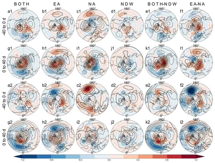
Figure 7 Composite 100 hPa geopotential height anomalies (contours; units: gpm) and sea level pressure anomalies (shadings; units: hPa) for (a, g) BOTH, (b, h) EA, (c, i) NA, (d, j) NDW, and the composite difference between (e, k) BOTH and NDW, (f, l) EA and NA before the SSW onset (top row) and afterward (bottom row) from two datasets: (a1–h1) ERA5 and (a2–h2) historical simulations by CESM2-WACCM. The composite is based on the mean of 40 d intervals. The dots mark the composite anomalies at the 95 % confidence level using the t-test.

In the post-SSW period, the Arctic is completely covered by high anomalies from the near surface to the lower stratosphere with a nearly barotropic circulation structure (Fig. 7g–j). In the lower stratosphere, the Arctic for all types of events is covered by the anomalous high, indicating the breakup of the stratospheric polar vortex. The positive anomaly amplitude for the three types of DWs in both ERA5 and model simulations is comparable, and their differences are mainly featured by midlatitude circulation anomalies. For BOTH, negative height anomalies are clearly present in midlatitudes with three centers, one over North Atlantic, one over Canada, and one over East Asia at 100 hPa (Fig. 7g). Similarly, the MSLP anomalies are well structured in a negative NAM pattern with the negative anomalies maximized over North Atlantic along midlatitudes. For EA, the negative height anomalies are not as detectable as for BOTH, and only the negative center over East Asia and North Atlantic is clearly observed at 100 hPa (Fig. 7h). On the near surface, the NAM structure is more clearly present in the Atlantic sector than in the Pacific sector. The local anomalous high over North Pacific disrupts the annular structure in the Eastern Hemisphere. For NA, the anticyclonic anomalies at 100 hPa are further biased toward the Arctic Canada, while nominal negative height anomaly band in midlatitudes for the negative NAM is only present over North Pacific (Fig. 7i). Similarly, the negative MSLP anomaly band is concentrated from the Western Europe to East Asia and North Pacific (Fig. 7i), different from the long anomalous low band in midlatitudes for BOTH and EA (Fig. 7l and i). For NDWs, although positive height anomalies are present over the Arctic in the stratosphere at 100 hPa (Fig. 7j and k), the amplitude is nearly half or one third of the strength for DWs. The MSLP anomalies in Arctic are very weak, while significantly negative MSPL anomalies over North Atlantic–Northern Eurasian are observed. Similarly, centres of negative anomalies are also observed at 100 hPa over the regions where cold anomalies develop in the three types of DWs. The circulation anomaly distribution in the post-SSW period is consistent between ERA5 and model simulations. The negative NAM structure is more clearly present in model simulations, possibly due to a much larger sample size in model simulations than in ERA5.

To further analyze the wave dynamics and to better understand the difference between the three types of DWs and the NDW, the E–P flux anomalies and the E–P flux divergence anomalies are shown in Fig. 8. The 10 d intervals before the SSW onset and afterward are examined for total planetary waves. For all types of SSWs, the upward propagation of planetary waves is enhanced before the event onset (Fig. 8a–d). Comparing the three types of DWs, the E–P flux anomalies are very comparable, and the anomalous E–P flux convergence center is structured differently (Fig. 8e and f). In both ERA5 and model simulations, the E–P flux convergence anomalies develop in the entire stratosphere for the type BOTH (Fig. 8a), while for EA and NA, the convergence anomalies are more concentrated around 50–150 hPa (Fig. 8b and c). The E–P flux convergence anomalies are weaker for the NDW than all types of DWs (Fig. 8f).

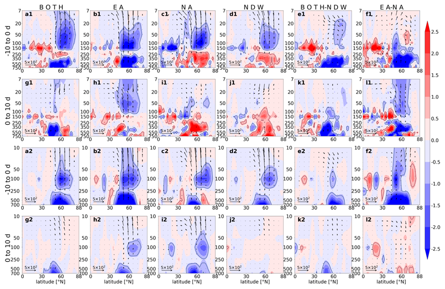
Figure 8 Composite E–P flux anomalies (vectors; units: F_y in 10⁴ kg s⁻², F_z in 10⁶ kg s⁻²) and E–P flux divergence anomalies (shadings; units: m s⁻¹) by planetary waves (sum of wave 1 and wave 2) for (a, g) BOTH, (b, h) EA, (c, i) NA, (d, j) NDW, and the composite difference between (e, k) BOTH and NDW, (f, l) EA and NA before the SSW onset (top row) and afterward (bottom row) from two datasets: (a1–h1) ERA5 and (a2–h2) historical simulations by CESM2-WACCM. The composite is based on the mean of 10 d intervals. The black line represents the 90 % confidence level for the composite E–P flux divergence anomalies.

After the SSW onset, the composite 10 d intervals E–P flux anomalies are also not identical for the three types of SSWs (Fig. 8g–i). The upward propagation begins to weaken for all types of DWs. However, the anomalous E–P flux convergence is still present in the lower stratosphere for type EA and NA. In contrast, weakening of the anomalous E–P flux convergence and the anomalous downward propagation of waves begins to form for the NDW (Fig. 8j). The relatively short lifetime and weak intensity of the wave forcing for the NDW likely explains the relatively weak intensity of the stratospheric disturbance. It is also revealed that the E–P flux divergence (or convergence) anomalies in the upper stratosphere are much weaker than in the lower stratosphere and upper troposphere for all events (Fig. 8g–j).

Figure 9 Same as in Fig. 8, but for planetary wave 1 E–P flux.

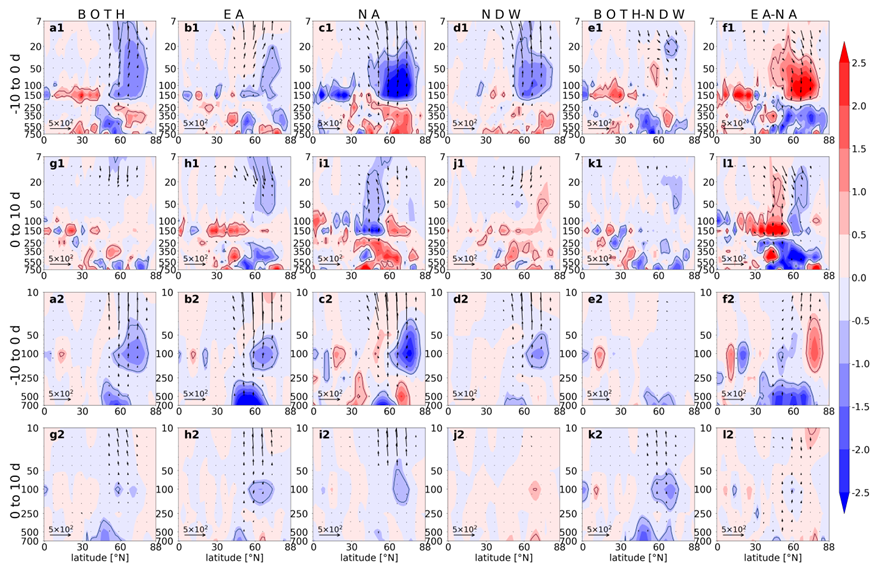
The contribution of the wave 1 and wave 2 to the total E–P flux and its divergence is shown in Figs. 9 and 10, respectively. A decomposition of the waves for E–P flux before the SSW onset can easily reveal the dynamical difference among the three types of DWs. Specifically, in the pre-SSW onset, the upward propagation of planetary wave 1 is strengthened for all events in both ERA5 and model simulations, and the E–P flux convergence anomalies by wave 1 also appear for all events (Fig. 9a–d). Moreover, it is obviously observed that the E–P flux convergence anomalies by wave 1 are strongest for NA out of all groups (Fig. 9f).

In the post-SSW 10 d interval period, the upward propagation of wave 1 is suppressed, and the contribution of wave 1 to the deceleration of westerlies (and therefore weakening of the polar vortex) nearly disappears (Fig. 9g–j). Namely, the E–P flux anomalies change the direction from upward to downward, and the E–P flux divergence anomalies are nearly zero. Wave forcing in midlatitudes is still present for DWs in ERA5, and the anomalous E–P flux convergence also persists in the lower stratosphere at midlatitudes (Fig. 9g–i). For model simulations, although the upward flux still lasts, the convergence of the E–P flux has rapidly declined.

Figure 10 Same as in Fig. 8, but for planetary wave 2 E–P flux.

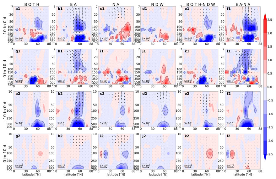
Similarly, the dynamics difference for the three types of DWs can be easily seen from the contribution of wave 2 to the total E–P flux and its convergence. In the pre-SSW periods, wave 2 cooperates with wave 1 to enhance the upward propagation of planetary waves and therefore the anomalous E–P flux convergence for BOTH and EA (Fig. 10a and b). Although the wave 2 is enhanced to propagate upward to the stratosphere for NA and NDW, no convergence of the E–P flux occurred, and the wave driven change for the circulation is not present (Fig. 10c1 and d1). For model simulations, BOTH and EA show strong E–P flux convergence anomalies. For NA and NDW, unlike in ERA5, weak E–P flux convergence anomalies also occur in the lower stratosphere.

This difference in the wave 2 forcing also exists in the post-SSW period for the three types of DWs (Fig. 10e–g). ERA5 shows that the vertical component of E–P flux anomalies by wave 2 reverses the sign for BOTH and NA (Fig. 10g and i), while the upward propagation of wave 2 is still present for EA (Fig. 10h1). As a consequence, the wave 2 forcing for the weakening of the polar vortex still persists after the SSW onset for EA, while this forcing for BOTH and NA types by wave 2 has terminated. Changes in the E–P flux anomalies and the divergence anomalies by wave 2 are not noticeable for NDWs (Fig. 10j). For model simulations, the E–P flux anomalies in various types of events have rapidly decayed, and the wave forcing has quickly disappeared.

The wave 1 and wave 2 can exert different effects on the stratospheric polar vortex (Baldwin et al., 2021; Lindgren and Sheshadri, 2020; Yang et al., 2023). The former propels the polar vortex displaced away from the Arctic, while the latter elongates and splits the vortex. Previous studies (Anstey et al., 2013; Kidston et al., 2015; Lehtonen and Karpechko, 2016) found that 2–3 weeks before the displacement SSW, it is anomalously warmer in the southeastern US and colder in Eurasia. These studies also found 2–3 weeks after the displacement SSW, the southeastern US is anomalously cold while Eurasia is unusually warm. In the month around the split SSW, the probability of both continents (North America and Eurasia) being cold at the same time is high. The different percentage of the displacement or split SSWs might further account for the different circulation and t2m anomalies for different types of DWs.

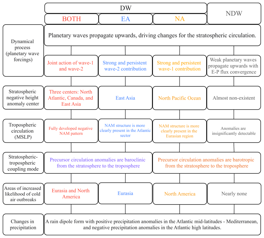
Figure 11 Schematic charts comparing the three types of DWs and the NDW. Aspects of comparison include preceding wave forcings by wave 1 and 2, the circulation pattern in the stratosphere, the stratosphere–troposphere coupling, ad the downward impact on near surface.

5 Conclusions

SSWs show strong inter-case variability for their impact on the troposphere and near surface. In this paper, SSWs are classified into different groups based on whether there is downward impact and on where the downward impact occurs. Using a newly proposed method, this study further classifies 52 SSWs in ERA5 and 273 SSWs in CESM2-WACCM into four groups: DWs with near surface impact over both Eurasia and North America (BOTH), DWs with impact over Eurasia (EA), DWs with impact over North America (NA), and NDWs. Finally, 33 DWs ($\mathrm{13}+\mathrm{14}+\mathrm{6}$) and 19 NDWs were identified from ERA5, while 119 DWs ($\mathrm{40}+\mathrm{51}+\mathrm{28}$) and 154 NDWs were selected from CESM2-WACCM simulations. Physical quantities in the CESM2-WACCM model tend to exhibit weaker amplitudes than those in ERA5, although it simulates the downward influence of the SSW effectively, successfully reproducing general features. The agreement between ERA5 and CESM2-WACCM does not imply that the underlying physical mechanisms are fully captured, but it does indicate that the identified type-dependent characteristics are reproducible across distinct data systems. To well distinguish the potential impact diversity of SSWs, the tropospheric circulation response and the near surface behaviors following these four types of events are revisited in this study. The main findings in this study are as follows and summarized in Fig. 11.

1. The mean intensity of NDW events in terms of the NAM and the circulation anomalies in the stratosphere and troposphere are nearly half weaker than DWs events, which is related to the definition of the events. Comparing the downward impact of three types of DWs, the persistency of the negative NAM pattern varies with the DW type. On average, the negative NAM signal in the lower stratosphere can last for >60 d for BOTH and EA, while it only lasts for ∼40 d for NA events. Further, the dripping pattern at the near surface exhibits a continuous negative NAM signal for BOTH and EA, while it is replaced by positive NAM at both the beginning and end of the SSW for NA.

2. A potential isentropic vorticity analysis reveals that anomalously high PV air can move southwards from the polar stratosphere and enter midlatitudes, thereby affecting the near ground. The cold anomalies over Eurasia and over North America have precursors in the upstream oceanic regions before the SSW onset. Anomalously low PV appears over North Atlantic 10–30 d before the EA onset and anomalous high PV forms over North Atlantic 0–30 d afterward. In contrast, anomalously high PV appears 10–20 d before the NA onset to 0–10 d afterward over North Pacific–Alaska. The PV anomaly evolutions for BOTH have a joint characteristic of both EA and NA. Namely, anomalously high PV forms over North Atlantic and North Pacific–Alaska as the anomalously low PV air enters the Arctic before the SSW onset for BOTH, while anomalously high PV air sweeps the continents soon afterward. In contrast, the t2m and 315 K PV anomalies are weaker and more scattered.

3. Adopting relative continental cold anomalies as the criterion for classifying SSWs, changes in precipitation anomalies are not so sensitive to the DW type as t2m anomalies. Following the onset of all types of SSWs, the rainfall band shows a southward shift especially over the Atlantic–Europe sector, exhibiting a rainfall anomaly dipole in the Western Hemisphere. Namely, the precipitation in subtropical Atlantic–Mediterranean Sea increases, while precipitation in high-latitude regions decreases. Previous studies have found that the southward shift of the precipitation band is associated with an equatorward shift in the storm track, and the intensification of moving cyclones at low latitudes (e.g., Thompson and Wallace, 2001; Huang and Xie, 2015).

4. The dynamical processes during DWs and the NDW are various before and after the SSW onset. In the pre-onset period, the negative NAM has been shaped at surface for BOTH and EA, while weak NAM still dominates at surface for NA, although anomalous high begins to form over the Arctic. In the pre-onset period, across all three types of DWs, the anomalously low centers are present over Eurasia, which signifies that following the collapse of the polar vortex, its remnant tends to move towards Eurasia. For BOTH, the anomalously low band stretching from the North Atlantic to North America represents the portion of the polar vortex that also extends towards the America. In the post-onset period, anomalously low centers exist above each cold anomaly region. This indicates that around the time of DWs, the polar vortex either shifts or splits, and the movement of the collapsed polar vortex is a significant factor in the region experiencing cold anomalies. The near surface NAM pattern is well organized with the midlatitude negative pressure anomalies over sea larger than over lands for BOTH and EA, while the pressure anomalies are larger over lands than over oceans for NA. For the NDW, the circulation anomaly amplitude is only half or even one third of that for DWs.

5. The dynamic differences for the three types of DWs are also featured by the wave activities. Firstly, the wave 1 forcing for them (BOTH, EA, and NA) shows a similar structure in the pre-onset period: the upward propagation of wave 1 increases, and the anomalous E–P flux convergence denotes a dissipation of wave 1 in the lower stratosphere. In the post-onset period, the enhancement of upward-travelling wave 1 terminates for BOTH and EA, but presents for NA. Secondly, the wave 2 forcing behaves in very different spatiotemporal structures: the wave 2 is enhanced to propagate upward in the pre-onset period for all types of DWs, but the wave dissipation in the stratosphere is only detected for BOTH and EA. In the post-onset period, the upward propagation of wave 2 is instantly suppressed for BOTH and NA, while the wave 2 forcing is still strong for EA.

6. Considering that displacement and split events have different impacts on the two continents (Anstey et al., 2013; Kidston et al., 2015; Lehtonen and Karpechko, 2016), a larger proportion of displacement SSW for NDWs and NA might explain their weak downward impact on near surface especially over Eurasia.

Compared with previous studies (Anstey et al., 2013; Domeisen et al., 2020), our study reveals the diversity of the DW events and distinguishes the potential impact on both continents in the Northern Hemisphere. The findings underscore the significant regional diversity in the tropospheric response to different SSW types, with distinct durations, intensities, and spatial patterns. These new classifications and syntheses of features can improve our understanding of weather and climate variability associated with SSWs, though the specific mechanisms responsible for their differing impacts await further investigation. This consideration is reasonable, because cold air outbreaks on both continents are not in pace most of the time (Butler et al., 2017; Yu et al., 2024). White et al. (2019) found that at least 35 events should be present to get robust differences between DW and NDW events. The sample sizes from CESM2-WACCM generally meet the case requirement in this study. Using more samples from CMIP6 multimodel outputs, a deeper understanding of different types of DW events is possible, left for future investigation.