Cloud condensation nuclei phenomenology: predictions based on aerosol chemical and optical properties

This study presents a comprehensive phenomenological analysis of cloud condensation nuclei (CCN) and aerosol properties – including activation properties, microphysical characteristics, chemical composition, and optical properties – across nine surface sites in different environments. Aerosol properties vary widely, reflecting the diverse environments, and controlling the CCN activation characteristics. Despite their critical role in aerosol–cloud interactions, CCN observations remain sparse and unevenly distributed, limiting global assessments of activation behavior. To address this gap, this study presents CCN predictive methods based on chemical composition combined with particle number size distribution (PNSD) data, and aerosol optical properties (AOPs). The chemical composition driven predictions are tested using three hygroscopicity schemes. All schemes overpredict the CCN concentrations (median relative bias; MRB = 13 %–15 %), although the two composition-derived CCN concentrations are markedly better predictors than the fixed-κ_chem assumption (MRB = 24 %). The AOPs-derived CCN prediction is based on two approaches: first, an extended empirical parameterization of Shen et al. (2019) (hereafter S2019) to 13 stations, which reduces bias from −27 % to −8 % and improves CCN agreement; and second, a random forest model that infers Twomey activation parameters (C and k) using both the S2019 variables and all the available AOPs. Including all AOPs reduces MRB from 19 % to 15 % and highlights the role of absorption in predicting CCN activation. These findings demonstrate that both chemical and optical measurements can provide a reasonable estimate of CCN concentrations when direct measurements are unavailable. These results will enable retrospective analyses of long-term aerosol time series to investigate aerosol–cloud interactions.

1 Introduction

Aerosol-cloud interactions (ACI) represent the largest source of uncertainty in quantifying the effective radiative forcing of anthropogenic aerosols, as highlighted in the IPCC: Intergovernmental Panel on Climate Change (2021) report. Within the total aerosol-induced effective radiative forcing of $-\mathrm{1.3}(\pm \mathrm{0.7})$ W m², ACI contributes approximately $-\mathrm{1.0}(\pm \mathrm{0.7})$ W m². This substantial uncertainty in ACI related processes arises primarily from an incomplete understanding of how changes in cloud droplet number concentration and size affect cloud water content and cloud spatial extent. These changes are driven mainly by variations in the abundance of cloud condensation nuclei (CCN) – aerosol particles that act as seeds for cloud droplet activation. Therefore, improving our understanding of CCN variability across spatial and temporal scales is essential to reduce uncertainties in global aerosol–cloud interactions and, by extension, climate projections (Seinfeld et al., 2016).

Reducing these uncertainties requires an improved understanding of aerosol properties across both long-term/large-scale and short-term/regional contexts. Key properties to reduce these uncertainties include aerosol number concentration, size distribution, chemical composition, and the ability of these particles to act as CCN. Over the past few decades, numerous studies have investigated the spatial and temporal variability of CCN and the factors controlling their concentrations in diverse (urban, continental, high-altitude, marine, and polar regions) environments (e.g., Ansmann et al., 2023; Deng et al., 2018; Gallo et al., 2023; Jurányi et al., 2011; Patel and Jiang, 2021; Rejano et al., 2021; Rose et al., 2010). However, most of these observations are based on short-term field campaigns and their comparability is limited due to differences in instrumentation and data processing, complicating efforts to quantify CCN impacts at the global scale. Thus, improving our understanding of aerosol-cloud interactions relies heavily on consistent and long-term measurements of particle number size distributions (PNSD), CCN number concentrations (N_CCN), aerosol chemical composition and hygroscopicity (Fanourgakis et al., 2019). A significant contribution to addressing this limitation was made by Schmale et al. (2017, 2018), who conducted a phenomenological study of collocated PNSD, chemical composition, and CCN measurements at 11 observatories – eight in Europe, two in Asia, and one in the USA. However, expanding this analysis to a global scale requires a more extensive dataset with measurements in regions not previously studied. To address this, Andrews et al. (2025a) recently compiled a dataset of PNSD, aerosol optical properties (AOPs), chemical composition and CCN at 10 observatories – three in the continental USA, two in South America, two in the Arctic and two in the middle of the Atlantic Ocean.

Even with the recent improvement in spatial coverage of CCN measurements and harmonized datasets (e.g., Andrews et al., 2025a and others), the limited current availability of direct measurements of N_CCN is still not adequate for climate research due to the high spatio-temporal heterogeneity of atmospheric aerosol. To overcome this limitation of regional/short-term measurements, several studies have investigated the use of more widely available aerosol parameters, particularly AOPs, for CCN estimation (e.g., Ghan et al., 2006; Shinozuka et al., 2009, 2015; Andreae, 2009; Jefferson, 2010; Liu and Li, 2014; Tao et al., 2018). These include properties such as the scattering coefficient (σ_sp), back-scattered fraction (BSF), and aerosol optical depth (AOD), which are routinely measured by ground-based networks (e.g., AERONET, GAW) and satellites. For example, Jefferson (2010) used σ_sp, BSF and single scattering albedo (SSA) to parameterize Twomey’s empirical CCN activation parametrization (Twomey, 1959), estimating the coefficients C and k. Previous studies have shown that C and k parameterizations are site-dependent and are affected by the loading and chemical composition of aerosol particles, respectively (e.g., Rejano et al., 2021). To address this site dependency, Shen et al. (2019) developed a CCN prediction equation based on in-situ aerosol optical properties and showed that correlations between the fit parameters could be used to reduce site dependency and improve generalization across regions.

The combination of aerosol chemical composition and PNSD within the framework of κ-Köhler theory has been widely applied to estimate CCN concentrations (e.g., Gunthe et al., 2009; Jurányi et al., 2010; Wang et al., 2010; Cai et al., 2022; Rejano et al., 2024). These estimates rely on different assumptions regarding the reconstruction of bulk aerosol hygroscopicity from individual chemical components (Schmale et al., 2018; Rejano et al., 2024). Reported closure agreement varies across studies, with aerosol mixing state identified as a key factor influencing CCN prediction accuracy (Cubison et al., 2008). The relationship between CCN spectral parameters and aerosol properties is often highly nonlinear because CCN activation depends not only on particle composition but also on size, with particles of different diameters activating at different supersaturation (SS) levels (e.g., Liang et al., 2022; Ervens et al., 2007; Nair and Yu, 2020). These nonlinearities limit the effectiveness of traditional linear analyses in fully capturing the complexity of aerosol CCN activity.

In recent years, machine learning (ML) has emerged as a powerful tool in atmospheric science, capable of capturing complex nonlinear relationships. To the best of our knowledge, the first application of ML to CCN prediction was introduced by Nair and Yu (2020) and later expanded by Nair et al. (2020), who developed a model using aerosol chemical composition and meteorological parameters under specific SS conditions. Rejano et al. (2024) applied a neural network at a high-altitude site with four inputs: N₈₀ (concentration of particles larger than 80 nm), the $\mathrm{OA}/{\mathrm{PM}}_{\mathrm{1}}$ ratio (organic aerosol to PM₁ mass concentration), the oxidation proxy f₄₄ (fraction of organic signal at m/z 44), and global solar irradiance. Liang et al. (2022) and Lenhardt et al. (2025) both applied random forest (RF) models, the former achieving robust CCN estimates from AOPs without chemical data and the latter identifying aerosol size as the main predictor of CCN–lidar backscatter relationships. More recently, Wang et al. (2025b) applied an ensemble of ML methods to six sites to determine the most important AOPs for CCN prediction. Collectively, these studies highlight the potential of ML to improve spatial and temporal characterization of CCN, with implications for satellite retrievals and climate models. However, applications remain largely site-specific, and generalizability across diverse environments is still uncertain, although Wang et al. (2025b) observed consistent patterns within similar site types.

In this study, observations from 9 observatories comprising collocated measurements of PNSDs, CCN number concentrations, CCN activation properties, and, in some cases, aerosol chemical composition and AOPs are analyzed. The stations cover a range of environmental conditions (continental, mountain, marine and polar). In what follows, first, the CCN phenomenology in terms of CCN concentration and activation parameters related to size distribution information is presented. Next, an overview of the chemical composition and in-situ AOPs, where available, is presented in connection with the observed CCN properties. CCN predictions based on aerosol chemical composition are evaluated and two additional approaches using aerosol optical properties, parameterizations and machine learning, are explored. Finally, the different prediction methods are systematically compared in the discussion section.

2 Methodology

This section first describes the location, environment type and the measurements available for each site. Then a brief description of the data quality control process is given. Next, we describe the CCN activation parameters and AOPs. Several CCN prediction schemes using the chemical composition and AOPs are presented. Finally, the random forest model methodology for CCN prediction is described.

2.1 Sites and measurement availability

This study considers 9 sites distributed across various environmental settings. All data presented here are described in Andrews et al. (2025a) and accessible at Andrews et al. (2025b). Although the Andrews et al. (2025a) dataset includes 10 sites, measurements at one of the sites (Ascension Island, ASI) were excluded from the present analysis due to unresolved instrument inconsistencies (e.g. temporal shifts in CCN-SMPS relationships) as reported by Che et al. (2025). Figure 1 shows the location, environment and measurement availability of each site, and Tables S4 and S5 in the Supplement present an overview of the characteristics of each station. Three observatories – MAO, COR and SGP – are located in continental environments, with MAO also occasionally influenced by urban emissions from the nearby municipality of Manacapuru (Brazil). One station – ENA – is situated in a marine region (north Atlantic Ocean). Additionally, ANX and MOS are located in the Arctic, where they sample both polar and marine aerosols. The MOS site corresponds to the MOSAiC (Multidisciplinary drifting Observatory for the Study of ArctIc Climate) expedition, where the instruments were deployed on an icebreaker frozen into and moving with the ice (Shupe et al., 2022). The remaining three observatories – GUC, SBS-CP and SBS-SPL – are situated in mountainous terrain in Colorado (USA), although these mountain sites are also subject to continental influences. The SBS-CP and SBS-SPL observations occurred during the STORMVEX (Storm Peak Laboratory Cloud Property Validation Experiment) field campaign (Mace et al., 2010), at the Steamboat Springs Ski Resort, separated by 5 km horizontally and 782 m vertically. The database includes both short-term campaigns with only a few months of measurements and long-term stations with several years of data, such as ENA and SGP. Further details on all sites and campaigns are provided in Andrews et al. (2025a).

From the available dataset developed by Andrews et al. (2025a), the data considered in this study include hourly-averaged measurements of N_CCN, aerosol activation properties, PNSD, total particle number concentration, chemical composition and AOPs (i.e., aerosol light-scattering and backscattering coefficients and absorption coefficient). All data considered have been previously processed, harmonized and quality assured and are freely available (Andrews et al., 2025b). All data are reported at standard pressure and temperature conditions (T_std=0 °C and P_std=1013 hPa) and at low relative humidity (<40 %) to ensure better comparability of results among collocated instruments at each site and across all 9 stations. The complete processing is described in detail in the data descriptor paper by Andrews et al. (2025a). A brief description of the instruments is provided below.

CCN concentrations were obtained with a CCN counter (CCNC), either the single-column (DMT1C) or the dual-column (DMT2C) version. Both models of CCNC had a column scanning across different SS with time, referred to as column A, and the DMT2C had an additional column measuring at a fixed SS, referred to as column B. Hourly-averaged PNSD data were derived from measurements made with a scanning mobility particle sizer (SMPS). The PNSD files also include the total particle number concentration measured by an independent condensation particle counter (CPC) over the same period. An integrating nephelometer and a particle soot absorption photometer (PSAP) provided aerosol optical data at most sites. The nephelometer measured aerosol scattering and backscattering coefficients at three wavelengths (450, 550 and 700 nm) and the PSAP measured absorption coefficients at 564, 529, and 648 nm. Optical measurements were made downstream of a switched impactor system so that both PM₁₀ and PM₁ values of the optical properties are available. Our analysis primarily relies on hourly PM₁₀ optical data, while PM₁ absorption data is used to complement the sub-micrometer composition data. The chemical composition data sets used in this study consist of hourly measurements from the quadrupole aerosol chemical speciation monitor (Q-ACSM, hereafter referred to as ACSM) and include the sub-micrometer mass concentration of particulate organics, sulfate, ammonium, nitrate, and chloride. Included with the ACSM data is the black carbon mass concentration derived from the PM₁ PSAP absorption coefficient at 529 nm.

Tables S4 and S5 provide an overview of the instrument models, available measurements, and site-dependent settings. Note that two (SBS-CP and SBS-SPL) and five (ANX, MAO, MOS, SBS-CP, and SBS-SPL) of the 9 sites do not have optical and chemical composition measurements, respectively (Fig. 1).

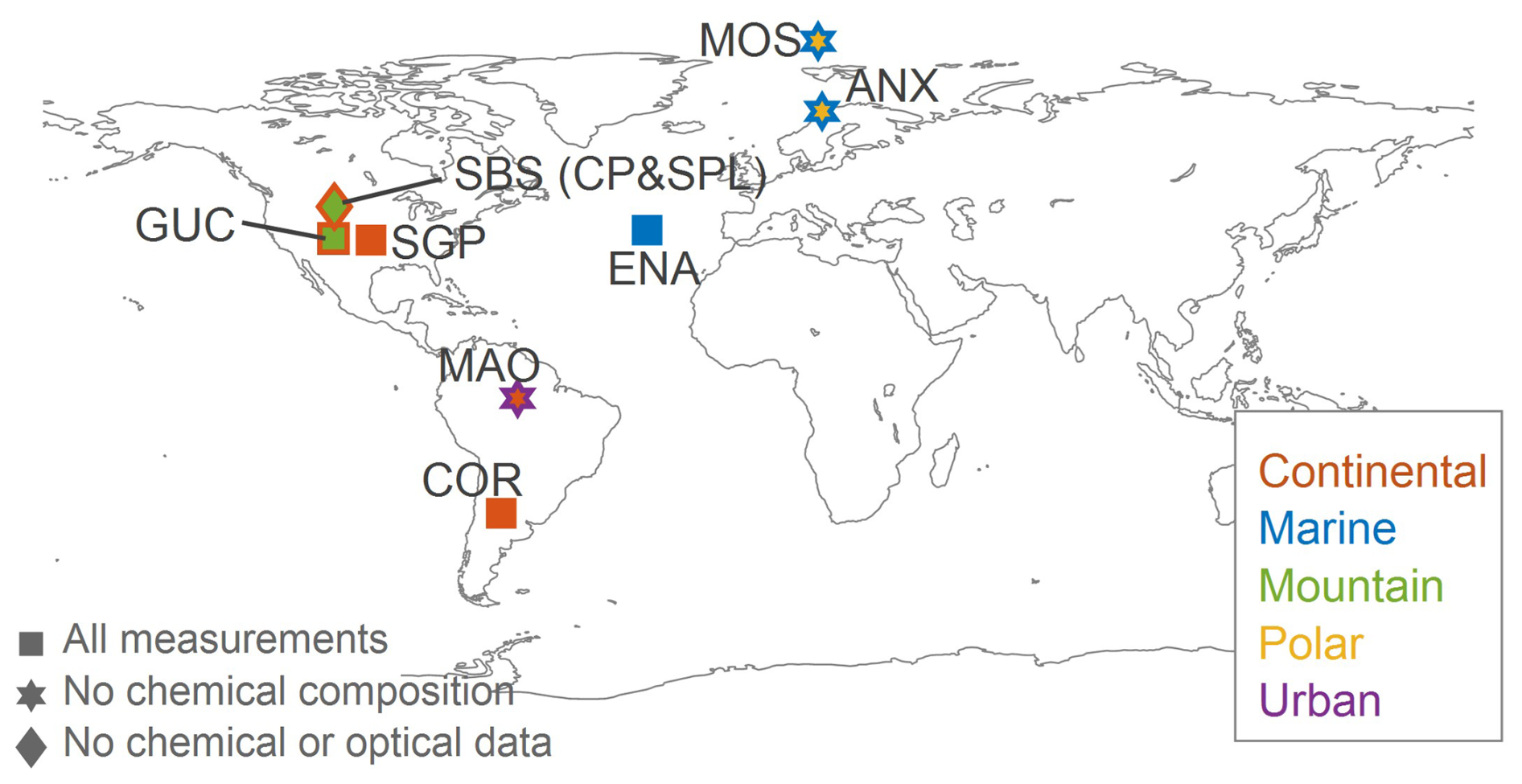
Figure 1 Map of sites considered in this study. Site type is indicated with different colors; if the outline is different than the fill color the site could be described by more than one type (e.g., polar and marine). MOS is a mobile deployment so the location represents the midpoint of shiptrack. Symbols indicate measurements availability.

2.2 Data quality control

To ensure confidence in the measurements, the datasets used in this study rely on multiple instrument intercomparison quality checks (closure studies) previously described in Andrews et al. (2025a). These checks identify potential inconsistencies between collocated instruments and ensure correct instrument functioning. In this study, we make use of two of these quality checks.

The first quality check applies to DMT2C instruments. CCN concentrations at 0.4 % supersaturation measured by column B are compared with those at the same SS from column A to ensure internal consistency. Data are excluded if the concentration difference exceeds 50 % (quality flag Qc_column_AB in the harmonized files). As shown in Fig. S4 of Andrews et al. (2025a), data from all sites with 2-column CCNC generally show excellent agreement.

The second quality check compares the total particle number concentration (N_tot) derived from the SMPS PNSD with that measured by a stand-alone CPC. In this study, SMPS–CPC concentrations are excluded if the relative difference exceeds 50 % (quality check Qc_CPC_SMPS described in Andrews et al., 2025a), but only when the contribution of particles smaller than 30 nm (N_<30) to N_tot is less than 20 % (condition applied in this study). This additional condition avoids removing data due to discrepancies related to the CPC's lower size cutoff and counting efficiency, especially during new particle formation events, when CPC counts can substantially exceed those inferred from the SMPS. Overall, the SMPS–CPC comparison across sites shows good agreement, as illustrated in Fig. S1 of Andrews et al. (2025a).

After applying these two quality checks, less than 2 % of the CCN column A data and a similarly small fraction of SMPS data were excluded across all sites. Figure S5 shows the instrument operating periods at each site after these quality checks are applied. Gaps may also exist due to periods when instruments were offline or not functioning properly, and for optical data, when sample RH inside the nephelometer exceeded 40 %.

For MOS, additional post-processing prior to applying the quality checks was required to remove periods affected by ship emissions (Boyer et al., 2023), using a pollution detection algorithm previously developed by Beck et al. (2022). The post-processing pollution detection algorithm was applied to the 5-minute resolution CPC data (MOS_smps_5min in Andrews et al., 2025b). As all instruments in this campaign measured from the same inlet, periods identified as polluted using the CPC are considered polluted for all instruments. The algorithm applies several filters: a power law filter (a=0.95, m=0.6), a threshold filter (10–10⁴ cm⁻³), a neighboring point filter, a median filter (30, 1.4), and a sparse data filter (30, 24). Only measurements classified as clean (66 % of the original data) are retained. After this filtering, minor additional removal of flagged SMPS (0.1 %) and CCN column A (0.07 %) data was applied. Figure S5 shows the available measurement periods at MOS after applying quality checks and the pollution detection algorithm.

2.3 CCN-derived properties

The Andrews et al. (2025a) data sets used in this study also include calculated parameters that can be used to characterize the CCN activation properties of the aerosol. These parameters are the activated fraction (AF), the critical diameter (D_crit), and the hygroscopicity parameter (κ_CCN). The activated fraction (AF) represents the fraction of particles that activate as CCN at a given SS, calculated as the ratio of CCN concentration to the total particle number concentration. In this study, AF values derived from CPC measurements were used at all sites except MAO, where SMPS data were used due to the lack of CPC measurements. The critical diameter (D_crit) represents the particle size above which all particles are activated into cloud droplets at a given SS. While the term critical diameter is sometimes used in Köhler theory to refer to the wet particle diameter at the maximum of the Köhler curve (corresponding to SS_crit), we follow the terminology adopted in the considered data set (Andrews et al., 2025b) and associated manuscript (Andrews et al., 2025a), as well as in Schmale et al. (2018), where D_crit denotes the dry diameter required for activation at a given SS. It can be derived by integrating the PNSD from the largest to the smallest diameters (Eq. 1) until the integrated number matches the measured CCN concentration at a given SS (Vogelmann et al., 2012; Jurányi et al., 2011). Alternatively, if D_crit is assumed and size distribution measurements are available but CCN data are not, CCN concentrations can be estimated as the number of particles larger than D_crit (Bougiatioti et al., 2009; Kulkarni et al., 2023; Rejano et al., 2024).

$$\begin{array}{}\text{(1)}& N_{\text{CCN}}\left(\text{SS}\right)=\underset{D_{\text{crit}}\left(\text{SS}\right)}{\overset{D_{\text{max}}}{\int }}{\displaystyle \frac{\mathrm{d}N}{\mathrm{d}\log D}}\mathrm{d}\log D\end{array}$$

The hygroscopicity parameter (κ_CCN) quantifies the ability of an aerosol population to absorb water from the environment and activate as cloud droplets (Petters and Kreidenweis, 2007). κ_CCN values derived from CCN measurements provide an estimate of the effective hygroscopicity of activated particles in the CCNC and exhibit a dependence on SS. Detailed derivations and equations for these parameters are provided in Andrews et al. (2025a).

2.4 ACSM-derived properties

Another approach to estimate the hygroscopicity parameter involves using chemical composition measurements. Since it is not feasible to determine the properties of each individual particle in the sample, an effective κ_chem for the entire population is estimated. Petters and Kreidenweis (2007) proposed a simple approximation (Eq. 2) to calculate κ_chem based on the hygroscopicity parameter (κ) and the corresponding volume fraction (ϵ) of each species (i) in the sample. This approximation follows the Zdanovskii-Stokes-Robinson (ZSR) approach, assuming a multi-component solution (i.e., a mixture of n different solutes) in equilibrium.

$$\begin{array}{}\text{(2)}& {\mathit{\kappa }}_{\text{chem}}=\sum _{i=\mathrm{1}}^n{\mathit{ϵ}}_i{\mathit{\kappa }}_i,{\mathit{ϵ}}_i={\displaystyle \frac{M_i/{\mathit{\rho }}_i}{{\sum }_{j=\mathrm{1}}^n{M}_j/{\mathit{\rho }}_j}}\end{array}$$

Here, M_i is the mass of species i and ρ_i its corresponding density. The index i refers to each individual species in the aerosol mixture. The summation in the denominator runs through all species (from 1 to n) each time. Further details on the κ_chem calculation under different assumptions, as well as its use in conjunction with measured size distributions used for CCN prediction, are explained in Sect. 2.6.1.

2.5 Optical parameters

The aerosol optical properties can provide insight into the size and chemical composition of aerosol particles. In-situ measurements of multi-wavelength aerosol scattering (σ_sp), back-scattering (σ_bsp), and absorption (σ_ap) coefficients are available at most sites (Tables S4 and S5). From these measurements, several optical parameters were calculated, including the back-scattered fraction (BSF), scattering Ångström exponent (SAE), absorption Ångström exponent (AAE), and single scattering albedo (SSA) following standard formulations (see Sherman et al., 2015; Shen et al., 2019).

The BSF indicates the relative abundance of smaller particles (D<0.3 µm) (Collaud Coen et al., 2007), while the SAE describes the wavelength dependence of σ_sp and serves as an additional proxy for particle size (Seinfeld and Pandis, 1998). BSF and SAE are sensitive to different segments of the aerosol size distribution (Collaud Coen et al., 2007); BSF is more responsive to particles in the lower part of the accumulation mode, whereas SAE is more influenced by particles in the upper part of the accumulation mode and the coarse mode. The AAE is calculated analogously to SAE and provides insight into aerosol composition, with values near 1 indicating the influence of dust or organic carbon (e.g., from biomass burning) (Bergstrom et al., 2007; Kirchstetter et al., 2004). The SSA quantifies the relative contribution of σ_sp and σ_ap and is also related to particle composition. All but one of the optical parameters were calculated at the native instrument wavelengths: BSF at 550 nm, SAE using 450 and 700 nm wavelengths, and AAE with 464 and 648 nm wavelengths. The exception is SSA where the absorption was adjusted to 550 nm to match the scattering wavelength.

2.6 CCN prediction methods

Although CCN concentration measurements are crucial for accurate representation of the CCN availability and variability across sites, these observations are not always available. As noted in the introduction, various methods have been developed to overcome this observational limitation and predict CCN concentrations (e.g. Gysel et al., 2007; Jefferson, 2010; Shen et al., 2019). In this section, we describe the three methods we apply to predict CCN concentration. A flowchart summarizing all CCN prediction methods is provided in the Supplement (Fig. S6).

2.6.1 CCN prediction using chemical composition

CCN concentrations can be predicted using κ-Köhler theory together with PNSD measurements (Eqs. 3 and 4 in Andrews et al., 2025a), once the bulk hygroscopicity parameter (κ_chem) has been derived. Below we describe the three schemes used to calculate κ_chem:

•  

  Scheme 1: Chemical composition measurements from the ACSM and the BC mass concentration are considered, so Eq. (2) can be expressed in terms of three main components: organics (OA), inorganics (IA), and black carbon (BC) (Eq. 3). This approximation has been shown to provide a reliable estimate of the effective aerosol hygroscopicity (e.g., Bougiatioti et al., 2009; Rejano et al., 2024).

  $$\begin{array}{}\text{(3)}& {\mathit{\kappa }}_{\text{chem}}={\mathit{\kappa }}_{\text{OA}}{\mathit{ϵ}}_{\text{OA}}+\sum _i\left({\mathit{\kappa }}_{{\text{IA}}_i}{\mathit{ϵ}}_{{\text{IA}}_i}\right)+{\mathit{\kappa }}_{\text{BC}}{\mathit{ϵ}}_{\text{BC}}\end{array}$$

  The contribution of inorganic aerosols to κ_chem includes several inorganic salts present in the atmosphere, such as ammonium nitrate, ammonium sulfate, ammonium bisulfate and sulfuric acid. The volume fractions of these salts are determined using the simplified ion pairing scheme from Gysel et al. (2007). The densities and κ values used for each component are summarized in Table S6 in the Supplement.

•  

  Scheme 2: To better understand the influence of black carbon on aerosol hygroscopicity, Scheme 2 excludes BC from the κ_chem calculation, focusing only on the hygroscopic components (inorganic salts, acids, and organics), which aligns with approaches commonly used in previous literature (e.g., Almeida et al., 2014; Schmale et al., 2018; Rejano et al., 2024). Comparison of both schemes allows for a clearer evaluation of the extent to which BC modulates the overall hygroscopic behavior of the aerosol population.

•  

  Scheme 3: To complement these two approaches, Scheme 3 is introduced, in which a constant value of κ_chem=0.3 is assumed. This scheme aims to serve as a simplified reference, independent of aerosol chemical composition. The value of 0.3 is commonly used in the literature as representative of average aerosol hygroscopicity under diverse atmospheric conditions (e.g., Schmale et al., 2018; Pringle et al., 2010). Pringle et al. (2010) report global mean κ_chem values of 0.27 for continental regions at the Earth's surface, supporting the use of 0.3 as a reasonable approximation for bulk aerosol hygroscopicity.

2.6.2 CCN prediction using optical properties

The prediction of CCN concentrations from aerosol optical properties has been explored in several studies (e.g., Ghan et al., 2006; Jefferson, 2010; Shinozuka et al., 2009, 2015; Liu and Li, 2014; Rejano et al., 2021). In addition to exploring the ability of AOPs to estimate CCN concentrations, the main application of this approach is to improve satellite retrievals (e.g., Shinozuka et al., 2015). In Shen et al. (2019) (hereafter referred to as S2019), a new empirical parameterization was developed by analyzing in situ measurements at six stations representing different environments. S2019 investigated the relationships between CCN concentrations at different SS and AOPs, and derived the following parameterization that explicitly depends on the SAE, BSF, BSF_min (1st percentile of BSF data) and σ_sp of PM₁₀ particles:

$$\begin{array}{}\text{(4)}& \begin{array}{rl}{N}_{\mathrm{CCN},\mathrm{S}\mathrm{2019}}\left(\text{SS}\right)& \approx \left[(\mathrm{286}\pm \mathrm{46})\mathrm{SAE}\right.\\ & \cdot \ln \left({\displaystyle \frac{\mathrm{SS}}{\mathrm{0.093}\pm \mathrm{0.006}}}\right)(\mathrm{BSF}-{\mathrm{BSF}}_{min})\\ & \left.+(\mathrm{5.2}\pm \mathrm{3.3})\right]\cdot {\mathit{\sigma }}_{\mathrm{sp}}.\end{array}\end{array}$$

This parameterization is designed to be applicable to any site, regardless of its environmental conditions, and for any SS < 1.1 % and provides a basis for estimating N_CCN directly from optical measurements (Shen et al., 2019).

In this study, we first test the generality of Eq. (4) and assess whether its performance holds across a wider range of aerosol types. Then we apply the S2019 methodology to our 7 sites plus the 6 sites utilized by S2019 to develop a new equation based on 13 sites to see if it improves the predictions of N_CCN. The derivation is detailed in the Supplement (Shen methodology section) and leads to the following equation:

$$\begin{array}{}\text{(5)}& \begin{array}{rl}{N}_{\mathrm{CCN},\mathrm{new}}\left(\text{SS}\right)& \approx \left[(\mathrm{320}\pm \mathrm{78})\mathrm{SAE}\right.\\ & \cdot \ln \left({\displaystyle \frac{\mathrm{SS}}{\mathrm{0.089}\pm \mathrm{0.011}}}\right)(\mathrm{BSF}-{\mathrm{BSF}}_{min})\\ & \left.+(\mathrm{8.7}\pm \mathrm{9.3})\right]\cdot {\mathit{\sigma }}_{\mathrm{sp}}.\end{array}\end{array}$$

For the seven sites with available AOPs included in this study, the BSF_min is estimated as 0.11±0.01. Accounting for the uncertainties in the regression coefficients, the propagated relative uncertainties in the predicted CCN concentrations are 81 %, 34 %, 27 %, 26 %, 25 % and 25 % at supersaturations 0.1 %, 0.2 %, 0.4 %, 0.6 %, 0.8 % and 1.0 %, respectively. Applying the original S2019 parameterization (Eq. 4) to the same dataset yields uncertainties from 16 % to 52 %. The wider error range in the new fit is driven primarily by the larger standard deviation of R_min, defined as the first percentile of $N_{\mathrm{CCN}}/{\mathit{\sigma }}_{\mathrm{sp}}$ (see Supplement for details), which is ±9.3 cm⁻³ Mm compared to ±3.3 cm⁻³ Mm in S2019. It is important to highlight several methodological differences between our approach and that of Shen et al. (2019). Although both studies include measurements from the MAO site, in our analysis this site is treated as independent from that in S2019 due to differences in time periods and data constraints: we used data from 2014–2015 and applied a relative humidity (RH) filter (RH < 40 %), while S2019 only used 2014 data without RH restrictions. Furthermore, instead of applying a threshold of σ_sp>10 Mm⁻¹ as in S2019, our study used a less restrictive filtering approach by excluding only data (σ_sp, BSF and SAE) when σ_sp values were below 0.5 Mm⁻¹ and above the 99.5th percentile, allowing a broader range of scattering conditions to be considered. Differences in the treatment of CCN data may also contribute to the variability between the resulting parameterizations.

2.6.3 CCN prediction based on AOPs using the Twomey equation and a random forest model

The Twomey equation (Twomey, 1959) describes the relationship between supersaturation (SS) and CCN concentration (N_CCN) via a power law with parameters C and k:

$$\begin{array}{}\text{(6)}& N_{\mathrm{CCN}}\left(\mathrm{SS}\right)=C\cdot {\mathrm{SS}}^k.\end{array}$$

This relationship is depicted graphically in Fig. S7 (solid lines) for some of the sites considered here. While Fig. S7 shows the overall fits to the data for each site, C and k can also be found for each individual SS scan at each site. Previous studies have found strong correlations between C, k and various aerosol properties (Jefferson, 2010; Rejano et al., 2021). Here, machine-learning is applied to predict these parameters from AOPs.

Random forest (RF) is a machine learning method that relates target variables (here, C and k) to predictors or “features” (Breiman, 2001; Cutler et al., 2012; Grange et al., 2018). Its main tuning parameters are (a) the number of trees, (b) the number of features considered at each decision node, and (c) the minimum number of observations required in a terminal or “leaf” node (also known as minimum leaf size), which controls the depth and complexity of each tree. The RF model might give better predictions with more trees and more explanatory variables considered, but that also increases the computational cost. Here, we use combinations of AOP variables (σ_sp, σ_ap, BSF, SAE, SSA, and AAE) as predictors to train the model. The RF algorithm is trained on one portion of the data and then the results of the training are applied to the non-training or test data to validate the prediction. In this work, two different validation strategies are considered. First, our primary validation uses a stratified $\mathrm{70}/\mathrm{30}$ split: for each site, 70 % of scans are randomly chosen for training and the remaining 30 % for testing. These per-site subsets are then pooled across all sites to form single training and test sets. Second, as an additional check, we perform leave-one-site-out (LOSO) cross-validation – iteratively holding out one site for testing and training on the others – to assess how including or excluding any given station affects model performance and to verify that the $\mathrm{70}/\mathrm{30}$ approach yields valid results across all locations. The predictors are not scaled or normalized before processing.

We implemented RF in MATLAB with TreeBagger function considering 500 trees, using the default minimum leaf size value (1) and sampling all predictors at each split. Performance was assessed via out-of-bag (OOB) error, and feature importance via OOB-permutation (Breiman, 2001). The model was run once to find the features relevant for C and then again, on the same data, to find the features relevant for k. Normalized importance scores reveal the variables that most consistently predict C and k. These predicted C and k values are then plugged into the Twomey power-law (Eq. 6) to estimate CCN concentrations at any given SS.

3 Results

In this section, we present the results showing the phenomenology of aerosol and CCN activation properties for all the stations considered in this study and the CCN prediction outcomes. We first provide a general overview of aerosol microphysical and CCN activation properties to demonstrate the range and variability of these characteristics at the 9 sites. Next, we summarize the aerosol chemical composition and use them to predict N_CCN for the sites where ACSM data are available using κ_chem. Similarly, we summarize the observed AOPs, where available, and use them to predict N_CCN, using the S2019 and RF methods. Finally, in Section 4, we evaluate the various CCN prediction methods we have applied and make recommendations for future studies.

3.1 Overview of aerosol and CCN activation properties at 9 sites

A summary of aerosol and CCN parameters at 0.4 % supersaturation for each site is presented in Fig. 2 as normalized frequency distributions. To facilitate a direct comparison with the results of Schmale et al. (2018), the distributions were computed using the same or comparable binning methods and normalized to the total number of data points at each station. However, we focus our analysis on 0.4 % SS – rather than 0.2 % SS used by Schmale et al. (2018) because the measurements at 0.4 % SS undergo an additional quality check (see Sect. 2.2), ensuring greater reliability of the data. While other supersaturations ranging from ≈0.1 to 1 % have been reported in the literature, we emphasize 0.4 % SS here to provide the most robust dataset for analysis.

The leftmost column (Fig. 2a) shows N_CCN (colored solid line) overlaid with total particle number concentration (N_tot, black dashed line). The center column (Fig. 2b) shows D_crit (colored solid line) overlaid with the geometric diameter (D_geo, black dashed line) of the PNSD. The rightmost column (Fig. 2c) depicts the CCN hygroscopicity parameter (κ_CCN). Table 1 provides the median values together with the 25th and 75th percentiles (P25–P75) for the five parameters shown in Fig. 2 and for the activated fraction. All variables are referred to 0.4 % SS.

Stations located in polar environments (MOS and ANX) tend to have the lowest N_tot and N_CCN (Fig. 2a), which is characteristic of the Arctic maritime environment (Barrie, 1986; Schmale et al., 2018). These sites are representative of pristine environments with minimal local sources of aerosols, dominated by natural processes and occasional long-range transport from distant regions. A similar trend was observed in other Arctic sites such as Barrow (Alaska) by Schmale et al. (2018). Slightly higher N_tot and N_CCN are observed at the ENA marine site compared to the Arctic sites, consistent with this site being a remote marine location where aerosols are primarily influenced by natural sources such as sea salt and biogenic emissions (Quinn et al., 2023; Wilson et al., 2015). At ENA, enhanced particle concentrations are likely associated with local sources due to the proximity of the station to an airport (Gallo et al., 2020). Nevertheless, CCN concentrations at ENA remain relatively low, leading to an activated fraction of 0.26.

The three mountain sites (GUC, SBS-CP, SBS-SPL) exhibit higher N_tot and N_CCN at 0.4 % SS than the polar and marine sites. SBS-SPL shows the lowest N_tot and N_CCN of the three mountain sites. SBS-CP is a site where the difference between N_tot and N_CCN is particularly pronounced, with N_tot up to six times larger than N_CCN. Both distributions are relatively narrow, suggesting that limited aerosol sources influence the site. The region where SBS-CP is located experiences springtime dust transport from both local and remote sources, which affects overall hygroscopicity (Hallar et al., 2015). Although the SBS-SPL site is very close to the SBS-CP site (SBS-SPL is 5 km east of SBS-CP), the altitude difference (∼2500 m for SBS-CP and ∼3200 m for SBS-SPL) makes SBS-CP more susceptible to influence from the atmospheric boundary layer, while SBS-SPL is more likely to measure free troposphere aerosol in the cooler months when these measurements were made. SBS-SPL is frequently in-cloud which may also lower aerosol loading via wet scavenging (Hallar et al., 2025). The N_CCN distribution at GUC is broader and shows higher concentrations than SBS-SPL despite their similar altitude. This is related to the influence of biomass burning intrusions during June and September 2022 (Gibson et al., 2025) affecting GUC. The three mountain sites show low median activated fractions at 0.4 % SS (0.11, 0.24, and 0.19 at SBS-CP, GUC, and SBS-SPL, respectively) compared to other high-mountain sites reported in the literature (Rejano et al., 2021; Jurányi et al., 2011; Duan et al., 2023). This difference can be partly attributed to a substantial fraction of measurements being collected during winter months, when weaker photochemical aerosol production (Baltensperger et al., 1997; Barbaro et al., 2024) and more persistent free-tropospheric influence (Collaud Coen et al., 2011; Jurányi et al., 2011) lead to smaller, less hygroscopic particles and lower AF. Site-specific processes, including intercontinental dust at SBS-CP and SBS-SPL (Hallar et al., 2011) and occasional biomass-burning events at GUC (Gibson et al., 2025) may also contribute to the observed low AF.

Frequency distributions of N_tot and N_CCN for the continental sites are shifted to higher particle and CCN concentrations. These sites represent regions with a mix of natural and anthropogenic influences, where long-range transport of pollution and local emissions contribute to the aerosol burden. The highest concentration of particles is observed at COR (median value of 3017 cm⁻³, with concentrations above 10 000 cm⁻³), which is frequently affected by biomass burning from the Amazon and anthropogenic emissions from Chile and Argentina (Fast et al., 2024). MAO exhibits a broad N_CCN and N_tot frequency distribution with an extended tail at the upper end of the distribution. The high N_CCN (and N_tot) values at MAO are associated with the station being affected by the regional transport of biomass burning pollutants (especially in the dry season, July–December) and to the Manaus (city located 70 km upwind) urban plume (Rizzo et al., 2013). COR and MAO show similar activated fraction of 0.29 and 0.25, respectively. Slightly higher AF is observed at SGP (0.38) associated with higher CCN concentrations.

The center column of Fig. 2 allows us to compare D_crit and the size distribution D_geo at different sites. D_geo serves as a proxy for the aerosol size distribution. Notable differences are observed in both the position and amplitude of the frequency distributions, suggesting variations in aerosol composition and activation processes across locations. Overall, D_crit is generally shifted to higher values compared to D_geo, indicating that a substantial fraction of particles do not reach the CCN activation threshold at 0.4 % SS. A similar trend between D_crit and D_geo was observed at most of the sites analyzed in Schmale et al. (2018). However, at MOS, D_crit is lower than D_geo, meaning that at 0.4 % SS, most particles activate as CCN. The marine station ENA exhibits broad frequency distributions centered on larger values, with overlapping D_crit and D_geo, suggesting that only a fraction of the particles activate at 0.4 % SS (AF median value of 0.26). This aligns with the wide range of hygroscopicity values observed at ENA, reflecting a mixture of marine aerosols and other sources, likely local emissions such as the nearby airport.

Of the two polar stations, ANX exhibits a lower median D_crit (55 nm), indicative of relatively hygroscopic aerosols, whereas MOS shows a higher median value (85 nm). The D_crit at MOS is broadly consistent with previous short-term, episodic observations (Dada et al., 2022), which report ≈80 nm at SS = 0.29 % and ≈50 nm at SS = 0.78 % under background conditions. At mountain stations, SBS-SPL stands out with the lowest D_crit (59 nm) and the highest value of κ_CCN (0.35), indicating a significant fraction of hygroscopic aerosols. This high hygroscopicity value could be attributed to the influence of anthropogenic SO₂ plumes from nearby coal-fired power plants, which have been shown to enhance particle growth from NPF to CCN-relevant sizes and thus facilitate CCN activation at SPL (Hirshorn et al., 2022).

In contrast, SBS-CP exhibits broader distributions and higher D_crit values, suggesting a more diverse aerosol mixture influences this site than SBS-SPL. The GUC mountain site exhibits frequency distributions similar to those of continental stations, characterized by D_crit distributions shifted toward intermediate-to-high values. The bimodal distribution of D_geo observed at GUC indicates the presence of two distinct aerosol sources influencing the site, such as background continental aerosols and episodic contributions from biomass burning or dust transport, consistent with previous studies (Gibson et al., 2025). Among continental stations, SGP has the lowest median D_crit (76 nm), indicating a higher fraction of CCN-active aerosols compared to COR (82 nm) and MAO (98 nm). This is consistent with the higher κ_CCN and activated fraction observed at SGP.

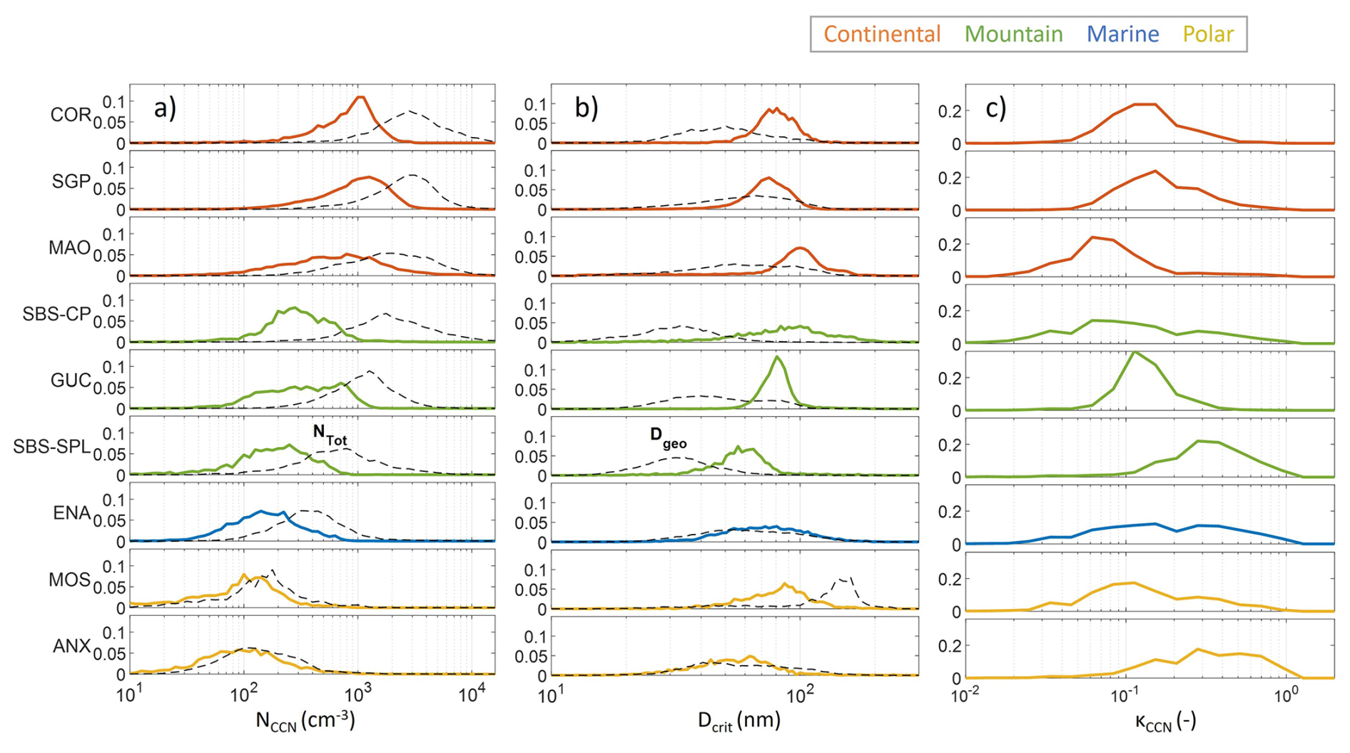
Figure 2 Normalized frequency distributions of (a) CCN number concentration (N_CCN) and total particle concentration (N_tot) in black, (b) critical diameter (D_crit) and geometric diameter (D_geo) in black and (c) hygroscopicity parameter (κ_CCN). All parameters related to CCN measurements are at 0.4 % SS.

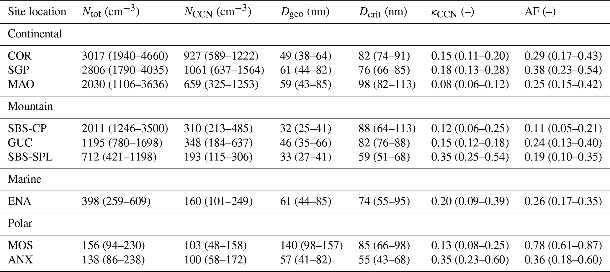
Table 1 Median values and percentiles 25th and 75th (P25–P75) of the total aerosol concentration (N_Tot), CCN concentration (N_CCN), geometric diameter (D_geo), critical diameter (D_crit), hygroscopicity parameter (κ_CCN) and activated fraction (AF) for each measurement location grouped by site type. All parameters related to CCN measurements are at 0.4 % SS.

3.2 Aerosol chemical composition and CCN prediction

3.2.1 Overview of aerosol composition

The aerosol sub-micrometer chemical composition measured with the ACSM is available at four of the nine stations (see Tables S4 and S5 for details). The operating temperature of the ACSM (600 °C) is not high enough to vaporize refractory components of the aerosol particles, thus only the non-refractory components can be analyzed. As a result, components such as elemental carbon, crustal material, and sea salt cannot be detected (Wu et al., 2016). To complement the ACSM chemistry, BC concentrations are derived from the PSAP absorption coefficient measurements. Figure 3 presents pie charts that illustrate the relative contribution of the species considered (organics, SO${}_{\mathrm{4}}^{\mathrm{2}-}$, NO${}_{\mathrm{3}}^{-}$, NH${}_{\mathrm{4}}^{+}$, Cl⁻, BC) to PM₁ at each site, along with the total mean mass concentration.

The mean concentration of PM₁ in the four sites ranges from 0.54 to 5.56 µg m⁻³, with varying contributions of the different components, reflecting the distinct aerosol characteristics of each location during the measurement period. Continental sites, COR and SGP, exhibit the highest concentrations (4.01 and 5.56 µg m⁻³, respectively). The mean value measured at SGP is slightly lower than that measured during 2010–2011 at the site (7 µg m⁻³) (Parworth et al., 2015) while for COR, the same value is reported in Fast et al. (2024) for the same campaign. In contrast, the lowest mass concentration is observed at the marine site ENA with a mean value of 0.54 µg m⁻³. The mountain site GUC exhibits an intermediate concentration of 1.57 µg m⁻³. These mean values are consistent with previous studies reporting PM₁ levels below 1 µg m⁻³ in remote and pristine marine environments over the Pacific, Atlantic, and polar oceans (Zhou et al., 2023), as well as with observations from high-altitude mountain sites where lower aerosol mass concentrations are typically found due to reduced anthropogenic influence (e.g., Fröhlich et al., 2015; Jimenez et al., 2009). It is important to note that the aerosol chemical composition exhibits strong seasonal variability, and the values presented here reflect specific measurement periods rather than long-term, annual averages, except at SGP, where long-term measurements are available.

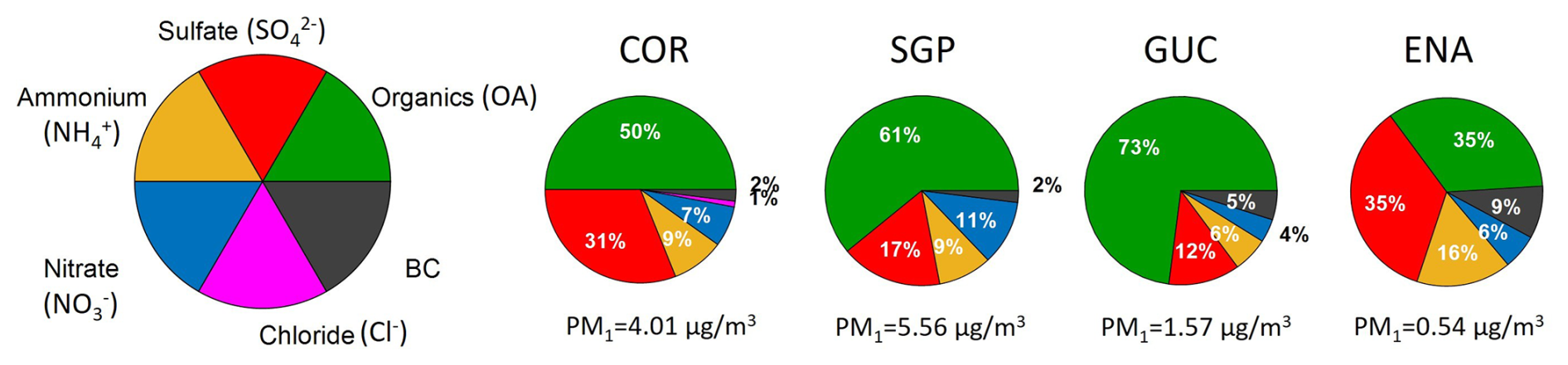
Figure 3 Pie chart of PM₁ mass concentration (OA, SO${}_{\mathrm{4}}^{\mathrm{2}-}$, NO${}_{\mathrm{3}}^{-}$, NH${}_{\mathrm{4}}^{+}$, Cl⁻ and BC) averaged for all the sites. Total mean PM₁ mass concentration for each site included.

For non-marine sites, the most abundant aerosol component is organic aerosol (OA), with the relative contribution ranging from 50 % at COR to 73 % at GUC. The OA concentration is highest at SGP (2.30 µg m⁻³), followed by COR (2 µg m⁻³). At the marine site ENA, sulfate and organic have the same concentration values (0.19 µg m⁻³), representing 35 % each of the total PM₁ mass. The presence of sulfate at this site is likely mainly associated with sea salt particles (Lin et al., 2022), consistent with its location in the marine environment. For COR, SGP, and GUC, sulfate is the primary inorganic component, with contributions of 31 % at COR, 17 % in SGP, and 12 % in GUC. The high contribution of SO${}_{\mathrm{4}}^{\mathrm{2}-}$ in COR has been linked to SO₂ emissions from small fires occurring outside Patagonia and the Atacama Desert (Fast et al., 2024).

The ammonium contribution ranges from 6 % at the GUC mountain site (0.10 µg m⁻³) to 16 % at the ENA marine site (0.009 µg m⁻³). At the continental sites, COR and SGP, ammonium accounts for 9% of the PM₁ mass concentration (0.36 and 0.50 µg m⁻³, respectively). Differences in ammonium contributions reflect both emission sources and total aerosol load. In continental environments, higher ammonium concentrations are driven by local and regional anthropogenic sources, including agriculture (especially livestock and fertilizer use), road traffic, industrial activities, landfills, coal combustion, and biomass burning (Anderson et al., 2003; Sutton et al., 2000). In contrast, the low total PM₁ mass observed at the marine site ENA results in a relatively high ammonium mass fraction despite low absolute concentrations. The ocean is one source for this ammonium (e.g., Quinn et al., 1988). Regional transport and secondary formation processes further enhance ammonium levels through the production of compounds such as ammonium sulfate and nitrate (Kang et al., 2018).

At most stations, nitrate plays a minor role (contribution less than 6 %) except for the continental stations (SGP; 11 % and COR; 7 %). SGP shows the higher mean NO${}_{\mathrm{3}}^{-}$ concentration (0.6 µg m⁻³), followed by COR (0.3 µg m⁻³). The higher contribution of nitrate at continental sites is associated with anthropogenic emission sources such as fossil fuel combustion, biofuel combustion, and agricultural fertilization (Jaegle et al., 2005).

Among BC concentrations, the highest contributions are observed at ENA (9 %; 0.05 µg m⁻³), likely influenced by local human activity near the station, which is located within half a kilometer of the local airport (Wilbourn et al., 2024). At the mountain site GUC, BC concentrations remain low (0.42 µg m⁻³), yet it accounts for 5 % of PM₁ mass. At continental sites, BC contributes less than 2 % with concentrations of 0.11 µg m⁻³ at SGP and 0.08 µg m⁻³ at COR.

3.2.2 Composition-derived hygroscopicity, κ_chem

The bulk chemical composition is used to estimate the overall κ_chem for each site, as explained in Sect. 2.4. In this study, κ_chem is derived based on three variations of Eq. (2): (i) including BC (Scheme 1); (ii) excluding BC (Scheme 2); and (iii) assuming a fixed κ_chem of 0.3 for all aerosols (Scheme 3). Figure 4a shows the resulting κ_chem values for each scheme at sites with available chemical composition measurements. Scheme 3, which assumes a constant value κ_chem regardless of site characteristics, is represented as a horizontal line at all stations. Among all sites and for both schemes 1 and 2, the marine station (ENA) has the highest κ_chem values (around 0.45), followed by the continental sites (COR and SGP, approximately 0.3), and the mountain site (GUC, around 0.23). In this context, applying a fixed value of κ_chem=0.3 (Scheme 3) tends to underestimate aerosol hygroscopicity in the marine environment and overestimate it at the mountain sites, while for the continental stations it provides a reasonably accurate approximation. The inclusion of BC in Scheme 1 results in slightly lower κ_chem values compared to Scheme 2 across all sites, since BC is assumed to be completely hydrophobic (κ_BC=0), thereby reducing the volume-weighted contribution of hygroscopic species. It is also worth noting that at marine sites, κ_chem may be underestimated due to the inability of the ACSM to detect refractory sea salt, which can significantly contribute to aerosol hygroscopicity in those regions (Deshmukh et al., 2025).

In general, κ_CCN is lower than κ_chem for all sites (see Fig. 4a and Table 1). Note that these two parameters cannot be directly compared since κ_CCN only accounts for activated particles in the CCNC and its calculation depends primarily on the dry aerosol size distribution and CCN concentrations as a function of SS, while κ_chem represents a bulk, mass-weighted hygroscopicity of all particles measured by the ACSM in the 40–1000 nm size range (Watson, 2017). As a result, if particles with diameters close to D_crit are less (more) hygroscopic than the larger particles dominating submicron mass, κ_CCN is expected to be smaller (larger) than κ_chem.

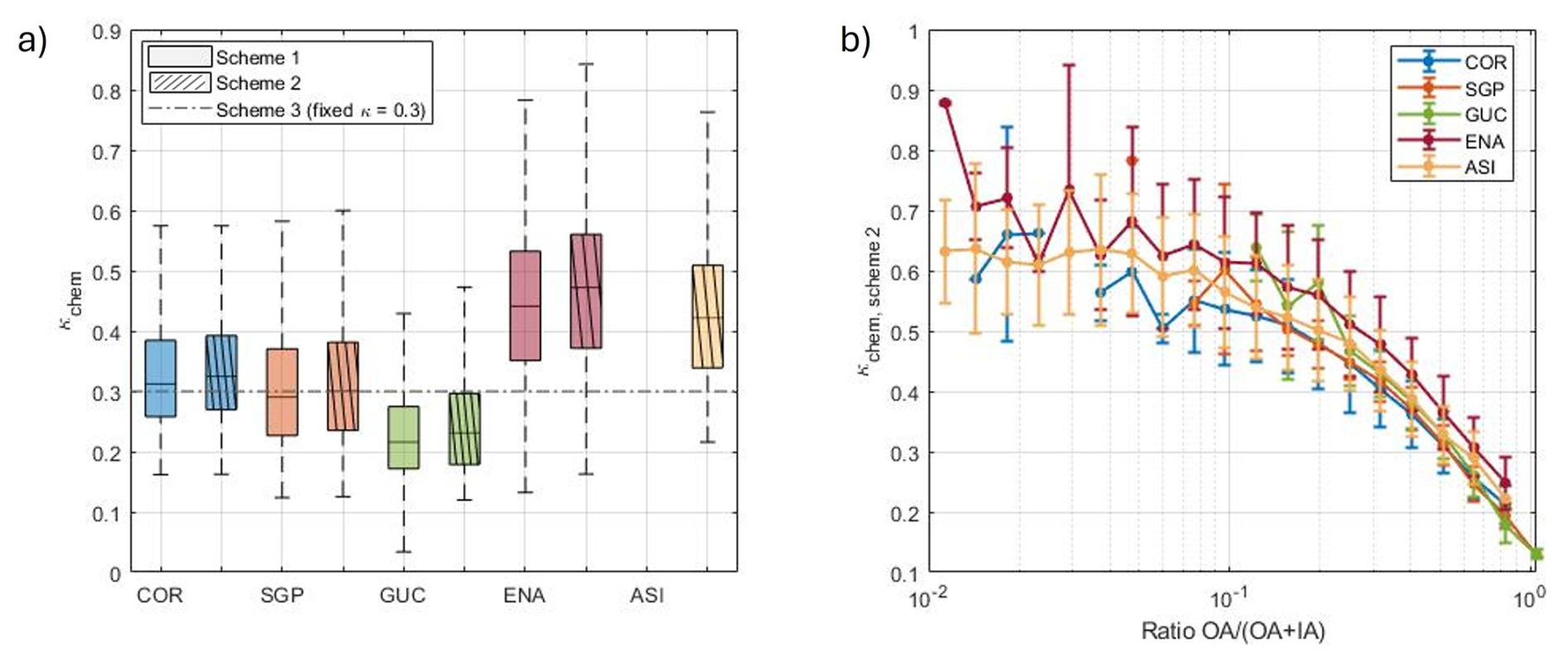
Figure 4 (a) Boxplots of κ_chem values for Schemes 1 and 2 at all sites with available chemical composition measurements. The line inside each box indicates the median, the bottom and top edges of the box represent the 25th and 75th percentiles, and the whiskers extend from the ends of the interquartile range (IQR) to the most extreme data points within 1.5 times the IQR. Scheme 3, which assumes a constant κ_chem=0.3, is represented as a horizontal line across all sites. (b) Relationship of the composition-derived κ_chem from Scheme 1 to the binned and averaged ratio of organic (OA) to total (OA + IA) aerosol components. The vertical bars denote the standard deviation.

Figure 4b shows the variation in the chemical composition derived hygroscopicity parameter (κ_chem) from Scheme 1 as a function of the binned and averaged ratio of organic to total aerosol mass concentration (OA $/$ [OA + IA]) for the four locations with ACSM measurements. The data were binned into 30 logarithmically spaced intervals between 0.01 and 10. The standard deviation is represented for each averaged value. Figure S8 in the Supplement provides the corresponding analysis using Scheme 2. For both schemes, a clear decreasing trend in κ_chem with increasing organic fraction is observed at all sites, reflecting that a higher contribution of organic aerosols reduces the overall hygroscopicity of the aerosol population. This behavior is consistent with the typically lower hygroscopicity of organic compounds relative to inorganic salts (Pöhlker et al., 2023). At low (OA $/$ [OA + IA]) ratios (<0.1) κ_chem becomes more noisy due to the lower number of data points, but appears to plateau between 0.5 and 0.7. When OA $/$ [OA + IA] < 0.1, the volume fractions ϵ_i of sulfate, ammonium, and nitrate dominate, as these are the main inorganic species at all sites (as shown in Fig. 3). Consequently, these species govern the sum in Eq. (2), and κ_chem plateaus at their volume-fraction-weighted average value (approximately 0.5–0.7; see Table S6).

This pattern is further supported by the results presented in Figs. 3 and 4a. GUC, the site with the highest organic fraction (73 %), exhibits the lowest κ_chem,Sch1 value among all the sites (∼0.2). Similarly, the other two continental sites, SGP and COR, have intermediate OA fractions (61 % and 50 %, respectively) and correspondingly low κ_chem,Sch1 values (∼0.25 and ∼0.30). In contrast, the marine site ENA, with a lower organic fraction of 35 %, presents a more balanced chemical composition – 35 % organics, 35 % sulfate, and 16 % ammonium – and a higher κ_chem,Sch1 (∼0.45). These results suggest that the organic fraction is a key driver of particle hygroscopicity, modulating the ability of the aerosol to take up water, thereby impacting the overall particle hygroscopicity (Aklilu et al., 2006; Dusek et al., 2010). In general, increasing organic fraction leads to a reduction in κ_chem, while a higher contribution of inorganic species – particularly sulfate and ammonium - increases overall hygroscopicity (Petters and Kreidenweis, 2007).

3.2.3 CCN prediction using κ_chem

Using the calculated κ_chem values, N_CCN is estimated using κ-Köhler theory (Sect. 2.6.1). The predictions are made considering the three κ_chem schemes. Figure 5 compares the predicted and measured CCN concentrations at all SS for the four sites where chemical composition measurements are available.

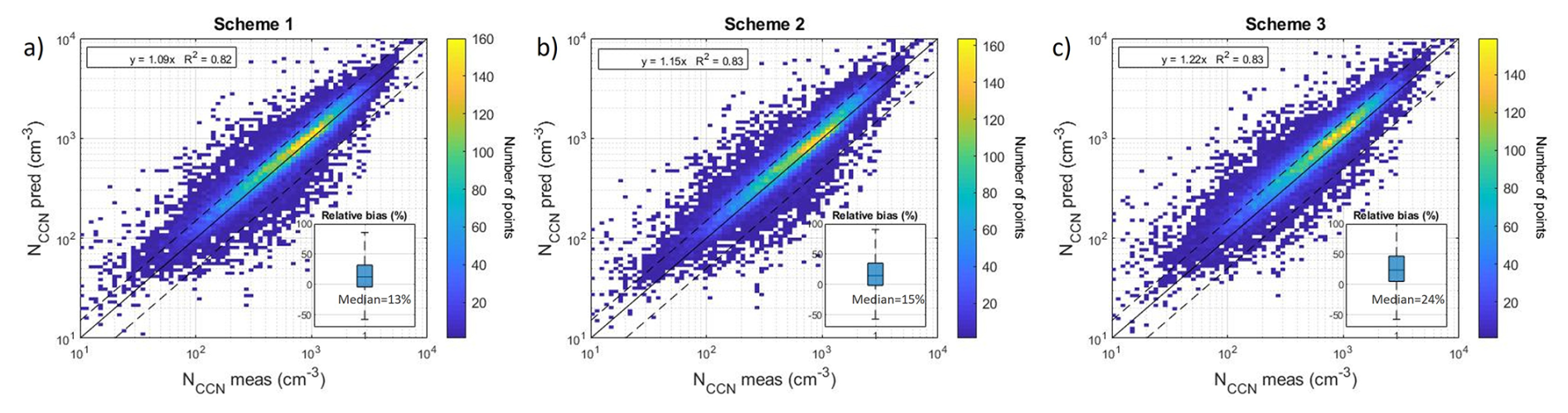
Figure 5 Log-log scatter plot of predicted CCN concentrations (N_CCN pred) with respect to the observed CCN concentrations (N_CCN meas) for all SS for all the sites using the three prediction schemes. Colored areas indicate the density of paired measurements, with color intensity representing the number of points within each log-spaced 2D bin (105×105 bins). A boxplot showing the relative bias is included- the central line represents the median, the box edges correspond to the 25th and 75th percentiles, and the whiskers extend from the ends of the interquartile range (IQR) to the most extreme data points within 1.5 times the IQR. Plots correspond to (a) Scheme 1 (κ_chem,Sch1), (b) Scheme 2 (κ_chem,Sch2) and (c) Scheme 3 (fixed κ_chem). The solid black line represents the 1:1 line and the dashed lines are the ±50 %.

Among the three schemes, the coefficient of determination (R²) is virtually identical (0.82 or 0.83), indicating a similarly strong correlation between predicted and observed CCN concentrations for all schemes. Scheme 1 (Fig. 5a) shows the best overall agreement with observations, with a slope of 1.09 and the lowest median relative bias (13 %), indicating a slight overall overprediction. Scheme 2 (Fig. 5b), which is best interpreted as a sensitivity test that indicates the impact of BC rather than as a different predictive approach, shows a slightly higher slope of 1.15 and a median relative bias of 15 %, reflecting a slightly higher overprediction compared to observations. However, the overall performance remains comparable to Scheme 1, with similar predictive capability despite not considering BC. Scheme 3 (Fig. 5c), which uses a fixed κ_chem, exhibits the highest slope (1.22) and the highest median relative bias (24 %), pointing to a consistent tendency to overpredict N_CCN. It must be considered that CCN concentrations predicted from κ_chem are based on the bulk, mass-weighted hygroscopicity of all particles measured by the ACSM as mentioned in Sect. 3.2.2. Because the CCNC measures the number of particles activated at the critical supersaturation (D_crit), and κ_CCN is inferred from number concentrations, the measured CCN concentration primarily reflects the hygroscopicity of particles near D_crit. Consequently, if particles around D_crit are less (or more) hygroscopic than the larger particles dominating the submicron mass, the predicted CCN concentration based on κ_chem may overestimate (or underestimate) the measured CCN concentration.

Figure S9 in the Supplement provides further insight into the performance of each scheme across different stations by showing the R² and median relative bias (MRB) values per site. Table S7 lists the number of data points available per site for each scheme. Continental stations (SGP, COR, GUC) exhibit a good predictive skill with a slight CCN concentration overestimation across schemes, while the marine site ENA shows larger sensitivity to hygroscopicity assumptions, largely due to the inability of the ACSM to detect sea-salt aerosol. Despite these limitations, the results are consistent with previous studies (e.g. Schmale et al., 2018), confirming that composition-derived κ_chem values improve CCN predictions, while a constant bulk κ_chem=0.3 provides a realistic first-order estimate of CCN number concentrations in diverse environments.

3.3 Aerosol optical properties and CCN prediction

3.3.1 Overview of aerosol optical properties

Aerosol optical measurements are available at 7 of the 9 sites (not available for SBS-CP and SBS-SPL). Figure 6 provides an overview of key aerosol optical parameters for all sites, including σ_sp and σ_ap, and four derived parameters: BSF, SAE, AAE and SSA. All measurements used in this analysis correspond to PM₁₀ aerosol size cut hourly data and are reported at 550 nm, or for the blue/red wavelength pair for SAE and AAE. As filtering criteria, for the calculation of the derived parameters, measurements with σ_sp<0.5 Mm⁻¹ were not considered and unphysical values were also excluded, i.e., SSA and BSF outside 0–1. In addition, negative SAE and AAE values were also excluded. On average, the combined constraints eliminated about 4 % of the data across all stations, although at MOS up to 17 % of the measurements were discarded. The filter responsible for most exclusions varied depending on the station, while the SSA constraint was generally the least restrictive, removing the fewest data points. It is important to note that the values presented here correspond to specific measurement periods rather than year-round averages, except for SGP and GUC, where more than 1 year of AOP observations are available and allow for a more representative characterization.

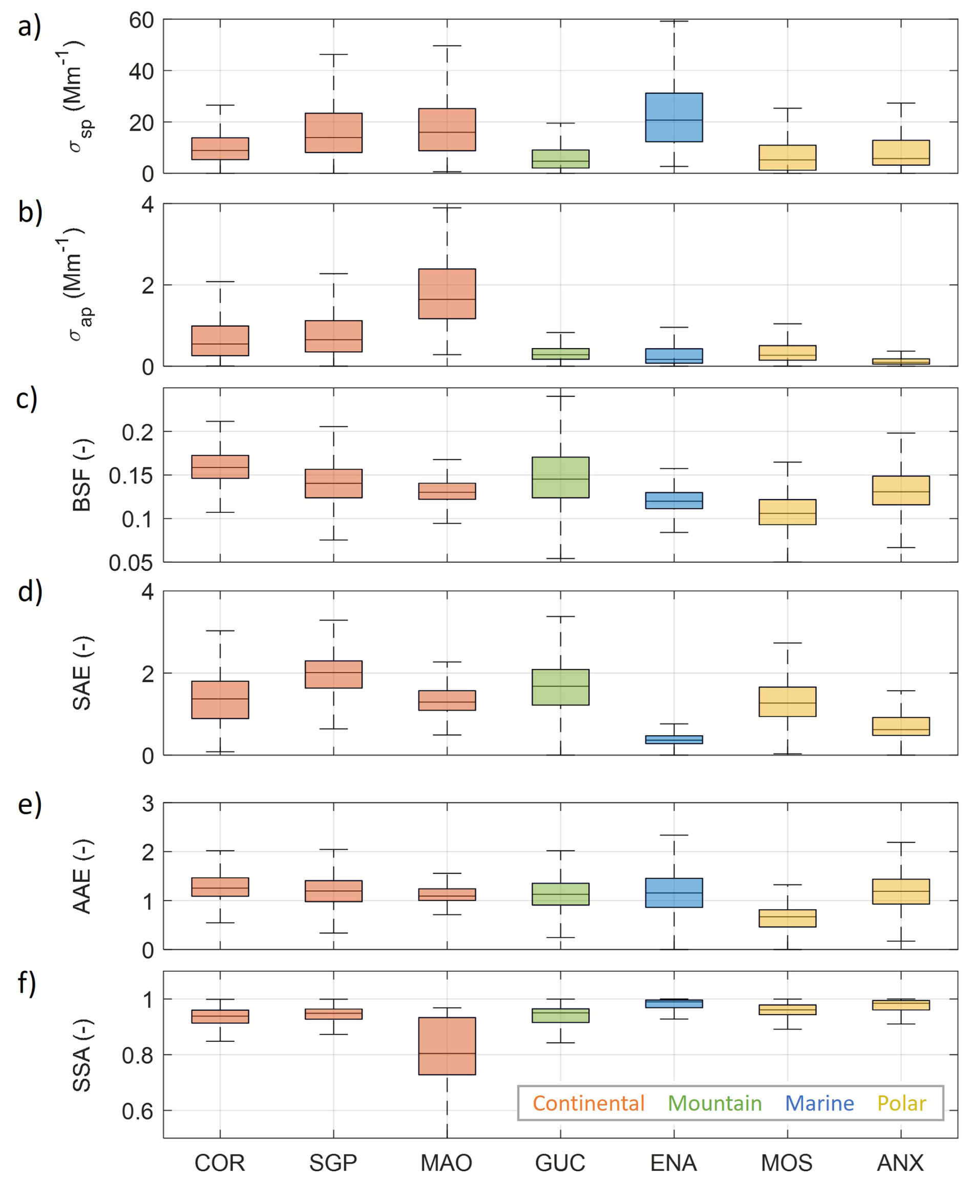
Figure 6 Boxplots of the distribution of aerosol optical properties at all sites. (a) σ_sp, (b) σ_abs, (c) BSF, (d) SAE, (e) AAE and (f) SSA. Median values (black lines), 25th–75th percentiles (black boxes) and the whiskers extend from the ends of the interquartile range (IQR) to the most extreme data points within 1.5 times the IQR.

The scattering coefficient (Fig. 6a) shows notable variability across sites, reflecting differences in aerosol loading. The highest median σ_sp is observed at the marine site ENA (e.g., 20.7 Mm⁻¹), which contrasts with the low PM₁ concentration at this site. This is likely due to high concentrations of supermicron sea salt particles commonly found in marine-influenced environments (Vaishya et al., 2011). This site is followed by MAO, SGP, and COR continental stations, with median values of 15.9, 13.9, and 8.9 Mm⁻¹, respectively. In contrast, the mountain site GUC and the polar locations (MOS and ANX) show the lowest median scattering coefficients (e.g., 4.7, 5.2, and 5.7 Mm⁻¹, respectively), consistent with their remote and cleaner atmospheric conditions. These findings align with those reported by Laj et al. (2020), where values below 10 Mm⁻¹ were observed for polar environments and mountain sites.

The absorption coefficient (Fig. 6b) has a different pattern at the sites than the scattering coefficient. The highest median σ_ap is observed at the continental site MAO (1.63 Mm⁻¹), suggesting a strong presence of absorbing particles, likely from biomass burning and anthropogenic emissions (Rizzo et al., 2013). This is followed by the other continental stations, COR and SGP, with median values of 0.55 and 0.65 Mm⁻¹, respectively. Marine and polar sites exhibit significantly lower values, with ENA, MOS and ANX showing median concentrations of 0.17, 0.27, and 0.09 Mm⁻¹. The mountain site GUC reports a moderate absorption level of 0.28 Mm⁻¹, in line with previous findings for high-altitude, remote locations, where aerosol absorption tends to be limited due to the absence of nearby combustion sources (Collaud Coen et al., 2018).

The back-scattered fraction (Fig. 6c), which is a proxy for particle size in the aerosol population, shows the highest median values at continental and mountain sites. The highest BSF is observed at COR (0.16), followed by SGP, GUC, and MAO, all with median values of 0.14. These elevated BSF values indicate a greater contribution from smaller particles. Marine and polar sites (ENA, ANX, and MOS) show smaller median BSF values in the range 0.10–0.13. This highlights the different source regimes - sea spray and remote transport in the marine boundary layer, and aged background aerosol in polar regions.

The scattering Ångström exponent (Fig. 6d) provides complementary information to BSF, as it is more sensitive to particles in the upper accumulation and coarse modes (Collaud Coen et al., 2007). The highest SAE values are observed at continental and mountain sites such as SGP (2.01), GUC (1.67), and COR (1.37), consistent with the prevalence of fine-mode aerosols from anthropogenic and biomass burning sources. At COR, frequent dust transport during the austral spring may explain its relatively lower SAE compared to other continental sites (Varble et al., 2019). In contrast, lower SAE values at marine and polar sites – ENA (0.36), ANX (0.62), and MOS (1.27) – suggest a stronger influence of coarse-mode particles such as sea spray or aged background aerosol.

The absorption Ångström exponent (Fig. 6e), which describes the wavelength dependence of aerosol light absorption and provides insight into aerosol composition, shows relatively consistent median values across most sites, ranging between 1.1 and 1.3, but with the higher percentiles ranging up to 2–2.5. The median values reflect locations with absorption primarily due to BC based on the Cappa et al. (2016) AAE $/$ SAE matrix, while the higher AAE values indicate occasional incursions of absorbing aerosols related to dust or biomass burning organics (Cazorla et al., 2013; Kirchstetter et al., 2004). In contrast, the polar site MOS exhibits a notably lower median AAE of 0.67. AAE values below 1 have been previously reported at remote Arctic and marine sites (Schmeisser et al., 2018), although such low AAE values may also be partially influenced by measurement artifacts in the presence of coarse-mode aerosols (Bond et al., 1999).

Finally, the single scattering albedo (Fig. 6f), which indicates the relative contribution of absorbing particles to aerosol extinction coefficient, shows high values across most sites (>0.9), suggesting the dominance of scattering aerosols. ANX, MOS, and ENA, which are all marine influenced, have median SSA > 0.95, while GUC, SGP and COR have median SSA values closer to 0.9. The lowest median SSA is found at MAO (0.80), indicating a relatively more absorbing aerosol mixture at this site consistent with anthropogenic and biomass sources.

3.3.2 CCN predictions using aerosol optical properties (S2019)

Following the S2019 methodology described in Sect. 2.6.2, Fig. 7 compares predicted CCN concentrations using (a) the original S2019 equation (N_CCN,S2019) and (b) the new version of the S2019 equation derived using the original data of S2019 and the data from the stations in this study (N_CCN,new), against measured CCN concentrations (N_CCN meas) for the seven sites with optical properties in this study and for all SS. The number of data points for each site used in the comparison – identical for both equations – is provided in Table S7 in the Supplement. The comparison shows an increase in the regression slope from 0.72 in plot (a) to 0.86 in plot (b), indicating a better agreement between predicted and measured N_CCN when using the new equation. The coefficient of determination (R²) remains unchanged (0.61), suggesting that the overall model performance is comparable in terms of explained variance. The median relative bias decreases in absolute value from −27 % in (a) to −8 % in (b) as the number of sites increases, indicating a reduced underestimation in the predictions. Meanwhile, the similar length of the MRB whiskers in both cases suggests that the variability remains comparable, even when a broader range of stations and aerosol conditions are included. However, the interquartile range decreases from 81 to 69, indicating reduced variability in errors. This reduction in MRB, together with the smaller IQR, reflects an improvement in prediction accuracy, with fewer extreme deviations and a more balanced distribution of errors. Consequently, the new equation provides CCN predictions that are more reliable and closely aligned with the measured CCN concentrations across the full range of conditions.

Figure S10 in the Supplement provides additional insight into the performance of both equations across different stations by displaying the site-specific R² and MRB (median relative bias) values. As observed in Fig. 7, the coefficients of determination remain largely unchanged between the two equations. For continental (COR, SGP, MAO) and mountain (GUC) sites, CCN concentrations tend to be slightly underpredicted with MRB < 0 (Fig. S10a), whereas overpredictions are more common at marine (ENA) and polar (MOS, ANX) sites (MRB > 0; Fig. S10a). The new equation (Fig. S10b) generally increases the predicted N_CCN values, leading to an overall improvement in prediction accuracy. Figure S11 shows the slope and relative bias for each measured SS between the predicted and the measured CCN concentrations considering the new equation. Excluding the lowest SS (0.1 %), both the slope and the median relative bias remain relatively stable across all SS values, indicating that the predictive equation performs consistently well regardless of SS. The larger deviation observed at 0.1 % SS may be attributed to the logarithmic function used to capture the dependence of N_CCN on SS. These results confirm that the original S2019 equation performs well across a wide range of conditions, even when evaluated with an extended dataset. However, the new equation proposed in this work provides a more accurate and balanced estimation of N_CCN, particularly by reducing systematic underestimation and improving agreement across the full concentration range.

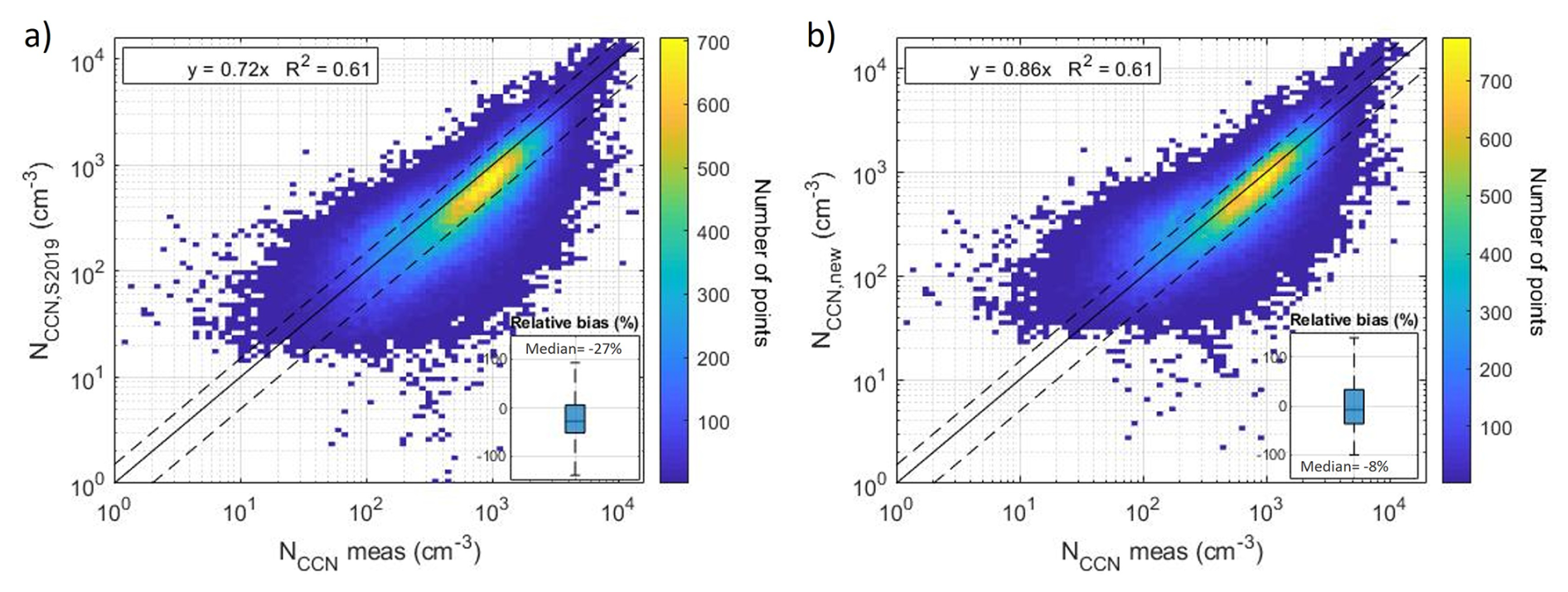
Figure 7 Log-log scatter plot of predicted with respect to the observed CCN concentrations (N_CCN meas) considering (a) equation in S2019 (N_CCN,S2019) and (b) new equation (N_CCN,new; based on 13 sites). The data plotted is only for the seven sites with optical data in this study (i.e., sites shown in Fig. 6). The solid black line represents the 1:1 line and the dashed lines are the ±50 %. Colored areas indicate the density of paired measurements, with color intensity representing the number of points within each log-spaced 2D bin (105×105 bins). A boxplot showing the relative bias is included. The boxes represent the interquartile range (25th–75th percentiles), with black lines indicating the median values and whiskers extending from the ends of the interquartile range (IQR) to the most extreme data points within 1.5 times the IQR.

3.3.3 CCN prediction with random forest model using optical properties

To further explore the potential of aerosol optical properties to predict CCN concentrations, a random forest model was implemented to estimate the C and k parameters of the Twomey equation. As input variables for the RF model, the same set of AOPs as in the S2019 equation (Sect. 3.3.2) is considered: σ_sp, BSF and SAE. All RF models considered in this work were trained with 500 regression trees, a number selected based on a convergence analysis of out-of-bag RMSE and R², which indicated stable model performance for both C and k parameters. Detailed model performance metrics for both training and test datasets including R², RMSE, MAE, and hyperparameter settings (number of trees, maximum depth) are provided in the Supplement (Random forest performance section). The close agreement between training and test metrics for both C and k indicates stable model behavior and no evidence of overfitting. Once the model is run, the predicted parameters are used to compute CCN concentrations across a range of SS. The performance of the model is evaluated by comparing these predictions based on RF with measured CCN values, allowing a direct comparison with the results of the S2019 parameterizations.

Figures 8 and S12 present the results of the RF model. Figure 8a and b display the relative importance of each input variable in predicting the C and k parameters, respectively, while Fig. S12 compares the observed and RF-predicted C and k parameters. For the C parameter, σ_sp contributes the most, followed by BSF and SAE, highlighting the dominant role of the total particle loading in determining the potential CCN concentration. In contrast, BSF is the most important variable in k prediction, followed by SAE and σ_sp, suggesting that the physicochemical properties of the particles, more strongly reflected by BSF and SAE, are more relevant to capture the chemical sensitivity embedded in k. These results are consistent with previous studies that have shown that C is primarily influenced by aerosol number concentration and total mass loading, while k reflects aerosol hygroscopicity and size distribution (Cohard et al., 1998; Jefferson, 2010; Vié et al., 2016; Rejano et al., 2021). Typically, high C values are found under polluted conditions with high particle number concentrations, whereas low k values are associated with particles exhibiting higher hygroscopicity and larger sizes (Martins et al., 2009; Pöhlker et al., 2016; Jayachandran et al., 2020). Thus, independent prediction of these two parameters offers valuable information on the abundance and physicochemical properties of aerosols that influence CCN activation.

Figure 8c shows the comparison of the predicted CCN concentrations, calculated using the RF-derived C and k values, and measured CCN concentrations across all supersaturations. The result shows a slope of 0.90 and a R² of 0.62, indicating good agreement between predictions and measurements. The inset boxplot shows the distribution of relative bias, with a median value of approximately 19 %, indicating an overall overestimation.

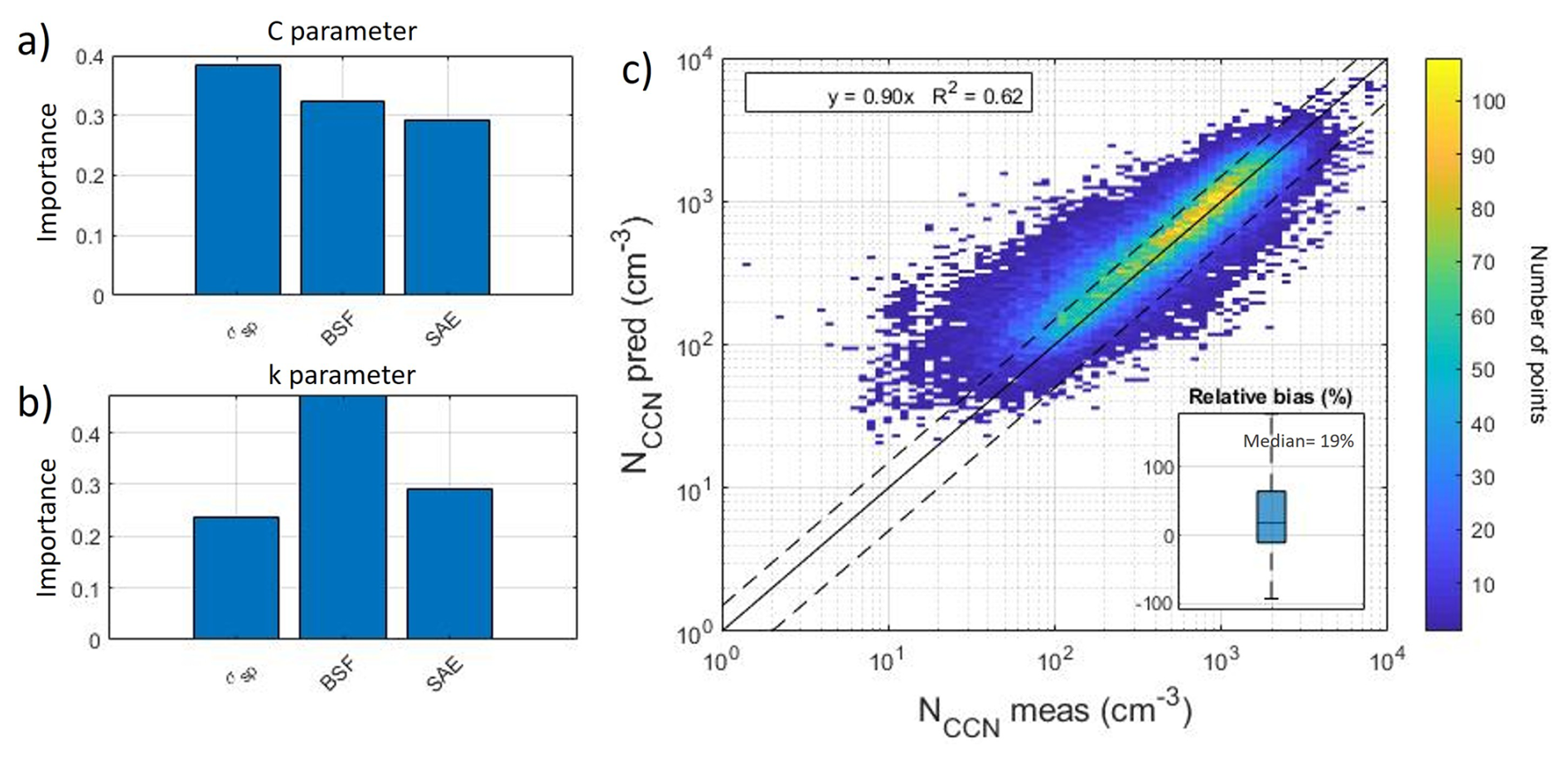
Figure 8 Importance of input variables in the random forest model considering AOPs used in S2019 (σ_sp, BSF, and SAE) for (a) C and (b) k parameters. (c) Log-log scatter plot of predicted (N_CCN pred) versus observed (N_CCN meas) CCN concentrations using a RF model to estimate the parameters of the Twomey equation. The solid black line represents the 1:1 line and the dashed lines are the ±50 %. Colored areas indicate the density of paired measurements, with color intensity representing the number of points within each log-spaced 2D bin (105×105 bins). A boxplot showing the relative bias is included. Boxes show the interquartile range (IQR, 25th–75th percentiles), with black lines indicating median values, and whiskers extending from the ends of the IQR to the most extreme data points within 1.5 times the IQR.

RF models can take advantage of additional informative features without a significant loss in predictive performance (Breiman, 2001) so, as the next step, the RF model is extended by including the full set of AOPs as predictors: σ_sp, BSF, SAE, σ_ap, AAE and SSA. Although some of these variables are strongly correlated (see Fig. S13), RF models are known to be robust to multicollinearity (Gregorutti et al., 2017). A full compilation of training and test metrics, as well as RF configuration details for this extended model is provided in the Supplement (Random Forest performance section). The improvement in R² and error metrics is consistently observed for both training and test datasets, indicating that the improved performance reflects increased predictive information rather than model overfitting. Figure 9c compares the predicted CCN concentrations – calculated using RF-derived C and k values from the full AOP set – with the observed values. The extended model achieves a slope of 0.91 and an R² of 0.69, slightly improving upon the performance of the RF model using only the three Shen-based variables (slope = 0.90, R²=0.62). The median relative bias also decreases slightly from 19 % (three-variable case) to 15 % (full AOP set), with comparable interquartile ranges (−92 to 180 vs. −88 to 145). To assess the RF models' performance across different SS levels, Fig. S14 presents the slope and median relative bias for both schemes. Results are consistent across the SS range, with slopes ranging from 0.80 to 0.99 and median relative biases between 8 % and 32 %, indicating that the predictive capability of the RF models is independent of SS. Finally, Fig. S15 in the Supplement shows site-specific R² values comparing predicted and measured CCN concentrations for both RF schemes, the S2019 AOPs (Fig. S15a) and the full AOP set (Fig. S15b). While the overall performance is similar, the inclusion of all AOPs – despite some strong inter-variable correlations (Fig. S13) – slightly improves both the coefficient of determination and the bias across all sites, supporting a more accurate prediction of CCN concentrations.

To better understand the source of these improvements in CCN prediction, we next analyze the relative importance of the input variables used to estimate the C and k parameters when using the full AOPs set. Figure 9a and b display the relative importance of each input variable in predicting the C and k parameters, respectively, while plots in Fig. S16 compare the observed and RF-predicted C and k parameters. AAE is identified as the most important input for the prediction of k (Fig. 9b), followed by SAE and BSF, suggesting that the chemical sensitivity embedded in k is better captured when accounting for absorption-related properties. For the prediction of the C parameter, BSF is the most important variable (Fig. 9a), followed by SAE and AAE, while σ_sp is of relatively lower importance. This result contrasts with the previous model (Fig. 8a), where σ_sp dominated, highlighting that including absorption-related parameters redistribute the contribution across variables. As previously mentioned, some of these variables are strongly correlated (Fig. S13) and the model tends to distribute the importance among correlated variables affecting overall predictive performance (Genuer et al., 2010).

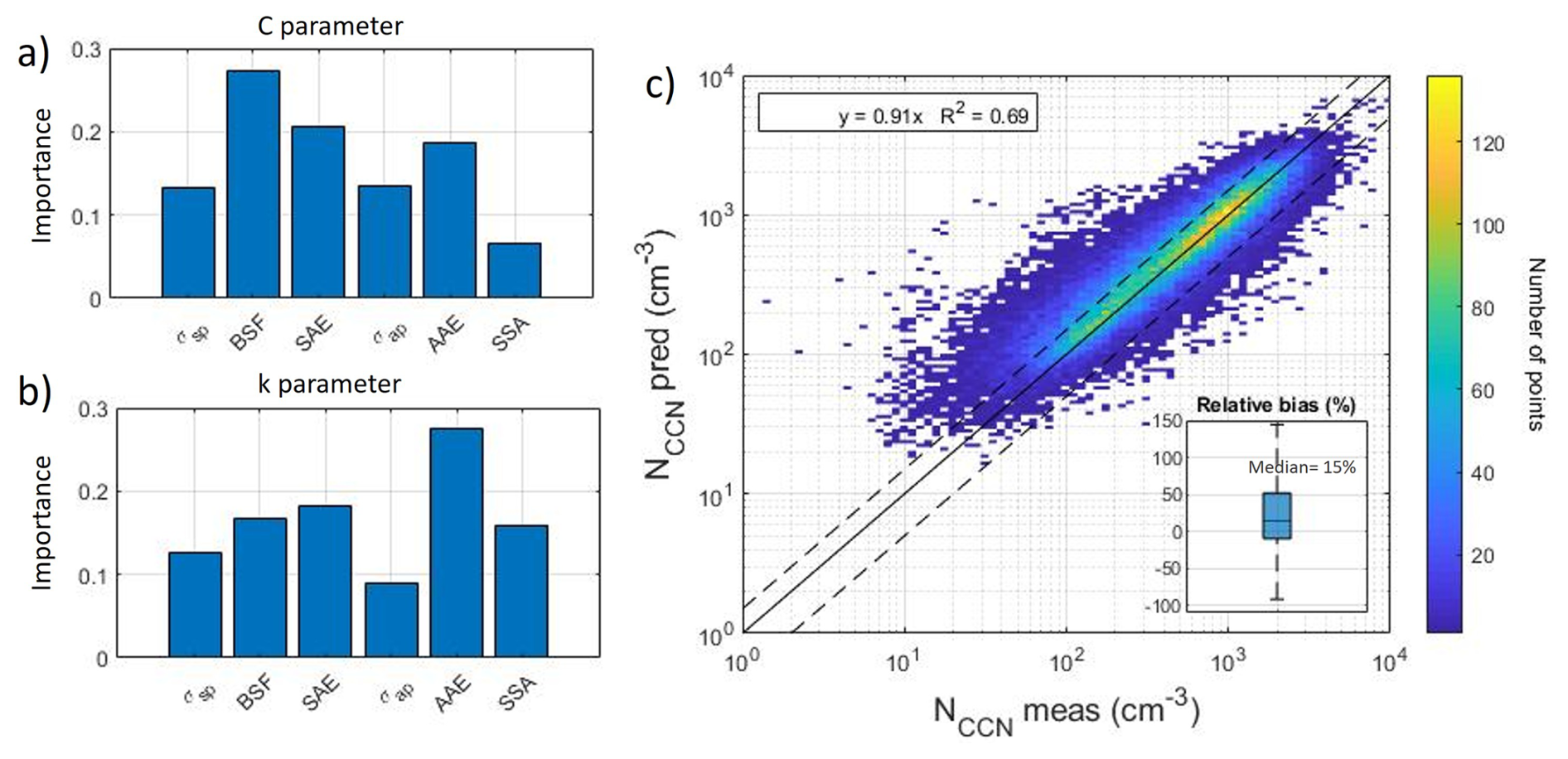
Figure 9 Importance of input variables in the random forest model considering all AOPs (σ_sp, BSF, and SAE, σ_ap, AAE, and SSA) for (a) C and (b) k parameters. (c) Log-log scatter plot of predicted (N_CCN pred) versus observed (N_CCN meas) CCN concentrations using a RF model to estimate the parameters of the Twomey equation. The solid black line represents the 1:1 line and the dashed lines are the ±50 %. Colored areas indicate the density of paired measurements, with color intensity representing the number of points within each log-spaced 2D bin (105×105 bins). A boxplot of the relative bias is included. Boxes show the interquartile range (IQR, 25th–75th percentiles), with black lines indicating median values, and whiskers extending from the ends of the IQR to the most extreme data points within 1.5 times the IQR.

To further analyze how different AOPs contribute to the prediction of the C and k parameters, Fig. 10 presents heatmaps of variable importance for models using different combinations of AOP inputs for C (Fig. 10a) and k (Fig. 10b). In these heatmaps, each row corresponds to a model run (the first row includes all AOPs; subsequent rows exclude one AOP at a time), and each column represents one of the six AOPs. Analyzing these heatmaps reveals that BSF remains the most important predictor of C, except when σ_sp, σ_ap, or BSF itself are excluded from the model. In these cases, the model shifts its reliance to a closely related variable: AAE becomes the dominant predictor when BSF is removed, while σ_ap and σ_sp substitute for each other when one is absent. This behavior likely reflects the partial redundancy and strong interdependence among BSF, AAE, σ_sp, and σ_ap. Indeed, their relationships are supported by the Spearman correlation coefficients (Fig. S13 in the Supplement): BSF and σ_sp are negatively correlated (${\mathit{\rho }}_{\mathrm{s}}=-\mathrm{0.41}$), σ_sp and σ_ap show a strong positive correlation (ρ_s=0.68), and BSF and AAE are moderately correlated (ρ_s=0.36). While these correlations help explain why certain variables gain importance when others are removed, it is important to note that RF variable importance also depends on how much each variable contributes to reducing prediction error across the ensemble, not solely on pairwise correlations (Breiman, 2001). For the prediction of k (Fig. 10b), the AAE is the most important predictor under the full model. Removing AAE shifts the top rank to BSF, again reflecting their correlation. This result highlights the RF model's ability to reallocate predictive importance among partially redundant features, relying on combinations of variables that together best capture the relevant information rather than depending on any single variable.

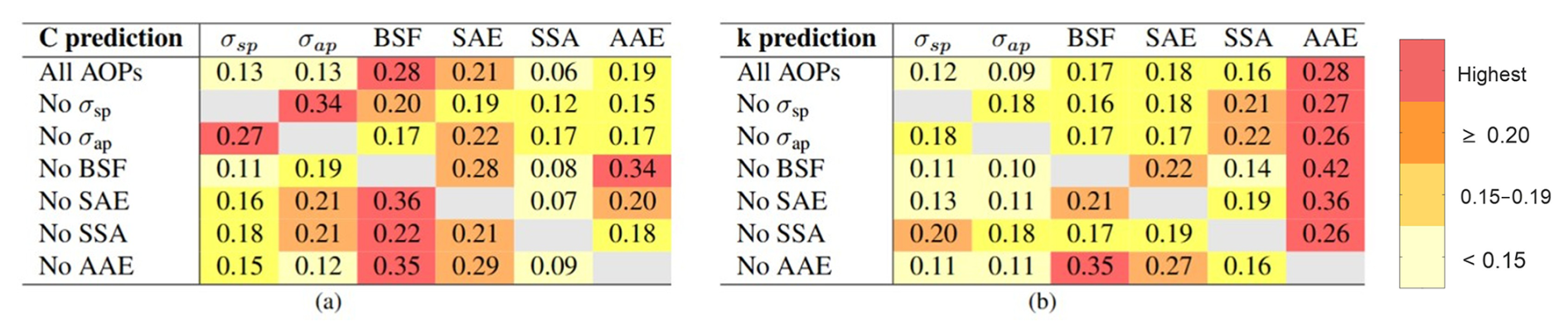
Figure 10 Heatmap of input variable importance in the Random Forest model for (a) C and (b) k parameters. Each row corresponds to a RF model in which one AOP has been removed, while each column represents the importance assigned to each available AOP in that model. The variable with the highest importance in each prediction is shown in red; importance values ≥0.20 are shown in orange; values between 0.15 and 0.19 in dark yellow; and values <0.15 in light yellow.

RF model results could be influenced by the differences in the availability of data at each measurement site, providing better results for those sites where datasets are longer. Therefore, to evaluate the influence of each location on model generalization when considering all AOPs, a LOSO cross-validation approach is applied as explained in Sect. 2.6.3. This analysis is intended to evaluate spatial robustness and site representativeness, rather than to provide an alternative global performance metric to the train-test and OOB evaluations discussed above. Figure S17 in the Supplement shows the variable importance for each site in the LOSO iteration. In each subplot, the name of the site excluded is indicated. The importance of predictors remains consistent across sites: AAE and SAE typically dominate the prediction of k, while BSF, SAE and AAE are more important for predicting C. This consistency confirms that no single site influences feature selection within the model. Notably, when SGP – the site with the largest number of observations – is excluded, some shifts in variable importance are observed. However, these changes are not large enough to affect the overall importance, suggesting that the $\mathrm{70}/\mathrm{30}$ approach used in the main analysis is not biased by the dominance of SGP data. Figure S18 in the Supplement shows the comparison between predicted and observed CCN concentrations at each excluded site. Slopes range from 0.38 in ENA to 1.87 in MOS, and R² values from 0.03 to 0.56. Although predictive performance remains good for most sites, the model shows reduced accuracy at marine and polar locations (e.g., ENA, MOS, ANX). This is likely due to the fact that the training data are dominated by continental stations, limiting the model’s ability to capture the distinct AOP characteristics of marine and polar environments.

A recently published study by Wang et al. (2025a) used an ensemble of multiple machine learning tools to investigate the ability of AOPs to predict CCN concentrations at 4 sites which are common to this study (SGP, GUC, ENA and MOS). As input variables, Wang et al. (2025a) uses σ_sp, BSF, SAE and SSA at the different wavelengths. The R² values obtained ranged between 0.2 to 0.63, depending on the predictive model construction. Their ensemble model was trained specifically for each site and for SS = 0.4 %, aiming at optimizing their predictive potential to the unique atmospheric conditions of each site. In our case, we decided to apply the RF model to the whole range of SS and to all sites together in order to provide a general model that performs reasonably well at most atmospheric conditions.

4 Discussion of CCN prediction methods

Direct measurements of CCN concentrations are less common than other aerosol properties, making reliable prediction from commonly measured variables an attractive and cost-effective alternative. In this study, we evaluated several CCN prediction approaches using co-located measurements at the selected sites. These include chemistry-based methods (three schemes differing in the treatment of BC and hygroscopicity assumptions), optical property-based approaches using empirical parameterizations derived from AOPs (the original Shen et al. (2019) formulation and a new parameterization developed here), and a machine-learning method, where a random forest model is used to predict the Twomey equation parameters C and k from aerosol optical properties.

In addition to these approaches, a widely-used particle number size distribution PNSD-based method is included here to enhance the discussion. In this approach, CCN concentrations are estimated by counting particles larger than the critical activation diameter (D_crit), assumed to be 151, 113, 82, 64, 53, and 50 nm for SS = 0.1 %, 0.2 %, 0.4 %, 0.6 %, 0.8 %, and 1.0 %, respectively. These values correspond to the median D_crit for each SS obtained from the median values across stations and fall within the range reported in previous studies (Bougiatioti et al., 2011; Jurányi et al., 2011; Schmale et al., 2018). The results of this PNSD-based approach are presented in Fig. S19 in the Supplement, showing the results across the 9 sites.

Figure 11a shows the MRB, which quantifies systematic deviations with positive values indicating overprediction and negative values underprediction, between predicted and measured CCN concentrations for all the methods. Figure 11b shows the median absolute error (MdAE) for each method, providing the typical magnitude of the prediction error in absolute units. It should be noted that these values are calculated across all SS and all sites where different methods can be applied. The simple D_crit approach exhibits the best overall performance, with a MRB of −2 % and the lowest MdAE (83 cm⁻³), indicating negligible systematic bias and high precision relative to the CCN concentrations typically observed at the studied sites.

The chemistry-based prediction approaches show slightly reduced performance compared to the D_crit method. Schemes 1 (including BC) and 2 (excluding BC) exhibit moderate overprediction (MRB < 15 %) and comparable MdAE values (98–100 cm⁻³), indicating reasonably good precision but a tendency toward positive bias. Scheme 3, which assumes a constant κ_chem=0.3, shows the largest bias (MRB = 24 %) and higher MdAE (141 cm⁻³), reflecting increased error dispersion. While less accurate, this approach still provides a useful first-order estimate when chemical composition measurements are unavailable, consistent with previous studies (Schmale et al., 2017; Rejano et al., 2024). The reliance on bulk chemical composition, which assumes particles are internally mixed and chemically homogeneous regardless of size (Wang et al., 2010; Ren et al., 2018), and assumptions about the chemical species present (e.g., sulfate forms, organic types) in the atmosphere, can increase uncertainty in chemistry-based CCN prediction methods (Schmale et al., 2017; Rejano et al., 2024).

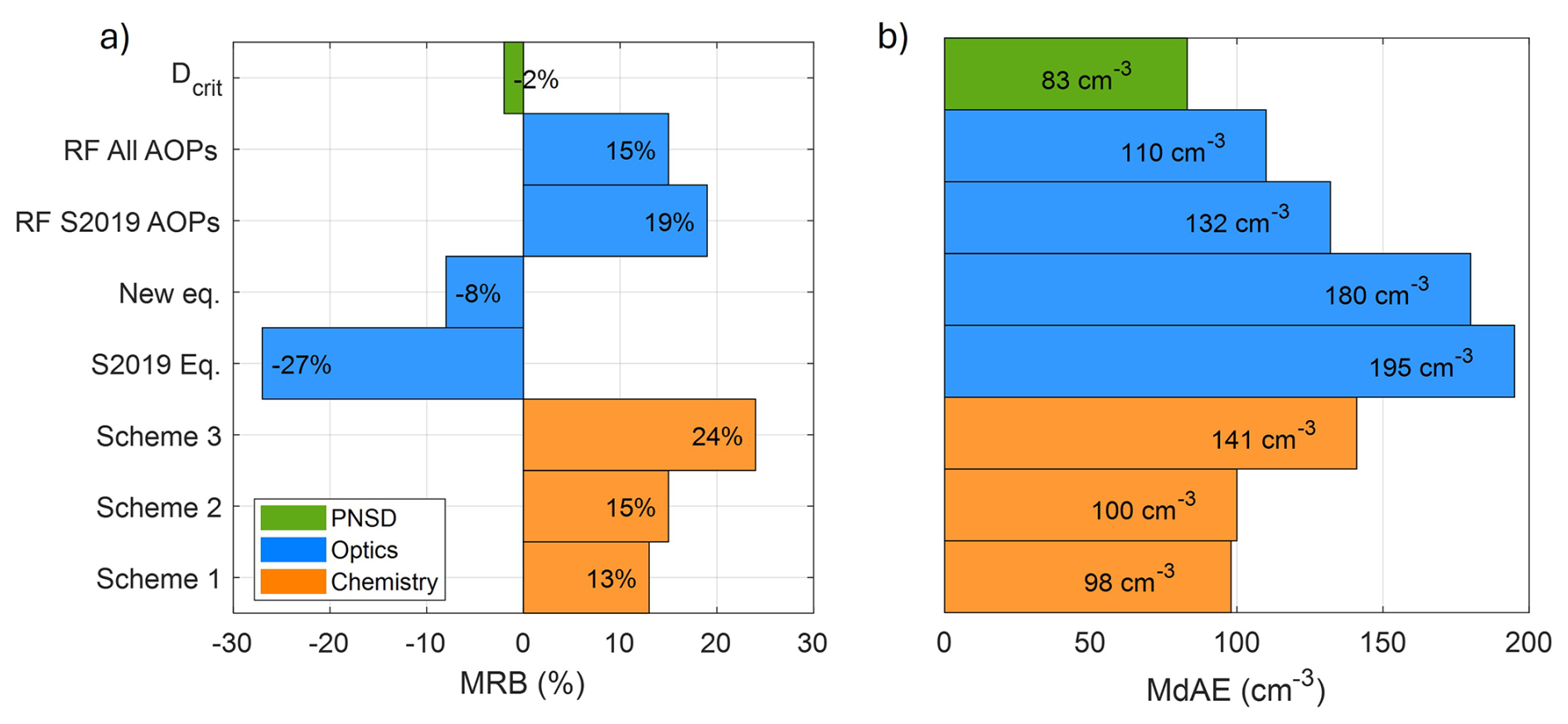
Figure 11 Performance of different CCN prediction methods across all SS and sites. (a) Median relative bias (MRB, %) and (b) median absolute error (MdAE, cm⁻³) between predicted and measured N_CCN. Each box corresponds to a different predictive method applied to the sites with available data.

The AOP-based empirical methods (blue bars S2019 Eq. and New eq.) exhibit larger absolute errors than the PNSD- and chemistry-based approaches. The original S2019 equation substantially underestimates CCN concentrations (MRB =−27 %) and shows a relatively large MdAE (195 cm⁻³). The updated parameterization notably reduces the systematic bias (MRB =−8 %) while maintaining a similar MdAE (180 cm⁻³), indicating improved agreement on average but comparable error dispersion. Despite their lower precision, these approaches are straightforward to implement and only require nephelometer measurements, which greatly enhances their applicability to long-term and globally distributed datasets.

The RF approach represents a further step toward exploiting aerosol optical information. When using the three S2019 AOPs as predictors (σ_sp, BSF, SAE), the RF model shows moderate overprediction (MRB =19 %) and a MdAE of 132 cm⁻³. Incorporating all AOPs (σ_sp, BSF, SAE, σ_ap, AAE, SSA) reduces both bias (MRB =15 %) and MdAE (110 cm⁻³), yielding the lowest overall error dispersion among all AOP-based methods. Although the RF approach does not outperform the D_crit method in terms of bias, it achieves a level of precision comparable to chemistry-based schemes while relying exclusively on optical measurements. In addition, the RF approach provides additional insights into the relative importance of different optical properties for predicting C and k, which cannot be obtained with other methods based solely on optical measurements.

Figure 12 Summary of CCN prediction methods evaluated in this study and recommended use.

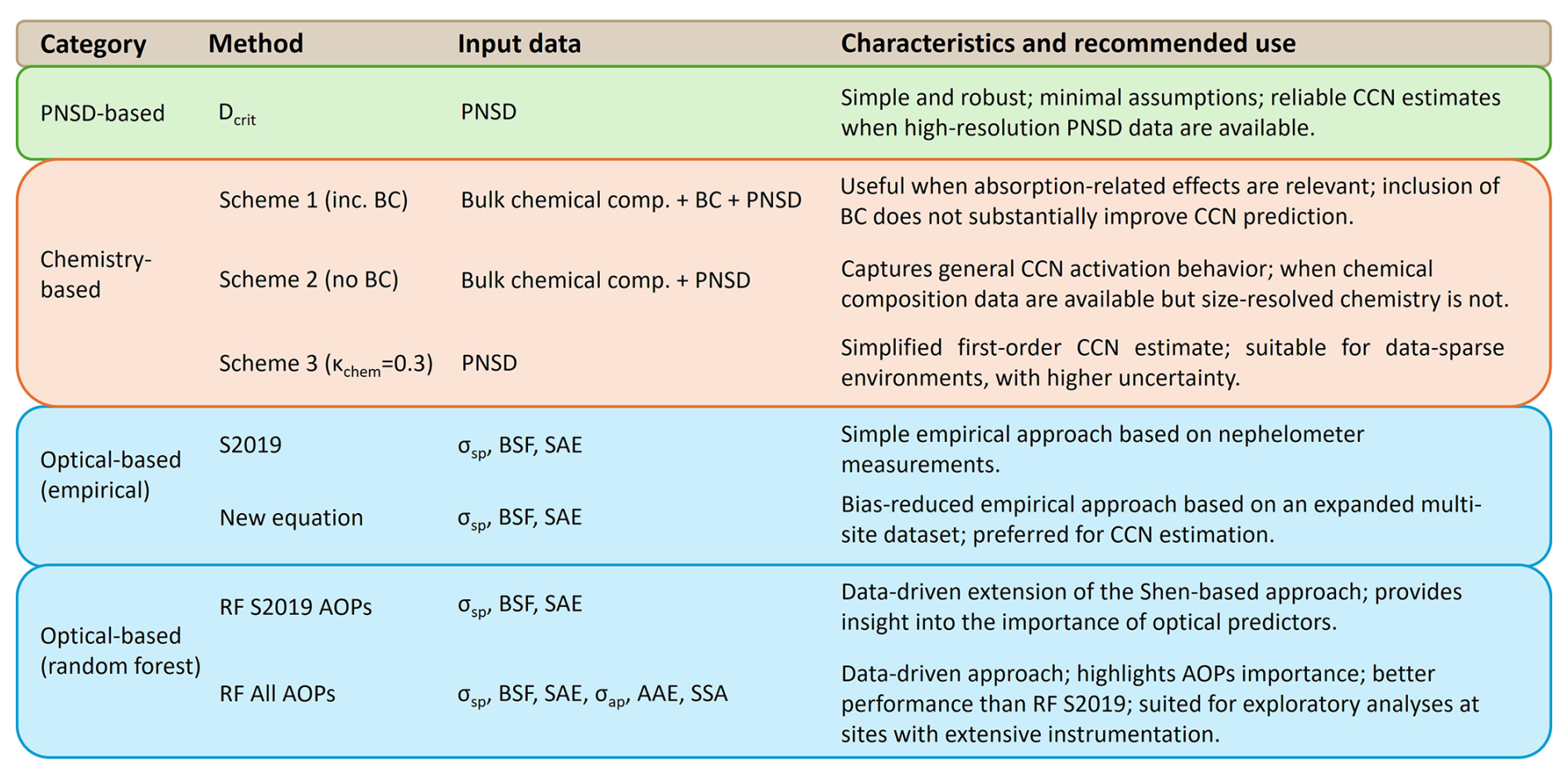
Overall, the different CCN prediction approaches evaluated in this study exhibit complementary strengths in terms of bias and precision. When PNSD data are available, the D_crit method is a robust and straightforward option that minimizes systematic bias. When only nephelometer/optical data are available, the new version of the Shen-based equation or the RF model are preferred, with the former being the simplest to apply and the latter offering improved precision and providing additional insight into the relative importance of individual aerosol optical properties. This makes it particularly valuable for diagnostic and exploratory analyses.

There are still many ways in which the CCN prediction schemes based on aerosol optical or chemical properties can be expanded. For example, Wang et al. (2025b) showed that using dry scattering measurements enhances CCN estimates, while datasets with co-located scattering-related hygroscopicity, f(RH), such as those compiled by Burgos et al. (2019), provide valuable information to refine CCN prediction models under ambient humidity and reduce associated uncertainties. Beyond the 9 sites considered in this study, additional co-located datasets could be combined to harmonize measurements across more locations. In this context, the RF model and the new developed S2019 equation could be applied to long-term aerosol optical records to estimate CCN concentrations over broader spatial and temporal scales and to evaluate the performance of global models (Fanourgakis et al., 2019).

5 Conclusions

This work presents a comprehensive phenomenological study of in-situ aerosol microphysical, CCN activation, chemical composition, and optical properties at 9 surface sites across diverse environments. Several CCN prediction methods using the chemical composition and aerosol optical properties were evaluated.

Analysis of aerosol microphysical properties and CCN activation at 0.4 %  SS reveals a wide variability between environments. The polar and marine sites exhibited the lowest concentrations of N_tot and N_CCN, with values below 400 and 160 cm⁻³, respectively. Despite similar particle concentrations at these remote sites, the significant variability in D_crit and AF underscores the importance of size distribution and chemistry in CCN activation. In contrast, continental sites exhibited the highest N_tot and N_CCN (>2000 and 659 cm⁻³, respectively) with fairly similar AF values (0.25–0.38) and a relatively narrow range in D_crit (76–98 nm). The mountain sites were more similar to the continental sites than the remote sites in terms of aerosol concentrations, but generally exhibited lower AF (<0.24).

The chemical composition analysis of the sites with ACSM measurements shows that organics dominate in continental and mountain sites (50 %–73 % of PM₁), while the marine station is sulfate-rich (35 % of PM₁). Total PM₁ mass ranges from 0.54 to 5.5 µg m⁻³ across sites. Ammonium and nitrate reflect local emissions at the sites and BC is a minor fraction (<9 %) of the aerosol mass. A κ_chem analysis was performed using three different schemes to represent hygroscopcity (κ_chem calculated from ACSM composition + BC, κ_chem calculated from ACSM composition only and fixed κ_chem=0.3). The median hygroscopicity across sites ranged from approximately 0.2 to 0.5 and increased systematically as the organic fraction decreased.

Aerosol optical properties across the seven sites reveal clear environmental differences. Both σ_sp and σ_ap vary with aerosol loading and sources, with continental sites having the highest absorption due to biomass burning and anthropogenic emissions. At the marine site ENA, high σ_sp reflects the presence of marine aerosols with high scattering efficiency. BSF and SAE indicate a predominance of fine particles at continental and mountain sites, whereas marine and polar sites are dominated by coarser particles. AAE values remain generally consistent across sites with median values of approximately 1.2, indicating that BC is the primary absorbing component. Most sites are dominated by scattering aerosols (SSA > 0.9), with lower SSA observed at the site with the most urban influence.

The joint dataset of CCN, aerosol chemical composition and optical properties have been used to evaluate the ability of different prediction methods to estimate CCN concentrations, using either particle number size distribution, chemical composition or aerosol optical properties as inputs. Comparing these prediction methods across site types provides a better understanding of biases and uncertainty in CCN concentration estimates when direct CCN measurements are unavailable. The practical outcome of the different methods is summarized in Fig. 12, which links each approach to the type of available measurements and highlights their complementary strengths. When high-resolution particle number size distribution measurements are available, the PNSD-based approach is the most robust, while chemistry-based schemes offer physically consistent alternatives, though including BC yields limited improvement. Optical-based methods, including the new version of the S2019 equation and the random forest model, provide robust CCN predictions and can be applied at sites with limited measurements. Overall, method selection should balance data availability, predictive accuracy, and interpretability, considering associated uncertainties.

Additionally, the random forest approach allows identifying input variable importance. The application of the random forest (RF) model extended the range of aerosol optical properties considered beyond those included in previous parameterizations. To our knowledge, this is the first explicit use of the absorption Ångström exponent (AAE) as a predictor for CCN estimation based on optical data. RF analysis indicated the importance of AAE in predicting the Twomey exponent k, highlighting the potential value of including absorbing aerosol characteristics in future parameterizations.

Both empirical (Shen-based) and machine-learning (RF) approaches offer practical pathways to estimate long-term CCN trends at stations with extensive aerosol optical property archives. Retrospective application of these methods can provide insights into the evolution of aerosol-cloud interactions over recent decades. A key requirement for such analyses is robust quantification of prediction uncertainties to ensure reliable trend interpretation.

Finally, while this study adds to the accumulated knowledge and previous synthesis of data (e.g., Schmale et al., 2018) relevant for CCN analysis, there are still gaps in spatial coverage. Other observational sites making PNSD and CCN measurements do exist. A truly global CCN climatology, similar in spirit to the effort of Rose et al. (2021) for N_tot and PNSD, would require an extensive harmonization of disparate datasets – it would be a monumental but valuable undertaking.