The impact of rocket-emitted chlorine on stratospheric ozone

Although stratospheric ozone is recovering under the Montreal Protocol, the rapidly expanding space industry may influence the pace of this recovery. We assess the potential for rocket-emitted chlorine, under various launch growth scenarios, to offset the decline in chlorine from regulated Ozone Depleting Substances (ODSs). We use the Whole Atmosphere Community Climate Model (WACCM6) nudged to meteorological reanalyses to simulate realistic atmospheric variability. A modest (times ten) increase in chlorine emissions from rocket launches relative to 2019 causes a near-global column ozone loss of less than 0.1 Dobson Unit (DU) (0.04 %), while a large (times 52) increase leads to 0.6 DU (0.23 %) depletion. Local ozone decreases reach 0.4 % and 2 %, respectively, in the upper stratosphere for these scenarios. Column losses peak at high latitudes, with strong seasonality and meteorology-driven variability in the Arctic. The impact peaks in October in the Antarctic (0.5 and 3 DU depletion for × 10 and × 52 cases), and in April in the Arctic (generally up to 2 DU for the × 52 case, or greater than 8 DU in cold years with meteorology such as 2010/11). Ozone depletion throughout the stratosphere scales linearly with chlorine enhancement. Overall, while the effects of rocket-emitted chlorine under plausible growth scenarios are small, they could partially offset the gains achieved by the Montreal Protocol and should be considered in future assessments of rocket propulsion systems and ozone layer recovery projections.

1 Introduction

The space industry is currently expanding rapidly, especially for commercial use (Dallas et al., 2020). As a result, new spaceports and launch vehicle companies are being established in historically aeronautically active nations such as the United States and Russia, and in nations with emerging space sectors such as China and India. In 2021, commercial space flights by Virgin Galactic, Blue Origin, and SpaceX demonstrated that space tourism is plausible (Ryan et al., 2022), though the future scale of this nascent industry is uncertain. This rapid growth needs to be accompanied by a detailed understanding of the potential environmental impact of the space industry, including the impact of launch-rocket emissions on the ozone layer and climate.

Stratospheric ozone depletion has been a major environmental issue of the past few decades, since the suggestion in the 1970s that chlorine from chlorofluorocarbons (CFCs) could deplete ozone at 40 km (Stolarski and Cicerone, 1974), and especially since the discovery of the Antarctic ozone hole in the 1980s (Farman et al., 1985). The Montreal Protocol on ozone-depleting substances (ODSs) was signed in 1987 and ratified 2 years later. With several subsequent amendments, the Protocol now limits the production and consumption of all major long-lived ODSs ultimately emitted to the atmosphere (Chipperfield and Bekki, 2024). This has resulted in a turnround in stratospheric chlorine (and bromine) levels and signs of ozone recovery have been detected in the upper (Steinbrecht et al., 2017) and polar lower (Solomon et al., 2016) stratosphere. Based on the projected decrease in halogen loadings, models predict that the date when stratospheric ozone values will return to 1980 levels will occur around the mid-late 21st century (Chipperfield et al., 2018). However, other pollution sources, including rocket launches, may affect the rate and extent of this recovery. As the number of national and private space organizations continues to grow, and as the cost of space travel declines, the frequency of rocket launches is expected to rise significantly. This increased activity could make ozone depletion from space launches a serious environmental challenge, as highlighted by Ross et al. (2009). Understanding the impact of rocket engine combustion emissions and exhaust on ozone depletion is essential, as these emissions are injected directly into the atmosphere, including the altitudes of the stratospheric ozone layer.

Rockets can be fuelled by a range of different propellants, which may affect the ozone layer in distinct ways. The pollutants produced by rocket emissions depend on the type of fuel used. For decades, solid propellants have played a fundamental role and have been widely used in the aerospace industry. Solid rocket motors (SRMs), consist of solid aluminium fuel with an ammonium perchlorate (NH₄ClO₄) oxidiser with some also containing hydrocarbons. The benefits of SRMs include easy storability, high reliability, and design simplicity. However, once ignited, they cannot be turned off and are therefore typically used only in the first stage of launch vehicles. The exhaust from SRMs contains a number of compounds of environmental concern, in particular hydrochloric acid (HCl) and alumina particles. As a pollutant emitted by rockets, reactive chlorine could enhance the ozone-depleting catalytic cycles active in the upper stratosphere and polar regions.

Many studies have examined the effects of rocket fuel emissions or single-species impacts, often focusing on emissions from a limited number of injection sites (Danilin et al., 2001b, a; Maloney et al., 2022; Popp et al., 2002; Ross et al., 2004, 2009; Prather et al., 1990; Voigt et al., 2013). Both reactive chlorine and alumina particulates are emitted together in SRM exhaust wakes, compounding the ozone losses that occur (Danilin et al., 2001a). Ryan et al. (2022) used information on 2019 rocket launches and re-entry events to investigate the impacts of multiple rocket-emitted pollutants on stratospheric ozone, including NO_x. They found that ablative NO_x production during re-entry can have a significant effect on stratospheric ozone, while NO_x emissions from launches were relatively less important. The ozone impacts reported in their study were most pronounced in the upper stratosphere. For launch scenarios considering re‐entry NO_x production, a 0.5 % loss of global average column ozone has been estimated, with polar losses exceeding 2 % (Larson et al., 2017). In a recent modelling study, persistent levels of black carbon were calculated after 4–6 years of rocket launch activity, with year‐round ozone loss of 5–15 DU in the Northern Hemisphere (NH) and a potentially more severe Antarctic ozone hole (Maloney et al., 2022). To support such impact studies, rocket emission inventories have been developed, encompassing a wide range of pollutants – including chlorine, NO_x, H₂O, CO₂, black carbon, and alumina – resulting from worldwide rocket launches (Brown et al., 2024a; Ryan et al., 2022).

Recently, Revell et al. (2025) used the SOCOL coupled chemistry-climate model (CCM) in free-running mode in a series of 25-year timeslice experiments (following 10 years of spin-up) to study the possible impact of near-future rocket launches on the ozone layer. They investigated two scenarios for the year 2030 of increased emissions relative to their benchmark 2019 inventory (Brown et al., 2024b) of 97 launches per year: an “ambitious” scenario with 2040 launches per year (× 21 increase on 2019), and a “conservative” one with 884 launches per year (× 9). They found decreases of 0.17 % and 0.29 % in the near-global annual mean ozone abundance under the conservative and ambitious scenarios, respectively. The ambitious scenario produced up to 3 % depletion in the upper stratosphere. Ozone changes in the lower stratosphere were largely not statistically significant compared to the CCM variability, with the notable exception of a large 3.9 % additional depletion in the Antarctic (60–90° S) spring (September–October–November mean). Revell et al. (2025) diagnosed that the rocket-induced ozone depletion was mainly due to chemical loss from the emitted chlorine, and circulation changes due to heating by black carbon particles. For reference, their ambitious scenario of 884 launches per year resulted in annual emissions of 10.13 Gg chlorine, thereby increasing the modelled upper stratospheric volume mixing ratio of inorganic chlorine (Cl_y) by around 0.2 parts per billion (ppbv).

In this paper, we use the Whole Atmosphere Community Climate Model Version 6 (WACCM6) (Gettelman and Rood, 2016) to assess and quantify the impact on ozone from the potential injection of Cl_x from a rocket emission inventory (Brown et al., 2024b). We aim to extend on the work of Revell et al. (2025) by investigating the impact of rocket-emitted Cl_x under a range of scenarios and in a model constrained (by nudging) to have realistic polar meteorology. This is important for quantifying polar ozone depletion and its interannual variability, and reduces the limitations when comparing model simulations with small differences in forcing. Other species, including NO_x, have different sources, chemistry, and spatial–temporal patterns of impact. Adding them to the same sensitivity experiments would make it harder to attribute ozone changes and to isolate the effect of SRM chlorine. The roles of Cl_x and NO_x also vary with altitude, latitude, and season. This study focuses on the polar lower stratosphere, where chlorine activation on polar stratospheric clouds (PSCs) drives ozone loss and where SRM chlorine will likely have a stronger impact. Section 2 describes our setup of WACCM6. Section 3 presents our results for long-term global mean impacts of the rocket emissions and the dependence on variability in polar meteorology. Our conclusions are summarised in Sect. 4.

2 Rocket Emissions and Chemistry-Climate Model

We use the rocket emission inventory of Brown et al. (2024b), which is based on 97 successful rocket launches in the year 2019 from 18 active launch sites located at latitudes between 30° S and 62.9° N. The inventory is compiled from reports from governments and companies and provides the emission mass of H₂O, CO₂, NO_x, Cl_x, BC and Al₂O₃. Here we consider only Cl_x emissions from solid rocket motors, and do not include other rocket-emitted species. The majority of launches with this fuel in 2019 occurred at low latitudes, in particular from Kourou (5.2° N, 307.3° E). In our model simulations we scale the 2019 inventory emissions and apply the emissions each year during the model run (see Table 1).

Brown et al. (2024b)

Table 1 Summary of WACCM simulations with varying rocket Cl_x emissions.

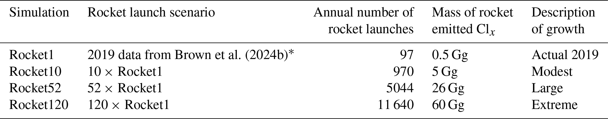
^∗ 2019 inventory of 65 vehicles from 11 launcher families and 97 launches.

We have performed a series of experiments with WACCM6 (Gettelman et al., 2019) which extends from the Earth's surface to around 140 km. All simulations use 88 vertical levels within this domain and a horizontal resolution of 1.9° latitude × 2.5° longtitude. The model includes chemical mechanisms for the simplified tropospheric chemistry with detailed middle atmospheric chemistry (WACCM6 – MA), including heterogeneous reactions on sulfate aerosols and PSCs.

WACCM is very well established and widely used in the international community (e.g. Solomon et al., 2016; Eyring et al., 2016; Gettelman et al., 2019). Several previous studies have shown that WACCM6-SD can well characterise the spatial distribution, vertical profile, and interannual variability driven by dynamical and chemical processes in the Arctic and Antarctic stratosphere, and these studies have evaluated model performance by using satellite observations (e.g. Cuevas et al., 2022; Zhu et al., 2023; Zhang et al., 2024).

The chemical species within WACCM6 include the extended O_x, NO_y, HO_x, Cl_y, and Br_y chemical families, along with CH₄ and its degradation products. In addition to CH₄, we also include N₂O (major source of NO_x), H₂O (major source of HO_x), plus various natural and anthropogenic precursors of the Cl_y and Br_y families. This mechanism also includes primary non-methane hydrocarbons and related oxygenated organic compounds. The chemical mechanism has evolved from previous versions (e.g, Emmons et al., 2010; Lamarque et al., 2012; Kinnison et al., 2007; Tilmes et al., 2016; Marsh et al., 2013) and now includes a total of 100 species, 312 chemical reactions including 91 photolysis reactions, 19 odd-oxygen reactions, 17 odd-hydrogen reactions, 27 odd-nitrogen reactions, 36 odd-chlorine reactions, 21 odd-bromine reactions, 6 odd-fluorine reactions, 17 organic-halogens reactions, 17 sulfur reactions, 12 C1 reactions, 4 tropospheric aerosol and 17 stratospheric aerosol heterogeneous reactions and 28 ion reactions. The source gases (CO₂, CH₄, N₂O, ODSs) are from the CMIP6 forcing dataset (Meinshausen et al., 2017) (see Supplement, Fig. S1) which is constructed from a combination of direct atmospheric measurements, ice core reconstructions, and industrial emission records. The time-varying sea surface temperature and sea ice coverage (to match the forcing meteorology) are from Hurrell et al. (2008) and Kennedy et al. (2011).

In this study, WACCM is nudged to MERRA-2 reanalyses (Hurrell et al., 2008; Feng et al., 2013; Molod et al., 2015) to ensure that the model simulations have realistic lower stratospheric meteorology, which is important for chlorine-induced polar ozone loss. The nudging is applied only to winds and temperature (Gettelman et al., 2019); the chemical species evolve freely. We performed 4 model simulations (see Table 1). The reference case (Rocket1) included all emission sources and is based on the released WACCM6 with a modal aerosol microphysical model (MAM4) of the Community Earth System Model Version 2 (CESM2.1.5) (Danabasoglu et al., 2020). Simulation Rocket1 also includes annually repeating 2019 rocket Cl_x emissions. The other three sensitivity runs were the same as run Rocket1 but scaled the 2019 rocket Cl_x emissions with different factors of 10, 52 or 120. The × 10, × 52, and × 120 scenarios are sensitivity experiments, not specific projections. They are scaled from the 2019 launch inventory, which provides a consistent reference, before rapid growth, to test ozone response under stronger emissions and to examine the linearity of the impacts. This study does not aim to predict the future of SRMs; rather it focuses on the effect of SRM-derived chlorine when injected into the stratosphere. Polar ozone loss is very sensitive to chlorine under cold conditions, so even a relatively small number of SRM launches may cause a clear signal in the polar lower stratosphere. The largest assumed increases in rocket launches are unrealistic for the near future but allow us to test the sensitivity of model results to different levels of chlorine. As the winds in WACCM are constrained here by nudging, we do not investigate the impact of rocket-emitted black carbon on ozone through changes in circulation.

In each simulation the model was integrated over 22 years using the observed source gas boundary conditions based on CMIP6 (see Fig. S1). The runs were nudged to the MERRA-2 meteorology (Molod et al., 2015) from 1990–2012 to ensure that the simulations experienced a realistic range of meteorological conditions, especially at the poles. This is essential for simulating chlorine-driven polar ozone loss, particularly in the more variable Arctic. The winter of 2010/11 was included because it was an exceptionally cold Arctic winter with near-record ozone depletion (Manney et al., 2011). The first 7 years were treated as spin-up and the model years 1997–2012 were analysed for the impacts of rocket emissions. This length of model run is sufficient for us to diagnose the targetted chlorine impact for a range of polar conditions and reasonable background chlorine loading. Although stratospheric chlorine is decreasing, and will continue to do so, we use differences in our model runs to diagnose the relative impact of additional rocket-based emissions.

3 Results

3.1 Impact on Cl_y distribution

Figure 1 shows the zonal mean distribution of inorganic chlorine (Cl_y = $\mathrm{HCl}+{\mathrm{ClONO}}_{\mathrm{2}}+\mathrm{HOCl}+\mathrm{Cl}+\mathrm{ClO}+\mathrm{2}\times {\mathrm{Cl}}_{\mathrm{2}}{\mathrm{O}}_{\mathrm{2}}+\mathrm{2}\times {\mathrm{Cl}}_{\mathrm{2}}+\mathrm{OClO}+\mathrm{BrCl}$) for the reference experiment Rocket1 averaged over model years 1997–2012, and the differences between this and the equivalent quantity from three different rocket emission scenarios. In the reference experiment (Fig. 1a), stratospheric Cl_y peaks at about 3.3 ppbv above 5 hPa in the equatorial region, and above 30 hPa in the high latitudes. Because the long-lived chlorine source gases are not photolysed in the lower atmosphere, the concentration of Cl_y in the troposphere is negligible. Compared to the reference experiment Rocket1, all other rocket emission scenarios show Cl_y enhancements in the stratosphere (1–∼ 100 hPa) and above (Fig. 1b–d). The rocket emissions mainly occur in the tropics and the local enhancement in the Cl_y profile is clearly seen in this region. However, the Cl_y increase is efficiently transported to higher latitudes of both hemispheres by the Brewer-Dobson circulation. In simulation Rocket10, Cl_y increases by approximately 0.03 ppbv in the stratosphere, demonstrating that even modest (× 10) increases in rocket emissions compared to 2019 levels can perturb the stratospheric chlorine budget. Simulations Rocket52 and Rocket120 show even stronger increases, with the former exceeding 0.15 ppbv and the latter exceeding 0.4 ppbv in the stratosphere. The largest increases in the modelled Cl_y mixing ratio occur above the stratopause due to continuing rocket emissions at these altitudes and the decreasing air density. The simulated increase in chlorine becomes partitioned between the Cl_y species based on the background model chemistry and meteorology. Hence, the increase in Cl_y is dominated by enhanced HCl concentrations, while increases in reactive chlorine, particularly ClO, are also evident at high latitudes in the upper stratosphere (∼ 1–3 hPa).

Figure 1 Latitude-height zonal mean annual mean distribution of total inorganic chlorine Cl_y (ppbv) and the differences between sensitivity simulations and run Rocket1, averaged over model years 1997–2012. (a) Cl_y from run Rocket1. (b) Difference between runs Rocket10 and Rocket1. (c) Difference between Rocket52 and Rocket1. (d) Difference between Rocket120 and Rocket1. The dashed lines indicate the approximate locations of the tropopause and stratopause. Note different colour scales in panels (b)–(d).

3.2 Impact on global ozone

Figure 2 shows the zonal mean distribution of ozone for the reference experiment, and the differences between this and the three rocket emission scenarios (averaged over 1997–2012). In simulation Rocket1, ozone concentrations exhibit the characteristic high mixing ratios in the tropical mid-stratosphere, peaking at approximately 10 parts per million (ppmv) between 10–15 hPa. Peak ozone concentrations gradually decrease with increasing latitude, reaching a minimum of approximately 6 ppmv at the poles. This distribution is due to photochemical production at low latitudes followed by transport to the poles via the Brewer-Dobson circulation.

Figure 2 Latitude-height zonal mean distribution of O₃ (ppmv) and the differences between sensitivity experiments and the reference averaged from 1997–2012. (a) O₃ from run Rocket1. (b) The difference between runs Rocket10 and Rocket1. (c) The difference between runs Rocket52 and Rocket1. (d) The difference between runs Rocket120 and Rocket1. The dashed lines indicate the approximate locations of the tropopause and stratopause. Note different colour scales in panels (b)–(d).

Compared to the reference experiment, all of the additional rocket emission scenarios show an overall decrease in stratospheric ozone, most pronounced (in terms of mixing ratio) in the upper stratosphere followed by the high-latitude lower stratosphere. These are the regions where chlorine chemistry is expected to have an impact on ozone (e.g., Farman et al., 1985; WMO, 2022). The upper stratospheric loss occurs through the catalytic cycle involving ClO + O (Stolarski and Cicerone, 1974), while loss in the polar lower stratosphere occurs through reactions involving ClO + ClO (Molina and Molina, 1987) and ClO + BrO (McElroy and Salawitch, 1986). Note, however, that the simulations also show small increases in O₃ in the tropical mid-low stratosphere at 10–30 hPa. Ozone depletion in the upper stratosphere will cause increased penetration of ultraviolet radiation resulting in some ozone “self-healing” (Haigh and Pyle, 1982), which occurs in the tropical region where the radiation is more intense. In simulation Rocket10, ozone depletion is as large as 30 ppbv (1.6 %), concentrated at altitudes of 1–10 hPa at high latitudes. The simulations Rocket52 and Rocket120 show more substantial ozone reductions in the upper stratosphere, with maximum decreases of over 40 ppbv (2.1 %) and 100 ppbv (5.2 %), respectively. Simulations Rocket52 and Rocket120 also show a clearer signal of the ozone impact, consistent with the clearer signal of Cl_y enhancement (Fig. 1).

Figure 3 Profiles of annual mean O₃ depletion from 1 to 100 hPa for sensitivity simulations compared to Rocket1 averaged over 1997 to 2012 for latitude regions (a) 60–90° S, (b) 60° S–60° N, and (c) 60–90° N.

Figure 3 illustrates the mean impacts on stratospheric ozone profiles (1–100 hPa) due to rocket-emitted chlorine in three latitude regions. Ozone depletion occurs in both the upper and lower stratosphere. In the upper stratosphere, between 5 and 1 hPa, the mean year-round depletion can reach almost 5 % in the polar regions in extreme scenario Rocket120. There is a clear scaling of the magnitude of the depletion due to different Cl_y enhancements which is explored in more detail below. The upper stratospheric ozone depletion in the near-global region is somewhat smaller than at high latitudes but, again, increases with the Cl_y scenario. In the polar lower stratosphere, below about 30 hPa, the year-round impact on ozone is larger in the Antarctic than the Arctic, again increasing with increasing Cl_y.

Figure 4 Mean annual cycle of column ozone (DU) from run Rocket1 for (a) Antarctic and (b) Arctic. Also shown (right-hand y axis) is the 1997–2012 mean annual cycle of ozone depletion from runs Rocket10, Rocket52 and Rocket120 compared to run Rocket1.

Ozone depletion in the polar lower stratosphere exhibits a strong annual cycle linked to the occurrence of cold temperatures and the availability of sunlight. Chlorine plays a key role in this springtime chemical ozone depletion so the impact of chlorine from rocket emissions would be expected to show similar behaviour. The winter polar vortex isolates air at high latitudes and contributes to cold temperatures, promoting the formation of PSCs. Reactions on the surfaces of PSCs convert reservoir Cl_y species into active, ozone-destroying radicals which cause rapid ozone loss when sunlight returns in spring (WMO, 2019). Figure 4 illustrates the mean annual cycle in high-latitude column ozone from run Rocket1, and the impact of the three sensitivity simulations. For the Antarctic run Rocket1 shows a minimum mean ozone column over this extended polar area of near 220 DU in October, at the end of the ozone hole period. This is also the month of the largest impact on column ozone (−7 DU (3.3 %) in run Rocket120). For the Arctic the maximum column of around 400 DU occurs in the springtime (April). This is also the time of the maximum reduction in simulations with substantial chlorine perturbations (runs Rocket52 and Rocket120).

Figure 5 Profiles of monthly mean O₃ depletion (%) from 1 to 100 hPa for sensitivity simulations compared to Rocket1 averaged from 1997 to 2012 for polar regions (a) 60–90° S in October and (b) 60–90° N in April.

We now repeat the analysis of Fig. 3 for the polar regions and months of largest mean depletion in the lower stratosphere, October and April (Fig. 5). Analysis of these months shows the much stronger impact of chlorine in the lower stratosphere in the Antarctic due to the colder and less variable polar meteorology. The extreme run Rocket120 produces an additional 6 % depletion in the Antarctic lower stratosphere in October, compared to a small mean depletion of just under 2 % in the Arctic in April.

3.3 Dependence of additional ozone depletion on chlorine

Figures 2–5 clearly show that the amount of additional ozone depletion from rockets increases with the magnitude of additional Cl_x emitted. Figure 6 quantifies that relationship more fully for annual mean ozone depletion in the near-global upper stratosphere (Fig. 6a) and polar lower stratospheres (Fig. 6b and c). In these regions the additional ozone loss depends linearly on chlorine. In the upper stratosphere the additional loss of 2.2 % in run Rocket120 is caused by 0.32 ppbv additional Cl_y from a scenario of × 120 the 2019 rocket inventory, i.e. a slope of 6.9 % ppbv⁻¹ Cl or 0.02 % loss per additional increase in inventory. For the polar regions the slopes in annual mean ozone loss versus Cl_y are also linear, with a larger slope in the Antarctic than the Arctic. We also show the polar results for the months of maximum impact (see Fig. 4). The maximum lower stratospheric impact occurs in September in run Rocket120 with a 5 % depletion for an additional 0.13 ppbv Cl_y in the × 120 scenario, i.e. 38 % ppbv⁻¹ Cl or 0.04 % loss per additional increase in 2019 inventory. The impact of scenarios not simulated here can simply be interpolated from the linear plots for perturbations smaller than run Rocket120.

Figure 6 Correlation of mean ozone depletion (%) versus increase in Cl_y (ppbv) from model sensitivity simulations compared to Rocket1 averaged over 1997 to 2012 for regions (a) near-global (60° S–60° N) 40 km annual mean, (b) Arctic (60° N–90° N) 20 km annual mean and April, and (c) Antarctic (60° S–90° S) 20 km annual mean and October. Note different x-axis scale in panel (a) and y-axis scale in panel (c).

3.4 Impact of interannual meteorological variability

Springtime polar ozone depletion exhibits strong interannual variability, especially in the NH. A strong motivation for running WACCM in the nudged mode was to create simulations with realistic stratospheric polar meteorology. Figure 7 shows the long-term seasonal variation of the total ozone column. This highlights the latitude dependence of the chlorine impact and, especially, the significant seasonal depletion in the polar regions. The observation-based MERRA-2 reanalyses (Fig. 7a) demonstrate the observed annual cycles and interannual variability which is generally well captured by WACCM (Fig. 7b and c, see also Fig. S2). In simulation Rocket1, the ozone column shows the expected spatial and temporal pattern: in the tropics (30° S–30° N), the column remains between 280–350 DU throughout the year, with little variation; in the mid-latitudes (30–60° N/S), it is generally higher, reaching 350–420 DU, and shows a clear seasonal cycle; the polar regions fluctuate most dramatically, with column ozone dropping sharply in the Antarctic in spring (September–October), reaching a minimum of nearly 200 DU, corresponding to a typical ozone hole event, while the Arctic also experiences a certain degree of ozone depletion in spring (March–April). The impact of polar meteorology is evident through the small Antarctic ozone depletion in the disturbed year of 2002 (Feng et al., 2005), and the smaller Arctic columns in the cold winter/springs of 1996/97, 1999/2000 and 2010/11 (Chipperfield et al., 2015).

Figure 7 (a) Observation-based total column O₃ (DU) for 1997–2012 from MERRA-2 reanalyses. (b) Difference in column ozone between model control run (without rocket emissions) and panel (a). (c) Latitude-time variation of total column O₃ (DU) for 1997–2012 from run Rocket1. Panels (d)–(f) show the differences in column ozone with respect to Rocket1 for simulations (d) Rocket10, (e) Rocket52 and (f) Rocket120. Note different colour scales in panels (d)–(f).

Figure 8 Mean annual magnitude of polar ozone depletion (DU) for 1997–2012 meteorological years for 3 rocket emission scenarios for (a) Antarctic (60–90° S) and (b) Arctic (60–90° N) regions. Also shown as shading on each line is the range of ozone depletion, indicating the minimum and maximum monthly values over each year.

Compared to the control run, all rocket emission scenarios show ozone reductions at high latitudes (Fig. 7d–f). We have computed the decrease in polar column ozone for model years 1997–2012 for selected emission scenarios (Fig. 8). In the Antarctic (90–60° S), the depletion under the Rocket10 scenario is around 0.5 DU (0.12 %), for Rocket52 it is 2.5 to 3 DU (0.6 % to 0.7 %), while Rocket120 reaches 6 to 8 DU (1.4 % to 1.7 %). In the Arctic (60–90° N), the interannual variability of ozone depletion is more pronounced, with the scenario Rocket10 showing only 0.3 to 0.5 DU (0.04 % to 0.06 %), Rocket52 giving 1.5 to 3 DU (0.2 % to 0.4 %), and Rocket120 reaching 4 to 7 DU (0.5 % to 0.84 %). In particular, in the year 2011 Arctic loss exceeds 7.5 DU (0.9 %), corresponding to a year of extreme cold and a stable polar vortex, showing that Arctic ozone can be more sensitive to rocket chlorine emissions under specific meteorological conditions. Generally, the Antarctic displays a large, stable signal of ozone depletion, while the Arctic shows considerable interannual differences. Notably this variability can cause Arctic springtime loss (in absolute terms) to exceed Antarctic loss in extreme years.

Figure 9 Distribution of Antarctic total column O₃ (DU) in September and October and the differences between sensitivity experiments and reference simulation from 1997–2012. (a) O₃ in reference case Rocket1. (b) The difference between simulations Rocket10 and Rocket1. (c) The difference between simulations Rocket52 and Rocket1. (d) The difference between simulations Rocket120 and Rocket1. Note that the contour scales differ between the panels.

A map of the mean ozone depletion in Austral spring (September and October) is shown in Fig. 9. In the reference run Rocket1 (Fig. 9a), the total ozone column in the Antarctic spring exhibits the typical hole distribution, with the lowest values in the core area of the polar vortex less than 180 DU, while the surrounding collar areas reach 300–340 DU. The overall spatial distribution is consistent with the observed Antarctic ozone hole (not shown), indicating that the nudged WACCM6 model reproduces well the seasonal evolution of ozone in polar regions. Compared to the reference experiment, all rocket emission scenarios lead to a decrease in Antarctic column ozone and, as expected, the reduction increases with the amount of emissions (Fig. 9b–d). In the scenario Rocket10, the maximum decrease in column ozone in the polar region is about 0.5 DU at the edge of the polar vortex; in the scenario Rocket52, ozone loss is substantially larger, with a maximum reduction of 3 DU at the vortex edge; in the Rocket120 scenario, the decline in polar ozone is larger still, and reaches 7 DU. This shows that that polar spring ozone is sensitive to additional chlorine sources. Overall, however, this result indicates that even large increases in chlorine-fuelled rocket launches compared to 2019 (Rocket10) is sufficient to cause only modest losses in polar spring ozone although this will offset to some extent the recovery of the Antarctic ozone hole.

Figure 10 Distribution of Antarctic total column O₃ (DU) and the differences between sensitivity experiments and reference simulation for October 2011. (a) O₃ in reference case. (b) The difference between simulations Rocket10 and Rocket1. (c) The difference between simulations Rocket52 and Rocket1. (d) The difference between simulations Rocket120 and Rocket1. Note that the contour scales differ among the panels.

We can use the model results to investigate the impact of the rocket emissions on Antarctic ozone in specific years. Figure 10 shows the column ozone impact for October 2011, a year of relatively large depletion within the small variability of Antarctic ozone (Fig. 6). The column loss is slightly larger than for the long-term-mean results of Fig. 9.

Figure 11 Distribution of Arctic total column O₃ and the differences between sensitivity experiments and reference simulation for April 2011. (a) Column O₃ from reference case. (b) The difference between Rocket10 and Rocket1. (c) The difference between Rocket52 and Rocket1. (d) The difference between Rocket120 and Rocket1. Note the different colour scales in panels (b)–(d).

For the Arctic, stratospheric ozone depletion exhibits clear interannual variability and the strongest ozone depletion modelled here occurred in 2011 (Fig. 8). The extreme cold atmosphere in winter 2010/11 promoted the formation of PSCs and enhanced the springtime chlorine-driven chemical loss of ozone depletion (Manney et al., 2011). Figure 11 shows that the simulated Arctic ozone minimum (Fig. 11a) is around 239 DU total column ozone which is consistent with observations (Manney et al., 2011). In contrast to the Antarctic with maximum loss at the vortex edge, this cold Arctic winter results in the maximum impact at the centre of the disturbed vortex. Moreover, the column ozone depletion under these conditions (0.9, 5.5 and 13 DU for runs Rocket10, Rocket52 and Rocket120, respectively) is much larger (almost double) the largest depletion in the Antarctic. When averaged over 90-60° latitude the depletion is, however, similar (Fig. 8).

4 Discussion

A motivation for this study was to further investigate the impact on ozone of rocket-emitted chlorine presented by Revell et al. (2025). We now quantitatively compare our results with that study. For reference, the annual 2019 stratospheric emissions of chlorine in the inventory of Brown et al. (2024b), as processed in our WACCM simulations, is 0.5 Gg yr⁻¹. This is 16 % of the overall rocket emissions from 97 launches in that year. Assuming a 5-year stratospheric residence time of these emissions, the mean increase in Cl_y volume mixing ratio from continuous release of these emissions would be around 2.8 parts per trillion (pptv). The peak in stratospheric chlorine loading in the mid-late 1990s was about 3600 pptv, of which around 3000 pptv was contributed by ODSs (Dubé et al., 2025).

Revell et al. (2025) reported decreases of 0.17 % and 0.29 % in the near-global (60° S–60° N) annual mean column ozone abundance under their conservative (884 launches per year) and ambitious (2040 launches per year) scenarios, respectively. They also reported 3.9 % depletion in Antarctic (60–90° S) springtime (September–October–November mean) column ozone. These reductions can be compared with observations of ozone changes over the past few decades. WMO (2022) reported that the current (2017–2020) total column ozone was about 2.3 % below the 1964–1980 reference mean in the near-global average, about 1.1 % below the reference mean in the tropics (20° S–20° N), and about 3.6 % and 4.7 % below the reference means in NH and SH mid-latitudes (35–60° latitude), respectively.

Revell et al. (2025)

Table 2 Summary of ozone depletion (DU (and %)) under different scenarios in this work (compared to Rocket1) and Revell et al. (2025).

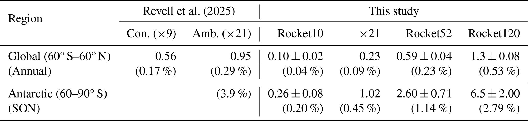
The results of Revell et al. (2025) are summarised in Table 2, along with the equivalent quantities from our WACCM sensitivity runs compared to the reference run Rocket1. For near-global column ozone we find decreases of 0.04 %, 0.59 % and 1.3 % from runs Rocket10, Rocket52 and Rocket120, respectively. The decreases in Antarctic SON column ozone from the same runs are 0.20 %, 1.14 % and 2.79 %. Although we did not perform identical simulations to Revell et al. (2025), our Rocket10 simulation is similar to their conservative scenario and we can use the derived sensitivity of our simulations to Cl (see Fig. 6) to estimate the WACCM results for their ambitious (× 21) case. Overall we derive substantially smaller ozone depletion than Revell et al. (2025), for example 0.09 % for global ozone and 0.45 % for SON Antarctic ozone from an “ambitious” scenario. It should be noted that we are only deriving the impact of the chlorine emissions, while Revell et al. (2025) included the effects of other emissions, notably the impact of black carbon on circulation. Revell et al. (2025) also constructed a specific scenario of future rocket launches which caused chlorine emissions at different locations to those assumed in our simplified scaling. Nevertheless, the differences between the model simulations are large since chlorine, which is transported globally by the Brewer-Dobson circulation, appears to be responsible for the majority of the chemical ozone depletion. It seems that the differences between our simulations are at least partly due to the magnitude of the modelled chlorine perturbations from the rocket emissions. For a given rocket scenario we find a smaller increase in Cl_y than Revell et al. (2025). For example, they show increases in stratospheric Cl_y of around 0.2 ppbv from their ambitious run (their Fig. 3c), while we see smaller increases even from our Rocket52 simulation (Fig. 1). This is despite their ambitious scenario emitting 10.13 Gg of chlorine into the stratosphere per year, while a × 21 scenario in our WACCM setup would emit 21 × 0.5 = 10.5 Gg yr⁻¹, a similar amount.

The smaller Cl_y response simulated here compared to Revell et al. (2025) may reflect differences in detail of the location of the rocket emissions and the stratospheric circulation in the respective models. For example, the spread of the emissions through the stratosphere by the slow Brewer-Dobson circulation, and thus their residence time in the stratosphere, will depend on the circulation which can vary between models. Further diagnosis of this is beyond the scope of this paper and would need formal model-model intercomparisons.

5 Conclusions

We have used a detailed CCM (WACCM6) to study the potential impact of rocket-emitted chlorine on stratospheric ozone. In particular, we have investigated the potential for future increased numbers of rocket launches, fuelled by solid propellants, to offset recovery of the ozone layer from the effects of ODSs. The CCM is nudged towards meteorological reanalyses from 1990–2012 to achieve realistic lower stratospheric meteorology, in order to allow accurate quantification of small differences in the model experiments. Different scenarios for the number of annual rocket launches are obtained by scaling a reference 2019 inventory (Brown et al., 2024b).

Lower stratospheric ozone loss and column depletion are largest at high latitudes with a pronounced annual cycle and, in the Arctic, large meteorology-driven variability. The impact on Antarctic ozone peaks in October (additional depletion of 0.5 DU (modest growth in launches) and 3 DU (large growth)), while the impact in the Arctic peaks in April (2 DU for large growth). Although the mean impact in the Arctic is much smaller than for the Antarctic, the ozone loss shows large variability. In very cold years (e.g. exemplified by 2010/11 meteorology), the column loss in the Arctic exceeds the Antarctic for all launch scenarios and can exceed 8 DU for large growth. Ozone depletion in both the polar lower stratosphere and upper stratosphere shows a clear linear dependence on the level of chlorine enhancement.

Overall, the estimated impact of rocket-emitted chlorine for reasonable growth scenarios is small but does have the potential to offset some of the gains of the Montreal Protocol. However, we find a smaller impact than the recent study of Revell et al. (2025), possibly at least in part due to different increases in stratospheric chlorine loading from similar emission scenarios. The potential impact of chlorine needs to be considered when deciding on propulsion systems for future rocket launches and in projections of ozone layer recovery.