Measurement report: Observational analysis of mode-dependent fog droplet size distribution evolution and improved parameterization using segmented gamma and lognormal fitting

Fog droplet size distributions (DSDs) evolve under the influence of many physical processes, yet their development through the fog lifecycle remains insufficiently understood and challenging to represent in numerical models, constraining the accuracy of fog forecasting. To improve understanding of the fog evolution, field observations under a polluted background were conducted during winters from 2006–2009 and 2017–2018 in Nanjing, China. Among the 27 observed fog events, microphysical properties including fog droplet number concentration (N_f), liquid water content (LWC), volume-mean radius (R_v), and effective radius (R_eff) varied substantially. Unimodal, bimodal, and trimodal DSDs were observed, with mode separating diameters of 2 µm for unimodal; 2 and 6–18 µm for bimodal; and 2, 6–12, and 18–26 µm for trimodal DSDs. Both the number of modes and the mode separating diameters vary over the fog life cycle, with more frequent and pronounced changes occurring during fog formation and dissipation or during periods of strong fluctuations in N_f and LWC. Compared with unimodal DSDs, bimodal and trimodal DSDs exhibited broader PDF distributions of LWC, R_v and R_eff. Based on these observational features, segmented gamma and lognormal fits were applied to mean DSDs using partition points at 10 and 20 µm. Comparisons between microphysical parameters derived from the fitted DSD and observations show that three-segment fitting improved estimates of N_f and LWC, while substantially enhanced the representation of R_eff, absorption coefficient, and optical thickness, reducing deviations from up to 90 % to within 20 %.

1 Introduction

Composed of suspended small water droplets or individual ice crystals in the air near the surface, fog has multiple impacts ranging from transportation, vegetation, air quality, human health and economy (Gultepe et al., 2014; Jia et al., 2019; Lakra and Avishek, 2022). Due the sharp decline in visibility, long duration, wide spatial coverage associated with fog, it is essential and urgent to improve fog modelling and forecasting. The formation and evolution of fog is driven by macro and microphysical processes including precipitation, radiation, advection, cloud-base lowering, turbulent, aerosol activation and condensation (Gultepe et al., 2007; Mazoyer et al., 2022; Shao et al., 2023; Wang et al., 2020). With different physical processes interact with each other nonlinearly, fog remains as a challenging problem for numerical weather prediction (NWP), even though progress have been made in recent years (Boutle et al., 2018; Martinet et al., 2020; Tudor, 2010).

In order to gain a better understanding in mechanisms of fog evolution, in situ observations have been conducted worldwide with different regions and aerosol backgrounds (Elias et al., 2009; Gultepe et al., 2007, 2009; Gultepe and Milbrandt, 2007; Haeffelin et al., 2010; Mazoyer et al., 2022). Marked variabilities of microphysical parameters such as fog number concentration (N_f) and liquid water content (LWC) have been found. Fogs in polluted area show higher N_f due to higher aerosol number concentration (N_a), while in relative clean regions including mountains, rainforests and rural areas there are more big droplets, which contribute to LWC significantly (Gultepe and Milbrandt, 2010; Guo et al., 2015; Li et al., 2017; Nelli et al., 2024). Also, the fierce competition for water vapor associated with higher N_a suppresses the condensation growth in urban areas, resulting a lower N_f of large droplets and smaller dispersion in urban fog compared to clean regions (Ge et al., 2024).

Meteorological variables and large-scale processes strongly influence fog formation. In general, fog can be classified into two categories: airmass fog and frontal fog, which can be further divided into cold-advection and warm-advection fog, radiation fog, and sea fog etc. (Willett, 1928). Another fog-forming mechanism is the overall lowering of a cloud layer, including its cloud top (Koračin et al., 2014). Radiation fog typically forms near the surface under clear skies and weak winds associated with anticyclonic conditions. Its primary mechanism is radiative cooling, while opposing effects include upward soil heat flux and the warming and moisture loss caused by turbulent mixing within the stable boundary layer (Brown, 1980; Roach, 1976; Turton and Brown, 1987). The advection fog is associated with the advection of a moist air mass with a temperature contrast relative to the underlying surface, which is mainly coastal but also can be observed over land (Friedlein, 2004). Advection-radiation fog is produced by the radiative cooling of moist air that has been advected inland from the ocean or another large water body (Ryznar, 1977). The C-FOG field campaign along the Atlantic Canada and northeastern US coastlines showed that coastal fog was influenced by multiple weather systems, including northeastern high pressure, west–northwest low pressure, and tropical cyclonic activity (Gultepe et al., 2021). Another study in the region found that fog associated with cyclonic systems was consistently produced by cloud-base lowering and subsequent downward extension to the surface, whereas anticyclonic fog developed either from surface radiative cooling or from the downward extension of low-level stratus to the surface (Dorman et al., 2021).

The fog droplet size distribution is a key characteristic of fog microphysical processes (Niu et al., 2012), which is influenced by aerosol chemical composition and number concentration as well as various environment factors such as temperature, humidity, wind speed and direction (Mazoyer et al., 2017; Price, 2019). Fog droplet size distributions (DSDs) often exhibit one or more distinct modes, referred to as unimodal, bimodal, or trimodal DSD, and can be attributed to different origins of the fog and processes within it (Elias et al., 2015; Hammer et al., 2014; Sampurno Bruijnzeel et al., 2006). Kunkel (1982) finds various shapes in DSDs measured in advection fogs. Many other studies have shown the existence of bimodal DSDs in mature radiation fogs (Meyer et al., 1980; Pinnick et al., 1978; Roach et al., 1976; Wendisch et al., 1998). Gultepe and Milbrandt (2007) reported DSD modes near 4 and 23 µm during winter fog events in the Toronto region. Boudala et al. (2022) investigated the seasonal and microphysical characteristics of fog at Cold Lake Airport in northern Alberta, Canada, and found that radiation fog exhibited a bimodal droplet spectrum with peaks at 4 and 17–25 µm. Mazoyer et al. (2022) observed that fog DSD in a semi-urban area of Paris exhibited both single mode (about 11 µm) and double mode (about 11 and 22 µm). When the fog DSD is bimodal, there is a mass transfer from smaller droplets to larger droplets which may due to collision-coalescence process, while sedimentation by gravity speeds up the removal of fog droplets (Mazoyer et al., 2022). The initial fog DSD is influenced by environmental supersaturation and background aerosol properties. As visibility decreases and fog develops, the DSD broadens, transitioning from unimodal to multimodal (Mazoyer et al., 2022). The characteristics of the DSD also strongly influence the optical properties of fog. Stewart and Essenwanger (1982) showed that the attenuation of electromagnetic radiation by fog depends sensitively on the shape of the droplet size distribution. The DSD and water vapor determine the overall optical properties of fog and its effects on visibility and radiative transfer together.

Integrated with in situ measurement, numerical experiment is a commonly used approach to gain a better understanding of the physical mechanism in fog. Over the past decade, numerous numerical experiments have been conducted to evaluate the fog forecasting capabilities and limitations of various mesoscale NWP models, leading to notable progress (Cui et al., 2019; Payra and Mohan, 2014). Despite WRF has made progress in forecasting certain variables such as temperature and wind, it often struggles to capture the accurate fog lifecycle (Peterka et al., 2024; Román-Cascón et al., 2016). The simulated evolution of fog exhibits a sensitivity to the shape of the DSD comparable to its sensitivity to aerosol loading or cloud droplet number concentration (CDNC), yet it remains one of the least investigated and rarely adjusted components of microphysical parameterization schemes (Boutle et al., 2022). A simulation of a heavy fog event in North China Plain found that effective radius of fog droplet decreases nonlinearly with aerosol number concentration (Jia et al., 2019). Since the effective radius was obtained under the assumption of a monodisperse DSD and the dispersion effect was neglected, it may have been overestimated or underestimated due to fog-aerosol interactions (Chen et al., 2016; Liu and Daum, 2002). Currently, fog DSDs are described using various spectral distribution functions such as exponential, gamma or lognormal functions in bulk and bin microphysical scheme (Kessler, 1969; Khain et al., 2015). However, the fog DSD exhibits strong spatial and temporal variability and evolves throughout the fog lifecycle, often displaying distinct features and deviating from idealized distributions due to turbulent mixing, radiative effects, and gravitational settling (Gultepe et al., 2007; Nelli et al., 2024; Tampieri and Tomasi, 1976; Wang et al., 2021). Such variabilities in DSD could cause substantial deviations from the predefined spectral distribution functions, further bringing challenges for fog parameterization (Khain et al., 2015; Lakra and Avishek, 2022). Therefore, a more physically consistent and adaptable representation of DSD is required to improve simulation reliability of fog evolvement.

In this study, based on the observation data of the 27 fog events obtained in Nanjing, China during the winters of 2006–2009, 2017–2018, we focus on the characteristics and evolution of DSDs, how they are associated with microphysical characteristics and how to improve the representation of multimodal size distributions using the gamma and lognormal function. The rest of the article is organized as follows. Section 2 describes the observation site, data, and methods used in this study. Section 3 presents the results, including an overview of microphysics across 27 fog events, an analysis the fog lifecycle under different modes, the correlations between microphysical characteristics and varying DSD modes, and a refinement of the gamma and lognormal fitting approach with an evaluation of its performance. The main conclusions are presented in Sect. 4.

2 Data set and methods

The field campaign was conducted during the winters of 2006–2009 and 2017–2018, with each campaign lasting approximately one month per year. The sampling site was located in the northwestern suburban area of Nanjing, Jiangsu Province, China (32.2° N, 118.7° E; 22 m above sea level), north of the Yangtze River and surrounded by industrial facilities, residential areas, and major roads (Niu et al., 2010, 2012). The DSD was measured with a fog monitor (FM-100) from Droplet Measurement Technologies (DMT, USA) with diameters ranging from 1 to 50 µm into 20 bins, at a sampling frequency of 1 Hz. The width of each bin is 2 µm for the first 10 bins and 3 µm for the last 10 bins. To exclude the influence of large unactivated aerosol particles, data from the first bin (1–2 µm) are omitted (Lu et al., 2013). Fog with N_f > 10 cm⁻³ and LWC > 10⁻³ g m⁻³ was identified (Lu et al., 2020; Wang et al., 2021). Microphysical characteristics including fog number concentration (N_f), liquid water content (LWC), volume-mean radius (R_v), effective radius (R_eff), relative dispersion (ε), autoconversion threshold (T) and first bin strength (FBS) were calculated through following formulas:

$$\begin{array}{}\text{(1)}& {\displaystyle }{N}_{\mathrm{f}}=\sum n\left(r\right)\text{(2)}& {\displaystyle }\mathrm{LWC}=\mathrm{1}\times {\mathrm{10}}^{-\mathrm{6}}\mathit{\rho }\sum {\displaystyle \frac{\mathrm{4}\mathit{\pi }}{\mathrm{3}}}{r}^{\mathrm{3}}n\left(r\right)\text{(3)}& {\displaystyle }{R}_{\mathrm{v}}={\left({\displaystyle \frac{\sum n\left(r\right)r^{\mathrm{3}}}{N_{\mathrm{f}}}}\right)}^{\frac{\mathrm{1}}{\mathrm{3}}}\text{(4)}& {\displaystyle }{R}_{\mathrm{eff}}={\displaystyle \frac{\sum n\left(r\right)r^{\mathrm{3}}}{\sum n\left(r\right)r^{\mathrm{2}}}}\text{(5)}& {\displaystyle }\mathit{\sigma }={\left({\displaystyle \frac{n\left(r\right){\left(r-\stackrel{\mathrm{‾}}{r}\right)}^{\mathrm{2}}}{N_{\mathrm{f}}}}\right)}^{\frac{\mathrm{1}}{\mathrm{2}}}\text{(6)}& {\displaystyle }\mathit{\epsilon }={\displaystyle \frac{\mathit{\sigma }}{\stackrel{\mathrm{‾}}{r}}}\text{(7)}& {\displaystyle }T={\displaystyle \frac{P}{P_{\mathrm{0}}}}=\left[{\displaystyle \frac{{\int }_{r_{\mathrm{c}}}^{\mathrm{\infty }}{r}^{\mathrm{6}}n\left(r\right)\mathrm{d}r}{{\int }_{\mathrm{0}}^{\mathrm{\infty }}{r}^{\mathrm{6}}n\left(r\right)\mathrm{d}r}}\right]\left[{\displaystyle \frac{{\int }_{r_{\mathrm{c}}}^{\mathrm{\infty }}{r}^{\mathrm{3}}n\left(r\right)\mathrm{d}r}{{\int }_{\mathrm{0}}^{\mathrm{\infty }}{r}^{\mathrm{3}}n\left(r\right)\mathrm{d}r}}\right]\text{(8)}& {\displaystyle }\mathrm{FBS}={\displaystyle \frac{N_{\mathrm{1}\mathrm{st}}}{N_{\mathrm{f}}}}\end{array}$$

where ρ is the density of water, r is the fog droplet radius of each bin, $\stackrel{\mathrm{‾}}{r}$ is the mean arithmetic radius defined with $\stackrel{\mathrm{‾}}{r}=\sum \frac{n\left(r\right)r}{N_{\mathrm{f}}}$, r_c is defined with $r_{\mathrm{c}}\approx \mathrm{4.09}\times {\mathrm{10}}^{-\mathrm{4}}{\mathit{\beta }}_{\mathrm{con}}^{\frac{\mathrm{1}}{\mathrm{6}}}\frac{N^{\frac{\mathrm{1}}{\mathrm{6}}}}{{\mathrm{LWC}}^{\frac{\mathrm{1}}{\mathrm{3}}}}$, in which ${\mathit{\beta }}_{\mathrm{con}}=\mathrm{1.15}\times {\mathrm{10}}^{\mathrm{23}}$, N_1st is the number concentration of the first bin (2–4 µm) following the exclusion of the 1–2 µm bin.

Because visibility observations were unavailable for fog cases 1–3 and 18–20, visibility for these cases was estimated using the observed fog droplet spectra and the microphysical parameterization scheme developed by Gultepe et al. (2006), based on the extinction theory of visible light in fog:

$$\begin{array}{}\text{(9)}& V={\displaystyle \frac{-\ln \mathit{\alpha }}{{\mathit{\beta }}_{\mathrm{ext}}}}\end{array}$$

in which

$$\begin{array}{}\text{(10)}& {\mathit{\beta }}_{\mathrm{ext}}=\mathit{\pi }\sum Q_{\mathrm{ext}}n\left(r\right)r^{\mathrm{2}}\mathrm{d}r\end{array}$$

where α is the constant threshold, typically set to 0.02, β_ext represents the extinction coefficient, Q_ext is the Mie extinction efficiency, which depends on particle radius, number concentration, and the wavelength of visible light. When droplet size exceeds about 4 µm, Q_ext approaches a constant value of 2. For smaller droplets (less than 4 µm), Q_ext varies between 0.9 and 3.8 (Brenguier et al., 2000; Koenig, 1971).

Previous studies have shown that DSDs can exhibit one or multiple modes (Elias et al., 2015; Hammer et al., 2014; Sampurno Bruijnzeel et al., 2006). Therefore, in this study, two approaches were employed to identify the presence of multimodal DSDs and to determine the corresponding number of modes and their mode separating diameters: (1) identifying turning points where the number concentration transitions from decreasing to increasing with droplet size, and (2) determining modes using unimodal and multimodal gamma and lognormal functions. The detailed procedures are described below.

• 1.

  Identify turning points

  For a DSD defined on discrete diameter bins, the change rate of number concentration was first computed as

  $$\begin{array}{}\text{(11)}& \mathrm{\Delta }{n}_i\left(D\right)={\displaystyle \frac{n_i\left(D\right)-n_{i+\mathrm{1}}\left(D\right)}{n_i\left(D\right)}},i=\mathrm{1},\mathrm{2},\mathrm{\dots },\mathrm{19}\end{array}$$

  where  D is the droplet diameter, n(D) is the number concentration for each bin. The sign of Δn_i(D) characterized the local trend of the DSD: a positive value indicates decreasing concentration with increasing diameter, whereas a negative value indicates increasing concentration with increasing diameter. The turning diameter D_turn was identified as the diameter where the sign of Δn_i(D) change from positive to negative, with the additional requirement that the number concentrations on its right side of are nonzero. In addition, if the number concentration in the first bin is the highest in the DSD, the D_turn of the first mode is assigned a value of 2 µm.

• 2.

  Unimodal and multimodal gamma and lognormal distribution

  To determine the number of modes and mode separating positions, each fog DSD was sequentially fitted with unimodal (i=1), bimodal (i=2), and trimodal (i=3) gamma and lognormal distributions as show below:

  For the gamma distribution:

  $$\begin{array}{}\text{(12)}& n\left(D\right)=\sum _{i=\mathrm{1}}^{\mathrm{3}}{n}_i\left(D\right)={\sum }_{i=\mathrm{1}}^{\mathrm{3}}{N}_{\mathrm{0},i}{D}^{{\mathit{\mu }}_i}{e}^{-{\mathit{\lambda }}_{i}D}\end{array}$$

  where D is the droplet diameter, n(D) is the number concentration for each bin, N₀, μ and λ are the intercept, shape and slope parameters, respectively. For the lognormal distribution:

  $$\begin{array}{}\text{(13)}& \begin{array}{rl}n\left(D\right)& =\sum _{i=\mathrm{1}}^{\mathrm{3}}{n}_i\left(D\right)\\ & =\sum _{i=\mathrm{1}}^{\mathrm{3}}{\displaystyle \frac{N_{\mathrm{0},i}}{\mathrm{2}{\mathit{\pi }}^{\mathrm{1}/\mathrm{2}}{D}_i\ln {\mathit{\sigma }}_{\mathrm{g},i}}}\exp \left(-{\displaystyle \frac{(\ln D_i-\ln D_{\mathrm{g},i}{)}^{\mathrm{2}}}{\mathrm{2}(\ln {\mathit{\sigma }}_{\mathrm{g},i}{)}^{\mathrm{2}}}}\right)\end{array}\end{array}$$

  where D is the droplet diameter, n(D) is the number concentration for each bin, N₀ is the total number concentration, D_g is the geometric mean diameter and σ_g is the geometric standard deviation. Details of the upper and lower bounds used in the fitting of Eqs. (12) and (13) are provided in Appendix A1.

For each DSD, unimodal, bimodal, and trimodal gamma and lognormal fits were performed, yielding the corresponding sets of fitting parameters as well as the individual modal components. A fit was retained only if adjacent modal components intersected (mode 1–2 for bimodal fits; mode 1–2 and mode 2–3 for trimodal fits). The turning diameter D_turn was identified as the diameter of the first intersection of two adjacent modes, indicating that the mode begins at the next bin. If the first size bin of the DSD had the highest number concentration, it was identified as D_turn of the first mode. A fit was accepted only if all identified D_turns did not fall within the same or adjacent size bins. Finally, the Akaike Information Criterion (AIC) and the Bayesian Information Criterion (BIC) are used to evaluate the performance of the accepted fits.

AIC and BIC are two influential and widely used model selection criteria in machine learning, engineering, and related scientific fields (Akaike, 1974; Schwarz, 1978; Zhang et al., 2023). AIC provides a numerical basis for ranking competing models by their information loss in approximating the unknown true process, with the model yielding the lowest AIC considered the best approximating model (Symonds and Moussalli, 2011). BIC is consistent in the sense that it selects the true model with probability approaching one. A lower BIC corresponds to a higher posterior probability for the model and is therefore regarded as indicating a better model (Chakrabarti and Ghosh, 2011). The corresponding formulas are as follows:

$$\begin{array}{}\text{(14)}& {\displaystyle }\mathrm{AIC}=-\mathrm{2}\ln \left(\widehat{L}\right)+\mathrm{2}p\text{(15)}& {\displaystyle }\mathrm{BIC}=-\mathrm{2}\ln \left(\widehat{L}\right)+p\ln \left(N\right)\end{array}$$

where $\widehat{L}$ is the maximum likelihood estimate, p is the number of independently adjusted parameters, N is the number of samples. Among the accepted fits, the one with the smallest combined AIC and BIC is used to determine the number of modes and the corresponding D_turn of the DSD.

Compared with the original unimodal (i=1) fit, the multimodal composite distributions yield lower AIC and BIC values (Fig. 1a). In addition, N_f, LWC, R_v and R_eff retrieved from the optimal fit are closer to the observations (Fig. 1b). These results further confirm the validity of this approach and the necessity of representing DSDs with multimodal distributions in this study. A comparison of the optimal fit results based on gamma and lognormal distributions reveals that the lognormal distribution yield lower AIC and BIC values (Fig. 1a) as well as smaller absolute deviations of N_f, LWC, R_v and R_eff (Fig. 1b). Therefore, in this study, the lognormal fitting results are more suitable than those based on the gamma distribution for determining the number of modes and the D_turn.

Figure 1 Distributions of AIC/BIC values for the unimodal and optimal gamma and lognormal distribution fits (a), and their absolute deviations between the retrieved and observed microphysical properties (b).

The D_turn identified from the turning point are mainly located at approximately 2, 6–14, and 16–20 µm, whereas those determined from lognormal distributions are primarily found at approximately 2, 6–10, and 20–23 µm. Overall, the two methods exhibit similar D_turn distribution characteristics. In contrast, the D_turn distribution obtained from the gamma distribution lacks a mode near 20 µm. This indicating that in this study, the gamma distribution may fail to capture modes larger than 20 µm. In addition, considering that the observational data may be affected by sampling uncertainty or small fluctuations in number concentration across size bins, the lognormal fitting results were adopted in this study to determine the number of modes and D_turn of the DSD. Possible modes in the 30–50 µm range are excluded when D_turn derived from lognormal fitting was adopted. The sensitivity of the gamma and lognormal representations of the DSD to large droplets is discussed in Appendix A6, with the corresponding results shown in Fig. A20.

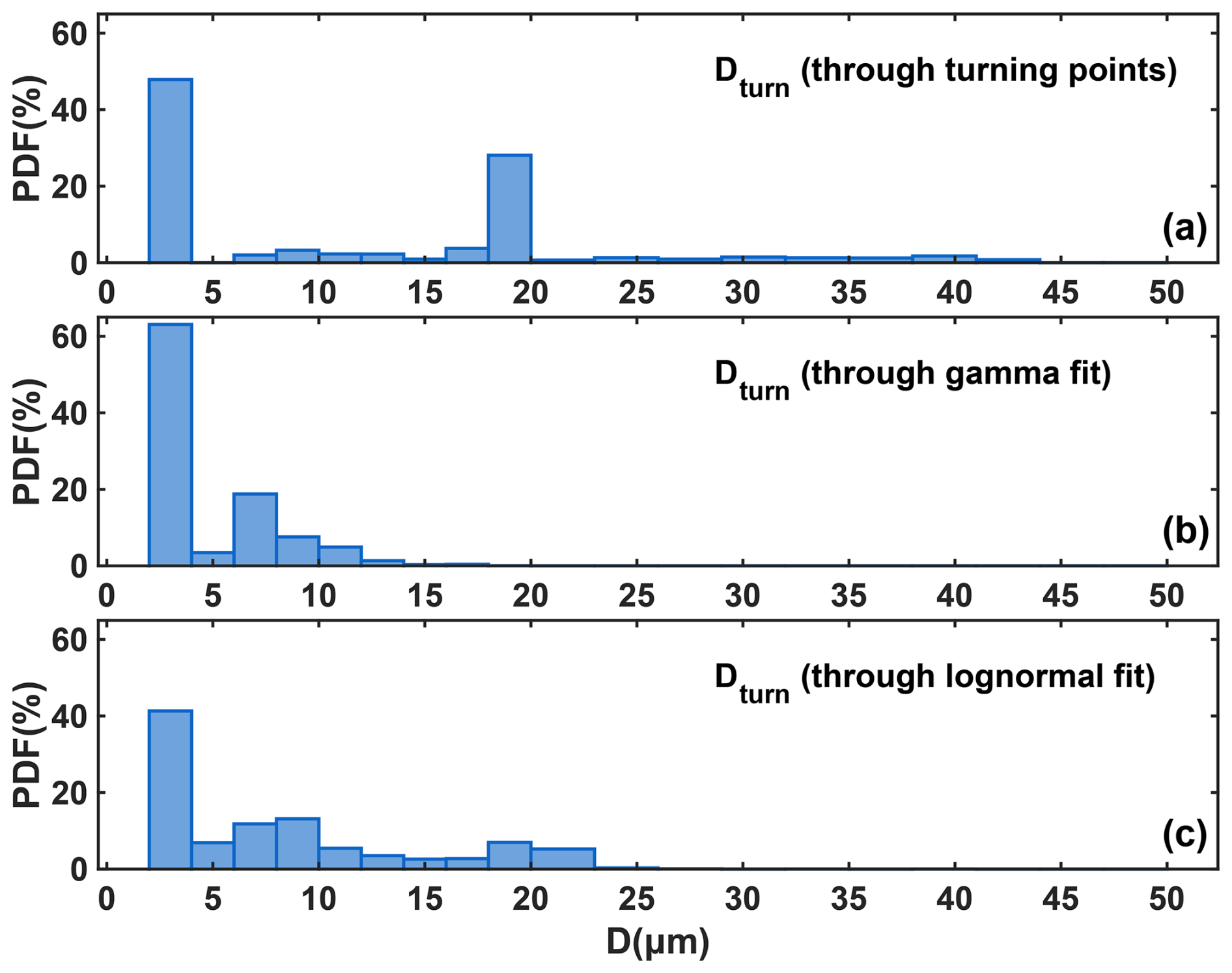
Figure 2 Distribution of D_turn derived from the turning-point method (a), gamma fitting (b), and lognormal fitting (c).

Given that temporal resolution may influence the identification of DSD mode numbers and D_turns, we derived these quantities using both 1 and 5 min averaged DSDs. The results from the lognormal distribution are presented here, while those from the gamma distribution are provided in the Fig. A11 in the Appendix. As the two resolutions produced only minor differences (Fig. 3), a 5 min averaging interval was used in this work to reduce the influence of noise.

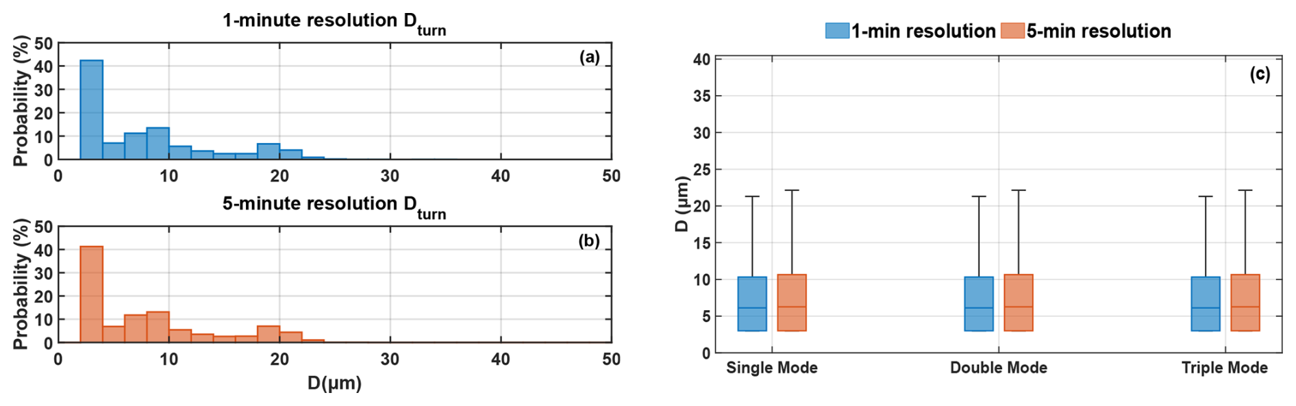
Figure 3 The D_turn distributions of all DSDs obtained using lognormal distribution at 1 min resolution (a), 5 min resolution (b), and the D_turn distributions by DSD type at both resolutions (c).

3 Results

3.1 Overview of fog microphysics

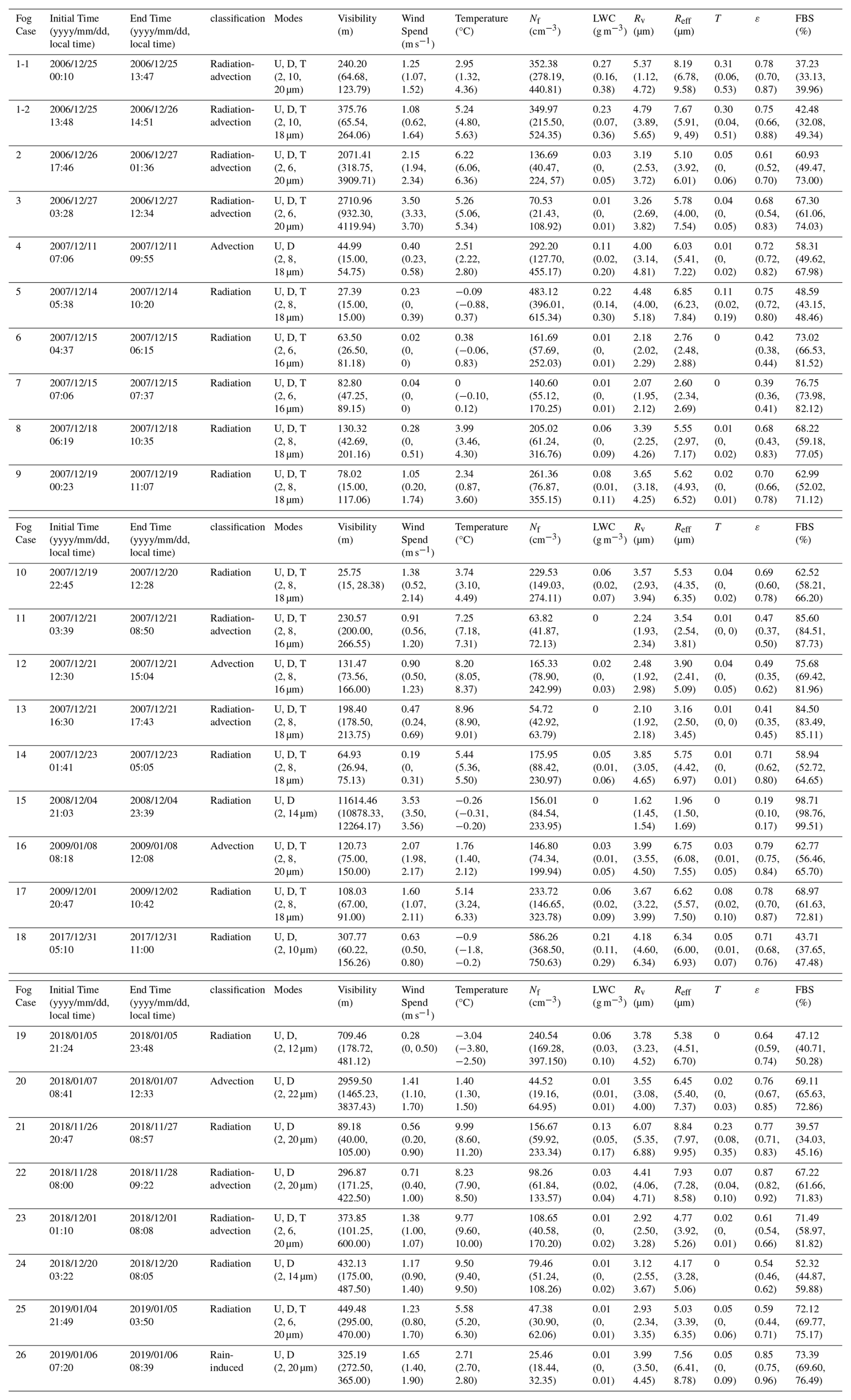
The fog type, meteorological variables (temperature, wind speed), visibility, and summary statistics of N_f, LWC, R_v, R_eff, ε, T and FBS for each event are provided in Table A1 of the Appendix. Among the 27 fog events, 14 were classified as radiation fog, 8 as radiation-advection fog, 4 as advection fog, while 1 event was likely associated with raindrop evaporation as it occurred after precipitation. Compared to other fog types, radiation-advection fog typically exhibits longer duration, slightly higher wind speed and temperature. The average N_f, LWC, R_v and R_eff vary over the ranges of 25–586 cm⁻³, 0–0.27 g m⁻³, 1.6–6 µm, 1.9–8.2 µm, respectively, which shows greater N_f, lower LWC and smaller droplet sizes comparing to semi-urban area in Paris, France (Mazoyer et al., 2022) and rainforest area in Xishuangbanna, China (Wang et al., 2021). In the meantime, significant variability in the microphysical properties is observed between different events. Among all DSDs, unimodal, bimodal, and trimodal distributions account for 5 %, 49 %, and 46 %, respectively. Unimodal DSDs exhibit the highest mean N_f, LWC and T, whereas bimodal DSDs have the largest R_v, R_eff and relative dispersion (ε), indicating larger droplet sizes and a broader size distribution. Trimodal DSDs show the highest FBS value.

Table 1 Microphysical characteristics of single mode, double mode and triple mode DSDs, the first row shows the mean values, in the parentheses are the 25th and 75th percentiles of each characteristic.

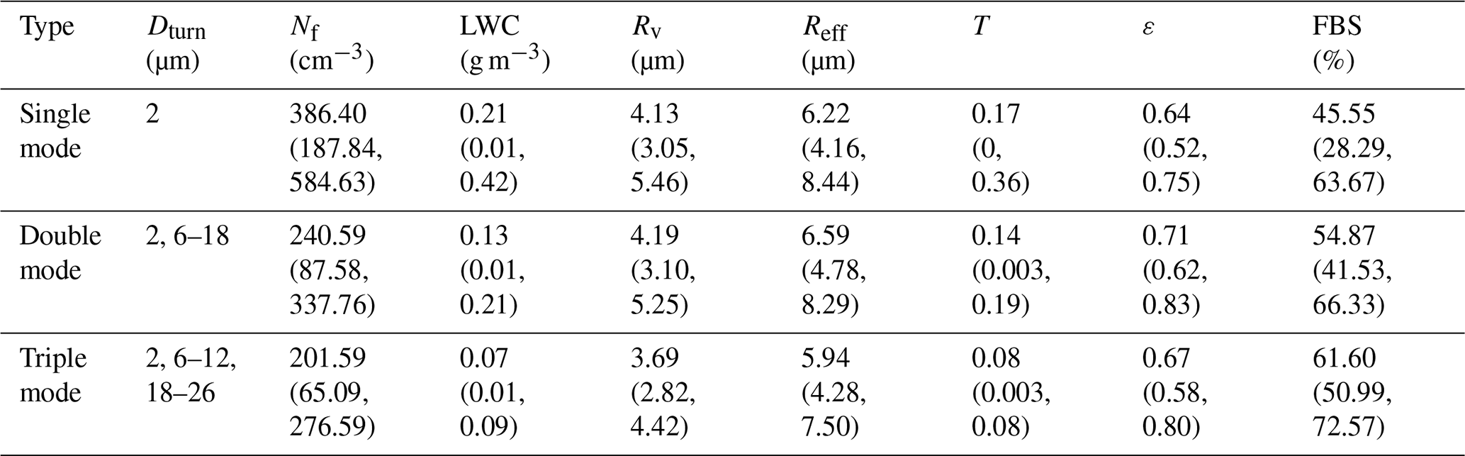
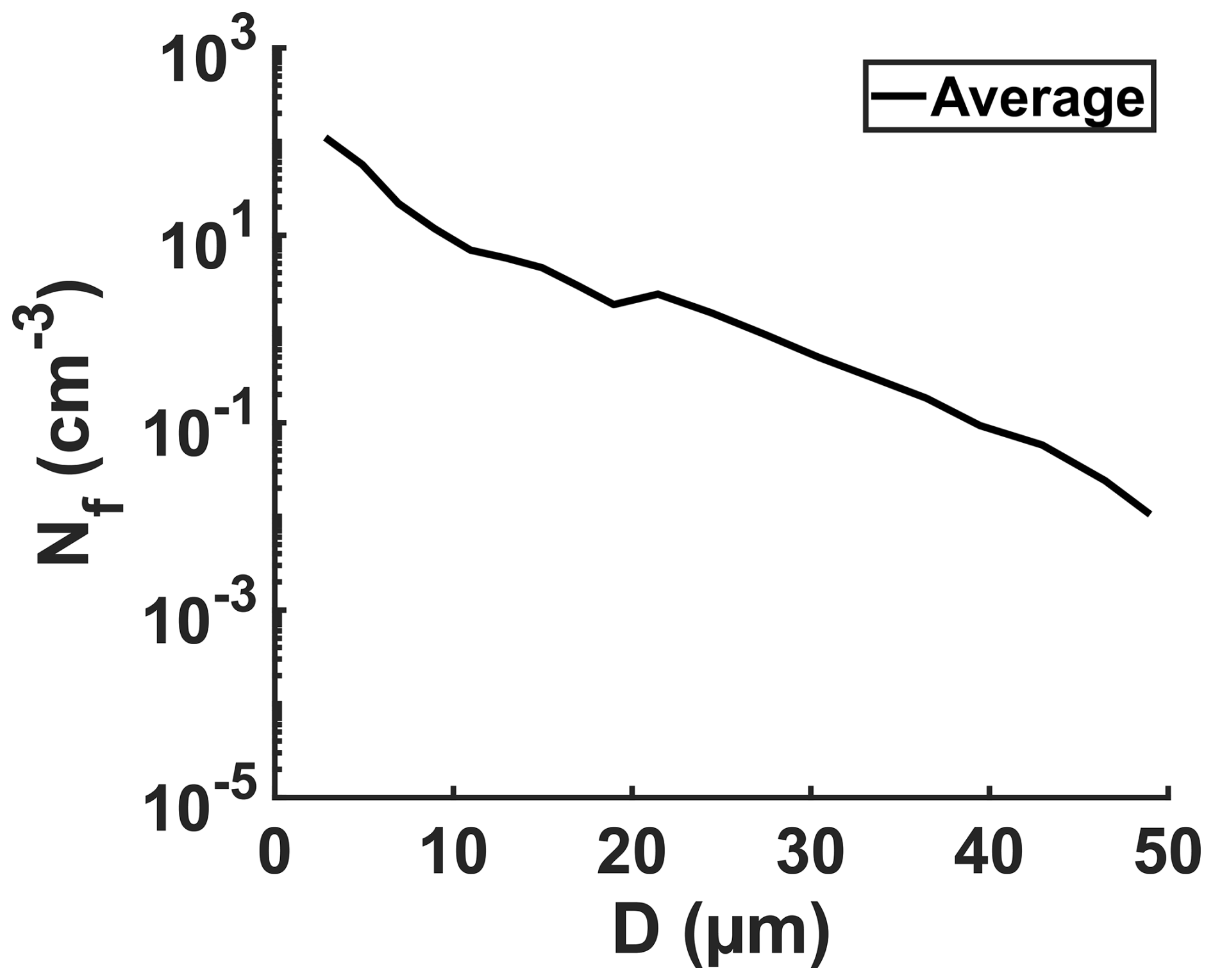
Figure 4 presents the mean DSDs for different mode types averaged over all fog cases (panel a) and over cases excluding Fog Case 1–2 (panel b). The mean DSD spectrums are sensitive to cases with high N_f and long durations, such as Fog Case 1–2 (F1–2). In particular, 50 % of the unimodal DSDs originate from F1–2, leading to higher N_f in the mean unimodal DSD spectrum than in other DSD types when all cases are included. For all cases, the mean spectrum of unimodal DSDs exhibits the highest N_f, particularly for droplets with diameters below 10 µm. In contrast, bimodal and trimodal DSDs show N_f at diameters below 10 µm that are very close to those of the mean spectrum of all DSDs. As aerosol activation is governed by environmental supersaturation and aerosol hygroscopic properties (Shen et al., 2018; Wang et al., 2019), the similar N_f at small diameters may indicate that aerosol activation persists throughout fog development, despite changes in the number of DSD modes. Within the diameter range of 10–50 µm, bimodal DSDs exhibit higher N_f than trimodal DSDs, consistent with their larger R_v, R_eff and ε.

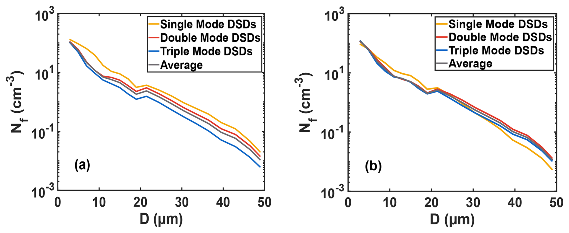
Figure 4 Average spectrums of fog DSDs for different mode types over all fog cases (a), and average spectra of fog DSDs with different modes excluding Fog Case 1–2 (b).

In the following section, five representative cases are selected to examine the lifecycle characteristics of fog events with different modes and the evolution of DSDs throughout the stages of fog formation, development, and dissipation.

3.2 Mode transitions and possible mechanisms

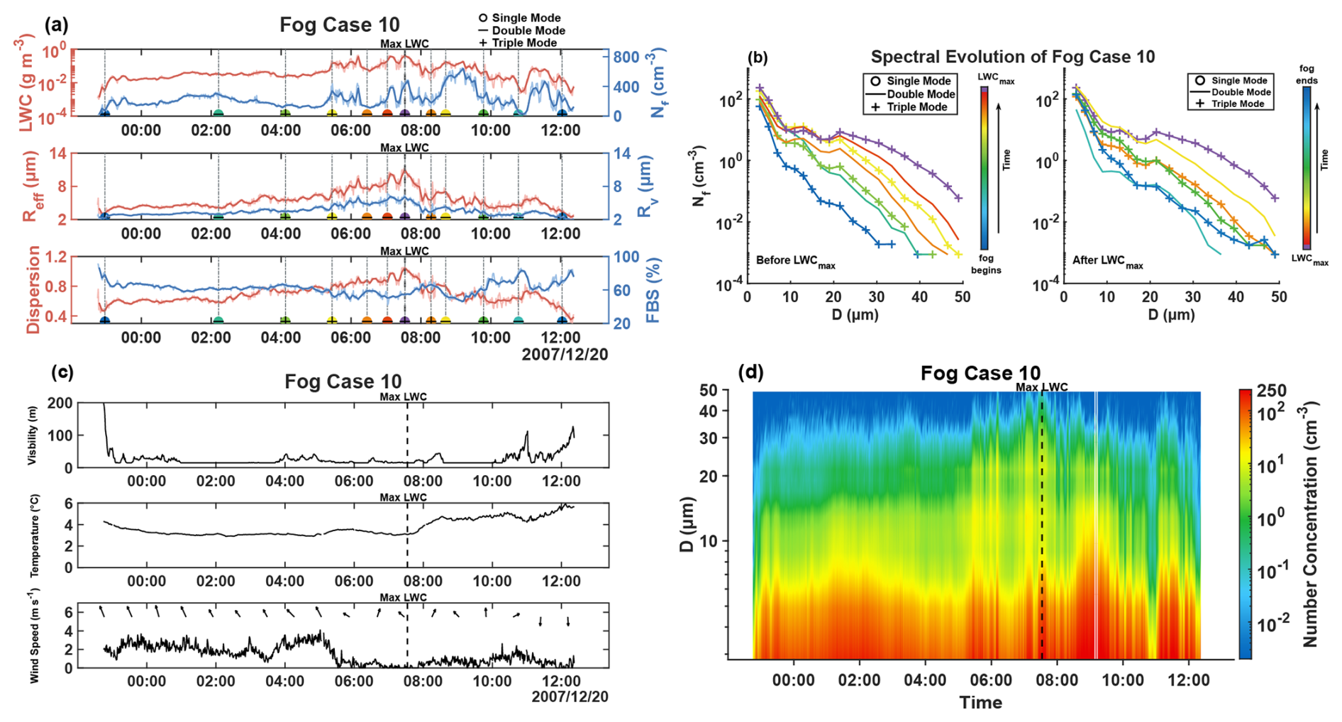
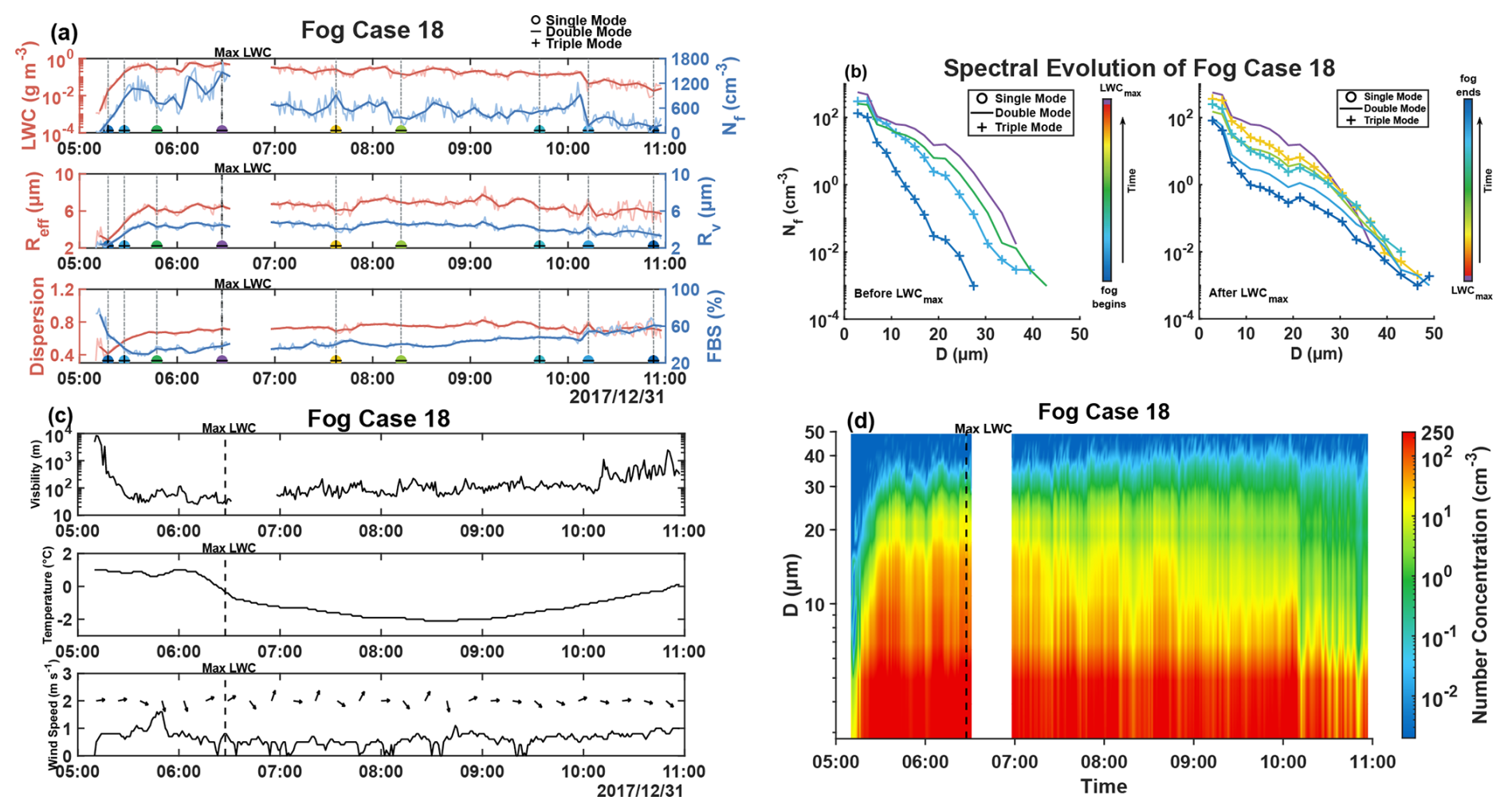
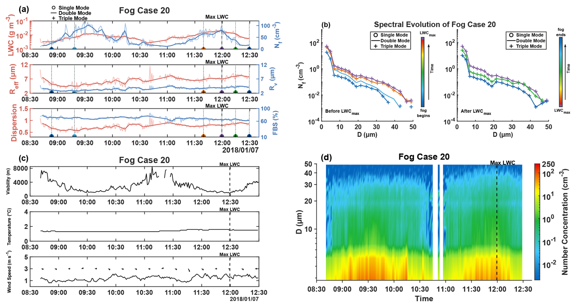
Figures 5–9 presents the temporal evolution of meteorological variables, visibility, microphysical properties, and droplet spectrum for the five selected cases. Surface, 850, and 700 hPa synoptic conditions preceding each fog event are provided in the Appendix (Figs. A13–A17). MODIS 3.9 µm shortwave infrared and visible channel imagery for Fog Case 1–1 (F1–1), Fog Case 10 (F10), and Fog Case 20 (F20) are provided in the Appendix (Figs. A8–A10). For Fog Case 4 (F4) and Fog Case 18 (F18), no satellite imagery is available within the fog period because the overpass times of the polar-orbiting satellite did not coincide with the observations. The 1 s temporal evolution of the DSDs are shown in Fig. A18. Among the five fog cases, F4 and F20 have relatively short durations and distinct formation-dissipation lifecycle. Both F1–1 and F18 experience rapid growth, whereas F10 exhibits pronounced temporal fluctuations during its lifecycle evolution. The maximum LWC used as an indicator of mature phase is marked in Figs. 5–9.

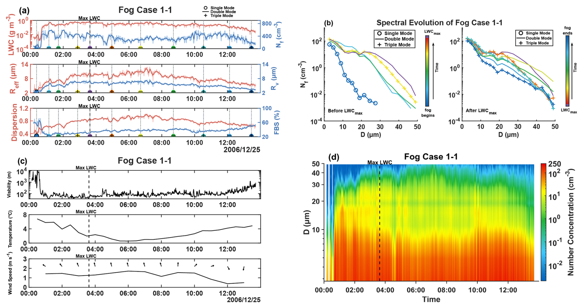
Figure 5 Panel (a) is the temporal evolution of N_f, LWC, R_v, R_eff, FBS and ε for fog case 1–1, the dark lines represent 5 min averaged values while the light lines are 1 min averaged values. Panel (b) is the 5 min average DSD. As the fog develops, the colors vary from blue to red, with the DSD at the time of maximum LWC marked in purple. From the time of maximum LWC to fog dissipation, the colors gradually shift from purple back to blue. Each DSD in (b) is marked in (a) using colors and symbols (circles, lines, and plus signs), where the colors denote time and the symbols indicate the modal type of the DSD. Panel (c) is the temporal evolution of visibility, temperature and wind speed, with wind direction represented by wind barbs. Panel (d) is the 1 min temporal evolution of DSDs.

Figure 6 Same as Fig. 5, but for fog case 4.

Figure 7 Same as Fig. 5, but for fog case 10.

Figure 8 Same as Fig. 5, but for fog case 18.

Figure 9 Same as Fig. 5, but for fog case 20.

Fog Case 1 (F1) was a radiation-advection fog event lasting 39 h. It formed under radiative cooling conditions, with sustained southwest warm and moist airflow supporting its long duration (Fig. A13). To enable a clearer and more detailed analysis of its microphysical characteristics, it was divided into two events at approximately the 14th hour after fog formation, based on the temporal evolution of N_f and LWC. The exact initial and end times of these two events, as well as their positions within the full fog lifecycle (F1), are provided in Table A1 and Fig. A12.

F1–1 experienced a rapid development after formation. During the first hour after fog formation, visibility decreased rapidly, and N_f increasing to approximately 600 cm⁻³. Following the drastic intensification there is a relatively stable phase lasting about 11 h, during which slowly decreasing temperature and steady wind direction created favorable conditions that maintain relatively high N_f and LWC. During fog formation and development, the DSD transitions among unimodal, bimodal, and trimodal. As the LWC approaches its maximum, N_f in the 5–20 µm range decreased, while those above 20 µm increased rapidly, suggesting a mass transfer from smaller to larger droplets as the DSD broadens toward larger droplets. During this stage, the DSD is predominantly bimodal. After 25 December 2006 10:00 LT, as N_f and LWC gradually decrease, the DSD again alternates between bimodal and trimodal (Fig. 5).

F4 is an advection fog event. Under the influence of a high-pressure ridge, the low-level atmosphere was stable with weak winds. Warm, moist air at 850 hPa was advected over a colder surface, cooled and condensed to form fog (Fig. A14). It shows a clear formation-dissipation evolution. About 40 min after fog formation, visibility gradually decreased as N_f and LWC increased. Temperature was relatively low during the formation and development stages, favoring fog persistence. Before LWC reaches its maximum, N_f and LWC continue to increase, followed by a gradual decrease after maximum LWC. R_v, R_eff and ε are positively correlated with LWC, while FBS shows a negative correlation. At the beginning of fog formation, transitions between bimodal and trimodal are more frequent. As the fog develops, the N_f of the DSD gradually increases, with a more pronounced enhancement in droplets within the 10–20 µm size range. During fog dissipation, transitions also occur with N_f gradually decreasing across all size ranges (Fig. 6).

F10 formed as a radiation fog under high-pressure control and weak surface winds (Fig. A15) and remained stable with relatively low N_f and LWC for the first 6 h. Under these stable conditions, the DSDs persisted in trimodal with little variation. After 20 December 2007 06:00, rising temperature and variable wind direction enhanced turbulent mixing and promoted fog development. N_f and LWC increased with pronounced fluctuations, corresponding changes were observed in the DSDs, as transitions between bimodal and trimodal distributions occurring frequently. Both R_v and R_eff increased with fluctuations, corresponding to the marked increase in N_f of droplets larger than 20 µm as shown by the DSD. During the dissipation stage, when N_f and LWC gradually decrease, trimodal DSDs are more prevalent with occasional transitions to bimodal (Fig. 7).

F18 is a radiation fog event formed under high-pressure conditions and near surface weak winds, driven by radiative cooling (Fig. A16). Blank areas in Fig. 8 indicate missing data. After fog formation, visibility decreases substantially, while N_f and LWC increase rapidly. Correspondingly, N_f across all size ranges rise quickly, and the DSD gradually transitions from a trimodal to a bimodal. After the LWC reaches its maximum, temperature decreases slowly and near-surface wind speeds remain weak, favouring fog maintenance. During this period and until gradual fog dissipation, the DSD alternates between bimodal and trimodal distributions.

F20 is an advection fog event. Under high-pressure control, easterly and southeasterly winds transported warm, moist marine air over a cold surface cooled by nocturnal radiative loss, providing favorable conditions for fog formation (Fig. A17). The stable temperature and wind direction as well as wind speeds below 3 m s⁻¹ favor fog maintenance. And the FBS remained consistently high at above 60 %. For F20, the DSDs were predominantly trimodal, without the pronounced increase in the N_f of droplets larger than 10 µm as observed in F18 and F10. Although this fog case exhibits two pronounced formation and dissipation cycles, transitions between bimodal and trimodal DSDs occur infrequently, likely due to its relatively low N_f and LWC.

Across the five fog cases analyzed above, transitions of the DSD among different modal types occur in all cases and are closely linked to the characteristics of the fog life cycle. In cases with relatively low N_f and LWC or weak temporal variability, such as F4 and F20, these transitions occur less frequently. In F10, frequent changes in DSD modal types coincide with pronounced oscillations in N_f and LWC. Both F1–1 and F18 exhibit explosive increases in N_f and LWC during fog formation, and as LWC approaches its maximum, bimodal DSDs occur more frequently. However, LWC in F1–1 is slightly higher than in F18, while the mean N_f in F18 is approximately 1.5 times that in F1–1. The resulting stronger competition for water vapor may suppress the formation of droplets larger than 20 µm, preventing the sustained occurrence of a bimodal DSD.

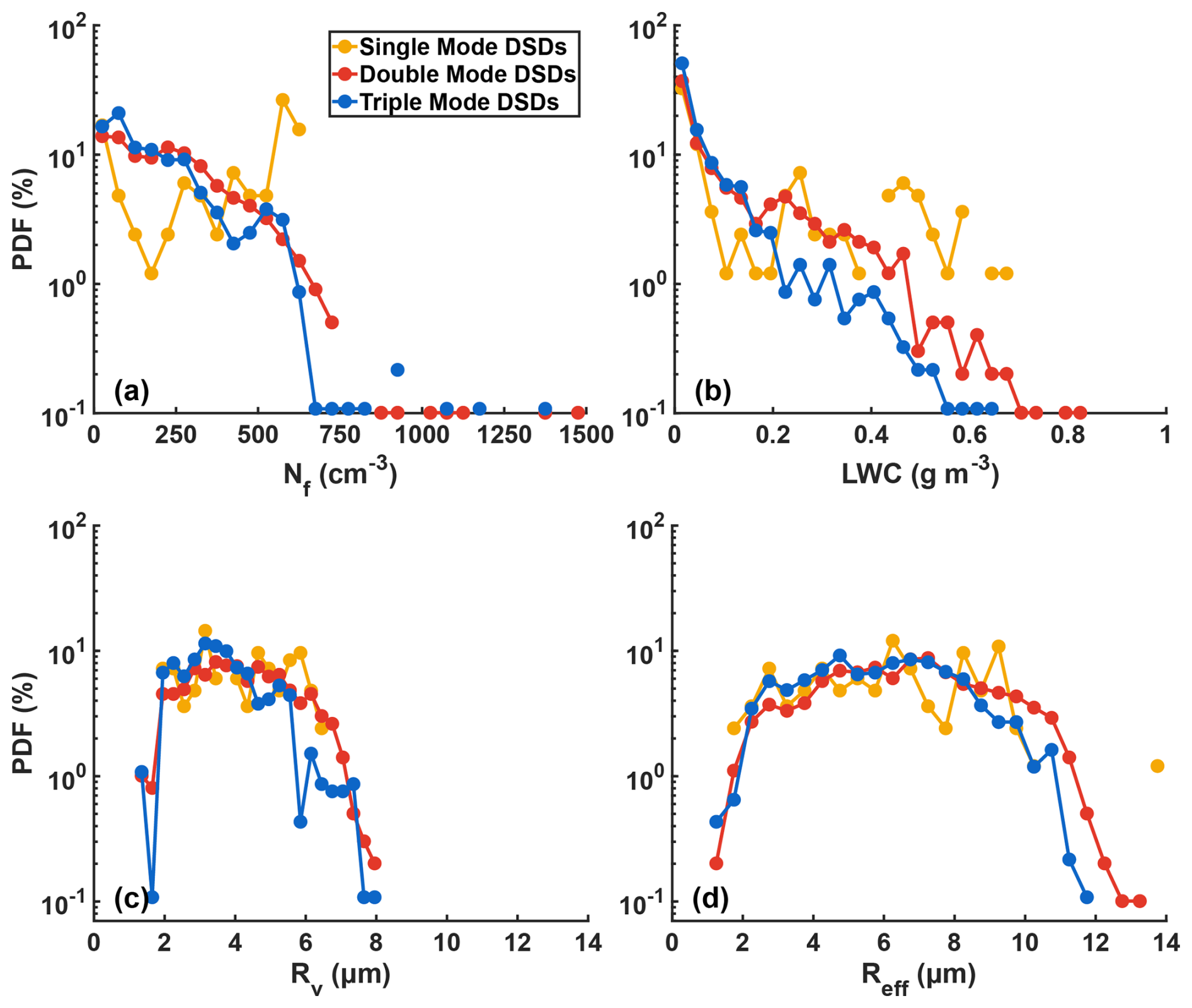
Figure 10 PDF distributions of N_f (a), LWC (b), R_v (c) and R_eff (d) for DSDs with different modes.

Figure 11 Average contributions of each DSD bin to N_f (a) and LWC (b) with different modes.

3.3 Correlation of modes and microphysical properties

Figure 10 presents the probability distributions of N_f, LWC, R_v and R_eff across unimodal and multimodal DSDs. The N_f distribution of unimodal DSDs differs markedly from those of bimodal and trimodal DSDs, with its probability density function (PDF) distributions mainly concentrated below 200 and above 400 cm⁻³. In particular, the PDF distributions above 400 cm⁻³ is higher than that of bimodal and trimodal DSDs. For bimodal and trimodal DSDs, the PDF of N_f decreases with increasing N_f, although bimodal DSDs show slightly higher PDF values than trimodal DSDs in the range of 250–500 cm⁻³. The LWC distribution of unimodal DSDs shows characteristics similar to its N_f distribution, with the highest PDF occurring at values exceeding 0.4 g m⁻³. Bimodal and trimodal DSDs exhibit similar distribution when LWC is below 0.2 g m⁻³, whereas bimodal DSDs have higher PDF values and a broader distribution at LWC higher than 0.2 g m⁻³. For the R_v distribution, unimodal DSDs exhibit the narrowest range, mainly concentrated between 2 and 6 µm. Bimodal and trimodal DSDs have comparable ranges. However, trimodal DSDs are primarily concentrated between 2 and 4 µm, with the PDF decreasing rapidly beyond 4 µm, whereas bimodal DSDs show a more uniform distribution over the range of 2–7 µm. In terms of R_eff, unimodal DSDs exhibit the highest PDF values in the 8–10 µm range. Bimodal DSDs show the widest R_eff distribution, with PDF values above 8 µm exceeding those of trimodal DSDs. Trimodal DSDs are mainly distributed between 2 and 10 µm, with slightly higher PDF values than bimodal DSDs in the 2–5 µm range.

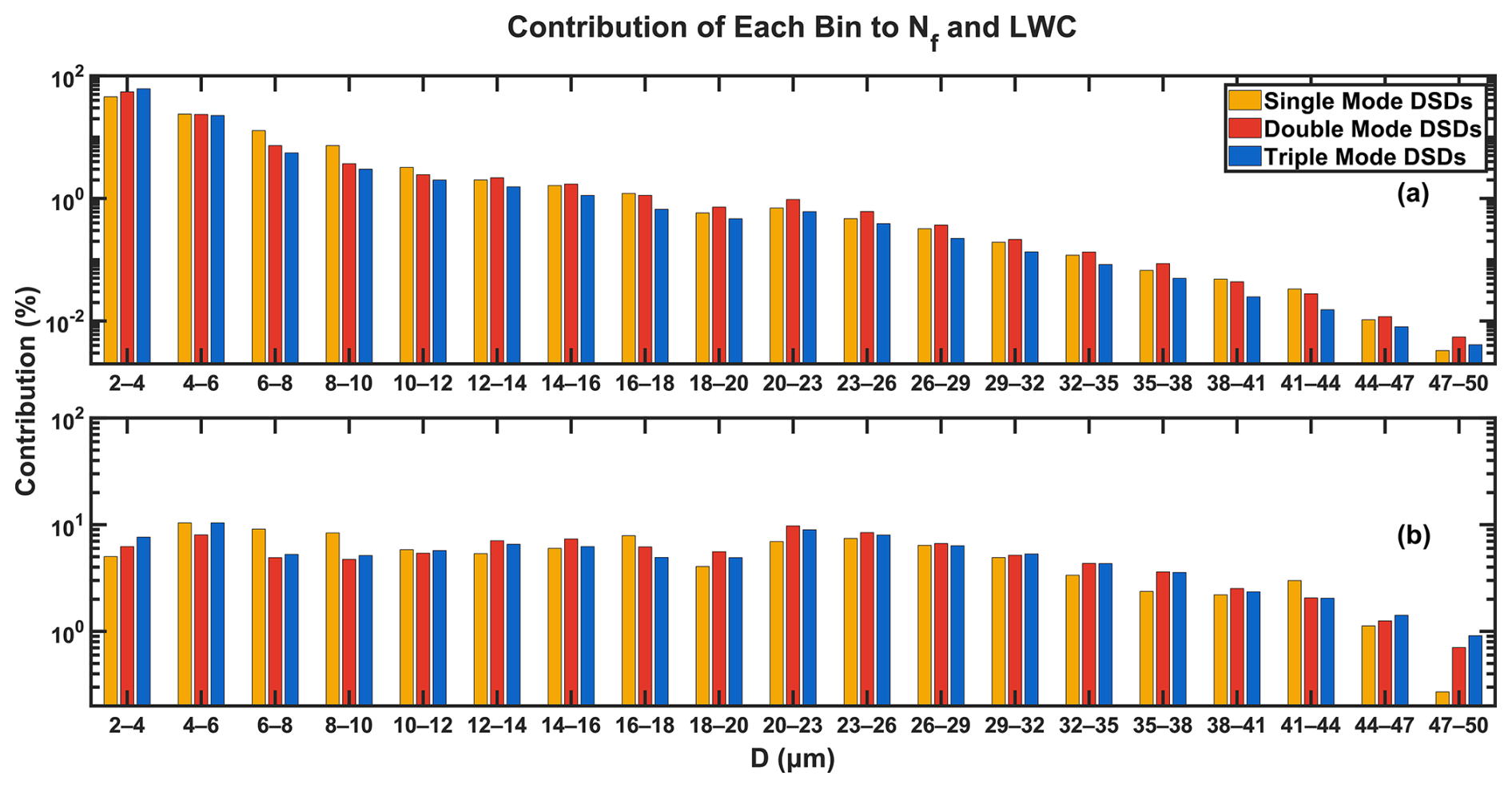
Figure 11 shows the average contributions of each droplet size bin to total N_f and LWC with different modes. The mean contribution of each size bin to the total N_f shows good consistency with the DSD modal distribution. For unimodal DSDs, the contribution of individual bins to N_f decreases with increasing droplet size. In contrast, bimodal DSDs exhibit an enhanced contribution to N_f in the 18–29 µm size range. Compared with trimodal DSDs, droplets larger than 10 µm contribute more to the N_f of bimodal DSDs. For LWC, in unimodal DSDs droplets in the 2–10, 16–18, and 20–29 µm diameter ranges all make noticeable contributions. In bimodal and trimodal DSDs, droplets at other sizes contribute relatively less to LWC compared with those in the 2–6 and 20–29 µm diameter ranges. However, compare to trimodal DSDs, droplets in the 12–20 µm range contribute slightly more to LWC in bimodal DSDs.

3.4 Performances and improvement of gamma and lognormal fitting

Bulk microphysical schemes commonly represent DSDs with gamma or lognormal distributions, making the accuracy of these representations critical to performance of numerical simulation. To evaluate the validity of the gamma and lognormal distribution for winter fog in Nanjing, mean DSDs of 27 observed fog events are fitted using the form of Eqs. (12) and (13) with i=1. For the fog events examined in this study, both gamma and lognormal distribution provide a good fit to the average DSD in the small-droplet range (2–10 µm), but significantly underestimates number concentrations as droplet size increases, especially the gamma distribution. In multimodal DSDs of the examined events, additional modes appear besides the mode near 2 µm, which likely contribute to the poor fit. The probability distribution of D_turn obtained from lognormal fitting across all DSDs (Fig. 2c) indicates that the other two modes occur primarily around 10 and 20 µm. Therefore, segmented gamma and lognormal fitting was conducted using 10 and 20 µm as partition points (Fig. 12b, c, d, f, g, h). When DSDs are segmented at 10 µm, the fit increasingly underestimates number concentrations for diameters above 20 µm. Segmentation at 20 µm produces good agreement in the 2–10 and 20–50 µm ranges, although substantial deviations remain in the intermediate 10–20 µm range. Based on these results, a three-segment gamma fitting approach was applied using 10 and 20 µm as partition points (Fig. 12d, h). This approach significantly improves the overall fit ranging from 2 to 50 µm, providing a more accurate representation of the whole DSDs.

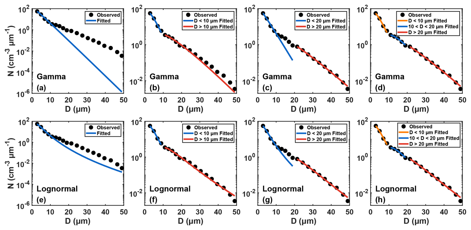
Figure 12 Gamma and lognormal fitting of the mean spectrum: original fit (a, e), two-segment fitting with a breakpoint at 10 µm (b, f), two-segment fitting with a breakpoint at 20 µm (c, g), and three-segment fitting with breakpoints at 10 and 20 µm (d, h).

To demonstrate that the superior performance of the three-segment gamma and lognormal fitting is due to the physically meaningful segmentation based on the characteristics of DSDs, rather than merely the increased number of segments, we evaluated the performance of alternative segmented fitting. Since the gamma and lognormal distributions are nonlinear, two fitting points would fall on a straight line and cannot constrain the distribution, potentially leading to non-identifiable or ill-posed parameter estimates. Therefore, the segmentation points must satisfy two conditions: (a) the full spectrum must be divided into three segments, and (b) each segment must contain at least three bins. Under these constraints, 66 feasible segmentation combinations exist. Using each set of segmentation points, we performed gamma and lognormal fits for all DSDs and retrieved the corresponding N_f, LWC, R_v and R_eff. The absolute deviations between the retrieved values and the observed ones were compared for both the alternative fittings and the fixed 10 and 20 µm segmentation (Fig. 13). For all four microphysical parameters, the deviations from the fixed-segmentation fitting are significantly smaller than those from alternative segmentation. A two-sided binomial test was conducted to evaluate the probability that the fixed segmentation outperforms the alternative segmentation. For both distributions, the 95 % confidence interval is [0.986, 1.000] with a p-value of $\mathrm{2.23}\times {\mathrm{10}}^{-\mathrm{308}}$. These p-values are far below the 0.05 significance threshold. These results confirm the effectiveness of the 10 and 20 µm segmentation for both gamma and lognormal distribution.

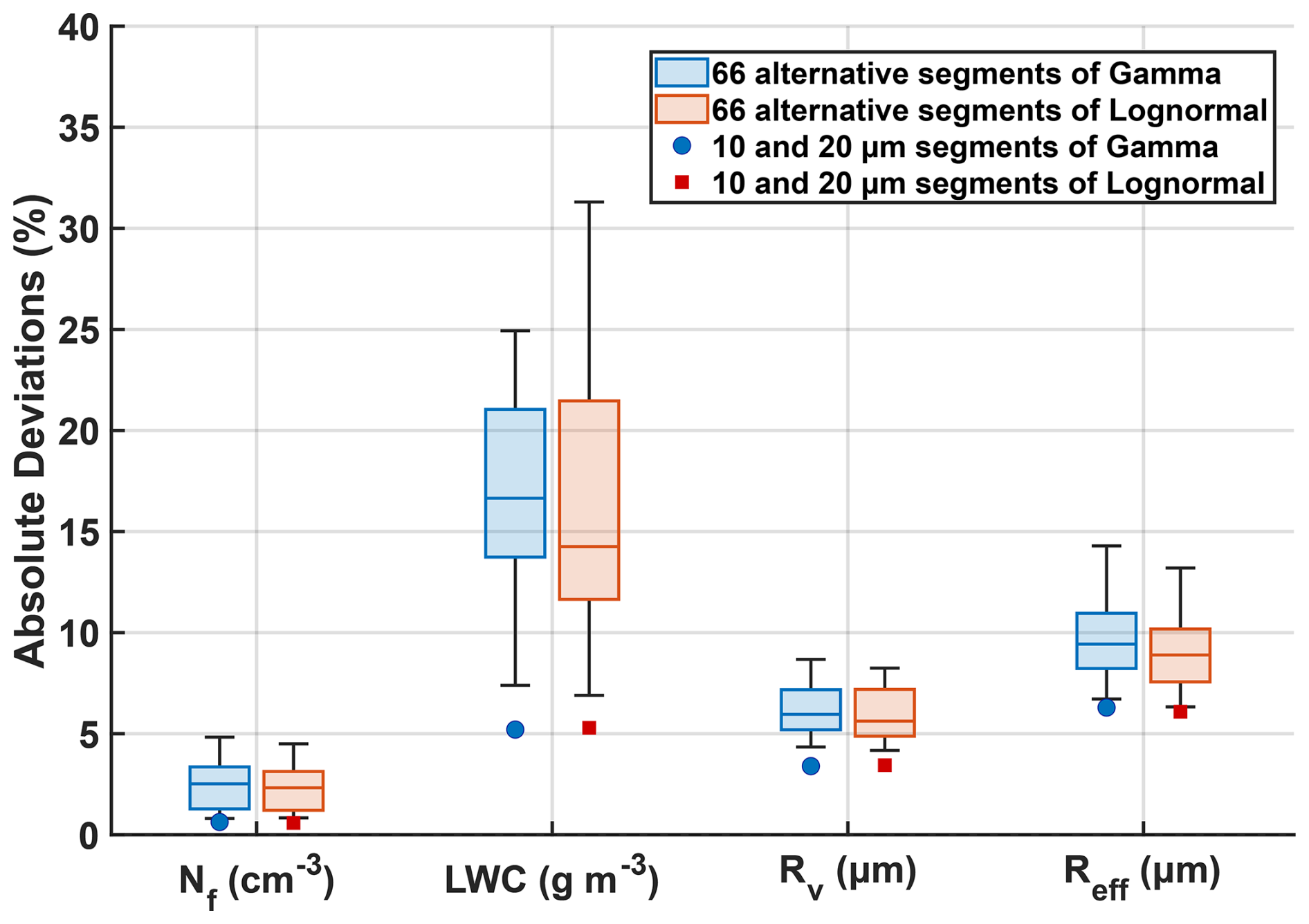
Figure 13 Boxplots of the mean absolute deviations from 66 alternative segmented fittings, with red and blue dots indicating the mean deviations from the fixed 10 and 20 µm segmentation.

To further evaluate the performance of the gamma and lognormal fitting with different breaking points, N_f, LWC, R_v and R_eff were calculated based on both the original and segmented fit. These results were then compared with those derived from observations. The deviation distribution between fitted and observed results are analysed in Fig. 14, and the correlation between them are showed in Fig. A19. The non-segmented gamma fit significantly underestimates the N_f of droplets larger than 10 µm, leading to underestimation of all derived microphysical quantities. The N_f calculated from the two-segment fit with a breakpoint at 10 µm is close to observation, but the derived LWC are still underestimated. For the fit segmented at 20 µm all microphysical quantities are underestimated, likely due to underrepresentation of droplet concentrations in the 10–20 µm range. Compared to the non-segmented gamma fit approach, the three-segment fitting shows substantial improvement in the high N_f regime (N_f > 700 cm⁻³) and in LWC estimation as the results are tightly clustered around the zero-deviation line and the 1 : 1 line (Fig. A19). Also, the fitting accuracy for R_eff and R_v is also improved for both gamma and lognormal fitting.

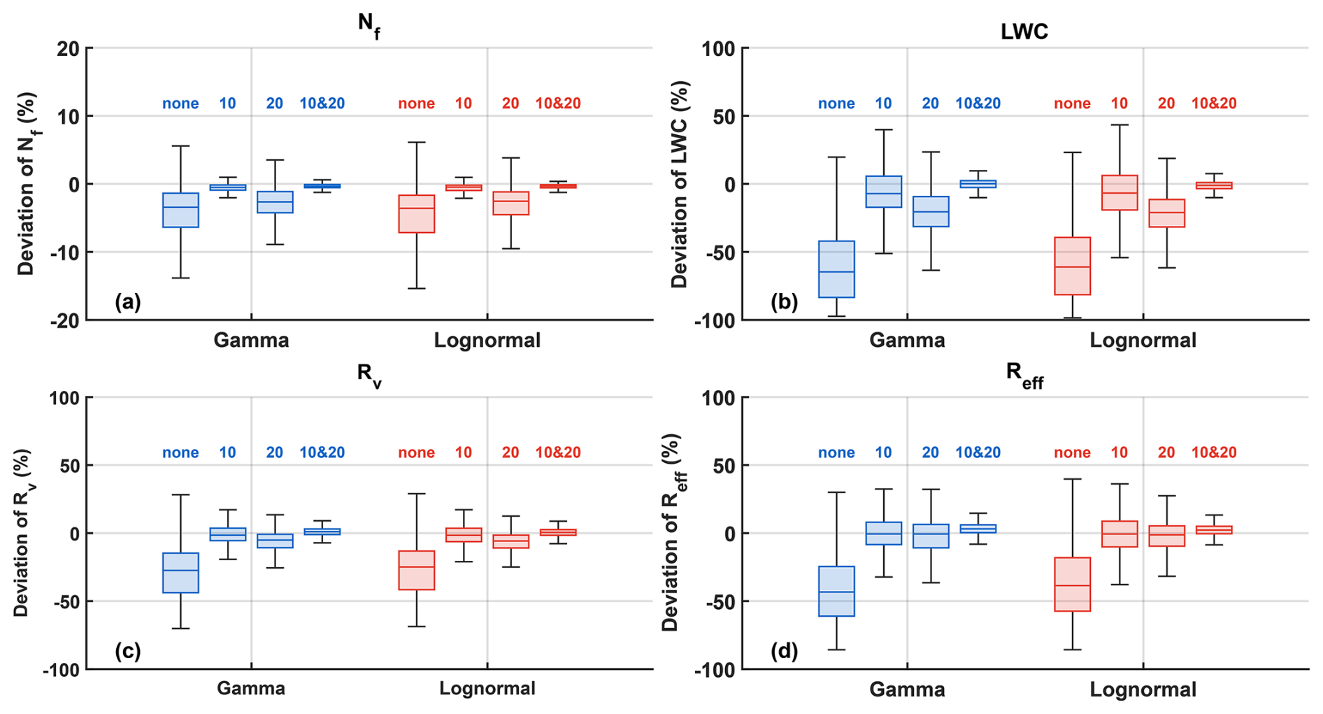
Figure 14 Deviation distribution of N_f, LWC, R_v and R_eff between observation spectrum and the gamma and lognormal fitted spectrum. The number above each boxplot indicates the segmentation position (µm); “none” denotes no segmentation point applied.

Except for the non-segmented gamma fitting, the other three segmented approaches exhibit a clear pattern in estimating R_eff: underestimation primarily occurs when the observed R_eff < 6 µm, while overestimation tends to occur when the observed R_eff > 6 µm (Fig. A19). This pattern is particularly pronounced in the fitting segmented at 20 µm, whereas the three-segment fitting shows notable improvement in reducing underestimation at lower R_eff values.

Cloud optical thickness (τ) and single-scattering albedo (ω₀) are key parameters for evaluating the Twomey effect (Stephens, 1984; Twomey and Bohren, 1980). τ can be calculated with

$$\begin{array}{}\text{(16)}& \mathit{\tau }=\int {\displaystyle \frac{\mathrm{3}\mathrm{LWC}}{D_{\mathrm{eff}}}}\mathrm{d}z\end{array}$$

where z is the thickness of the cloud or fog layer (Stephens, 1978). When assuming cloud or fog is vertically homogeneous, Eq. (16) can be simplified as

$$\begin{array}{}\text{(17)}& {\displaystyle \frac{\mathit{\tau }}{\mathrm{d}z}}={\displaystyle \frac{\mathrm{3}\mathrm{LWC}}{D_{\mathrm{eff}}}}\end{array}$$

where $\frac{\mathit{\tau }}{\mathrm{d}z}$ represents the average optical thickness per layer. The single-scattering albedo (ω₀) can be expressed by

$$\begin{array}{}\text{(18)}& \mathrm{1}-{\mathit{\omega }}_{\mathrm{0}}=\mathrm{1.7}{k}_{\mathrm{w}}{R}_{\mathrm{eff}}\end{array}$$

where k_w is the complex part of the refractive index of water. Equation (18) indicates the critical role of R_eff in the Twomey effect (Wang et al., 2019).

To more precisely assess the potential climate impact of inaccuracy in R_eff estimates from gamma and lognormal fitting, Eqs. (17) and (18) were used to calculate absorption coefficient and optical thickness based on both observed and fitted R_eff. This allowed evaluation of the extent to which gamma and lognormal fitting overestimates or underestimates these parameters. Results are showed in Fig. 15.

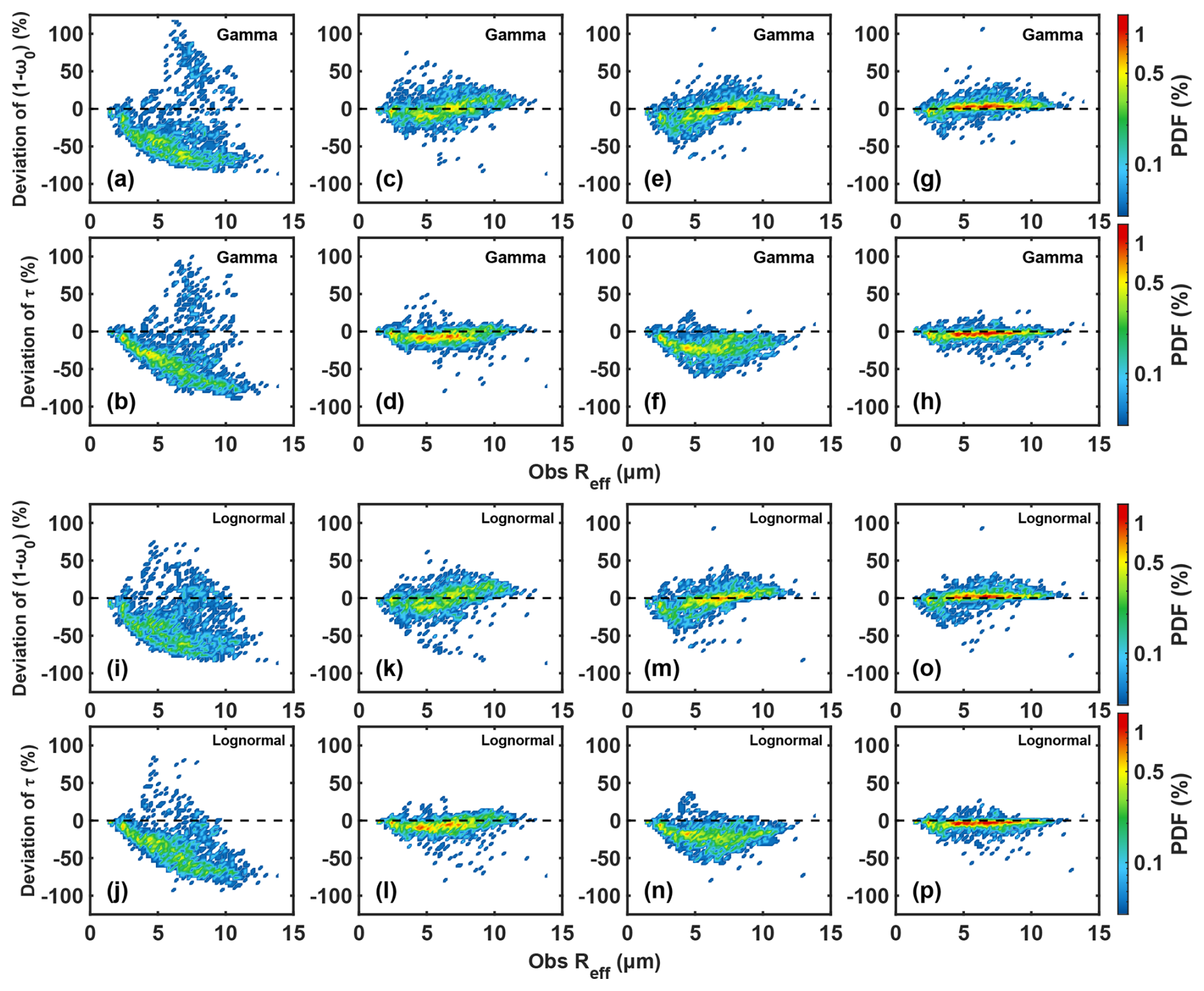
Figure 15 Correlation between absorption coefficient (1−ω₀) and optical thickness (τ) derived from observed spectrum and those computed from the gamma and lognormal fitted spectrum with no breakpoint (a, b, i, j), breakpoint at 10 µm (c, d, k, l), breakpoint at 20 µm (e, f, m, n) and breakpoint at 10 and 20 µm (g, h, o, p).

Due to its significant underestimation of the N_f of droplets larger than 10 µm, the non-segmented gamma and lognormal fitting notably underestimate absorption coefficient (1−ω₀) and optical thickness (τ) by up to 90 %. Compared to the fitting segmented at 20 µm, the fitting segmented at 10 µm more accurately captures absorption coefficient and optical thickness, yet still exhibits up to 50 % overestimation or underestimation of absorption coefficient. It is noteworthy that the 20 µm-segmented fitting generally underestimates optical thickness, likely due to the underestimation of the N_f for droplets in the 10–20 µm range.

In contrast, the three-segment fitting significantly improves the estimation of both absorption coefficient and optical thickness, with most deviations confined within ±20 %. The most notable improvements lie in reducing the underestimation of absorption coefficient and the overestimation of optical thickness, as the percentages of both underestimation and overestimation become very small.

Figure 16 Correlation between the N₀, μ and λ derived from the three-segment gamma fitting.

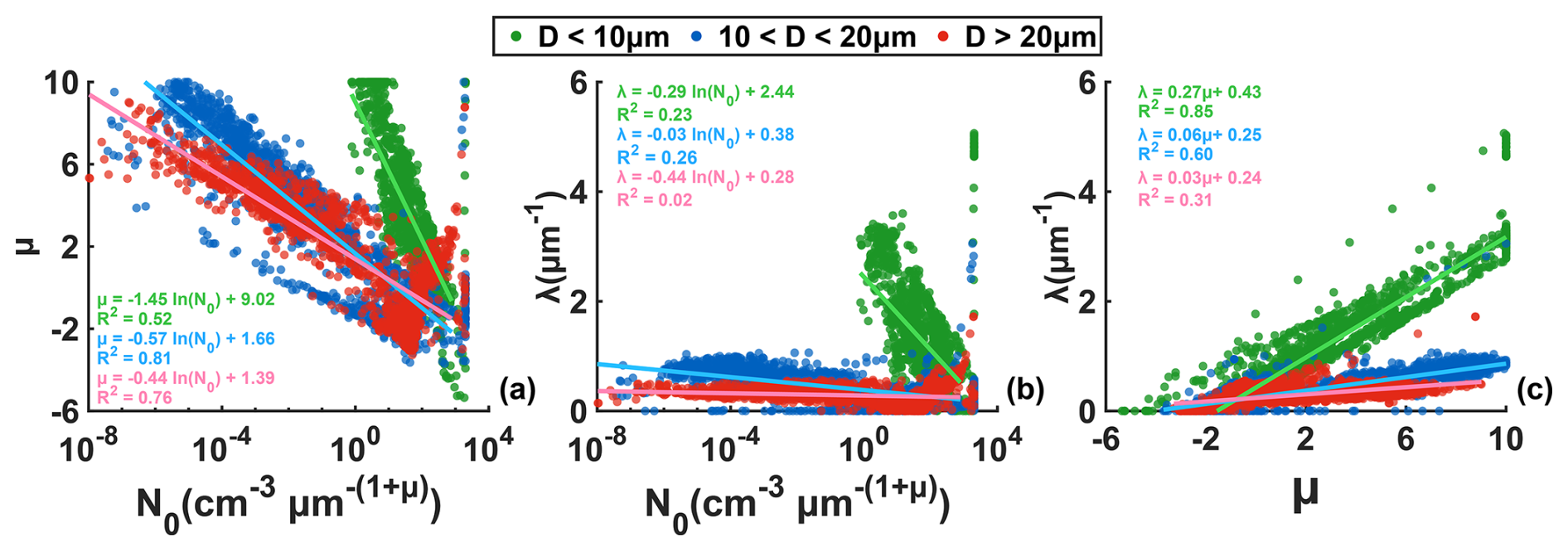
The interrelationships among the three fitting parameters obtained from the three-segment gamma fitting are shown in Fig. 16. For each segment, N₀ exhibits a negative correlation with both μ and λ, while μ and λ are positively correlated. In the D<10 µm segment, larger N₀ and λ are observed, indicating a narrower and more concentrated spectrum with a steep decline in number concentration as droplet size increases. For D>10 µm, N₀ shows a wider distribution with smaller λ, reflecting broader spectrum and higher number concentrations of larger droplets. Compared to the D>10 µm segments, N₀ in the D<10 µm range is more tightly gathered in a range of 10⁰–10³ cm⁻³ µm${}^{-(\mathrm{1}+\mathit{\mu })}$, suggesting that small droplet concentrations are higher and more consistent across different DSDs. Because the fitting parameters of lognormal distribution do not exhibit clear correlations, they are not shown here.

4 Conclusions

As a key parameter of fog microphysical processes, the droplet size distribution (DSD) is influenced by multiple macro- and micro-scale factors, exhibits significant temporal and spatial variability, and evolves throughout the fog lifecycle, thereby posing challenges for accurate fog prediction (Niu et al., 2012; Nelli et al., 2024). To gain a better understanding of how the DSD evolves over the fog lifecycle, this study investigates the microphysical characteristics of 27 winter fog events in Nanjing under polluted conditions, with a focus on the evolution of droplet size distributions (DSDs) throughout the fog lifecycle. Among the 27 fog cases, DSDs with single mode (2 µm), double mode (2, 6–18 µm) and triple mode (2, 6–12, 18–26 µm) were observed. The average N_f, LWC, R_v and R_eff vary over the ranges of 25–586 cm⁻³, 0–0.27 g m⁻³, 1.6–6 µm, 1.9–8.2 µm, which shows greater N_f, lower LWC and smaller droplets comparing to other clean regions such as the tropical rainforests of southwestern China (Wang et al., 2021). The main findings are as follows:

Among all fog cases, radiation fog accounts for the largest proportion and radiation-advection fog tends to persist longer. Variations in the number of DSD modes are closely linked to fog lifecycle characteristics and to changes in physical variables such as N_f and LWC. For fog events with relatively low N_f and LWC or relatively less intense formation and dissipation processes, transitions in DSD modal type are infrequent and occur mainly during the formation and dissipation stages. When N_f and LWC increase sharply, the DSD shows frequent modal transitions with an increasing prevalence of bimodal DSD. Moreover, when N_f and LWC exhibit strong oscillations, transitions among different modal types occur simultaneously and at high frequency.

Comparison of the retrieved physical parameters from segmented gamma and lognormal fitting with observations indicates that the three-segment fitting yields the best performance, especially in improving N_f and LWC estimation. Meanwhile, the three-segment fitting reduces the estimation deviations in R_eff, absorption coefficient and optical thickness from up to 90 % in the non-segmented fitting to below 20 %, demonstrating its effectiveness in improving fog DSD representation and microphysical characteristic retrieval.

These findings advance our understanding of fog droplet size distribution (DSD) evolution during fog lifecycles and the correlations between DSD modes and microphysical properties in polluted urban regions. The improved segmented gamma and lognormal fitting offer a new perspective for DSD parameterization and demonstrates strong potential for improving the representation of cloud/fog microphysical processes in weather prediction and climate models. It should be noted that this study is primarily based on observational data and focuses on analyzing the microphysical characteristics and their evolutions. The underlying physical processes and mechanisms governing fog evolution as well as the interactions and relative importance of different controlling factors, remain to be clarified through enhanced analyses of aerosol background conditions and sensitivity experiments on relevant physical processes using numerical simulations. In addition, only a three-parameter gamma and lognormal distribution was used to fit and refine the mean DSD. The comparative performance of alternative distribution and evaluate the influence of different parameterizations on fitting accuracy could be explored in future studies.

Appendix A

A1 Details on the upper and lower bounds of parameters used for gamma and lognormal fitting

In this study, DSDs were fitted using gamma and lognormal distributions to determine the number of modes and their corresponding D_turn, which are also shown below.

For gamma distribution:

$$\begin{array}{}\text{(A1)}& n\left(D\right)=\sum _{i=\mathrm{1}}^{\mathrm{3}}{n}_i\left(D\right)=\sum _{i=\mathrm{1}}^{\mathrm{3}}{N}_{\mathrm{0},i}{D}^{{\mathit{\mu }}_i}{e}^{-{\mathit{\lambda }}_{i}D}\end{array}$$

For the lognormal distribution:

$$\begin{array}{}\text{(A2)}& \begin{array}{rl}n\left(D\right)& =\sum _{i=\mathrm{1}}^{\mathrm{3}}{n}_i\left(D\right)\\ & =\sum _{i=\mathrm{1}}^{\mathrm{3}}{\displaystyle \frac{N_{\mathrm{0},i}}{\mathrm{2}{\mathit{\pi }}^{\mathrm{1}/\mathrm{2}}{D}_i\ln {\mathit{\sigma }}_{\mathrm{g},i}}}\exp \left(-{\displaystyle \frac{(\ln D_i-\ln D_{\mathrm{g},i}{)}^{\mathrm{2}}}{\mathrm{2}(\ln {\mathit{\sigma }}_{\mathrm{g},i}{)}^{\mathrm{2}}}}\right)\end{array}\end{array}$$

Fits with different numbers of modes were performed, and the optimal solution was obtained for each distribution.

For the gamma distribution, no predefined size ranges were prescribed. Unimodal, bimodal, and trimodal gamma distributions were fitted separately, allowing the fitting procedure to automatically identify the optimal solution.

In the lognormal distribution, three possible modes (approximately 2, 10–18, and 18–23 µm) were identified based on the mean DSD of all cases (Fig. A1). To minimize subjective influence, relatively broad bounds of D_g were assigned to the parameters under different values of i. For unimodal distributions (i=1), D_g were constrained to the range 2–50 µm. In bimodal distributions (i=2), two candidate mode diameter combinations were considered: (2, 11 µm) and (2, 21 µm). Accordingly, different lower and upper bounds were specified for D_g. For the 2 and 11 µm combination, the bounds were set to 2–10 and 5–20 µm; for the 2 and 21 µm combination, the bounds were 2–10 and 15–50 µm. In trimodal distributions (i=3), the bounds for D_g were set to 2–50, 5–20, 15–50 µm. The discrete representation of the lognormal distribution parameter σ_g is given by

$$\begin{array}{}\text{(A3)}& \ln {\mathit{\sigma }}_{\mathrm{g}}={\left({\displaystyle \frac{\sum n_i(\ln D_i-\ln D_g{)}^{\mathrm{2}}}{\sum n_i-\mathrm{1}}}\right)}^{\mathrm{1}/\mathrm{2}}\end{array}$$

in which $\ln D_{\mathrm{g}}=\frac{\sum n_i\ln D_i}{\sum n_i}$. In this study, the maximum calculated value of σ_g is approximately 2.34. Therefore, the range of σ_g was set to 0–2.5. In the meantime, N₀ was set to 0–2000 cm⁻³.

Figure A1 Average spectrums of all fog DSDs.

A2 Model selection criteria for unimodal, bimodal, and trimodal fits and representative examples

In this study, based on comparisons with the turning-point method and the gamma fitting results, the lognormal distribution was selected to determine the number of DSD modes and the corresponding D_turn. Because two sets of fitting parameters were specified for the bimodal distribution, two fitting results were obtained, resulting in four candidate fits for each DSD in total. Intersections between adjacent fitted components were required, and the D_turn derived from these fits were not allowed to occur in the same or adjacent bins. Among the fits that satisfy this criterion, the one with the lowest AIC and BIC was selected to determine the number of modes and the mode diameters of the DSD.

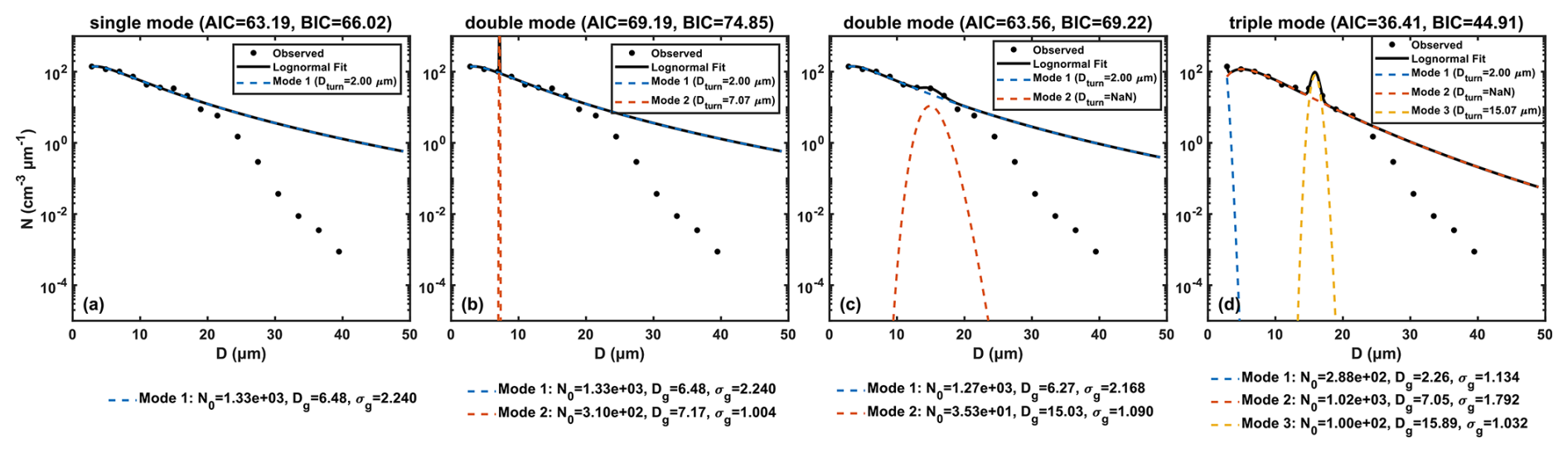
The following six representative examples are provided to illustrate the four candidate fits obtained for each individual DSD and the procedure by which the optimal fit is selected under the proposed criteria.

A2.1 Single mode examples

Figure A2 shows a unimodal DSD during the fog development stage prior to the maximum LWC in F1–1. The D_turn of mode 2, defined by the intersection between mode 1 and mode 2, falls within the same bin as the D_turn of mode 1 and is therefore considered invalid and shown as NaN in the figure. Despite the trimodal fit yielding the lowest AIC and BIC values, this fit is discarded. Consequently, the unimodal fit (panel a) with the second-lowest AIC and BIC values was selected to determine the number of modes in this DSD.

Figure A2 Example of single mode DSD.

A2.2 Double mode examples

Figure A3 shows the DSD during the fog development stage prior to the maximum LWC in F1–1, corresponding to the light-blue curve in Fig. 7b. For this DSD, the trimodal fit in panel (d) and the bimodal fit in panel (c) with lower AIC and BIC values were discarded because mode 1 and mode 2 do not intersect (appearing as NaN in the figure), making it impossible to determine the second mode. In the bimodal fit shown in panel (b), both modes 1 and 2 have corresponding D_turn that do not fall within the same or adjacent bins, and the sum of the AIC and BIC values is smaller than that of the unimodal fit. Therefore, this fit was used to determine the number of modes and the corresponding D_turn for this DSD.

Figure A3 Example 1 of double mode DSD.

Figure A4 Example 2 of double mode DSD.

Figure A5 Example 3 of double mode DSD.

Figure A6 Example 4 of double mode DSD.

Figure A7 Example of triple mode DSD.

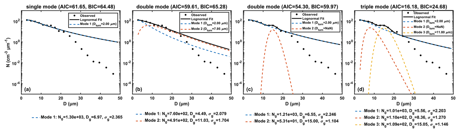
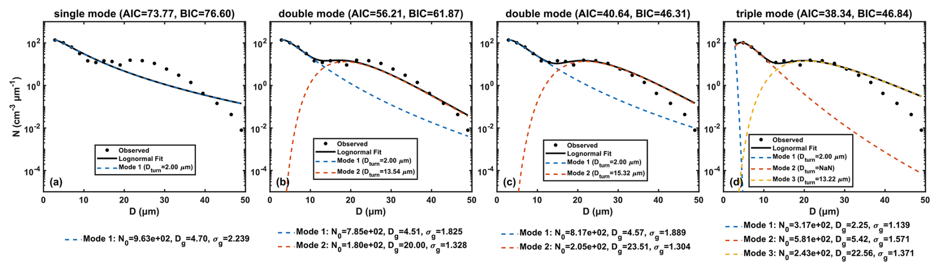
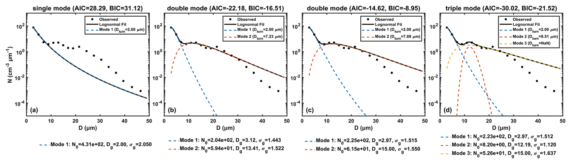
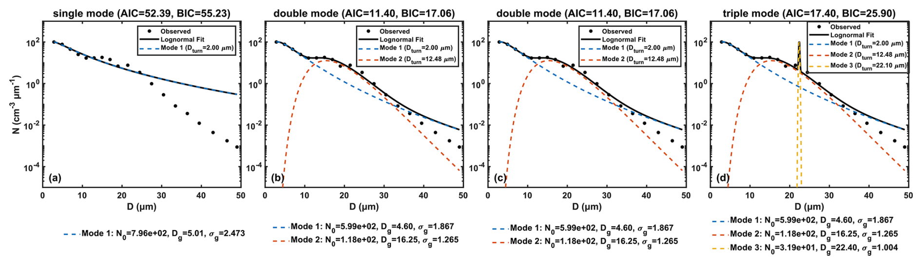
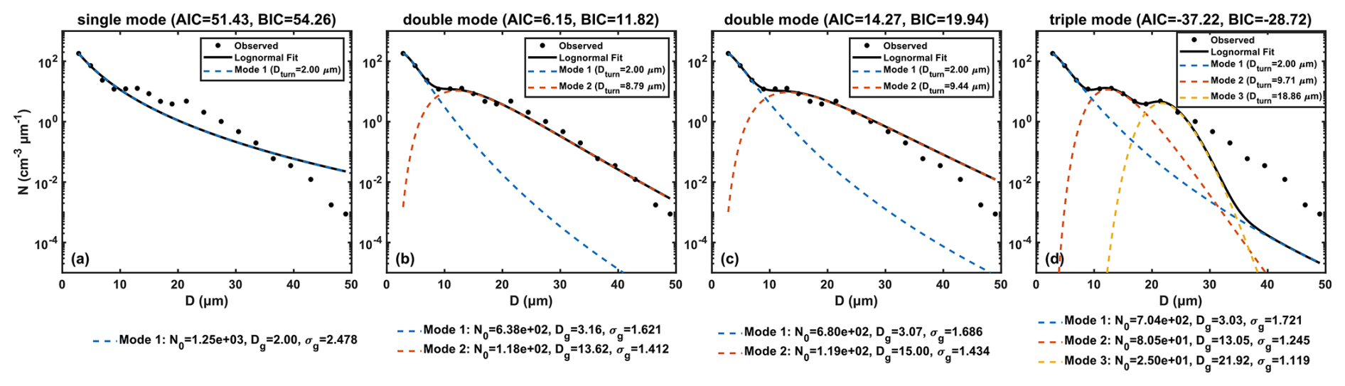
Figure A4 shows the DSD at the time when LWC in F1–1 reaches its maximum, corresponding to the purple curve in Fig. 7b. For this DSD, the trimodal fit (panel d) is discarded because the D_turn of the first and second mode fall within the same bin. Accordingly, the D_turn of mode 2 is shown as NaN in the figure. Among the remaining fits, the fit in panel (c) yields the lowest AIC and BIC values. The intersection between mode 1 and mode 2 defines a corresponding D_turn that does not fall within the same or adjacent bins. Therefore, the bimodal fit in panel (c), which has lower AIC and BIC values, is selected to represent the number of modes and the mode diameters of this DSD.

Figure A5 corresponds to the orange DSD in F10 prior to the maximum LWC (Fig. 8b). Compared with Fig. A7, this DSD exhibits a broader mode in the 10–25 µm size range. In the trimodal fit (panel d), mode 2 and mode 3 do not intersect, so the modes cannot be determined. This fit is therefore discarded, with the D_turn of mode 3 shown as NaN in the figure. The other three fits are all valid. Therefore, the bimodal fit in panel (c) with the smaller combined AIC and BIC is selected to determine the number of modes and the D_turn of this DSD.

Figure A6 corresponds to the green DSD in F1–1 prior to the maximum LWC (Fig. 7b). In the fitting procedure, D_g was constrained to 5–20 µm for panel (b) and to 15–20 µm for panel (c). For this DSD, the retrieved D_g falls within the overlapping range of the two parameter bounds (15–20 µm), resulting in identical fitting results in panels (b) and (c). Because they yield the lowest AIC and BIC values, and the corresponding D_turns do not fall within the same or adjacent bins, this DSD is classified as bimodal.

A2.3 Triple mode examples

Figure A7 shows the mode identification result for the yellow curve prior to the maximum LWC in F10 (Fig. 8b). In the trimodal fit (panel d), intersections exist between mode 1 and mode 2 as well as between mode 2 and mode 3, and the resulting D_turn satisfy the physical requirement that they do not fall within the same or adjacent bins. Moreover, this fit yields the minimum combined AIC and BIC among all fits. Therefore, it is used to define the number of modes and the D_turn of this DSD.

A3 MODIS 3.9 µm shortwave infrared and visible channel imagery for F1–1, F10, and F20

For F4 and F18, no satellite imagery is available within the fog period because the overpass times of the polar-orbiting satellite did not coincide with the observations.

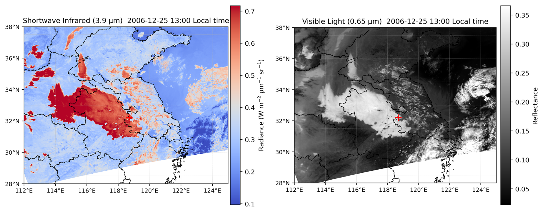
Figure A8 Aqua MODIS 3.9 µm shortwave infrared and visible channel imagery for Fog 1–1, with the observation site marked by a red cross. Satellite imagery from MODIS (Aqua), NASA LAADS DAAC. Administrative boundaries derived from the CN-border dataset, based on data from the National Catalogue Service For Geographic Information (https://www.webmap.cn, last access: 25 February 2026).

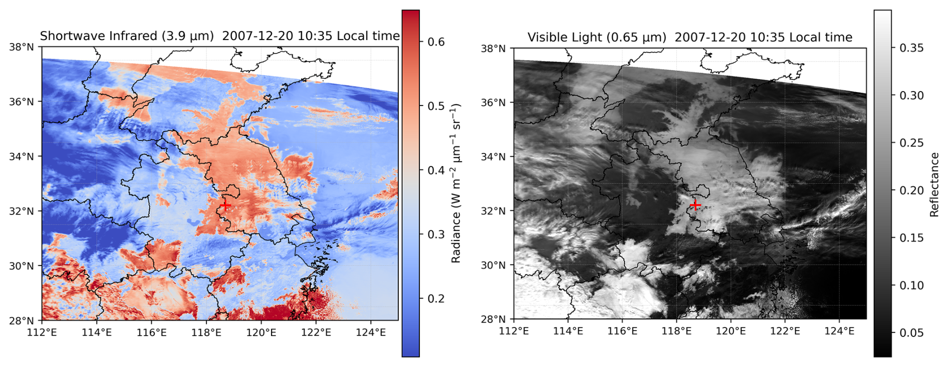
Figure A9 Terra MODIS 3.9 µm shortwave infrared and visible channel imagery for Fog 10, with the observation site marked by a red cross. Satellite imagery from MODIS (Terra), NASA LAADS DAAC; administrative boundaries from the CN-border dataset (National Catalogue Service For Geographic Information, https://www.webmap.cn).

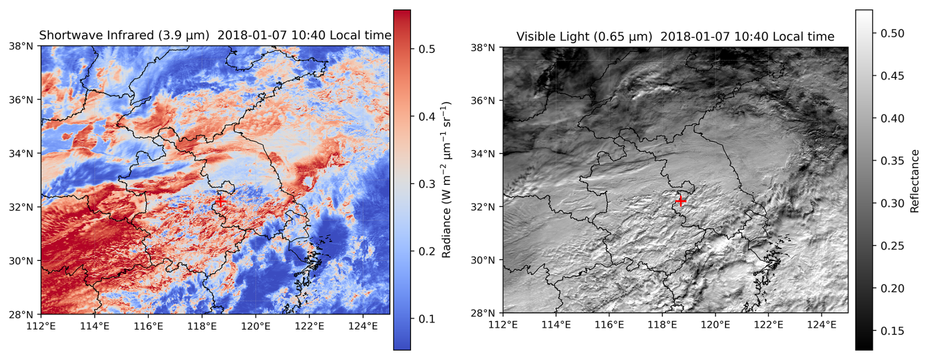
Figure A10 Terra MODIS 3.9 µm shortwave infrared and visible channel imagery for Fog 20, with the observation site marked by a red cross. Satellite imagery from MODIS (Terra), NASA LAADS DAAC; administrative boundaries from the CN-border dataset (National Catalogue Service For Geographic Information, https://www.webmap.cn).

A4 Summary table of the 27 fog events and details of fog type identification

In this study, some cases classified as radiation fog have initial times in the early morning rather than at night. For these less typical cases, additional details on the fog types identify are provided here. Fog case 6 formed during the night and dissipated around 06:00. According to the observation log, light mist persisted at the site until the formation of Fog case 7, but it did not meet the criteria used in this study to define fog (N_f>10 cm⁻³ and LWC > 10⁻³ g m⁻³). Therefore, Fog case 6 and Fog case 7 were treated separately, although their formation mechanisms were the same. For Fog case 8, the night preceding fog formation was clear, with strong radiative cooling and very weak winds, conditions favorable for fog development. Fog case 8 was therefore classified as a radiation fog. Fog case 26 developed in the morning. Light drizzle occurred the previous afternoon, followed by light mist during the night, indicating that precipitation played a role in its formation.

Table A1 Initial and end times, classification, visibility, meteorological variables (temperature, wind speed) and microphysical properties of the 27 fog events, the first row shows the mean values, in the parentheses are the 25th and 75th percentiles of each characteristic. In the first row of the column titled Modes, the DSD types observed in each case are listed, where U, D, and T denote unimodal, bimodal, and trimodal DSD, respectively.

A5 Additional figures to be included

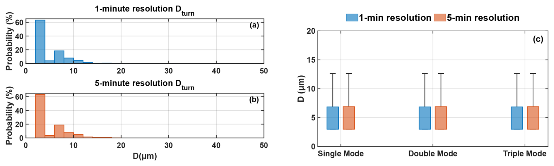
Figure A11 The D_turn distributions of all DSDs obtained using gamma distribution at 1 min resolution (a), 5 min resolution (b), and the D_turn distributions by DSD type at both resolutions (c).

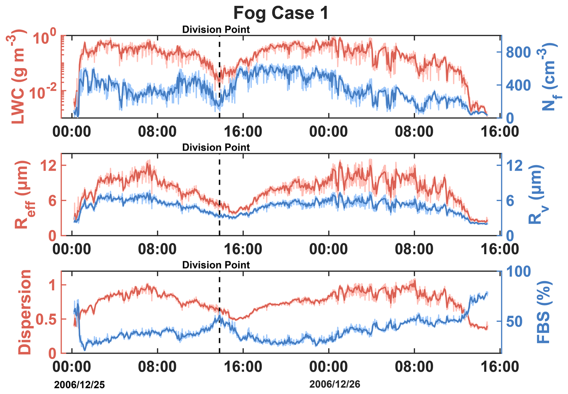
Figure A12 The temporal evolution of N_f, LWC, R_v, R_eff, FBS and ε for fog case 1, the dark lines represent 5 min averaged values while the light lines are 1 min averaged values, the black dashed line is the boundary between F1–1 and F1–2.

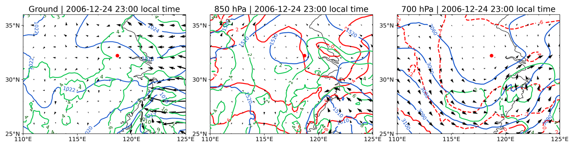
Figure A13 Synoptic conditions of Fog 1–1. Red dots indicate observation stations; blue lines represent isobars or geopotential height contours; red lines are isotherms, dashed when temperatures are below 0 °C; green lines denote constant specific humidity.

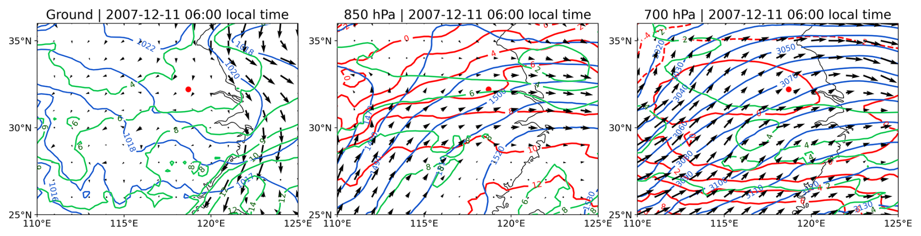
Figure A14 Synoptic conditions of Fog 4.

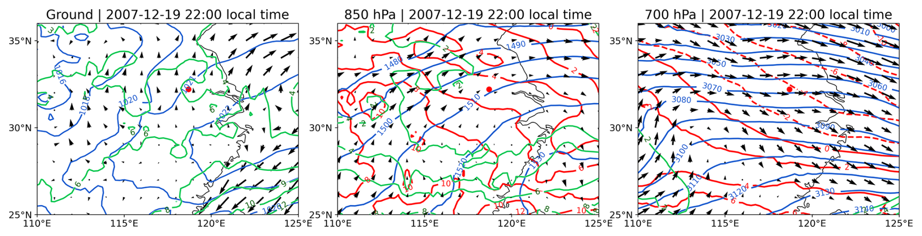
Figure A15 Synoptic conditions of Fog 10.

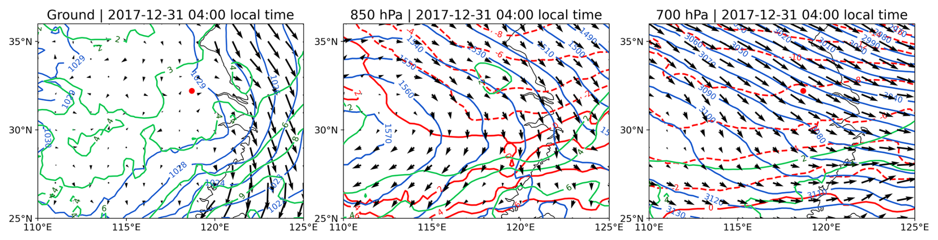
Figure A16 Synoptic conditions of Fog 18.

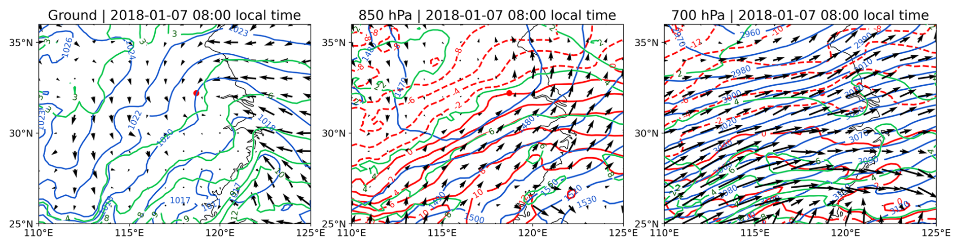
Figure A17 Synoptic conditions of Fog 20.

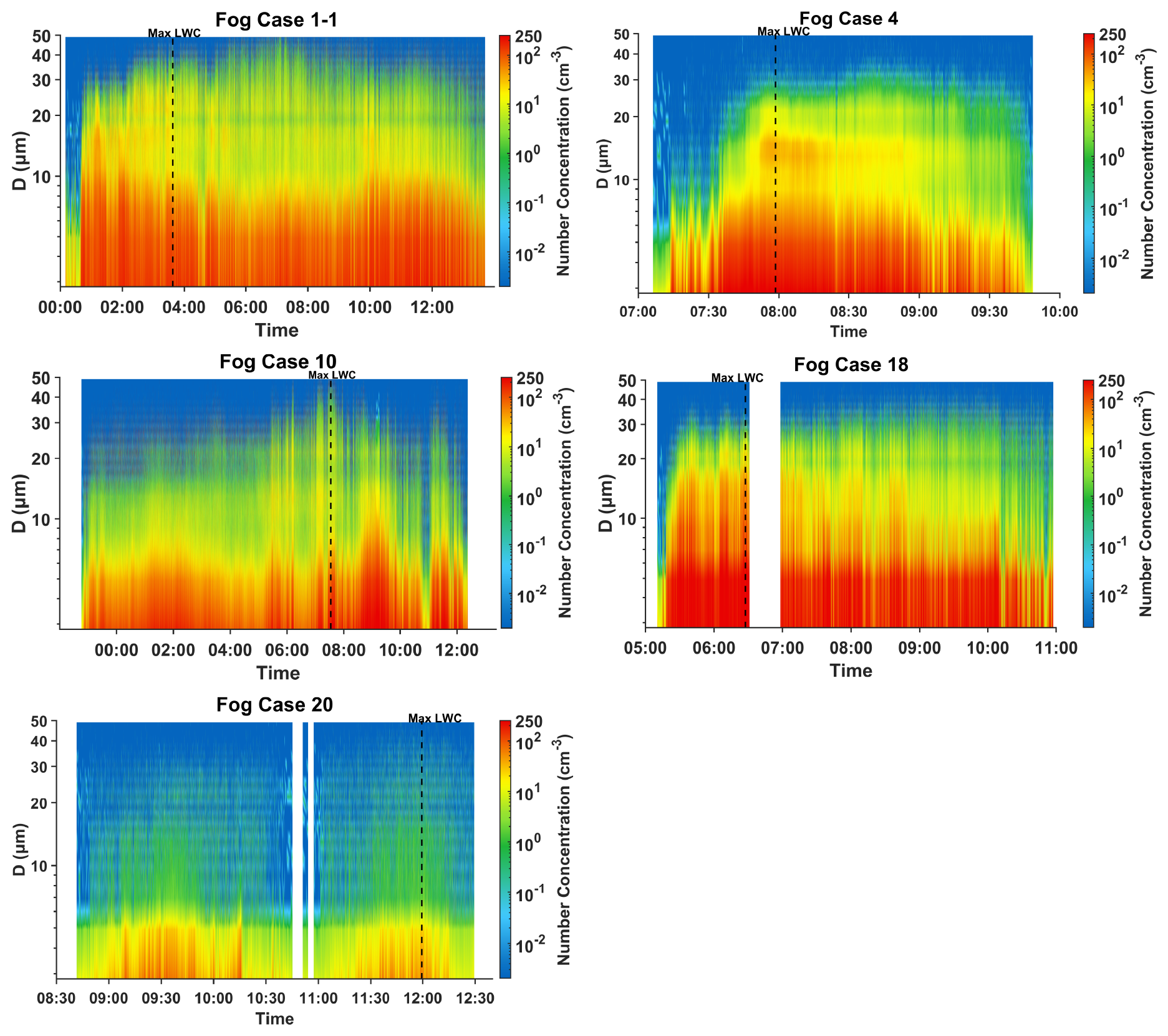
Figure A18 The time series of DSDs at 1s resolution of Fog Case 1–1, Fog Case 4, Fog Case 10, Fog Case 18 and Fog Case 20.

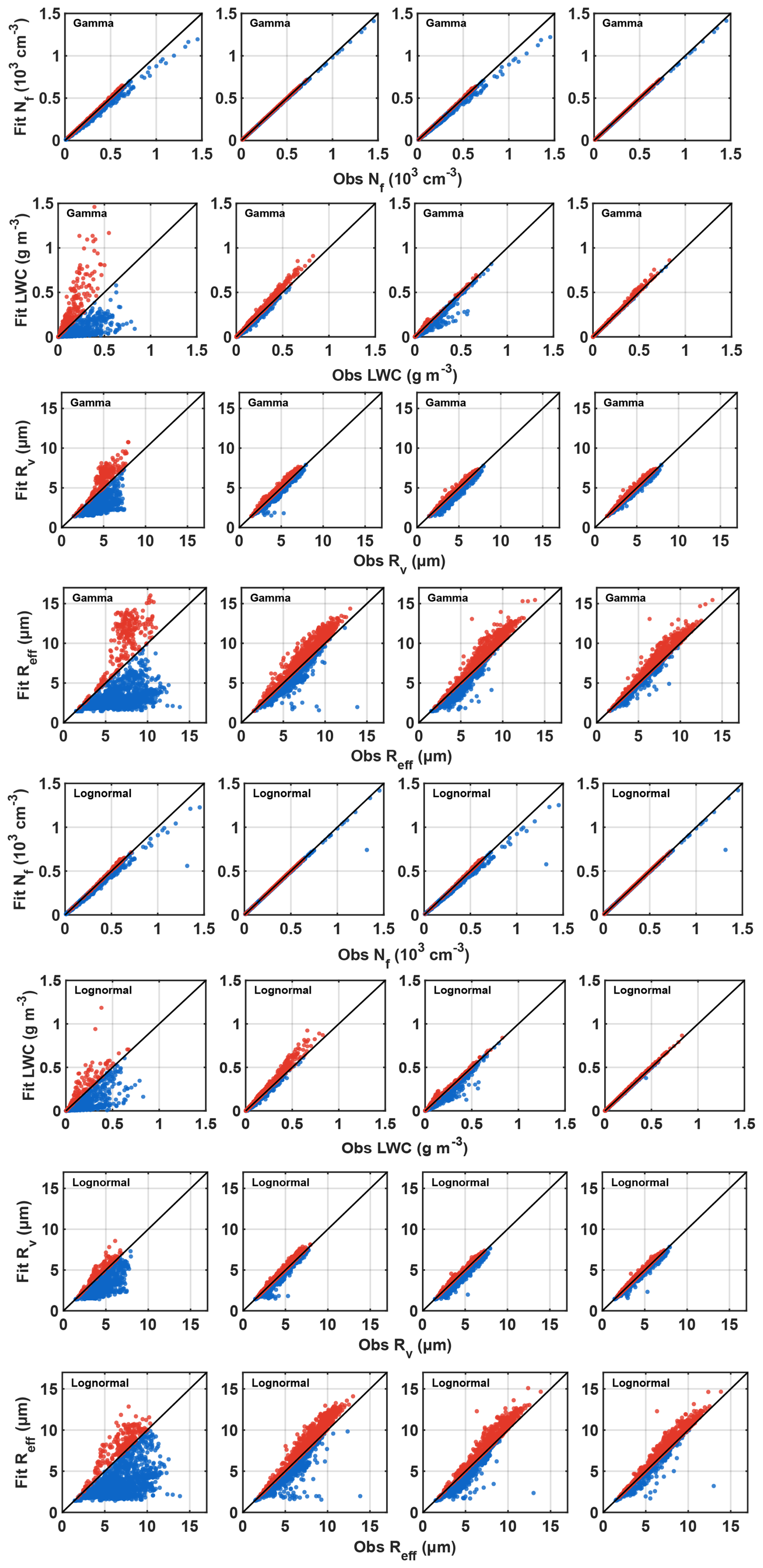
Figure A19 Correlation between N_f, LWC, R_v and R_eff derived from observed spectrum and those computed from the gamma and lognormal fitted spectrum with no breakpoint (first column), breakpoint at 10 µm (second column), breakpoint at 20 µm (third column) and breakpoint at 10 and 20 µm (fourth column). Red dots indicate overestimation of the microphysical properties by the gamma fit, while blue dots indicate underestimation.

A6 Discussion of the sensitivity of segmented gamma and lognormal fits to the exclusion of potential modes in 30–50 µm

To examine the impact of excluding potential modes in the 30–50 µm range on segmented gamma and lognormal fitting, an additional segmentation points at 40 µm was considered. Using the same approach as in Sect. 3.4, segmented fits were applied to all DSDs, and the fitting results were used to retrieve N_f, LWC, R_v, R_eff, absorption coefficient and optical thickness. The deviations of these retrieved quantities from the observations were then calculated. Figure A19 compares the deviations obtained from fits with segmentation points at 10 and 20 µm and those including the additional 40 µm segmentation point. The results show that introducing the 40 µm segmentation point does not lead to a significant improvement in fitting performance, indicating that the omission of potential modes larger than 30 µm does not substantially affect the results of this study.

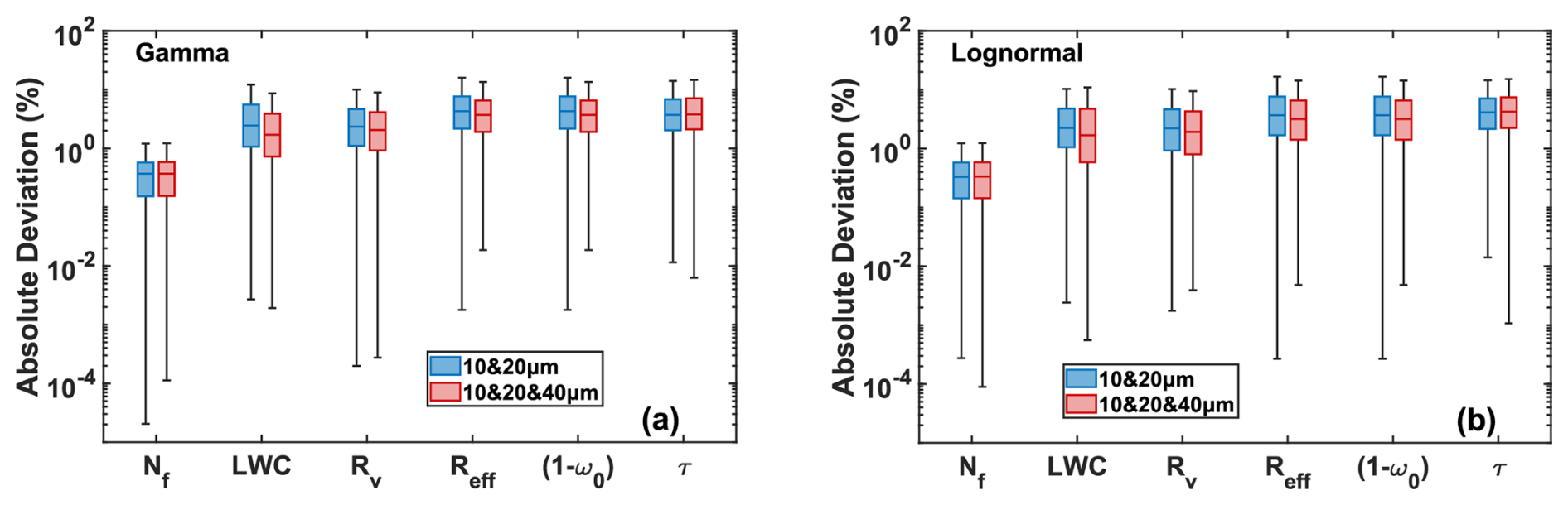
Figure A20 Comparison between segmented fitting results with breakpoints at 10 and 20 µm (a) and those with additional breakpoints at 10, 20, and 40 µm (b).