Northern Hemisphere stratospheric polar vortex morphology under localized gravity wave forcing: a shape-based classification

The Northern Hemisphere stratospheric polar vortex (SPV) response to localized gravity wave (GW) forcing remains poorly understood, particularly in terms of its detailed morphology. Here, we investigated geometry-specific impacts of enhanced orographic GW drag in three hotspot regions, the Himalayas, Northwest America, and East Asia, using ensemble simulations with the high-top UA-ICON global circulation model. By classifying daily SPV geometries into ten distinct clusters with a novel unsupervised, shape-based hierarchical clustering framework, we isolated geometry-specific responses using the class contribution method. Our results show that all hotspot forcings consistently reduce planetary wave 1 (PW1) amplitude and induce a PW1-like displacement of the SPV core, though spatial patterns vary with hotspot location. This response manifests as negative geopotential height (GPH) anomalies within the forced region and positive anomalies to the north, indicating localized SPV edge mixing. The response is also sensitive to the forcing’s latitudinal position: the Himalayas, as the southernmost hotspot, produces a deepened vortex, while the more poleward Northwest America and East Asia forcings show similar patterns with greater intrusion of positive GPH anomalies into the vortex core. The forcing reduces PW1 amplitude both by shifting the frequency of specific clusters and altering the mean structure of the most frequent classes. Our results demonstrate that shape-based clustering combined with the class contribution framework can reveal robust, spatially coherent signals that might otherwise be masked by internal variability, providing a new perspective for understanding SPV variability and its predictability.

1 Introduction

The stratospheric polar vortex in the Northern Hemisphere (SPV from now on) is a dominant cyclonic feature in the stratosphere that surrounds the winter pole (typically November to March), characterized by strong westerlies forming the polar night jet (Waugh et al., 2017). Compared to its Southern Hemisphere counterpart, the SPV exhibits greater variability due to stronger wave activity in the Northern Hemisphere, primarily driven by the extensive land-ocean contrasts and prominent orographic features (Waugh and Randel, 1999; Butchart, 2022). The variability of the SPV can substantially influence tropospheric weather and climate through downward coupling processes (Haynes et al., 1991; Baldwin and Dunkerton, 2001; Hardiman and Haynes, 2008; Hitchcock and Simpson, 2014; Kidston et al., 2015; Scaife et al., 2022).

Large-scale planetary waves (PWs) are one of the major drivers of the stratospheric dynamics (Andrews and Mcintyre, 1976). These waves significantly influence the state and morphology of the SPV (Waugh, 1997; Karpetchko et al., 2005; Günther et al., 2008; Albers and Birner, 2014). PWs typically have large horizontal scales – most commonly zonal wavenumber 1 (PW1) or 2 (PW2) – and can propagate vertically into the stratosphere, where they distort and decelerate the vortex (Riese et al., 2002). In essence, the stratospheric vortex’s general shape is a direct imprint of these waves. PW1 induces a single ridge–trough pattern, displacing the vortex off the pole, while PW2 generates two ridges and two troughs, elongating the vortex into an elliptical structure or even splitting it into two distinct lobes (Finke et al., 2025). The breaking of PWs in the stratosphere is broadly recognized as the main driver of sudden stratospheric warmings (SSWs), abrupt and significant rises in polar stratospheric temperatures during winter, associated with a decrease or even reversal of the typical zonal-mean westerly winds (Baldwin et al., 2021).

In addition to PWs, gravity waves (GWs) also play a crucial role in shaping wintertime stratospheric dynamics and the structure of the SPV by transferring momentum and energy upward from the troposphere to middle atmosphere regions where they dissipate (Andrews et al., 1987; Fritts and Alexander, 2003; Yiğit and Medvedev, 2016). GWs can originate from various sources, broadly categorized as orographic, generated by airflow over major mountain ranges (Smith, 1980; Nastrom and Fritts, 1992), and non-orographic, arising from processes such as deep convection, jet streams, frontal systems, and shear instabilities (Eckermann and Vincent, 1993; Alexander et al., 1995; Bühler et al., 1999; Plougonven and Zhang, 2014). GW activity exhibits a pronounced zonal asymmetry, with well-defined hotspot regions where GW amplitudes and associated momentum drag are particularly strong (Ern et al., 2004; Fröhlich et al., 2007; Hoffmann et al., 2013; Schmidt et al., 2016). These hotspots are typically episodic and intermittent in nature and are commonly linked to prominent orographic regions such as the Himalayas, the North American Rockies, and East Asia (Hertzog et al., 2012; Hoffmann et al., 2013; Wright et al., 2013; Šácha et al., 2015; Kuchar et al., 2020; Gupta et al., 2024; Hozumi et al., 2024).

The location and distribution of GW drag exert a strong influence on the state of the SPV (Samtleben et al., 2019, 2020a, b; Kuchar et al., 2020; Sacha et al., 2021; Mehrdad et al., 2025a). GWs can affect the SPV by modulating PW behavior in the stratosphere through mechanisms collectively referred to as “compensation mechanisms” (Cohen et al., 2013, 2014; Sigmond and Shepherd, 2014; Karami et al., 2022). Among these compensation mechanisms is the ability of GW drag to disrupt the vortex edge and locally generate PW activity at breaking regions, thereby reshaping the SPV (Coy et al., 2024). The extent of GW influence on stratospheric dynamics is highly sensitive to the spatial and temporal patterns of the resulting GW drag (Boos and Shaw, 2013; Shaw and Boos, 2012; Šácha et al., 2016; Kuchar et al., 2020), with a particularly strong dependence on how the GW drag aligns in phase with PWs (Samtleben et al., 2019, 2020a; Mehrdad et al., 2025a).

The SPV morphology and GW forcing are tightly coupled. Differences in GW parameterizations are a major driver of inter-model spread in stratospheric dynamics, manifesting in both the frequency and type of SSWs and in the morphology of the SPV itself (Sigmond et al., 2023; Kuchar et al., 2024). The instantaneous shape of the vortex filters and redistributes GW momentum, altering the background wind and temperature fields that GWs encounter (Andrews et al., 1987). In turn, zonally asymmetric GW drag feeds back on the SPV, modifying its shape and dynamical behavior (Coy et al., 2024; Kuchar et al., 2024). Despite growing evidence that regional GW hotspots modulate the middle atmospheric dynamics (Šácha et al., 2016; Samtleben et al., 2019, 2020a; Kuchar et al., 2020; Sacha et al., 2021), their geometry-specific and climate-scale impacts on the SPV remain poorly quantified. These impacts are particularly important because the zonally asymmetric nature of GW forcing means that its dynamical effects on the SPV can vary significantly depending on the underlying SPV geometry and state. Previous studies have documented the atmospheric response to enhanced GW drag in hotspot regions within a zonal-mean framework (Samtleben et al., 2020a; Kuchar et al., 2020; Sacha et al., 2021), but none have systematically examined this response in the context of SPV morphology. Such a perspective is critical, as the SPV's structure governs downward coupling to the troposphere and influences the likelihood of extreme events such as SSWs (Baldwin and Dunkerton, 2001; Charlton and Polvani, 2007; Seviour et al., 2013; Messori et al., 2022; Ding et al., 2023).

Mehrdad et al. (2025a) used the high-top UA-ICON (ICOsahedral Nonhydrostatic model with Upper-Atmosphere extension) to run ensemble experiments with regionally intensified subgrid-scale orographic (SSO) GW drag over three Northern Hemisphere hotspots (Himalayas, Northwest America, and East Asia). They found a coherent hemispheric response in which resolved waves compensated the localized drag, suppressing primarily PW1 propagation and strengthening upper-stratospheric/mesospheric westerlies, with a region-dependent influence on SSW frequency. Here, we built on the experiments of Mehrdad et al. (2025a) but extended the analysis in three pivotal ways. (i) We implemented a hierarchical unsupervised, shape-based classification that categorizes the daily SPV state into ten distinct geometry-based clusters. (ii) We Leveraged the class-contribution framework introduced by Mehrdad et al. (2024), along with ensemble-based analysis, to isolate the characteristic patterns through which enhanced GW hotspot forcing modifies the SPV, distinguishing them from internal variability. (iii) We investigated how these geometry-conditioned responses feed back onto broader stratospheric dynamics. By focusing on SPV morphology, this approach extends the zonal-mean analysis of Mehrdad et al. (2025a), offering a new lens through which to understand the influence of non-zonal GW forcing on Northern Hemisphere stratospheric variability.

2 Data and methodology

This section outlines the simulation setup, datasets, and analysis procedures used in this study.

2.1 Model simulations

We employed the same set of ensemble climate simulations as described in Mehrdad et al. (2025a), using the upper-atmosphere configuration of the ICON general circulation model (UA-ICON; Borchert et al., 2019). UA-ICON is a high-top model that extends well above the stratopause and features fine vertical resolution, meeting the requirements for realistically simulating SPV behavior (Wu and Reichler, 2020; Zhao et al., 2022; Kuchar et al., 2024). The model has been shown to realistically represent stratospheric dynamics and key aspects of wave-driven troposphere–stratosphere coupling (Köhler et al., 2023; Kunze et al., 2025; Mehrdad et al., 2025a). The simulations were performed with the R2B4 grid (approximately 160 km horizontal resolution), 120 vertical levels extending up to 150 km, and were driven by annually repeating present-day (1979–2022) climatological boundary conditions. The simulations were initialized with the mean atmospheric state on 1 January, derived from the 1979–2022 ERA5 climatology, representing the present-day climatological mean.

To investigate the impact of regionally intensified orographic GW forcing, we conducted a control simulation (C) and three sensitivity experiments. The control run used the default model configuration. In the sensitivity experiments, the GW drag produced by the SSO scheme (Lott and Miller, 1997) was enhanced by a factor of 10 in three GW hotspot regions – the Himalayas (HI), Northwest America (NA), and East Asia (EA) – while the low-level component of the SSO drag, associated with flow blocking and wake effects, remained unchanged. The forced regions are defined as follows: EA spans 30–60° N and 110–175° E; NA spans 30–60° N and 100–130° W; and HI spans 25–45° N and 70–100° E. Each experiment, including the control run, comprises a six-member ensemble of 30-year simulations under identical boundary conditions. The ensemble members were generated by perturbing the initial conditions. A concise summary of the exerted SSO zonal drag across hotspots is provided in Appendix A (Figs. A2 and A1). For full details on the model configuration, ensemble design, and GW forcing strategy, see Mehrdad et al. (2025a) and the accompanying publicly available datasets (see Code and data availability section).

2.2 Data

In this study, we analyzed daily model output for the extended boreal winter season (November through March, NDJFM), focusing exclusively on the Northern Hemisphere, considering data poleward of 0° latitude. Daily values were computed as the average across all model time steps within each simulation day. The first year of each simulation was considered as the model spin-up time and was therefore excluded from the analysis.

To characterize the stratospheric polar vortex, we used the geopotential height (GPH) field at the 10 hPa level. These GPH fields were interpolated onto a Lambert azimuthal equal-area projection centered on the North Pole (Snyder, 1987), using a horizontal grid spacing of 1.5°, which closely matches the native resolution of the model. We also used temperature and horizontal wind fields to derive zonal-mean quantities and Eliassen–Palm (EP) flux and its divergence (Andrews et al., 1987).

2.3 Classification of SPV geometry

The morphology of the SPV encodes much of its dynamical state and mediates where and how PWs and GWs interact with it. Prior work has mainly followed two approaches for evaluating the SPV morphology. One uses geometric feature extraction to summarize the vortex with a few diagnostics, such as centroid latitude, aspect ratio, or equivalent area, thereby enabling split/displacement identification and basic morphology tracking (Mitchell et al., 2013; Seviour et al., 2013). These diagnostics are transparent but necessarily coarse, and they cannot capture higher-order shape attributes such as skewness, curvature variations, or non-elliptical deformations. The other approach applies field-based clustering on wind or other dynamical fields, providing a holistic view of the flow structure (Kretschmer et al., 2018). However, such gridpoint-wise similarity measures are typically blind to the spatial relationships among grid points and are sensitive to small translations and rotations of the vortex, so two vortices with nearly identical shapes but slightly different positions may appear far apart in feature space.

Here, we combine the strengths of both approaches by classifying the geometry of the SPV boundary using a representation based on Fourier descriptors. This representation encodes the boundary as a compact, physically interpretable set of coefficients. Low-order harmonics quantify global shape properties, such as circularity, elongation, and orientation, while higher orders capture finer deformations. By retaining only the leading modes, we emphasize large-scale morphology and suppress small-scale variability, yielding a low-dimensional yet expressive feature space. In this space, vortices with similar geometries (even under modest displacement or rotation) tend to cluster together, enabling a stable and physically meaningful morphology-based classification that is less sensitive to spatial shifts than gridpoint-wise approaches, yet far richer than scalar shape metrics.

We then analyzed the impact of regional GW hotspots on the SPV geometry. The workflow proceeds in three steps. First, we extracted daily SPV boundaries from 10 hPa geopotential height fields. Second, we constructed a compressed geometric feature space by computing the complex boundary signal and its Fourier descriptors, retaining only the leading modes. Third, we performed unsupervised hierarchical clustering (Ward linkage) on these descriptors to obtain discrete SPV geometry classes. In the following subsections, we provide a detailed explanation of each step in this process.

2.3.1 SPV boundary detection and feature extraction

The vortex boundaries were extracted from the daily 10 hPa GPH fields of all simulations during the extended winter period (see an example in Fig. 1). We retained only data northward of 25° N, as our analysis focuses on the SPV located in the Northern Hemisphere extratropics. For each daily field, we defined the SPV boundary as the contour enclosing the lowest 18 % of GPH values (i.e., the 18th percentile of that day’s GPH distribution), shown by the white line in the left panel of Fig. 1. The 18 % threshold was chosen empirically to capture a suitable range of vortex geometry.

Next, we defined each closed boundary in the daily field with more than 10 boundary pixels as an SPV boundary object. A daily field could therefore contain zero, one, or multiple boundary objects. For each SPV boundary object identified in a daily field, we extracted Fourier descriptors (Zahn and Roskies, 1972; Persoon and Fu, 1977) as follows:

1. Forming the complex signal. We treated the two-dimensional boundary coordinates (x_k,y_k) in the projected system as a complex signal,

   $$\begin{array}{}\text{(1)}& z_k=x_k+i{y}_k,\end{array}$$

   where i is the imaginary unit and $k=\mathrm{1},\mathrm{\dots },N$ indexes the boundary pixels along the closed contour.

2. Applying the FFT. We performed a Fast Fourier Transform (FFT) (Cooley and Tukey, 1965) on this complex signal to obtain its Fourier coefficients. We then discarded the DC component (the zero-frequency term) and retained only the 10 largest remaining coefficients. All other coefficients were set to zero. The previously introduced limit of 10 boundary pixels ensures that each object is sufficiently large to be meaningfully represented by 10 harmonics.

3. Storing Fourier Descriptors. Because each of the 10 retained coefficients is complex, we stored the respective real and imaginary parts as 20 real values as the Fourier descriptors (Zahn and Roskies, 1972; Persoon and Fu, 1977).

In addition to the 20 Fourier descriptors, we recorded:

• Boundary size. The total number of boundary pixels.

• Mass center. The center of the boundary object, reported as (x_center,y_center).

• Time feature. The relative day of the season with respect to January 1 (e.g., 1 November is −61, 10 January is +9, etc.).

For each SPV boundary object, we therefore derived a feature vector comprising a total of 24 features. The first two features represent the coordinates of the vortex center, the third feature encodes time, features 4 to 23 consist of 20 Fourier descriptors, and the final feature represents the boundary size. Since the focus of this analysis is the SPV shape, we did not include a feature directly representing the strength or depth of the vortex.

The constructed 24-dimensional feature space provides a compressed yet rich representation of the SPV state. The Fourier descriptors primarily capture the overall geometry of the vortex boundary. Lower-order harmonics encode global shape attributes, such as circularity versus elongation, while their phases indicate boundary orientation. The boundary size reflects the spatial extent of the vortex, the center encodes its location in a polar projection, and the time feature captures seasonal progression.

Moreover, by performing an inverse FFT with only the retained 10 largest coefficients (excluding the DC component) and translating the result according to the boundary’s mass center, we can reconstruct a smoothed representation of the original boundary (see the red line in the right panel of Fig. 1). This reconstruction illustrates how the features effectively capture the main structure of the SPV boundary object.

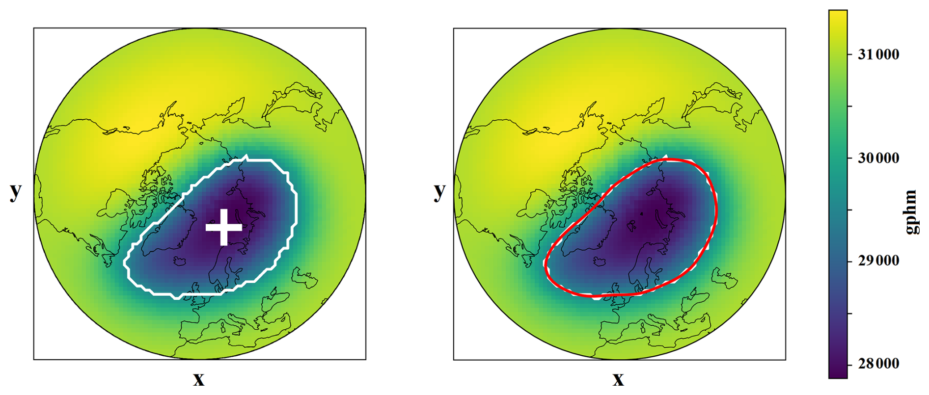
Figure 1 Geopotential height (GPH) fields at 10 hPa in GPH meters for a single day (19 February of the second year after the simulation start, corresponding to time feature +49) from the control simulation ensemble 1, shown in a Lambert azimuthal equal-area projection. The x and y axes represent the projection coordinates. The vortex boundary, defined as the lowest 18th percentile of the field values, is outlined with a white line in both panels, while the vortex center of mass (x_center,y_center) is indicated by the white cross in the left panel. The right panel also shows the reconstructed vortex boundary, derived from the extracted features, represented by the red line.

Note that, before performing any clustering or classification, we do not normalize the Fourier descriptors to preserve information about both scale and geometry. However, we rescale the (x_center,y_center) coordinates of the boundary center to match the maximum variance among all features in the dataset. Specifically, we calculate the variance of each individual feature across the whole dataset and identify the maximum variance. The central coordinate features are then normalized to have the same variance as this maximum. This adjustment ensures that the location of the boundary center has a comparable influence on the feature space as we employed Euclidean distance-based unsupervised classification. By doing so, we emphasize the role of boundary location in the clustering process.

2.3.2 SPV classification

We devised a hierarchical scheme to classify daily SPV states at 10 hPa. First, we categorized the daily data points based on the number of distinct SPV boundary objects in each daily field. Daily fields containing either zero or more than two SPV boundary objects were classified as unstable SPV and assigned to a global cluster labeled C1. This initial partitioning left two remaining categories for further analysis: single-SPV (exactly one boundary object) and split-SPV (exactly two boundary objects). Within each of these categories, we then applied hierarchical clustering using Ward's method (Ward, 1963; Johnson, 1967), which iteratively merges clusters to minimize the increase in within-cluster variance.

In the single-SPV category, each daily field is represented by a 24-dimensional feature vector. We computed the Euclidean distance in this 24-dimensional space to construct the pairwise distance matrix, a prerequisite for Ward's linkage criterion. The resulting dendrogram, shown in the upper panel of Fig. 2, is truncated to highlight the last 50 merges. A visual inspection revealed a distinct gap at approximately 12.5×10⁴ on Ward's linkage axis. Cutting the dendrogram at this level yielded five well-separated clusters, labeled C2–C6.

For the split-SPV category, each daily field contains exactly two SPV boundary objects, each represented by a 24-dimensional feature vector. Before computing distances between any two daily fields, we matched the boundary objects by identifying the closest pair of mass-center coordinates (x_center, y_center). Then, we computed the Euclidean distance between these matched objects in the 24-dimensional feature space, repeated this for the second pair of objects, and finally took the mean of the two object-wise distances as the distance between the two daily fields. We applied Ward's hierarchical clustering to these pairwise distances, and the resulting dendrogram is shown in the lower panel of Fig. 2. A threshold of 6×10⁴ yields four well-separated clusters (C7–C10). Thus, our classification framework partitions the SPV states into one unstable-vortex cluster (C1), five single-SPV clusters (C2–C6), and four split-SPV clusters (C7–C10). These clusters characteristics are elaborated in Sect. 3.2.

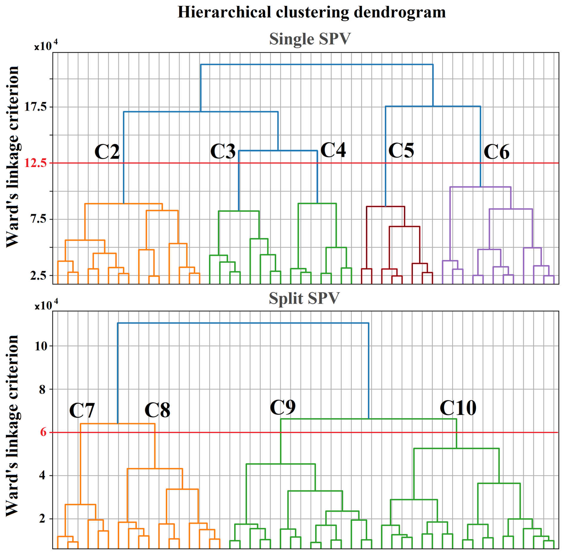
Figure 2 Hierarchical clustering dendrograms (Ward, 1963) displaying the last 50 merging steps for the single vortex category (upper panel) and the split vortex category (lower panel). The horizontal axis represents subsets of data points within each cluster branch, while the vertical axis shows Ward's linkage criterion (i.e., the increase in within-cluster variance based on Euclidean pairwise distances in feature space) at which clusters merge. Red horizontal lines in both panels represent thresholds of 12.5×10⁴ (upper panel) and 6×10⁴ (lower panel), which were used to partition the data into five clusters for the single vortex category and four clusters for the split vortex category, respectively. The cluster IDs (C2–C6 and C7–C10) are labeled at the intersection of the branches with the selected thresholds in both panels. Branches are colored (independently in each panel) to distinguish different merging routes and cluster heritage.

2.4 Class contribution

Class contribution quantifies the influence of different clusters – here, clusters of SPV – on anomalies in climatic parameters (Mehrdad et al., 2024). The sum of class contributions across all clusters in a sensitivity simulation yields the total anomaly of a given parameter. Each cluster's class contribution consists of two main components: Within-Cluster Variability Contribution (WCVC) and Frequency-Weighted Seasonal Deviation Contribution (FSDC). The WCVC represents how changes in the mean spatial characteristics of a cluster, such as minor shifts in its geometry or location, contribute to anomalies under the applied forcing in a sensitivity simulation. In contrast, the FSDC captures how variations in the occurrence frequency of a cluster influence the overall anomaly. Together, these components help differentiate whether observed anomalies arise from internal structural changes within a cluster (WCVC) or shifts in its prevalence (FSDC) in response to external forcing. A detailed methodological formulation is provided in Mehrdad et al. (2024).

3 Results

In this section, we first present the climatology of the control run, followed by the climatological differences in key climate variables between the control and sensitivity experiments. We then analyze the class centers and their associated mean states, and describe changes in the occurrence frequency across the different experiments. Finally, we assess the contribution of each class to the anomalies observed in key climate variables.

3.1 Climatology of the control and sensitivity experiments

Figure 3a shows the climatology of GPH at 10 hPa from the control run, along with the reconstructed SPV boundary based on the mean feature space of the control simulation. The climatological SPV exhibits an elliptical shape, with its center displaced toward northern Eurasia, consistent with previous findings based on reanalysis data (Kuchar et al., 2024). Figure 3b–d illustrate the GPH anomalies at 10 hPa for the HI, NA, and EA sensitivity experiments, respectively, relative to the control run. The dotted regions indicate where the ensemble mean differences are consistent in sign across at least five out of six ensemble members, which we refer to as the consistency criterion throughout the manuscript. All sensitivity experiments show a displacement of the SPV toward North America, although the magnitude of this shift varies among the experiments. The HI experiment exhibits the most pronounced and consistent shift. A similar pattern is evident in the potential vorticity (PV) anomalies on the 850 K isentropic surface, as shown in Fig. B1.

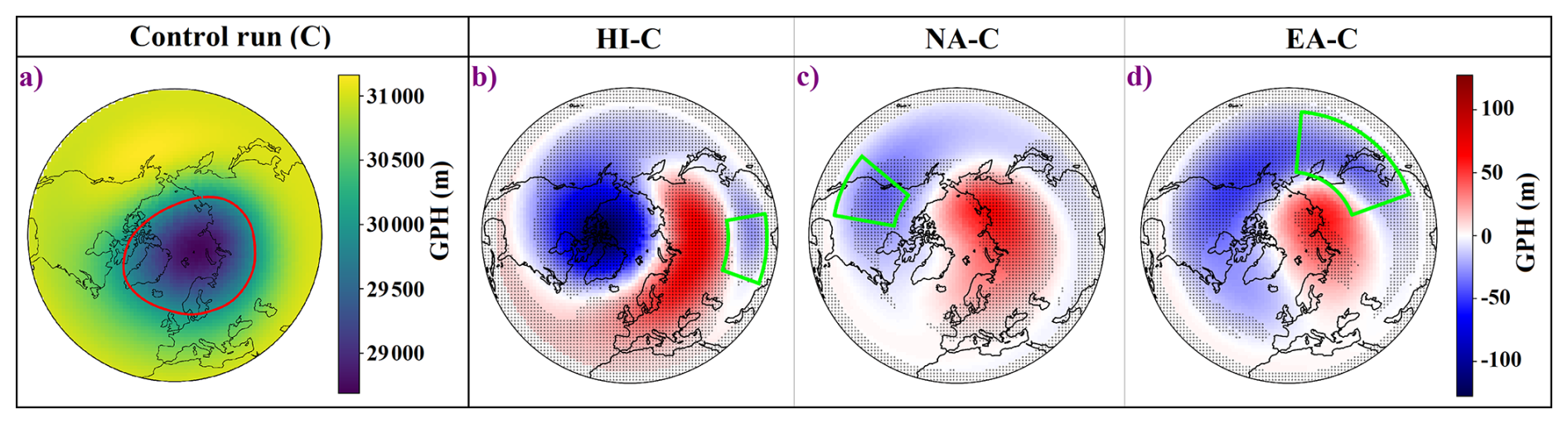
Figure 3 (a) Climatology of GPH at 10 hPa from the control run for the extended winter season (NDJFM). The red contour in panel (a) indicates the climatological reconstructed SPV boundary. Panels (b)–(d) show GPH anomalies for the HI, NA, and EA sensitivity experiments, respectively, relative to the control run, based on ensemble means. Dotted regions in panels (b)–(d) indicate areas where the anomalies are considered consistent, i.e., at least five out of six ensemble members exhibit the same anomaly sign as the ensemble mean. The green outlines indicate the forced regions in each sensitivity experiment.

Figure 4 presents the climatological structures and anomalies of PW1 (top row) and PW2 (bottom row) based on 10 hPa GPH fields. Cyan contours in panels (a)–(c) and (e)–(g) represent the climatological PW1 and PW2 patterns from the control run. PW1 is characterized by a high-pressure ridge over the North Pacific and North America and a corresponding low-pressure trough over Eurasia and the North Atlantic, whereas PW2 shows two ridge centers over the Alaska–Chukchi Sea region and Northern Europe/Scandinavia (Labitzke, 1981; Andrews et al., 1987).

In all sensitivity experiments, the imposed forcings act against the climatological PW1 pattern (Fig. 4a–c), resulting in a reduction of PW1 amplitude across mid- to high latitudes in the Northern Hemisphere (panel d). This amplitude reduction is strongest in the HI experiment and is consistent across most mid- to high latitudes in both the HI and EA experiments. In contrast, the NA experiment shows consistent amplitude reduction only near the latitudinal edge of the forcing region. Additionally, all experiments induce an eastward (positive) phase shift in PW1, which is consistent at high latitudes in the HI and NA experiments, and at lower latitudes in the HI and EA experiments.

For PW2 (Fig. 4e–h), the dominant response is again a reduction in amplitude. This reduction is strongest and most spatially consistent in the EA experiment, while in NA it is only partially consistent in the southern portion of the forcing latitudinal range. The HI experiment shows consistent amplitude reductions at low and mid-latitudes, but consistent increases at higher latitudes. Across all experiments, a westward phase shift is observed at lower latitudes (consistent in HI and NA), while an eastward and more consistent shift occurs at higher latitudes.

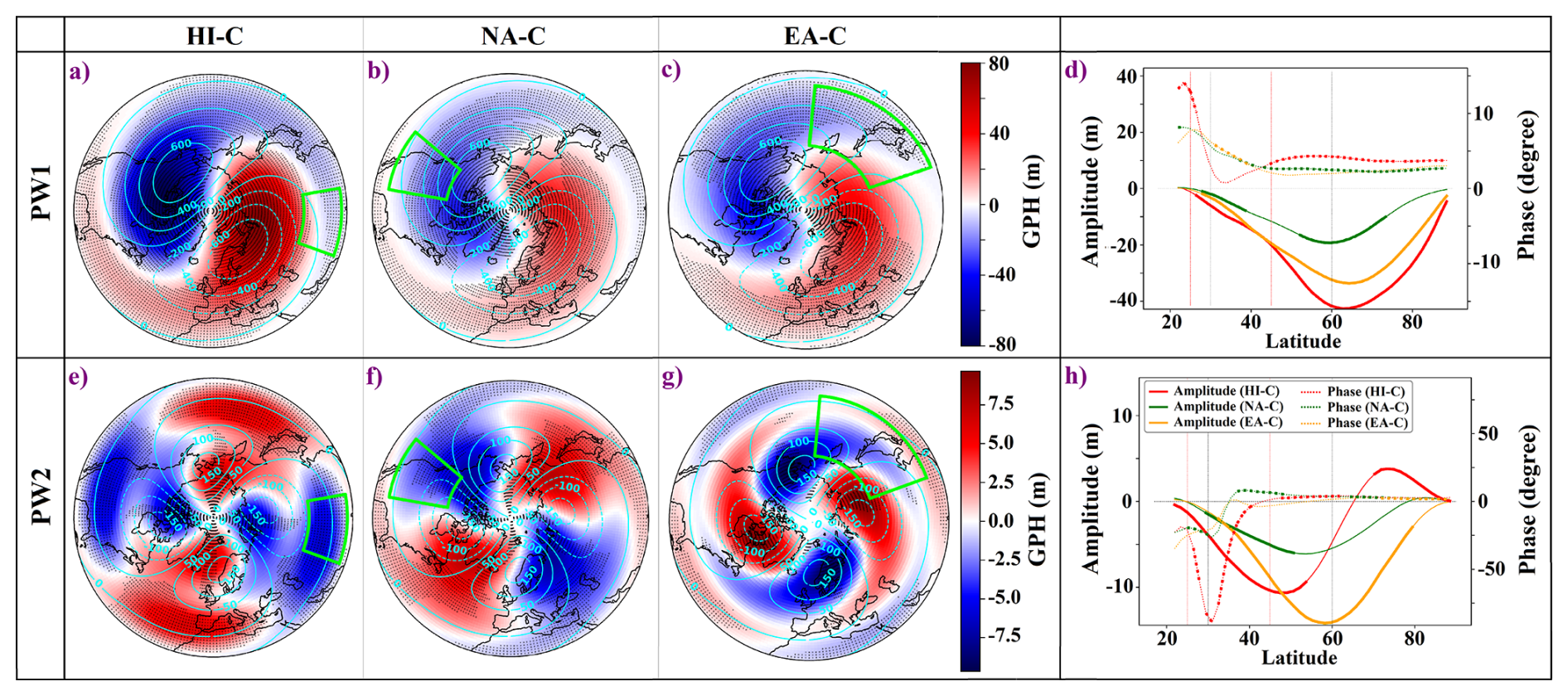
Figure 4 Climatology and anomalies of PW1 (top row, a–d) and PW2 (bottom row, e–h) calculated from 10 hPa GPH fields. Panels (a)–(c) show PW1 anomalies for the HI, NA, and EA simulations, respectively, with color shading. The corresponding PW1 climatology from the control run is overlaid in cyan contours. Panels (e)–(g) show PW2 anomalies for the same experiments, also with overlaid control run climatology. Anomalies are based on ensemble means, and dotted regions indicate areas where the anomaly are consistent across ensemble members. Panels (d) and (h) present the latitudinal profiles of PW1 and PW2 amplitude (solid lines, left y axis) and phase (dotted lines, right y axis) anomalies, respectively, for each sensitivity simulation relative to the control run. Note the different scaling for PW1 and PW2. Thicker segments indicate latitudes where the anomalies are consistent across ensemble members. Vertical dashed lines (d, h) in red mark the latitudinal extent of the forcing region in the HI experiment, while dashed black lines denote the forcing regions for the NA and EA experiments.

A reference climatology of the zonal-mean zonal wind and EP flux divergence is provided in Appendix C (see Fig. C1). Figure 5 shows anomalies in the zonal-mean zonal wind (panels a–c) and EP flux divergence (panels d–f) for each sensitivity experiment, relative to the Control run. All sensitivity experiments exhibit a deceleration of the stratospheric westerlies associated with the imposed forcing (see Fig. A2), extending poleward from the forcing regions (panels a–c). This is accompanied by a general positive EP flux divergence anomaly in the stratosphere (panels d–f), meaning the divergence is reduced relative to the control run, which indicates weaker wave drag (Mehrdad et al., 2025a). The decomposition of the EP flux divergence anomalies into leading zonal planetary wave modes revealed that the resolved response is dominated by PW1 (Mehrdad et al., 2025a).

In the HI experiment (Fig. 5a and d), westerlies increase consistently throughout the stratosphere at high latitudes, while EP flux divergence anomalies are consistently positive across the midlatitudes and in the high-latitude upper stratosphere, indicating a reduction in wave drag. In contrast, consistent negative EP flux divergence anomalies are observed in the lower to mid stratosphere at high latitudes, implying enhanced wave drag. In the NA experiment (panels b and e), zonal-mean zonal winds exhibit a consistent reduction of the westerlies across the midlatitudes, accompanied by the corresponding consistent positive EP flux divergence anomalies in the same region. In the EA experiment (panels c and f), westerlies increase consistently equatorward of around 40° N but show a consistent decrease north of around 45° N. EP flux divergence anomalies are consistently positive in both mid- and high-latitude regions, with weak but consistent negative anomalies in the lower stratosphere. We note that in all experiments, the zonal wind decrease related to and poleward of the GW forcing region is accompanied by a decreasing westward PW forcing, which is outweighed by the GW mean wind forcing (Mehrdad et al., 2025a).

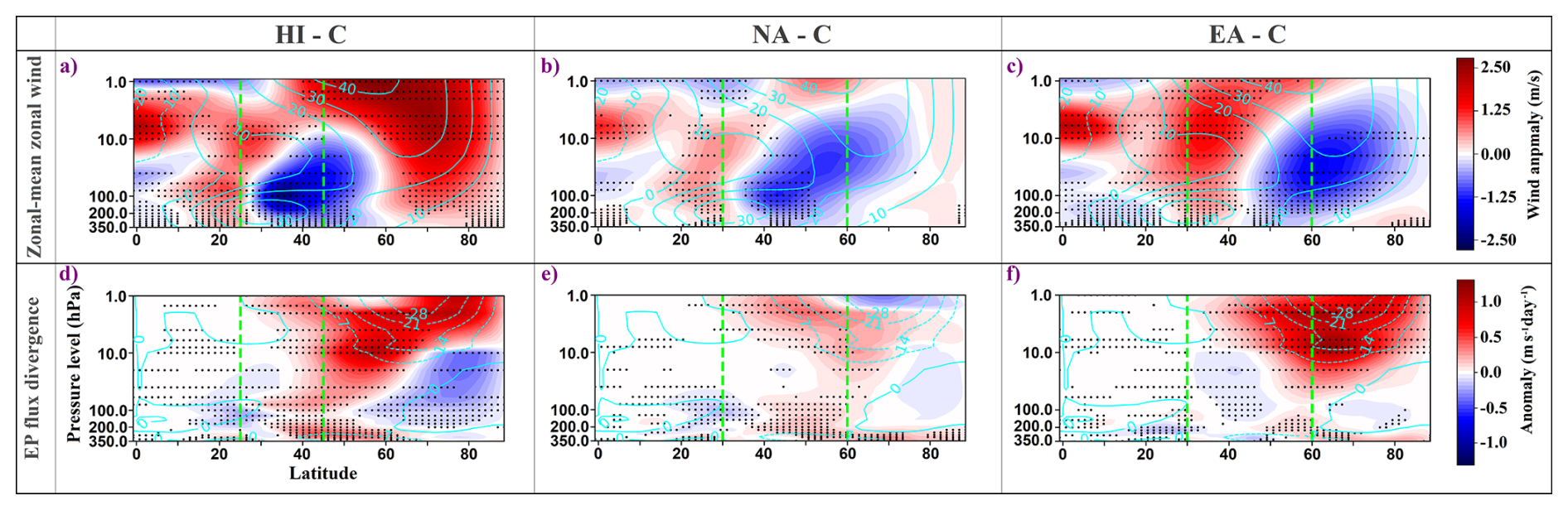
Figure 5 Zonal-mean zonal wind (top row; a–c) and EP flux divergence (bottom row; d–f) anomalies for the HI (left column), NA (middle column), and EA (right column) sensitivity experiments, respectively. Anomalies are computed as the difference between each sensitivity experiment and the control run, based on ensemble means for extended winter (NDJFM). Cyan contours represent the control run climatology of the zonal-mean zonal wind (m s⁻¹; top row) and EP flux divergence (m s⁻¹ d⁻¹; bottom row), with solid lines representing positive values and dashed lines showing negative values. Dotted areas indicate regions where anomalies are consistent across ensemble members. Green dashed lines mark the latitudinal extent of the imposed forcing in each experiment. Adapted from Mehrdad et al. (2025a).

3.2 SPV class centers

Figure 6 displays the resulting GPH class centres, derived from all the control and sensitivity experiments, with red contours overlaid (C2–C10) showing SPV boundaries that were reconstructed from the mean feature vector of each cluster. These reconstructed boundaries closely follow the mean 10 hPa GPH field for their respective clusters, underscoring the physical consistency of the classification.

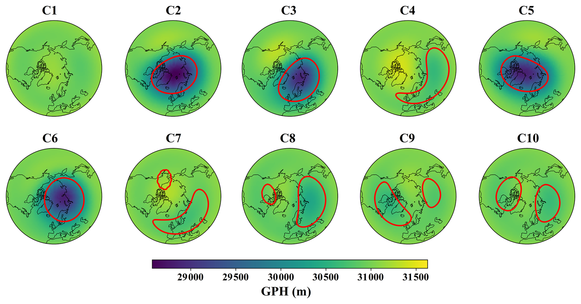
Figure 6 Composite 10 hPa GPH fields for SPV classes C1–C10 during the extended winter season (NDJFM), obtained by averaging all daily GPH fields assigned to each cluster across all experiments. Red contours in clusters C2–C10 represent reconstructed vortex boundaries derived from the average feature vectors of all SPV boundary objects associated with each cluster. Cluster C1, which includes unstable or undefined SPV configurations, does not include a reconstructed boundary.

Class C1 corresponds to an unstable or dissipated vortex, characterized by elevated GPH values near the pole. C2 depicts a centered, deep vortex with slightly elevated GPH over the Pacific sector. C3 shows a moderately displaced vortex shifted toward Eurasia, stretched across the north Eurasia coasts with elevated GPH over North-Western America. C4 represents a highly displaced vortex associated with displaced SSW events, primarily shifted toward the Eurasian continent. The dendrogram in Fig. 2 reveals that C2, C3, and C4 are in the same branch, which reflects their similar structural characteristics and the evolution of high-GPH regions from the Pacific in C2 to North America and the central Arctic in C3 and C4 that are closely related in the dendrogram.

C5 shows a deep vortex cluster that stretches from North America to the north of Eurasia. C6 also illustrates a deep vortex cluster that extends across the north Eurasian coasts with a more circular shape. C7 and C8 are split-vortex cases, with the dominant lobe over Eurasia and a smaller one over North America; these two are also closely linked in the dendrogram. In C9, the North American lobe is dominant and extends over the Atlantic, while in C10, both lobes are of comparable size. These latter two classes also form a distinct branch in the dendrogram. Overall, the correspondence between the class centres and the hierarchical dendrogram confirms the robustness of the shape-based SPV classification. A detailed overview of the corresponding climatological PW1 and PW2 amplitudes for each SPV class is presented in Appendix D (see Fig. D1).

Figure 7 presents the extended winter occurrence frequencies, calculated as the percentage of days each cluster occurs relative to the total days in the period across all ensembles, of SPV clusters C1–C10 (as shown in Fig. 6) in the control run on top of each panel, along with the occurrence differences in the three sensitivity experiments (EA–C, NA–C, HI–C) as color bars. The occurrence frequencies are computed using all ensemble members, with standard deviations calculated across the respective six ensembles. For the control run, these standard deviations are reported as ± values, while in the sensitivity experiments, they are shown as error bars on the bars representing mean differences. Hatching indicates that the sign of the anomaly is consistent across at least five out of six ensemble members.

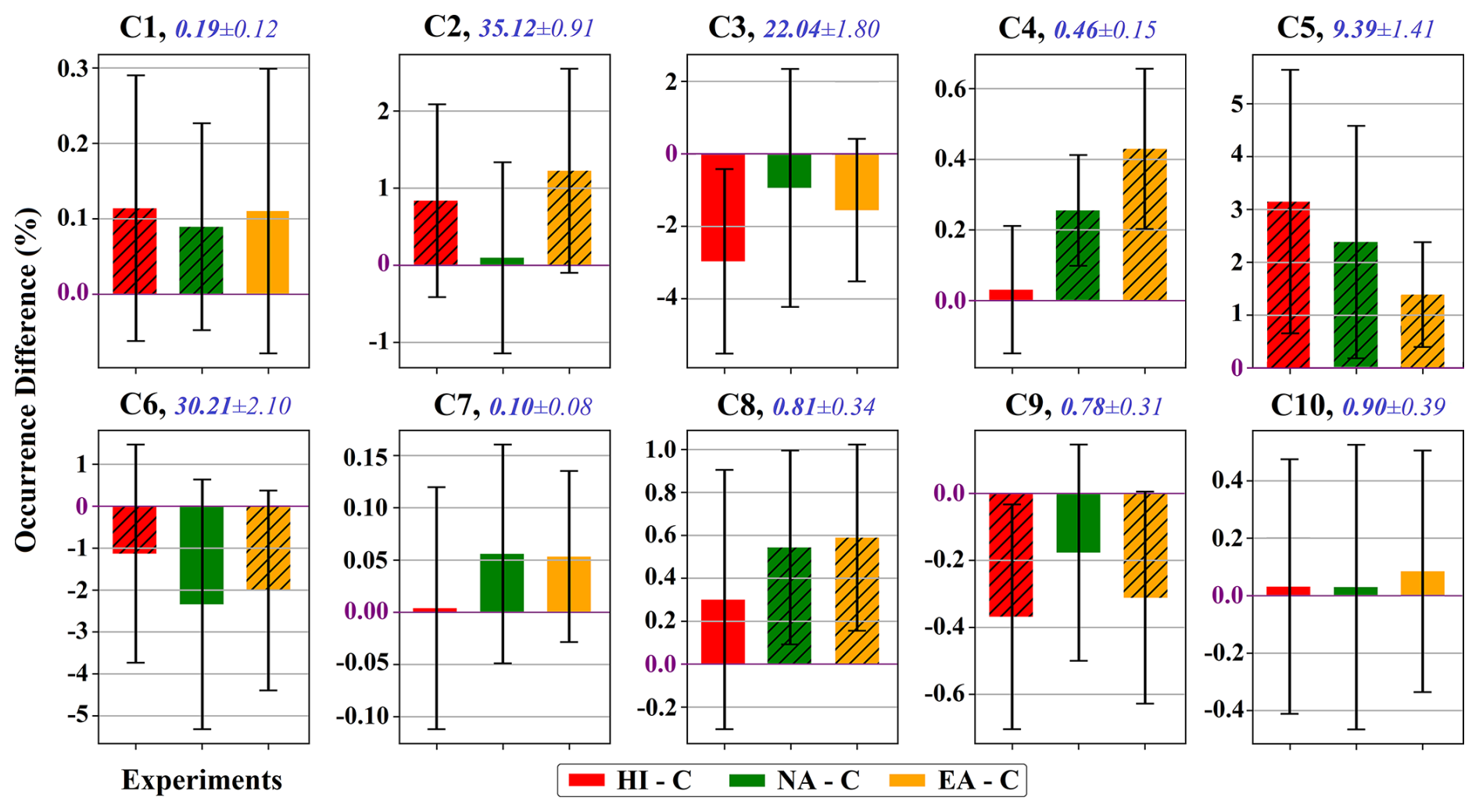
Figure 7 Occurrence frequency differences (%) between each experiment and the control run for SPV clusters C1–C10 during the extended winter season (NDJFM). Differences are calculated as the mean difference across ensemble members for each experiment (HI–C: red, NA–C: green, EA–C: orange). Error bars represent the standard deviation of the differences across the six ensemble members. The horizontal purple line at 0 % marks the control run baseline. Bars are hatched when the sign of the difference is consistent with the ensemble-mean value in at least five out of six ensemble members. The extended winter occurrence frequency (%) of each cluster in the control run is shown above each panel in blue, with ± values indicating the standard deviation across control ensemble members. Note the different y axis scaling for each cluster.

Among the clusters, C2 has the highest mean occurrence in the control run (35.12 % ± 0.91 %), followed by C6 (30.21 % ± 2.10 %), C3 (22.04 % ± 1.80 %), and C5 (9.39 % ± 1.41 %). While the absolute frequencies vary under different experiments, these four clusters remain the most frequent across all experiments. Among the less frequent clusters, C4 represents displaced SSW states, whereas C7-C10 correspond to split SSWs. C1, in contrast, does not exhibit a well-defined vortex structure and represents unstable vortex configurations.

The HI experiment shows a consistent increase in the frequency of C1, C2, and C5, and a consistent decrease in C6 and C9. NA shows consistent increases in C1, C4, C5, and C8. The EA experiment shows consistent increases in C2, C4, C5, and C8, and consistent decreases in C6 and C9. Cluster C3 exhibits a mean decrease in all experiments but does not show ensemble consistency in any case.

3.3 Himalayas (HI)

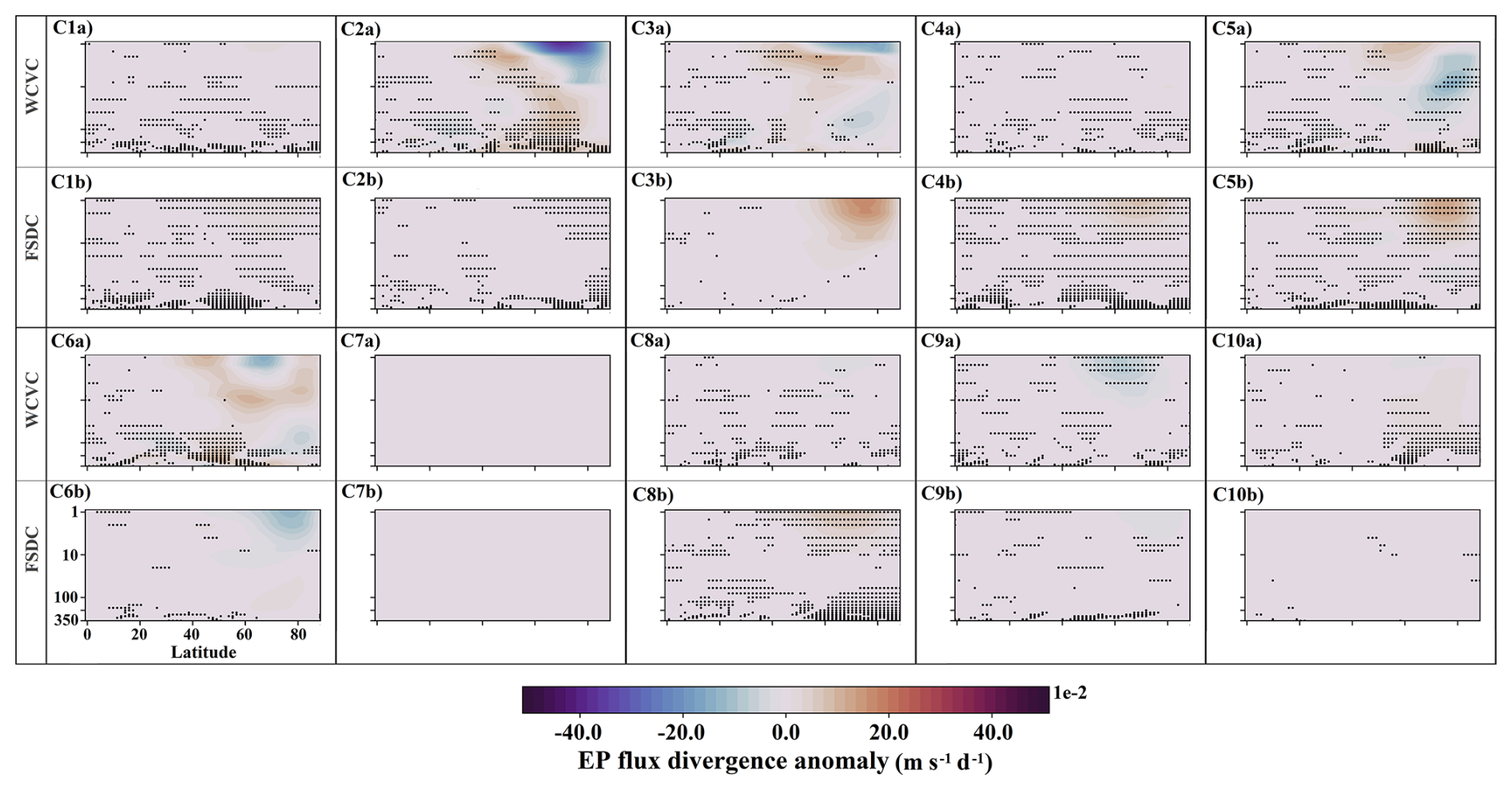
Figure 8 shows the contributions of individual SPV clusters to the 10 hPa GPH anomaly in the HI experiment (see Fig. 3b). Each cluster contributes through WCVC (changes in mean structure) and FSDC (changes in occurrence frequency). The clusters do not contribute equally; their impacts vary in spatial pattern, magnitude, and consistency. Dominant contributions come from frequent clusters C2, C3, C5, and C6. The WCVC of C6 deepens the vortex over the central Arctic (panel C6a), indicating that when C6 occurs in the HI experiment, it consistently exhibits a stronger vortex than in the control run. In contrast, the FSDC of C5 weakens the PW1 structure (panel C5b), reflecting the impact of its consistently increased frequency in HI (see Fig. 7). The WCVC components of C2 and C3 contribute with patterns opposing the PW1 climatology, thereby reducing PW1 amplitude (panels C2a and C3a); C2, in particular, consistently lowers GPH over the Pacific sector. Other clusters play smaller roles, for example, the reduced frequency of C9 yields modest but consistent negative GPH anomalies at high latitudes via its FSDC component (panel C9b).

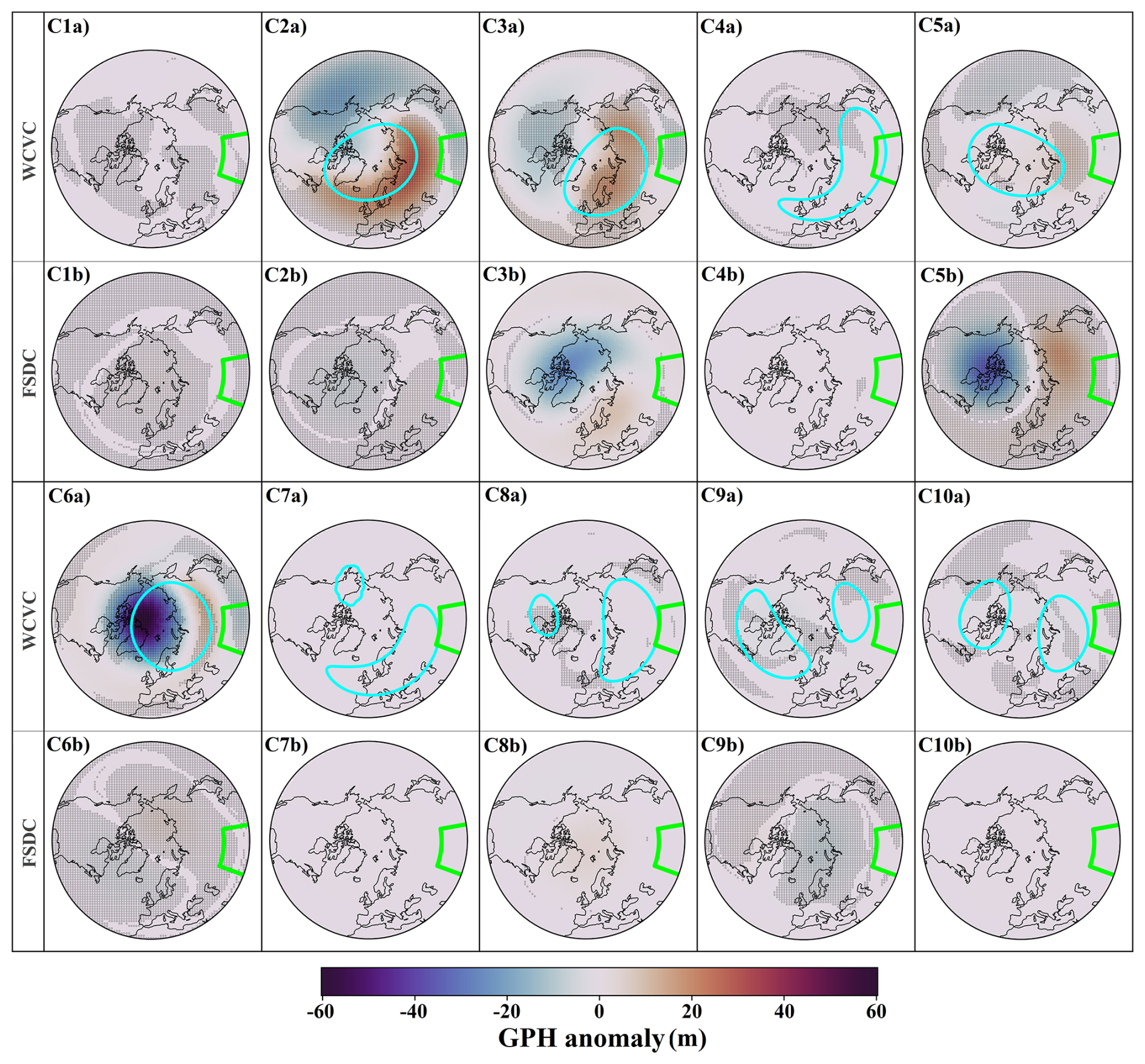
Figure 8 Class contributions to the 10 hPa GPH anomaly for the HI experiment. Each panel (e.g., C1a/C1b to C10a/C10b) corresponds to one SPV class. For each class, the top sub-panel (a) shows the Within-Cluster Variability Contribution (WCVC), and the bottom sub-panel (b) shows the Frequency-weighted Seasonal Deviation Contribution (FSDC). For each SPV cluster, the mean boundaries shown in Fig. 6 are also overlaid with cyan contours in the WCVC sub-panels. Dotted areas indicate regions where the class contribution is consistent across at least five out of six ensemble members. The green outline marks the forced region in the HI experiment.

Figure 9 shows the class contributions to the zonal-mean zonal wind anomaly, as shown in Fig. 5a. The WCVC components of C2, C3, C5, and C6 weaken the midlatitude westerlies from the upper troposphere into the middle stratosphere, reflecting direct forcing effects. C6 primarily strengthens the high-latitude westerlies through its WCVC component (panel C6a). The increased frequency of C5 and the decreased frequency of C9 (see Fig. 7) lead to modest but consistent high-latitude westerly enhancements via their FSDC components (panels C5b and C9b). C3’s FSDC also contributes to upper-stratospheric westerly enhancement, though inconsistently, reflecting the similarly inconsistent reduction in its occurrence change. The WCVC components of C2 and C3 resemble the overall HI wind anomaly pattern.

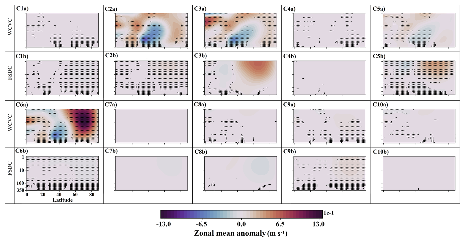
Figure 9 Similar to Fig. 8 but computed for zonal-mean zonal wind. The vertical levels in latitude-height plots are represented in hPa.

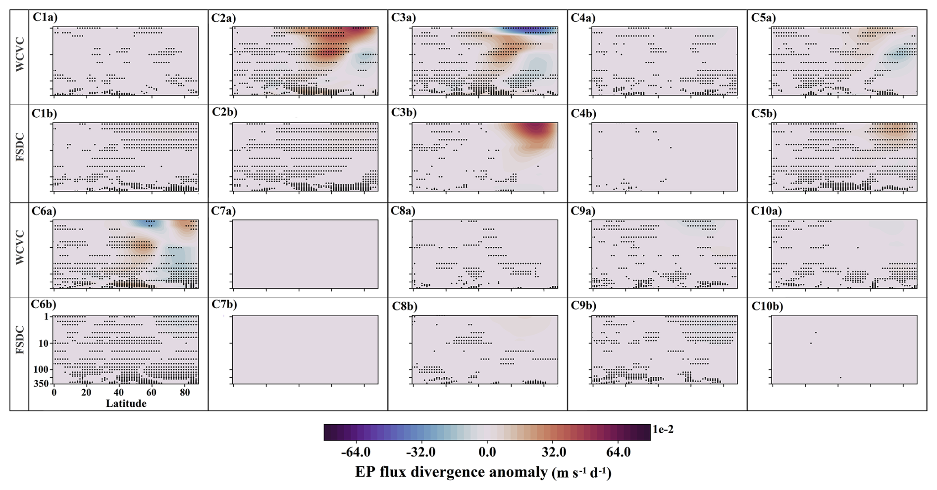
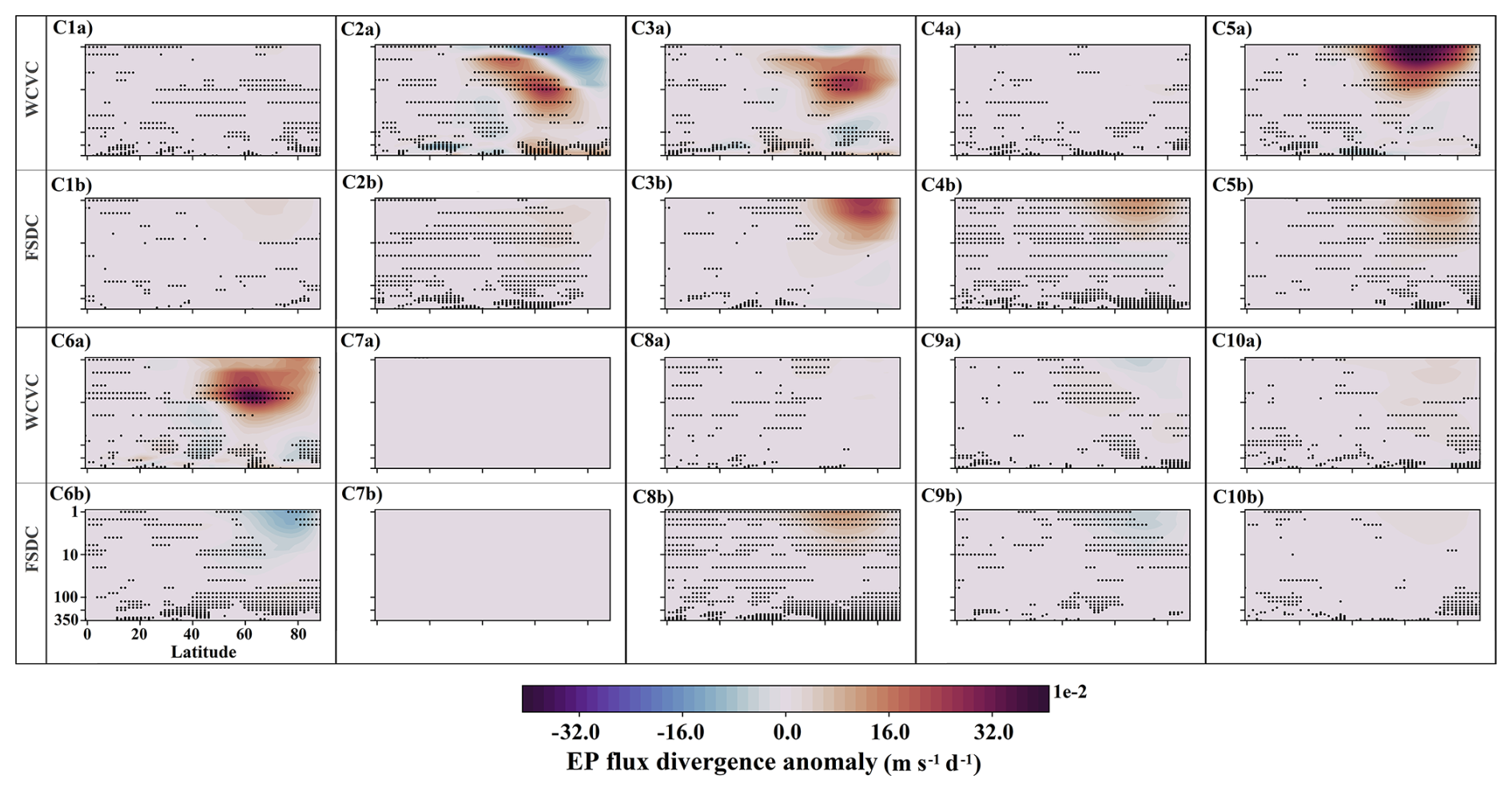
Figure 10 shows the class contributions to EP flux divergence anomalies, as presented in Fig. 5d. The WCVC component of C2 produces positive anomalies in the midlatitude middle and upper stratosphere, indicating reduced wave drag (panel C2a). C3 and C6 contribute modestly to similar positive anomalies through their WCVC components, while also enhancing wave drag in the high-latitude lower and middle stratosphere (panels C3a and C6a). The increased frequency of C5 (see Fig. 7) yields a consistent positive contribution in the high-latitude upper stratosphere via its FSDC component (panel C5b). C3's FSDC also contributes positively in this region, although inconsistently across ensemble members.

Figure 10 Similar to Fig. 9 but computed for EP flux divergence.

3.4 Northwest America (NA)

Figure 11 shows the class contributions to the 10 hPa GPH anomaly in the NA experiment (see Fig. 3c). In general, both the class contributions and the resulting anomaly patterns are less consistent than in the HI and EA (see below) experiments. The consistent increase in the frequency of C5 in the NA experiment (see Fig. 7) results in a consistent contribution through its FSDC component, which resembles a weakening of the climatological PW1 structure (panel C5b). The WCVC of C2 consistently lowers GPH over the Pacific sector (panel C2a) but also produces an inconsistent positive anomaly over the Arctic. C6 contributes a consistent positive anomaly over northeastern Asia through its WCVC component (panel C6a). C4 and C8, whose frequencies increase consistently in the NA experiment, provide modest but consistent positive contributions over the Arctic via their FSDC components (panels C4b and C8b).

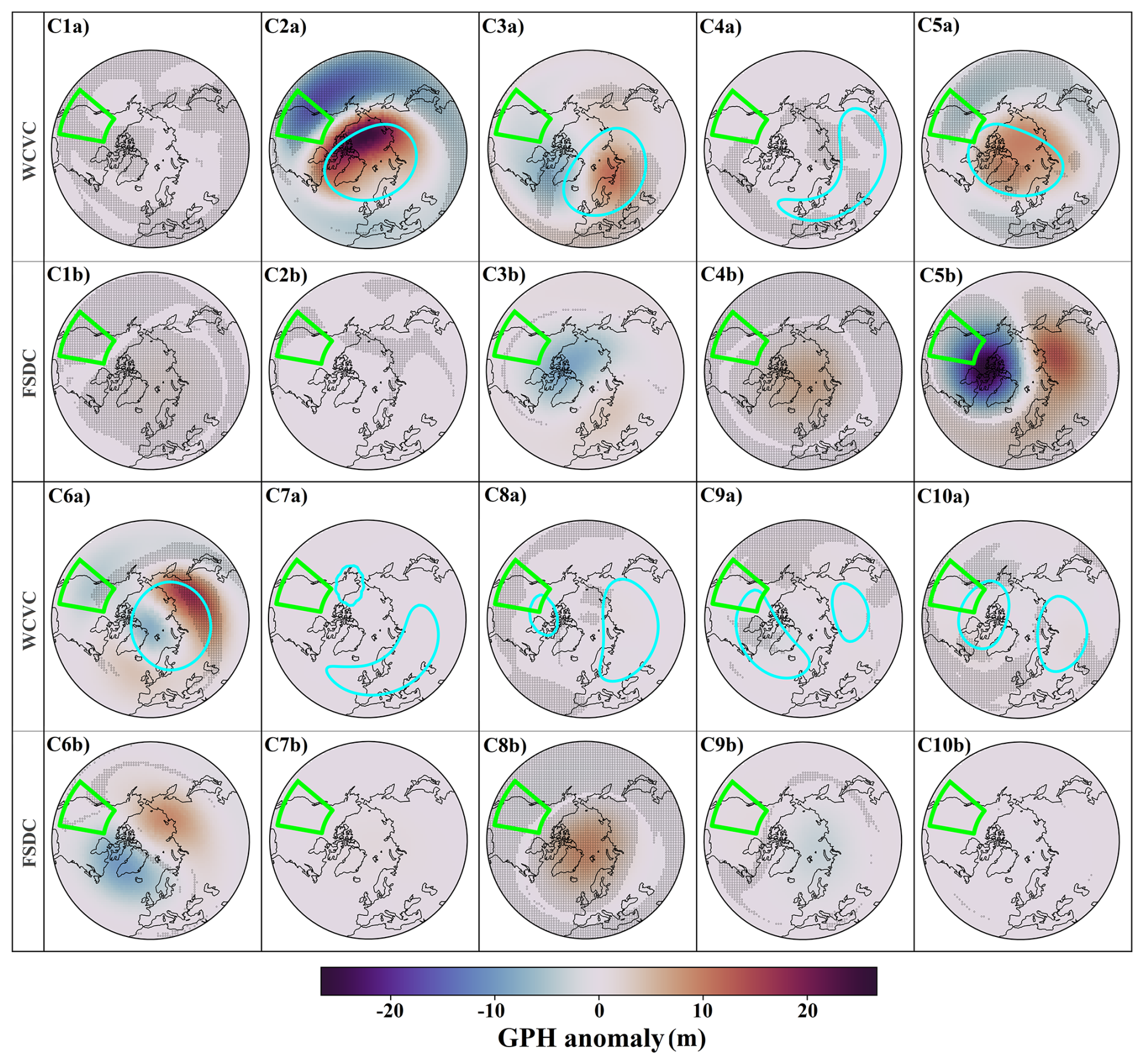
Figure 11 Similar to Fig. 8 but for the NA experiment.

Figure 12 shows the class contributions to the zonal-mean zonal wind anomaly in the NA experiment (see Fig. 5b). The direct weakening effects of zonal-mean zonal wind westerlies associated with the imposed forcing are evident in the WCVC components of C2, C3, C5, and C6. The increased frequency of C5 (see Fig. 7) produces a consistent strengthening of the high-latitude upper-stratospheric westerlies via its FSDC component (panel C5b). Similarly, the increased frequencies of C4 and C8 yield a modest but consistent weakening of the high-latitude stratospheric westerlies through their FSDC components (panels C4b and C8b). The WCVC of C2 produces a strong but largely inconsistent weakening across the mid- and high-latitude stratosphere (panel C2a), while C6’s WCVC strengthens the upper-stratospheric flow at high latitudes, also inconsistently (panel C6a).

Figure 12 Similar to Fig. 9 but for the NA experiment.

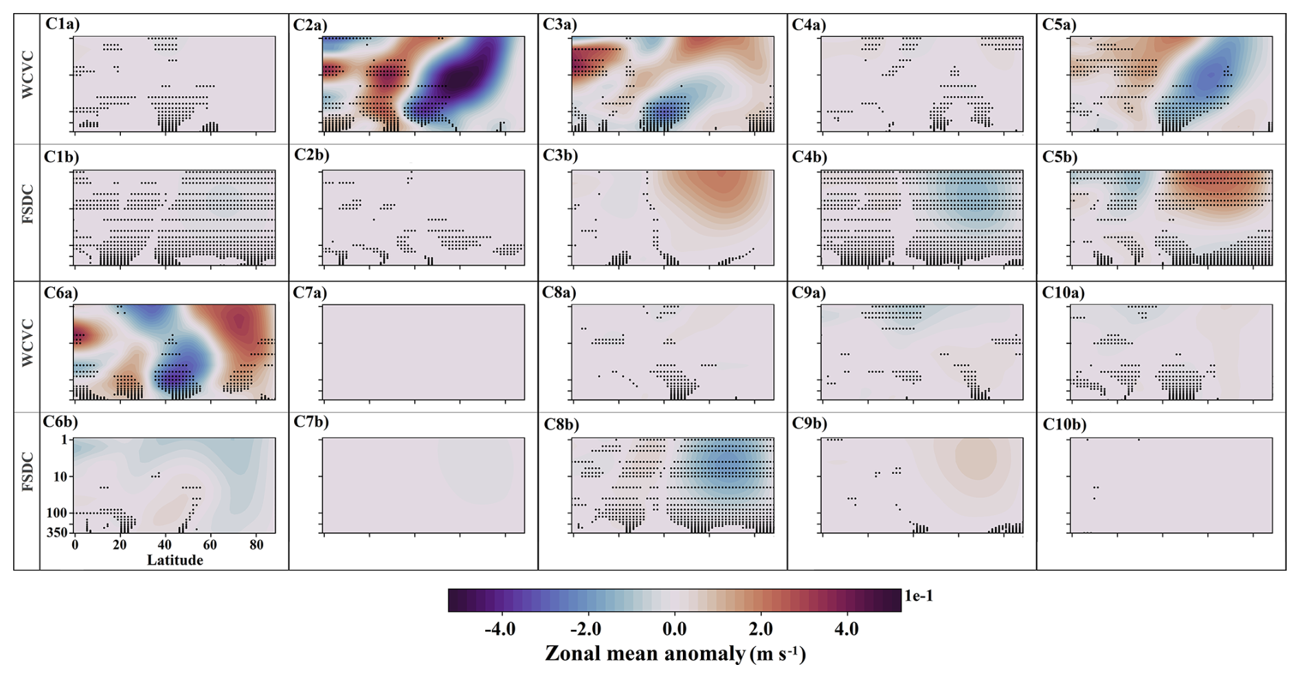
Figure 13 shows the class contributions to the EP flux divergence anomaly in the NA experiment (see Fig. 5e). The increased frequencies of C4, C5, and C8 (see Fig. 7) provide modest but consistent positive contributions in the high-latitude upper stratosphere via their FSDC components (panels C4b, C5b, and C8b). The WCVC component of C2 contributes consistently to positive EP flux divergence anomalies from the high-latitude lower stratosphere into the midlatitude upper stratosphere (panel C2a). Contributions from the other clusters are generally not consistent across ensemble members.

Figure 13 Similar to Fig. 10 but for the NA experiment.

3.5 East Asia (EA)

Figure 14 shows the class contributions to the 10 hPa GPH anomaly in the EA experiment (see Fig. 3d). Overall, the cluster contributions in EA are similar to those in NA, but they are more consistent across ensemble members. The increased frequency of C5 in the EA experiment (see Fig. 7) produces an FSDC contribution that weakens the climatological PW1 pattern (panel C5b). The reduced frequency of C6 yields a wave-1-like response that is slightly shifted relative to the climatology (panel C6b). The increased occurrence of C4 and C8, clusters associated with SSWs, leads to consistent positive GPH anomalies at high latitudes through their FSDC components (panels C4b and C8b). The decreased frequency of C9 and increased frequency of C2 both contribute to a moderate but consistent negative high-latitude GPH anomaly (panels C9b and C2b). The WCVC components of C2, C3, C5, and C6 also contribute notably. C2 exhibits a dipole pattern, with a negative anomaly over the Pacific sector and a positive anomaly at high latitudes (panel C2a). C3 shows a moderate weakening of the PW1 structure (panel C3a). C6 is mostly negative overall, with a localized positive anomaly over northeastern Asia (panel C6a).

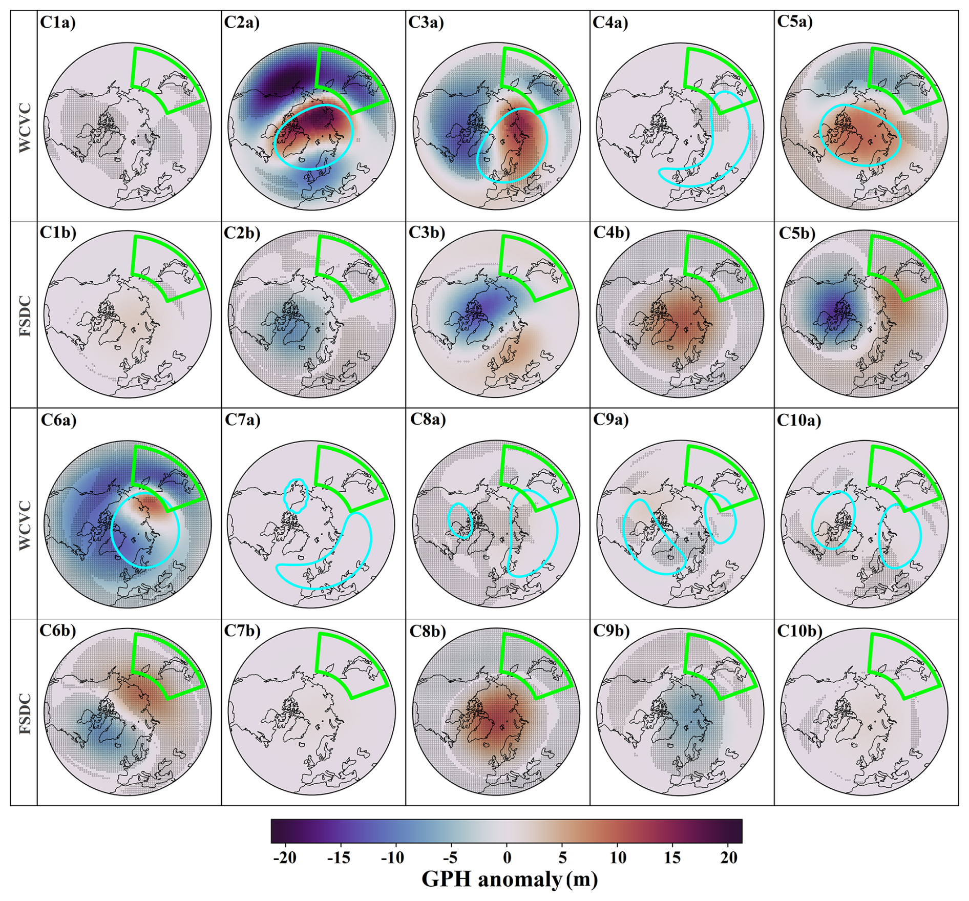
Figure 14 Similar to Fig. 8 but for the EA experiment.

Figure 15 shows the class contributions to the zonal-mean zonal wind anomaly in the EA experiment (see Fig. 5c). The WCVC component of C2 is the primary and most consistent contributor, weakening the high-latitude westerlies and strengthening the midlatitude westerlies (panel C2a). C5 and C6 show similar patterns through their WCVC components, but with more moderate amplitude and less consistency (panels C5a and C6a). The increased occurrence of C4 and C8 in EA (see Fig. 7) leads to a modest but consistent weakening of the high-latitude westerlies via their FSDC components (panels C4b and C8b). By contrast, the increased occurrence of C2 and C5, together with the decreased occurrence of C9, enhances the high-latitude westerlies through their FSDC components (panels C2b, C5b, and C9b), partially compensating the net high-latitude weakening seen in the total anomaly.

Figure 15 Similar to Fig. 9 but for the EA experiment.

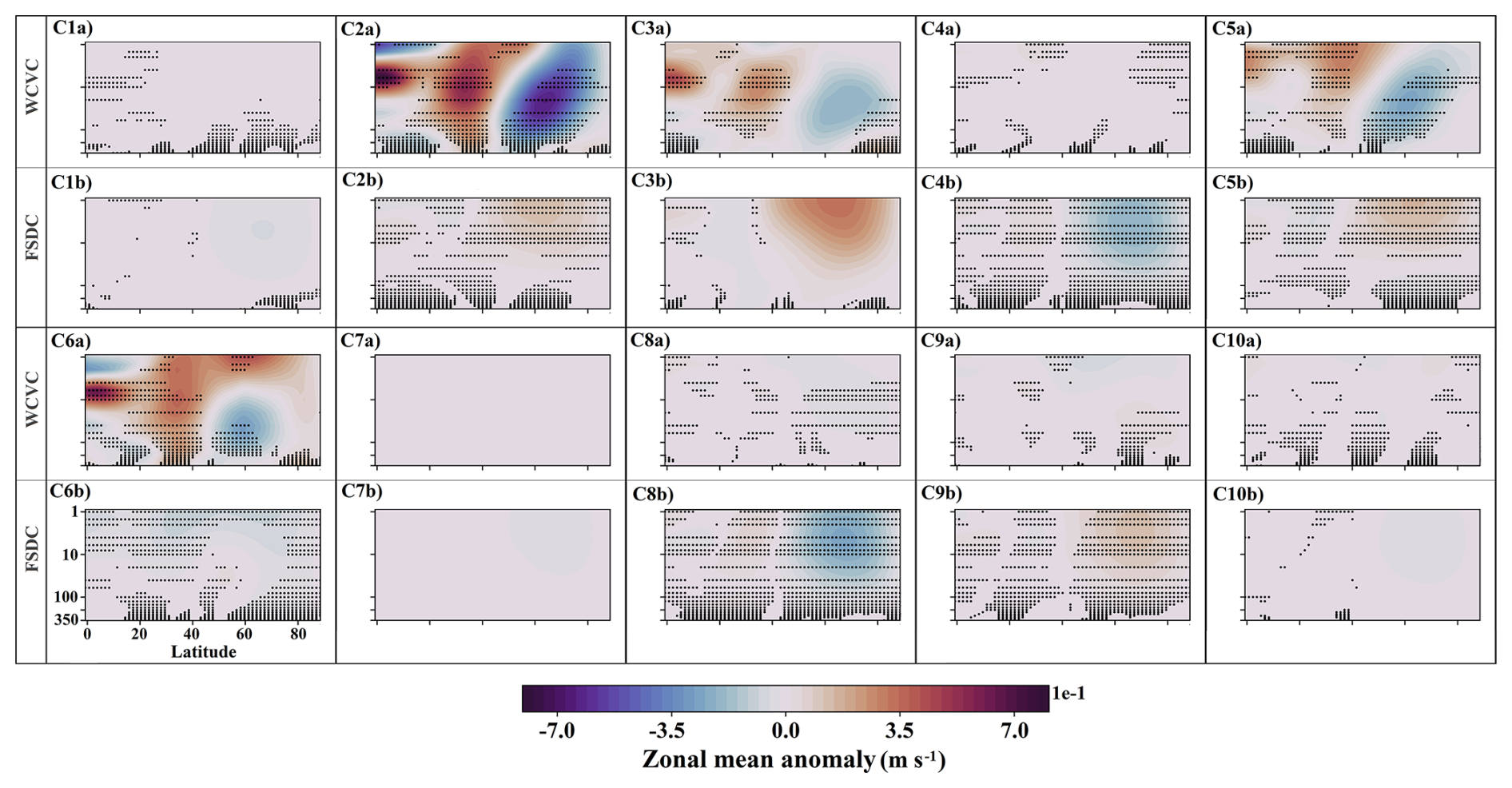
Figure 16 shows the class contributions to the EP flux divergence anomaly in the EA experiment (see Fig. 5f). The increased occurrence frequencies of C2, C4, C5, and C8 in EA (see Fig. 7) produce modest but consistent positive anomalies in the high-latitude upper stratosphere via their FSDC components (panels C2b, C4b, C5b, and C8b), whereas the decreased occurrence of C9 contributes a modest negative anomaly through FSDC (panel C9b). The WCVC component of C5 is the primary contributor to the positive EP flux divergence anomalies in the high-latitude upper stratosphere (panel C5a). In addition, the WCVC components of C6, C3, and C2, listed in order of decreasing strength, also contribute consistently to positive anomalies in the middle and upper stratosphere (panels C6a, C3a, and C2a).

Figure 16 Similar to Fig. 10 but for the EA experiment.

4 Discussion and conclusions

4.1 Common response to localized GW forcing

This study provides new insights into the response of the SPV to GW forcing in Northern Hemisphere stratospheric hotspots using a novel shape-based clustering approach. The SPV does not respond in a zonally symmetric manner to localized GW forcing in the defined hotspot regions. Across all experiments, regardless of the specific hotspot location, the response consistently features a PW1-like displacement of the vortex core (Fig. 3). This involves a more irregular, ragged edge over northern Eurasia, although the detailed anomaly pattern remains distinct for each case. The dominant dynamical feature underlying these anomalies is the consistent reduction in the amplitude of PW1 across all experiments. This is also evident in the EP flux divergence anomalies (Fig. 5), which show positive EP flux divergence anomalies associated with the PW1 structure in the midlatitude stratosphere (Mehrdad et al., 2025a).

Our results differ in some aspects for the hotspot regions compared with Sacha et al. (2021) and Kuchar et al. (2022). They analyse short-timescale event composites of strong SSO GW drag peaks in a specified-dynamics Canadian Middle Atmosphere Model (CMAM) framework in the lower stratosphere. By contrast, we impose localized enhancements of SSO drag in a free-running UA-ICON ensemble and evaluate NDJFM season-mean responses across 180 simulated years. In this climate-mean framework, the time-integrated effect of many intermittent events, together with the background-state adjustments induced by the forcing, yields a hemispheric reduction of PW1 amplitude and weaker resolved wave drag. Differences thus arise from (i) timescale and averaging (event composites vs. season-mean) and (ii) model configuration and the associated background-state evolution.

These anomalies manifest as negative GPH anomalies within the forced region and positive anomalies northward of it (Fig. 3). A plausible explanation is that enhanced GW drag near the forced region disrupts the SPV edge through increased small-scale wave breaking and secondary instabilities, thereby promoting geometry-specific PV redistribution rather than a uniform vortex response (Coy et al., 2024). This mixing across the vortex boundary locally blurs the typically sharp SPV edge, resulting in the observed pattern of anomalies. Specifically, positive GPH anomalies at the SPV periphery often indicate incursions of low-PV, warm high-pressure ridges, while negative anomalies reflect high-PV polar air being displaced equatorward, forming cold low-pressure troughs (Fig. B1). Such patterns are characteristic of surf zone wave activity impinging on the SPV (Waugh, 1997). The HI experiment, which represents the southernmost hotspot region, shows the strongest response, with the positive anomaly band north of the forcing extending only to the northern Eurasian coastline. The latitudinal position of the positive anomaly band in the HI experiment, located well south of the vortex edge over northern Eurasia, effectively sharpens the vortex edge in that sector and further deepens the polar vortex core toward higher latitudes.

4.2 Cluster-based characterization of the response

Examining the forcing effect on the occurrence frequency of the preferred SPV geometry clusters (as detailed in Sect. 3.2; see also Fig. 6) reveals a consistent increase in the occurrence of C5 across all experiments (Fig. 7). Among the single vortex clusters (C2–C6), C5 has the weakest PW1 amplitude except for C4, which represents displaced SSW events (Fig. D1, left panel). The PW1 amplitude associated with C5 remains well below the climatological mean, suggesting that its increased occurrence frequency contributes to or favors the reduction in PW1 amplitude observed across all three experiments. This effect is clearly evident in the FSDC components of C5’s contributions to the 10 hPa GPH anomalies, which exhibit a pattern opposite to the PW1 climatology (panel C5b in Figs. 8, 11, and 14). A similar signal is apparent in the EP flux divergence anomalies, with positive anomalies consistent with a weakened PW1 structure (panel C5b in Figs. 10, 13, and 16) Mehrdad et al. (2025a). Although the amplitude of this contribution varies among experiments, it remains a consistent feature. However, it does not represent the dominant driver of the anomalies in any individual case.

C5 is the only cluster that shows a consistent and similar sign change in occurrence frequency across all experiments. There were other clusters where the occurrence frequency change is only consistent in one or two experiments, such as C4 and C8, displaying consistent increases in occurrence frequency only in the EA and NA experiments. These clusters are associated with SSW events, and their increased occurrence contributes to the anomalies by weakening the SPV (see panels C4b and C8b in Figs. 14 and 15 for EA, as well as Figs. 11 and 12 for NA). However, because these clusters have relatively low occurrence frequencies in the climatology, their contributions, though consistent, remains comparatively weak. The robust increased occurrence of these SSW clusters in the EA experiment is consistent with the higher number of SSW events per decade diagnosed for this case (Mehrdad et al., 2025a).

The WCVC component of the class contribution quantifies how the forcing influences the general structure and geometry of a given cluster, but these structural changes are typically small enough that they do not lead to reassignment to a different cluster (Mehrdad et al., 2024). The WCVC contribution is generally stronger in the most frequent clusters (C2, C3, C5, and C6) and often represents the dominant pathway shaping the observed anomalies. However, these structural responses do not always occur consistently across ensemble members, underscoring the role of internal variability, a feature particularly evident in the NA experiment. When consistent, however, the WCVC patterns can be useful for revealing the underlying mechanisms and physically meaningful signals by which localized forcing modifies the SPV.

The consistently increased frequency of C5 across all experiments is not the only factor associated with the reduction in PW1 amplitude observed in all the sensitivity experiments. The WCVC components of the most frequent clusters, such as C2 and C3, also generally exhibit patterns opposing the PW1 climatology, indicating that the forcing tends to modify the prevailing clusters toward configurations with weaker PW1 amplitudes. For example, in the HI experiment, the WCVC component of C3 contributes with a PW1-like pattern; together with C2, these two clusters, both characterized by strong PW1 amplitudes (left panel of Fig. D1), contribute to the anomaly with a pattern opposite to the PW1 climatology. This suggests that the forcing acts to weaken the PW1 amplitude even in clusters that typically exhibit strong PW1 activity.

The WCVC components of C2, C3, and C6 consistently generate positive GPH anomalies north of the forced region and negative anomalies within it. This pattern aligns zonally along the SPV boundaries, which correspond to the GPH isolines representing each cluster’s mean circulation, highlighting how the forcing interacts with the geometry of the SPV. The resulting positive anomaly patches reflect localized SPV edge mixing driven by the forcing and tend to follow the mean circulation (i.e., along the geostrophic wind direction implied by the mean GPH isolines) associated with each cluster, consistent with edge-focused wave breaking and secondary instabilities acting along the vortex boundary (Coy et al., 2024). Notably, for C6, this interaction strengthens the SPV edge by producing a narrow band of higher GPH north of the forced region. This demonstrates how the relative position and geometry of the SPV relative to the hotspot can determine whether the hotspot forcing leads to mixing and weakening or, conversely, to intensification of the vortex structure, indicating a shape-related, geometry-dependent stratospheric adjustment.

4.3 Experiment-specific characteristics

The deceleration of the zonal-mean zonal wind near the forcing region in HI is evident in the WCVC components of the most frequent clusters (Fig. 9), indicating the direct and consistent role of the imposed forcing in shaping these contributions. The WCVC component of C6 emerges as the main contributor to the zonal wind acceleration over the polar regions, consistent with its role in deepening the SPV core. Comparing the class contribution to the EP flux divergence (Fig. 10) and zonal-mean zonal wind reveals that they do not always align straightforwardly across clusters. For example, in the midlatitude lower and mid-stratosphere, the deceleration of the mean flow is not accompanied by corresponding negative anomalies in EP flux divergence as would typically be expected. This discrepancy suggests that other momentum sources, such as GW drag imposed in the experiment Mehrdad et al. (2025a), play a dominant role in this region (see Fig. A2). Similar inconsistencies are apparent in the C6 WCVC component, where positive anomalies in EP flux divergence do not coincide with stronger westerlies (see panel C6a in Figs. 9 and 10). Overall, such differences arise because the class contribution framework captures the simultaneous response but does not account for the delayed adjustments that are typical of wave–mean flow interactions.

For the NA experiment, the most consistent contributions arise from the FSDC components of clusters C4, C5, and C8, which reflect the consistent increase in their occurrence frequencies. In contrast, other class contributions, while locally strong, tend to be less consistent. The WCVC components of C2, C3, and C6, for example, display localized patches of positive GPH anomalies in a higher-latitude band north of the forced region, extending along the SPV boundary in a manner similar to the HI experiment (Fig. 11), but with only partial consistency. Notably, the WCVC contribution of C2 is particularly strong and extends into the polar region, but it is consistent only in a relatively small area northeast of North America. This pattern is linked to the C2 WCVC’s associated deceleration of the zonal-mean zonal wind in the mid- and high-latitude stratosphere (panel C2a in Fig. 12), which also shows patchy consistency, especially at higher latitudes. Overall, this highlights how internal variability in the NA experiment tends to obscure clear, spatially coherent responses to the imposed forcing, in contrast to the more robust signals evident in the HI experiment.

In the EA experiment, the class contributions are generally similar to those in the NA experiment but exhibit more spatially consistent signals. This similarity likely stems from the more northward placement of the NA and EA hotspots compared to the HI hotspot, which might influence the location and magnitude of the SPV response. The greater consistency observed in the EA experiment compared to NA can also be related to the relative phase alignment of the hotspot region with the stationary PW1 pattern (Mehrdad et al., 2025a). Across all experiments, a common feature is the presence of a positive GPH anomaly north of the forced region, indicative of PV mixing along the SPV edge. Notably, the responses in NA and EA, the two more poleward hotspots, show deeper intrusions of this anomaly into the polar vortex core compared to the HI experiment.

4.4 Model limitations and implications

Like in any sensitivity study, the results may be influenced by inherent biases in the underlying model. In this study, UA-ICON, in its default configuration, exhibits a SSO-induced GW drag maximum in the mid-latitude lower stratosphere (see Fig. A2), corresponding to the so-called valve layer (Kruse et al., 2016). This maximum occurs slightly lower than the multi-model mean in the Coupled Model Intercomparison Project Phase 6 (CMIP6) Atmospheric Model Intercomparison Project (AMIP) simulations (Hájková and Šácha, 2024). A lower placement of this SSO-induced drag peak may influence the interaction between parameterized and resolved waves and, consequently, aspects of the simulated stratospheric dynamics. A quantitative assessment of the sensitivity of these interactions to the vertical placement of the valve-layer maximum would require dedicated experiments, which lie beyond the scope of this work.

Overall, localized GW drag exerts a decisive yet geometry-sensitive influence on SPV variability. The shape-based clustering and class contribution framework developed in this study help reveal robust and spatially coherent responses to localized forcing that might otherwise be obscured by internal variability within the full ensemble. While the current analysis is limited to present-day climatological conditions, extending this morphology-based approach to transient climate scenarios and observational reanalyses would further test its utility. Such applications could improve our understanding of the mechanisms governing SPV variability and offer new opportunities for enhancing subseasonal prediction.

Appendix A: SSO-induced zonal drag

Figure A1 shows the climatology and anomalies of the SSO-induced zonal (U) tendency, scaled by layer pressure and averaged over the stratosphere during the extended winter season (November through March, NDJFM). The left panel presents the climatology from the control run (C), while the three right panels display anomalies for the HI, NA, and EA sensitivity experiments relative to the control. As expected, the control run exhibits stronger SSO-induced drag over major topographic regions, and enhanced zonal drag appears within the prescribed hotspot regions (outlined in green), indicating localized amplification of the SSO forcing.

Figure A2 summarizes how the SSO parameterization projects onto the zonal-mean circulation during NDJFM. Panel a shows the extended-winter climatology of the SSO-induced zonal-wind tendency in the control run (C). The SSO scheme imparts easterly drag (negative values) with two notable features: a broad upper-stratosphere/lower-mesosphere maximum at midlatitudes and a secondary maximum in the lower stratosphere associated with the valve layer (Kruse et al., 2016). The latter is located on the upper flank of the zonal-mean upper-troposphere–lower-stratosphere (UTLS) jet. In UA-ICON, this lower-stratospheric peak appears slightly lower in altitude than in the CMIP6 AMIP multi-model mean (Hájková and Šácha, 2024), which may influence the interaction between parameterized and resolved waves.

Panels (b)–(d) show anomalies relative to the control (HI–C, NA–C, EA–C, respectively). Each hotspot intensifies easterly tendencies primarily within its forced latitude band (green dashed lines), but the vertical structure differs by regions. In HI, the largest anomalies occur in the lower stratosphere with a coherent upward extension (Fig. A2b). NA exhibits a similar lower-stratospheric strengthening that is more confined in height and accompanied by upper-level westerly anomalies (Fig. A2c). EA shows a broader, more vertically extended enhancement with less emphasis on a distinct lower-stratospheric peak (Fig. A2d). These differences reflect variations in SSO wave generation within the scheme and differences in the background flow for each hotspot. For additional diagnostics, see Mehrdad et al. (2025a).

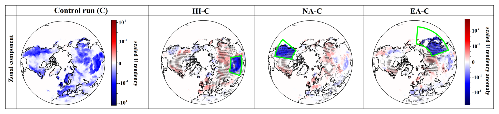
Figure A1 Spatial distribution of the SSO-induced zonal (U) tendency scaled by layer pressure and averaged over the vertical extent from 200 to 1 hPa during the extended winter season (NDJFM). The results are based on the ensemble mean for (left) the climatology of the control run (C) and (right) the sensitivity experiments (HI–C, NA–C, and EA–C, respectively) relative to the control run. Dotted areas indicate regions where the anomaly is considered consistent, meaning that at least five out of six ensemble members exhibit the same anomaly sign as the ensemble-mean anomaly. The forced regions in each experiment are outlined in green. The color bars on the right represent values on a logarithmic scale. This figure is adapted from Mehrdad et al. (2025a).

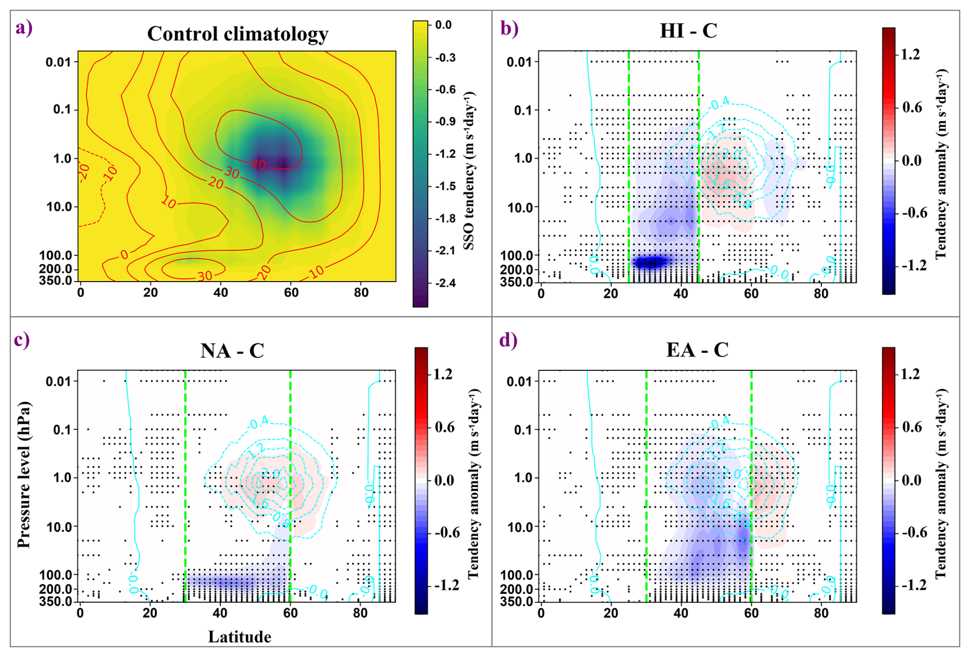
Figure A2 Zonal-mean SSO-induced zonal wind (U) tendency during extended winter (NDJFM). (a) Control climatology (C). (b–d) Tendency anomalies relative to the control for the HI–C, NA–C, and EA–C experiments, respectively (negative values indicate easterly anomalies). Green dashed lines indicate the forced latitude band for each hotspot. Stippling denotes regions where anomalies are consistent across ensemble members. Red contours in (a) show the zonal-mean zonal wind climatology (m s⁻¹), and thin cyan contours in (b)–(d) repeat the control tendency climatology from (a) color shading. Adapted from Mehrdad et al. (2025a).

Appendix B: Potential vorticity (PV)

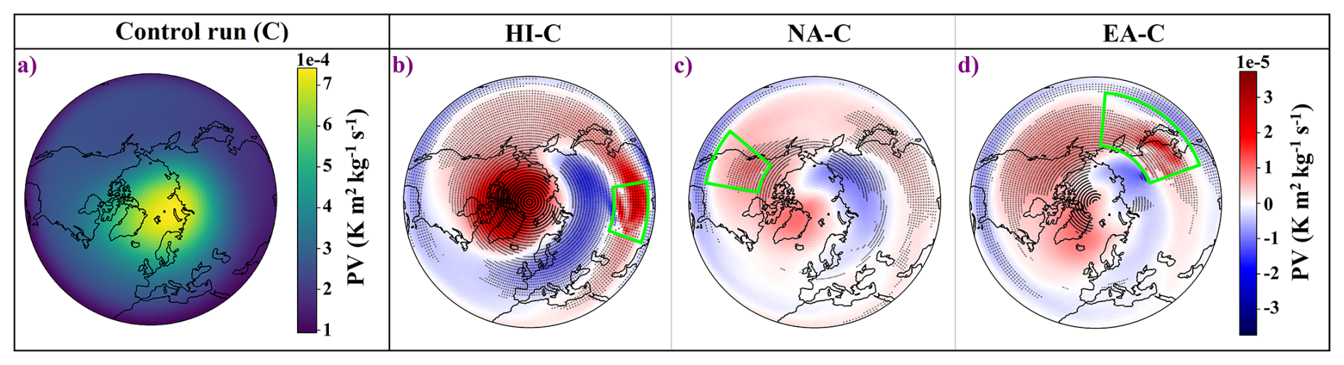
Figure B1 Same as Fig. 3, but for PV on the 850 K isentropic surface. Panel (a) shows the PV climatology from the control run. Panels (b)–(d) display PV anomalies for the HI, NA, and EA simulations, respectively, relative to the control run. Dotted areas indicate regions where anomalies are consistent across at least five of six ensemble members. The forced regions are outlined in green.

Figure B1a shows the climatology of PV on the 850 K isentropic surface, which approximately corresponds to the 10 hPa pressure level, for the control simulation. Figure B1b–d display the corresponding PV anomalies for the HI, NA, and EA experiments. Both the climatological structure and anomaly patterns closely resemble those observed in the 10 hPa GPH fields presented in Fig. 3. As expected, the PV fields exhibit an inverse relationship with the GPH fields; that is, regions of high PV generally correspond to low GPH.

Appendix C: Climatological zonal-mean circulation

Figure C1 presents the extended winter climatology of zonal-mean zonal wind and EP flux divergence in the stratosphere. The zonal wind shows a strong westerly jet centered around 60° N near 10 hPa, characteristic of the climatological SPV. The EP flux divergence pattern illustrates the typical wave forcing on the mean flow, with wave drag dominant in the high-latitude stratosphere. Both fields exhibit realistic structures consistent with previous studies and reanalysis-based climatologies (Edmon et al., 1980; Randel et al., 2004).

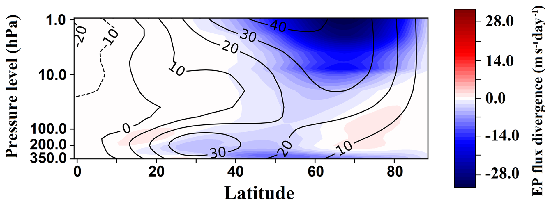
Figure C1 Climatological zonal-mean zonal wind (black contours; in m s⁻¹) and EP flux divergence (color shading) for the control experiment, averaged over the extended winter season (NDJFM), adapted from Mehrdad et al. (2025a).

Appendix D: Climatological latitudinal profiles of PW1 and PW2 amplitudes by SPV class

Figure D1 shows the climatological latitudinal profiles of PW1 and PW2 amplitudes in the control run, along with the corresponding mean amplitudes for each SPV class, calculated across all days labeled to each cluster from all experiments. Cluster C1, representing an unstable vortex, exhibits the lowest amplitudes in both PW1 and PW2. In general, single-vortex classes (C2–C6), with the exception of C4, show higher PW1 amplitudes than the other clusters. Among these, C3 has the strongest PW1 amplitude, while C5 has the weakest one. This is consistent with the vortex morphology. C3 has the most displaced vortex center, whereas C5 shows a more centered structure.

For PW2 (Fig. D1 right panel), C9 has the highest amplitude overall, reflecting its clear two-vortex structure. In the two-vortex structure classes (C7–C10), modest PW1 amplitudes are also present alongside the PW2 activity, indicating a wave-1-like displacement superposed on the PW2 geometry, consistent with the view that SSW morphology is rarely purely binary (Mitchell et al., 2011). Among the single-vortex clusters (C2–C6, excluding C4), C5 exhibits the highest PW2 amplitude, likely associated with its elongated vortex shape. In contrast, C6 and C3 show the lowest PW2 amplitudes, with C6 representing a relatively circular vortex configuration accordingly. Although C3 has low PW2 amplitude, its vortex remains strongly deformed due to dominant PW1 activity, giving it an oval shape.

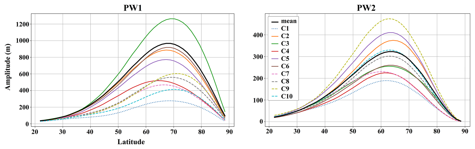
Figure D1 Latitude–amplitude profiles of PW1 (left panel) and PW2 (right panel) in the Northern Hemisphere extratropics for each SPV cluster (C1–C10), shown in different colors. Cluster C1 (unstable vortex) is shown with a dotted line, clusters C2–C6 (single vortex) with solid lines, and clusters C7–C10 (split vortex) with dashed lines. Wave amplitudes are computed from daily 10 hPa GPH fields and averaged over all days classified into each respective cluster during the extended winter season (NDJFM), across all experiments. The black lines in both panels represent the climatological PW1 and PW2 amplitudes calculated from the control experiment. The legend for both panels is shown in the right panel. Note the different scaling in both panels.