NMVOC emission optimization in China through assimilating formaldehyde retrievals from multiple satellite products

Non-methane volatile organic compounds (NMVOCs) are key precursors of ozone and secondary organic aerosols. As one of the world’s largest NMVOC emitters, accurate emission inventories are essential for understanding and mitigating air pollution in China. Commonly-used inventories (e.g., MEIC) are largely based on bottom-up methods, which often fail to capture the spatiotemporal variability of NMVOC emissions, resulting in significant model-observation mismatches. This study evaluates the shape factor, filtered data volume, and monthly mean biases of OMI, OMPS, and TROPOMI formaldehyde products, with the latest OMPS and TROPOMI retrievals offering substantially higher effective spatiotemporal coverage. Monthly NMVOC emissions over China in 2020 are then optimized by independently assimilating formaldehyde retrievals either from OMPS or from TROPOMI, using a self-developed 4DEnVar assimilation emission inversion system. The OMPS- and TROPOMI-driven assimilation yields consistent seasonal and regional increments in NMVOC emissions in general, but distinctions are also notable. A consistency analysis is introduced to assess the reliability of these two posterior emissions. Highly consistent increments are obtained in the North China Plain (May–June), the Yangtze River Delta and Pearl River Delta (January–March, October–December), and the Sichuan Basin (January, June–December). These adjustments significantly improve surface ozone simulations, with 81.25 % of consistent cases demonstrating reduced biases and an average RMSE reduction of 24.7 %. These findings highlight the effectiveness of OMPS and TROPOMI formaldehyde assimilation, coupled with consistency analysis, in refining NMVOC emission estimates and enhancing ozone simulation accuracy. Similar promising results are achieved in the OMPS/TROPOMI-based NMVOC emission inversion in 2019.

1 Introduction

Non-methane volatile organic compounds (NMVOCs) are significant components of the atmosphere, serving as key precursors to ozone (O₃) and secondary organic aerosols (SOA) (Liu et al., 2017). They engage in numerous photochemical reactions, exerting a considerable influence on atmospheric oxidative capacity and air quality (Zhu et al., 2021). Moreover, NMVOCs such as benzene, trichloroethylene, and chloroform are recognized for their toxicity (Billionnet et al., 2011; Lerner et al., 2012), and prolonged exposure to elevated concentrations can pose significant health risks (He et al., 2015). China has seen a rapid anthropogenic NMVOC emissions increase over the last three decades, gradually becoming one of the important contributors to global NMVOC emissions (Li et al., 2019). Investigating NMVOC dynamics and their emission distributions is critical for addressing air pollution challenges in China (Yuan et al., 2013; Hao and Xie, 2018).

NMVOCs are primarily released through anthropogenic activities, biogenic emissions, and biomass burning processes. Huge efforts have been devoted to constructing inventories recording these emissions in a bottom-up way, such as the global Community Emission Data System (CEDS) (Hoesly et al., 2018), the regional Multi-resolution Emission Inventory for China (MEIC) (Li et al., 2019), and the Model of Emissions of Gases and Aerosols from Nature v2.1 (MEGAN) (Guenther et al., 2012). For biomass burning, widely used inventories include the Global Fire Emissions Database (GFED) (van der Werf et al., 2017) and the Fire INventory from NCAR (FINN) (Wiedinmyer et al., 2011). Coupled with chemical transport models like GEOS-Chem (Ito et al., 2007) and WRF-Chem (Azmi et al., 2022), these inventories are widely used to simulate transport, deposition, and chemical transformations of NMVOCs, supporting air quality assessments and emission control strategies. However, bottom-up estimates remain highly uncertain because both emission factors and activity data vary greatly in space and time and are often poorly constrained (Bo et al., 2008; Sharma et al., 2015). For anthropogenic sources, nationwide uncertainties of ±68 %–78 % have been reported due to variable activity data and emission factors under rapid structural transitions in industry, solvent use, and transportation (Li et al., 2017, 2019). Biogenic emissions are even more uncertain, highly sensitive to land-cover, meteorology, and parameterizations, with Chinese BVOC estimates varying from 10 to 58.9 Tg C yr⁻¹ (Li et al., 2020; Wang et al., 2021; Pei et al., 2025). Biomass burning emissions also show large discrepancies across inventories (e.g., GFED, FINN, GFAS) (Kaiser et al., 2012), largely driven by uncertainties in burned area, fuel loading, and emission factors (He et al., 2011; Hua et al., 2024). In addition, strict air pollution controls implemented in recent years targeting industry, residential use, and transportation have significantly altered emission patterns (Wu et al., 2016; Li et al., 2017; Zheng et al., 2018). Consequently, bottom-up inventories carry substantial uncertainties (Li et al., 2014; Qiu et al., 2014). For example, estimates of China’s total NMVOC emissions for 2012 range between 18 and 27 Tg depending on the inventory used (Kurokawa et al., 2013; Wu et al., 2016; Stavrakou et al., 2017), posing major challenges for accurately assessing the role of NMVOCs in air quality and climate (Han et al., 2013; Wang et al., 2014).

There are numerous well-established techniques for measuring the concentrations of various volatile organic compounds in the atmosphere. These include gas chromatography, mass spectrometry, Fourier transform infrared spectroscopy, and non-dispersive infrared analysis. While these methods are highly effective for meeting the requirements of experimental studies and real-time monitoring, their complexity and the associated high labor costs pose significant challenges for long-term measurements or assessments across large spatial scales (Sakdapipanich and Insom, 2006; Cheng et al., 2017; Xing et al., 2022). Among the various NMVOCs, the optical properties of formaldehyde and glyoxal make them particularly suitable for detection via remote sensing technologies. These properties enable formaldehyde and glyoxal to be among the few NMVOCs that can be monitored from satellites. Remote sensing observations of these compounds typically rely on spectral channels in the ultraviolet-visible (UV–Vis) range, with their primary absorption features occurring between 330 and 460 nm (Platt, 1979; Lerot et al., 2010; De Smedt et al., 2012).

Satellite remote sensing of formaldehyde has made substantial progress since the atmospheric formaldehyde abundance was first retrieved in 1997 (Burrows et al., 1999). The earliest retrievals of formaldehyde vertical column densities were based on the Global Ozone Monitoring Experiment (GOME) (Thomas et al., 1998; Chance et al., 2000). Subsequently, the Scanning Imaging Absorption Spectrometer for Atmospheric Chartography (SCIAMACHY) served as an important transitional instrument between GOME and GOME-2, offering significantly improved spatial resolution compared to GOME (De Smedt et al., 2008). In 2004, the launch of NASA’s Aura satellite carrying the Ozone Monitoring Instrument (OMI) provided high signal-to-noise-ratio ultraviolet–visible (UV–Vis) spectra that greatly advanced trace-gas retrieval studies (De Smedt et al., 2015; González Abad et al., 2015). Approximately four years after GOME effectively ceased operational observations, its successor, GOME-2, began routine operations in 2007 and started delivering formaldehyde data (De Smedt et al., 2012). In recent years, high-resolution formaldehyde observations have continued to emerge, including those from the Ozone Mapping and Profiler Suite (OMPS) onboard the Suomi National Polar-orbiting Partnership (Suomi NPP) and NOAA-20 satellites (Li et al., 2015; González Abad et al., 2015, 2016; Nowlan et al., 2023), as well as from the Tropospheric Monitoring Instrument (TROPOMI) aboard the Sentinel-5 Precursor (Sentinel-5P) launched in 2017. TROPOMI’s exceptional spatial resolution and near-daily global coverage have marked a new era in satellite formaldehyde monitoring (De Smedt et al., 2018, 2021). Furthermore, geostationary satellites now provide formaldehyde observations with high temporal resolution, including the Geostationary Environment Monitoring Spectrometer (GEMS) over East Asia (Kwon et al., 2019; Kim et al., 2020), the Tropospheric Emissions: Monitoring of Pollution (TEMPO) instrument over North America (Chance et al., 2019), and Sentinel-4, successfully launched on 1 July 2025, which is conducting geostationary formaldehyde observations over Europe (Gulde et al., 2017).

Glyoxal retrieval product from satellite platform began relatively late, with the first global differential optical absorption spectroscopy (DOAS) retrievals reported by Wittrock et al. (2006) using SCIAMACHY, followed by their application to constrain NMVOC emissions by Stavrakou et al. (2009a). Because glyoxal is retrieved in a longer wavelength range (∼ 435–460 nm) than formaldehyde (∼ 330–360 nm), it exhibits markedly lower sensitivity to molecular scattering, which in turn increases the sensitivity of the measurement to the lower troposphere (Palmer et al., 2001; Chan Miller et al., 2014). Glyoxal optical depths are very weak (order of 10⁻⁴–10⁻³), rendering the retrieval highly susceptible to fitting residuals from stronger absorbers, uncertainties in absolute radiometric calibration, and spectral features in surface reflectivity (Sinreich et al., 2013; Alvarado et al., 2014). For instruments with comparatively modest spectral resolution and signal-to-noise ratios, such as OMI, these interference effects are further amplified, leading to larger retrieval uncertainties for glyoxal columns than for formaldehyde (Chan Miller et al., 2014; Cao et al., 2018). Consequently, glyoxal satellite observations remain considerably less suitable than formaldehyde for high-spatiotemporal-resolution assimilation studies. Beyond glyoxal and formaldehyde, retrievals of other VOCs are also progressing, as exemplified by Fu et al. (2019) and Wells et al. (2020, 2022), who derived isoprene columns from Cross-track Infrared Sounder (CrIS) observations, representing an important step toward next-generation satellite constraints on volatile organic compounds.

Top-down approaches, mainly assimilation techniques, with satellite formaldehyde columns have become the primary method for constraining NMVOC emissions. Palmer et al. (2003) pioneered applying a Bayesian inversion framework with GOME formaldehyde observations for constraining isoprene emissions over North America. The approach was subsequently extended to global and European domains by Shim et al. (2005) and Dufour et al. (2009), respectively. With the availability of OMI and GOME-2 formaldehyde products, inversion algorithms were further refined. Stavrakou et al. (2009b) first introduced an adjoint-based inversion to optimize biogenic emissions and, in a companion study the same year, revealed substantial underestimation of continental glyoxal sources worldwide (Stavrakou et al., 2009a). Concurrently, Millet et al. (2008) used OMI formaldehyde and identified an underestimation of isoprene emissions over the north-central United States, while Zhu et al. (2014) reported that anthropogenic emissions of highly reactive VOCs (HRVOCs) in the Houston area were underestimated by a factor of 4.8 ± 2.7 compared to the US Environmental Protection Agency inventory. Formaldehyde product with much higher spatial resolution were then available since the launch of TROPOMI and OMPS, and made the city-scale emission optimizations possible (González Abad et al., 2016; De Smedt et al., 2018, 2021). In recent years, studies leveraging these new-generation instruments have proliferated. Choi et al. (2022) assimilated OMPS and OMI observations into an updated 4DVar system for East Asia during May–June 2016. Their inversion revealed a 47 % increase in VOC emissions across Northeast Asia relative to the prior inventory, indicating that isoprene emissions over South Korea and anthropogenic NMVOC emissions over eastern China were underestimated in the bottom-up inventory. Oomen et al. (2024) used weekly-averaged TROPOMI formaldehyde observations from 2018–2021 with the MAGRITTEv1.1 adjoint model to derive top-down biogenic, pyrogenic, and anthropogenic VOC fluxes over Europe, substantially correcting previous underestimates of isoprene emissions. Feng et al. (2024) applied an Ensemble Kalman Filter (EnKF) approach to optimize August 2022 NMVOC emissions over China, revealing overestimation of biogenic emissions during an extreme heatwave and demonstrating consequential impacts on summertime ozone simulations. The advent of geostationary satellites (e.g., GEMS, TEMPO) with high-frequency observations has enabled the incorporation of diurnal cycle information into algorithm frameworks, making daily-scale top-down emission optimization feasible (Kwon et al., 2019, 2021). Meanwhile, multi-species constraint is gaining traction; Opacka et al. (2025) developed a novel inversion technique that simultaneously optimizes monthly-mean VOCs and NO_x emissions from 2019 TROPOMI observations, uncovering severe underestimation of both NO_x and VOCs in prior inventories over Africa.

Although substantial progress has been made globally in satellite-based top-down constraints on NMVOC emissions, high-resolution top-down emission optimization studies specifically over China remain scarce. Shim et al. (2005) first used GOME formaldehyde observations in a global Bayesian inversion framework to constrain isoprene emissions. While their domain encompassed East Asia including China, the study lacked a dedicated focus on China and was limited by coarse model resolution (4° × 5°). Stavrakou et al. (2016) performed a regional inversion over eastern China using multi-year GOME and OMI formaldehyde columns, revealing that post-harvest agricultural burning in June contributed more than twice the VOC emissions of all other anthropogenic sources combined over the North China Plain during 2005–2012. Cao et al. (2018) conducted one of the most systematic satellite-constrained inversions for China to date, applying a 4DVar assimilation of OMI and GOME-2A formaldehyde products to estimate monthly NMVOC emissions in 2007, yet the analysis was still constrained by the same coarse 4° × 5° resolution. Choi et al. (2022) assimilated OMPS and OMI formaldehyde columns into a regional 4DVar system over East Asia but only for May–June; similarly, the top-down optimization of Chinese NMVOC emissions by Feng et al. (2024) was limited to a single month (August 2022). Given the increasingly stringent air pollution control policies in China (Wu et al., 2024), there is an urgent need for high spatial- and temporal-resolution top-down NMVOC emission optimization to support more accurate air quality forecasting and effective regulatory strategies. In terms of the observation sources for assimilation, the OMI formaldehyde product remains one of the most widely used datasets in related studies to date. However, it has been affected globally by the persistent row anomaly since 2007 Kroon et al. (2011); Zhu et al. (2017), which degrades data quality in certain across-track positions and may reduce assimilation accuracy, particularly in high-resolution configurations. Although rigorous quality filtering and row anomaly flagging can mitigate this problem, the number of valid grid cells remaining after such screening is often severely limited, rendering OMI data insufficient for nationwide high-resolution emission inversion. In contrast, newer-generation instruments such as TROPOMI and OMPS provide formaldehyde products that are unaffected by the row anomaly, offer significantly higher spatial resolution and better data coverage (Sect. 2.3.3), and are therefore considerably more suitable for high-resolution top-down optimization of NMVOC emissions over China.

In this study, we conduct monthly optimization of anthropogenic NMVOC emissions over China at 0.5° latitude × 0.625° longitude horizontal resolution. It is achieved based on an emission inversion system that couples the four-dimensional ensemble variational (4DEnVar) data assimilation algorithm with the nested version of the GEOS-Chem model. The effectiveness of this emission inversion system has been evaluated in our recent studies of ammonia (Jin et al., 2023; Xia et al., 2025). Two independent assimilation experiments are performed: one assimilating OMPS total formaldehyde columns and the other assimilating TROPOMI tropospheric formaldehyde columns. In both cases, the satellite retrievals have been harmonized with the model by replacing the original shape profiles with GEOS-Chem profiles before assimilation. We focus on the year 2020 for the main analysis, while results for 2019 are also presented in the Supplement to provide additional context and support. This paper is organized as follows: Sect. 2 describes the dataset and methodology, focusing on GEOS-Chem model, input emission sources (anthropogenic, biogenic, and biomass burning), and the satellite and ground-based observations utilized. Sect. 3 provides an analysis of the assimilation results, including the estimation of posterior NMVOC emissions and the validation of both formaldehyde columns and ground-level ozone simulations. Sect. 4 summarizes the key findings and concludes the study.

2 Data and methods

This section begins by introducing the GEOS-Chem model utilized for simulations in Sect. 2.1. Section 2.2 presents an overview of the emissions used as the prior NMVOC inventories, including anthropogenic, biogenic, and biomass burning inventories. Section 2.3 introduces the three satellite observations employed in the analysis in this study. In Sect. 2.4, the ground observations used for ozone validation are presented. Section 2.5 introduces the 4DEnVar algorithm used for data assimilation.

2.1 Model simulation

GEOS-Chem is a chemical transport model driven by meteorological data from the Goddard Earth Observing System (GEOS) of NASA's Global Modeling and Assimilation Office (GMAO) (Bey et al., 2001). In this study, we use GEOS-Chem Classic (GCC) v14.1.1 to simulate formaldehyde columns to constrain NMVOC emissions over China. The global simulation is run at 2° × 2.5° resolution and provides lateral chemical boundary conditions to the nested Asia domain updated every 3 h. The nested region (72–136° E, 17.5–54° N) has a horizontal resolution of 0.5° latitude × 0.625° longitude and 47 vertical layers. Modern-Era Retrospective analysis for Research and Applications, Version 2 (MERRA-2) meteorological fields (Gelaro et al., 2017) are used to drive GEOS-Chem. Each simulation includes a 6-month spin-up period.

This model version incorporates detailed O₃-HO_x-NO_x photochemistry and fully coupled aerosol-O₃-NO_x-VOCs chemistry representation (Park et al., 2004), coupled with a scheme for primary carbonaceous aerosols, dust, sea salt, and secondary inorganic species (sulfates, nitrates, and ammonium) and their distribution. To better simulate oxidant-aerosol reactions in the troposphere, GEOS-Chem v14.1.1 includes state-of-the-science tropospheric chemistry with recent updates to the oxidation mechanisms of isoprene (Bates and Jacob, 2019), aromatics (Bates et al., 2021), ethylene, and acetylene (Kwon et al., 2021). Since the satellite overpasses China mainly between 12:00 and 14:00 local time, the model outputs within this time window are sampled to calculate the formaldehyde columns for fair comparison with the satellite observations. After this temporal collocation and post-processing, samples of the formaldehyde tropospheric column simulation are presented in Fig. 1a.

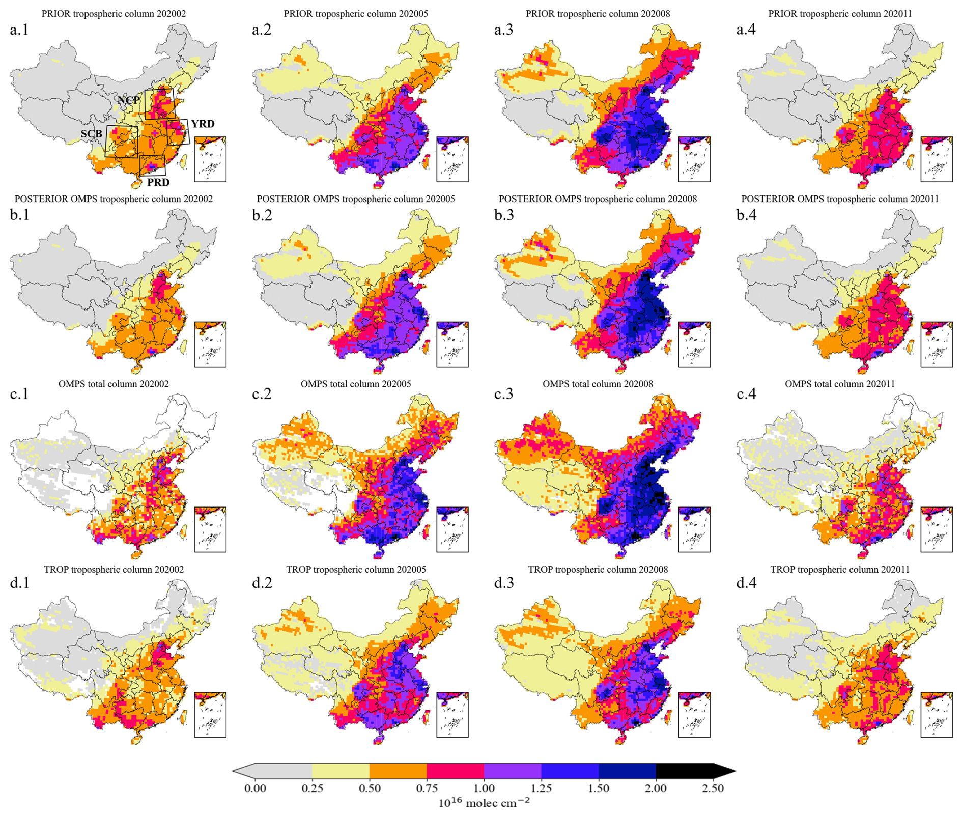
Figure 1 Spatial distributions of formaldehyde columns from GEOS-Chem model-simulated prior tropospheric columns (a) and posterior tropospheric columns constrained by OMPS assimilation (b), satellite observations of OMPS total columns (c), and satellite observations of TROPOMI tropospheric columns (d), both reprocessed to be consistent with the GEOS-Chem shape profile. Panels (a.1)–(d.1), (a.2)–(d.2), (a.3)–(d.3), and (a.4)–(d.4) show February, May, August, and November of 2020, respectively.

2.2 Prior NMVOC emission inventories

The anthropogenic NMVOC emission input into the model mainly comes from the Multi-resolution Emission Inventory for China (MEIC; Zheng et al., 2018). Since the MEIC inventory tailored for the existing chemical species in GEOS-Chem only extends to 2017, the MEIC inventory used in this study is the 2017 emission inventory. This inventory has a spatial resolution of 0.25° latitude × 0.25° longitude and includes industrial, transportation, power generation, and residential emissions. For chemical species used in GEOS-Chem but not included in MEIC and anthropogenic NMVOC emissions outside China, we use the 2019 CEDS global inventory as a supplement. The prior estimates of biogenic NMVOC emissions in this study are obtained from the MEGAN 2.1 model (Guenther et al., 2012). Field straw burning is considered a major seasonal source of NMVOCs in China (Huang et al., 2012; Liu et al., 2015; Stavrakou et al., 2016). In this study, the biomass burning emissions are taken from the GFED version 4 (GFED4) global inventory for 2020 (van der Werf et al., 2017). Before these prior emissions are used to drive GEOS-Chem simulations, the spatial resolution is coarsened to an average value on a 0.5° × 0.625° grid resolution consistent with the model configuration as used in Sect. 2.1.

Figure 2a presents the prior NMVOC emission inventories for 2020, which primarily relies on the anthropogenic emission inventory from MEIC, supplemented by the CEDS inventory for species not included in MEIC. Additionally, biogenic emissions are provided by MEGAN (offline calculation) for the year 2020 with an hourly temporal resolution, directly through the HEMCO emission component of GEOS-Chem; in this study, we did not run the MEGAN model separately. Biomass burning emissions are taken from GFED4. The combination of these three sources is treated as the prior emission inventory used in the following NMVOC emission optimization.

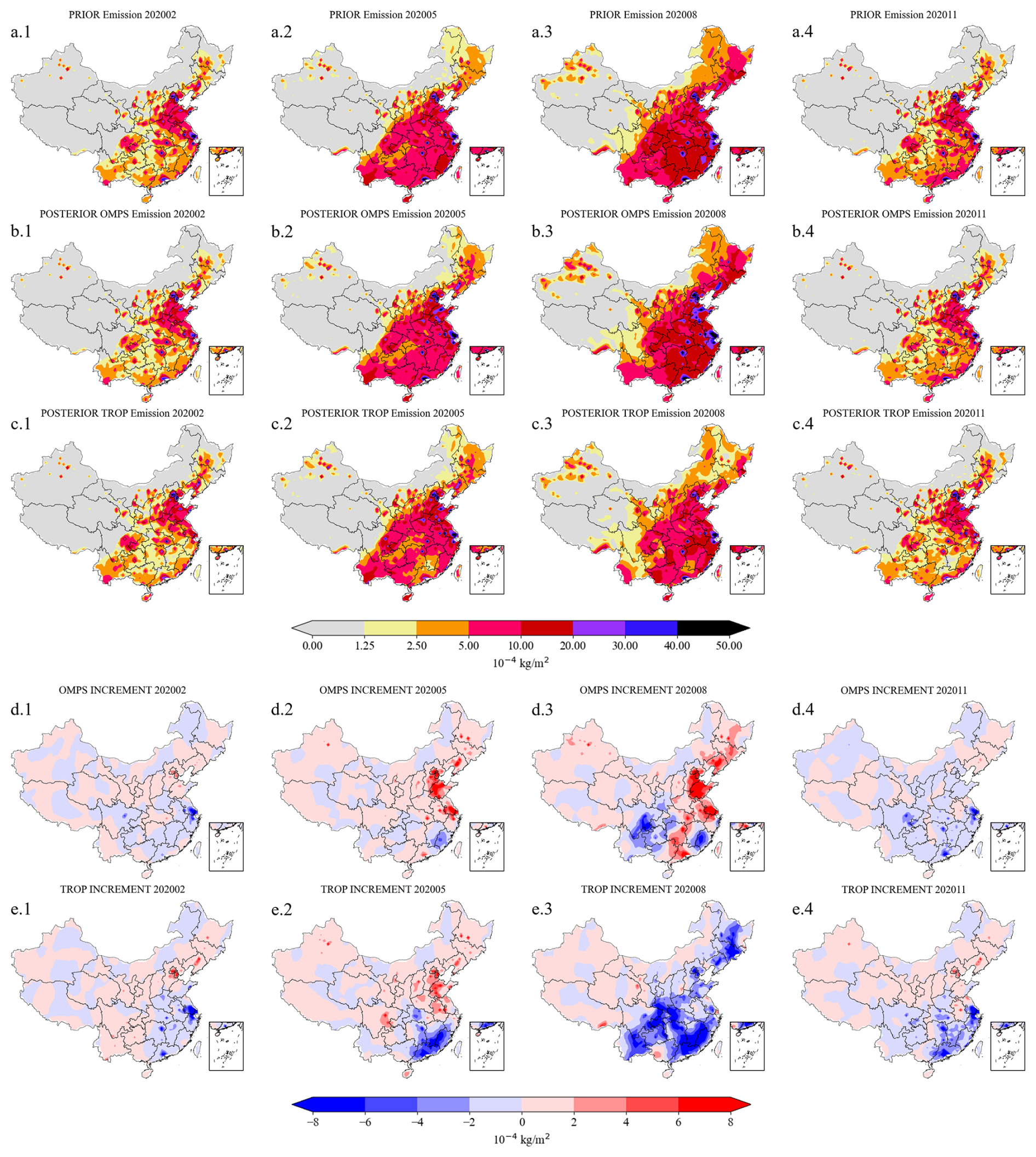
Figure 2 Spatial distributions of the total NMVOC emissions from the prior (a) and posterior (b) results in February (a.1, b.1), May (a.2, b.2), August (a.3, b.3), November (a.4, b.4) 2020. Panels (d.1)–(d.4) and (e.1)–(e.4) show the corresponding emission increments (posterior minus prior) derived from OMPS and TROPOMI assimilation.

2.3 Formaldehyde Satellite measurements

2.3.1 NOAA-20 OMPS

Ozone Mapping and Profiler Suite (OMPS) was launched on Suomi National Polar-orbiting Partnership (SNPP) satellite on 28 October 2011, and on the JPSS-1 satellite (now known as NOAA-20) on 18 November 2017. OMPS/SNPP consists of three instruments: the nadir mapper (OMPS-NM), the profile mapper (OMPS-NP), and the limb profiler (OMPS-LP), while OMPS/NOAA-20 includes only the nadir package (OMPS-NM and OMPS-NP). This study uses OMPS-N20 Level 2 NM formaldehyde Total Column swath orbital Version 1 product (Abad, 2022). OMPS-NM is a hyperspectral nadir viewing spectrometer that measures backscattered light with a spectral resolution of approximately 1 nm. The NOAA-20 spectral measurement range is 300–420 nm. The instrument employs a 2-D CCD array detector in a pushbroom geometry, observing the two-dimensional field below the satellite’s orbit over a swath width of about 2800 km. With 14 or 15 orbits per day, OMPS-NM provides daily global coverage of trace gas columns in the early afternoon local time, with an equatorial crossing time of approximately 13:30. The spatial resolution of OMPS/NOAA-20 was 17 km × 17 km until 13 February 2019, when it was changed to 12 km × 17 km (Flynn et al., 2014; Pan et al., 2017; Seftor et al., 2014).

In this study, the quality control scheme recommended in OMPS product documentation was applied. Data points with formaldehyde column densities exceeding 2×10¹⁷ molec. cm⁻² were excluded to minimize the impact of outliers. After removing outliers, we further excluded data points where the sum of formaldehyde column and twice the observation uncertainty was less than zero. Furthermore, the geometric air mass factors (AMF_G) were defined as follows:

$$\begin{array}{}\text{(1)}& {\mathrm{AMF}}_{\mathrm{G}}=\sec \left(\mathrm{SZA}\right)+\sec \left(\mathrm{VZA}\right)\end{array}$$

Here, SZA represents the solar zenith angle and VZA denotes the viewing zenith angle. Additional data screening was applied by excluding observations with SZA greater than 70°, an air mass factor less than 0.1, a geometric air mass factor greater than 4, a cloud fraction exceeding 0.4, or with positive snow and ice fractions. All screened data were then averaged to a spatial resolution of 0.5° latitude × 0.625° longitude on a monthly basis, consistent with the GEOS-Chem model configuration. To make a fair comparison between the observed and simulation formaldehyde column in the assimilation, we further imposed constraints on the number of observations within each grid cell. Specifically, two filtering schemes were tested, in which grid cells with fewer than 10 or fewer than 50 original observations were excluded. The OMPS formaldehyde columns after applying the threshold of 50 are shown in Fig. 1c, while the results with the threshold of 10 are provided in the Supplement. The differences between the two filtering schemes are minor, particularly across the four study regions considered in this work.

Formaldehyde vertical column densities (VCDs) retrieved from satellite observations are derived using air mass factors (AMF), which strongly depend on the a priori vertical profiles of formaldehyde. Direct comparisons between satellite products and model simulations may be biased if the a priori profiles used in the retrieval differ from the simulated ones. To ensure consistency between the satellite observations and GEOS-Chem simulation, we applied an AMF correction by recalculating the AMF with model-simulated profiles following the method used in Palmer et al. (2001):

$$\begin{array}{}\text{(2)}& \mathrm{AMF}=\underset{p_{\mathrm{s}}}{\overset{\mathrm{0}}{\int }}w\left(p\right)S\left(p\right)\mathrm{d}p\end{array}$$

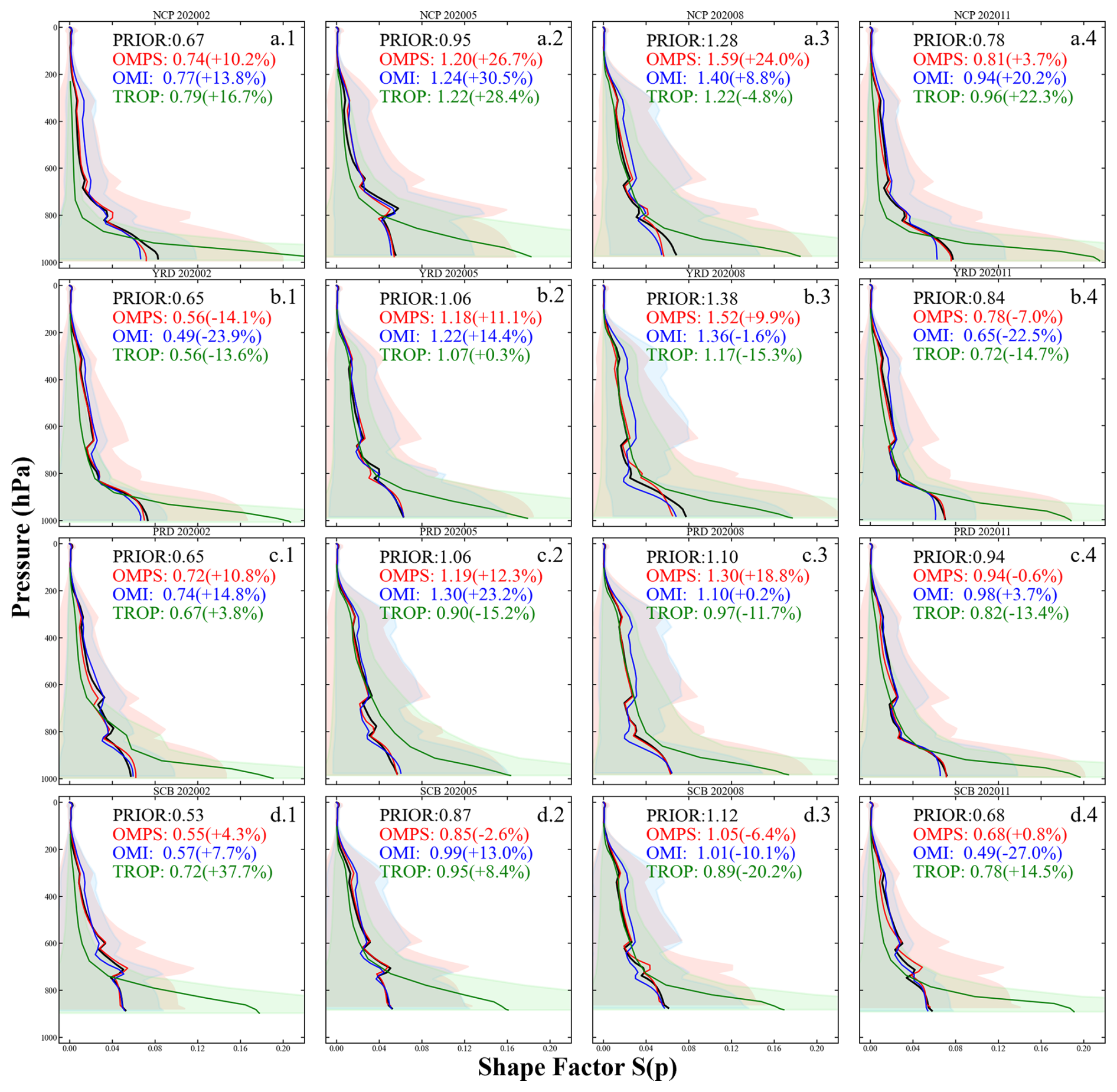
Figure 3 Shape factors of regional-mean formaldehyde columns, as derived from the a priori profiles, followed by normalization, from GEOS-Chem model-simulated prior (black) and satellite observations by OMPS (blue), TROPOMI (red), and OMI (green). Panels (a)–(d) correspond to the North China Plain, Yangtze River Delta, Pearl River Delta, and Northeast China, respectively. Sub-panels (a.1)–(d.1), (a.2)–(d.2), (a.3)–(d.3), and (a.4)–(d.4) represent February, May, August, and November 2020, respectively. Values in parentheses indicate the biases of satellite observations relative to the prior simulation. Shaded areas denote the observational uncertainties.

The right-hand side of the equation represents the vertically integrated product of the scattering weight w(p) and the shape factor S(p) as a function of pressure p, where w(p) characterizes the sensitivity of the satellite measurement to a given atmospheric layer and S(p) describes the normalized vertical profiles of the a priori profiles. The scattering weights w(p) are primarily determined by satellite observational geometry (e.g., solar and viewing zenith angles), surface albedo, and cloud fraction, while the shape factor S(p) depends on the vertical profiles of formaldehyde. The integration is performed over the pressure coordinate from the surface (p_s) to the top of the atmosphere. Figure 3 illustrates the vertical distribution of the shape profile, highlighting the relative contributions of different layers. The vertical column density (VCD) is obtained from the ratio of the slant column density (SCD) to the AMF:

$$\begin{array}{}\text{(3)}& \mathrm{VCD}={\displaystyle \frac{\mathrm{SCD}}{\mathrm{AMF}}}\end{array}$$

In the OMPS formaldehyde product, the SCD is derived as the sum of three components: the fitted differential slant column amount (ΔSCD), the reference sector correction (SCD_Ref), and the bias correction (SCD_B):

$$\begin{array}{}\text{(4)}& \mathrm{SCD}=\mathrm{\Delta }\mathrm{SCD}+{\mathrm{SCD}}_{\mathrm{Ref}}+{\mathrm{SCD}}_{\mathrm{B}}\end{array}$$

Here, ΔSCD represents the differential slant column amount retrieved from the DOAS spectral fitting, SCD_Ref is the reference sector correction that accounts for background contributions and instrumental offsets by using clean reference regions, and SCD_B denotes an additional bias correction to mitigate systematic errors.

The OMPS observations were assimilated as total columns after re-calculation of the air mass factor using GEOS-Chem shape profiles for consistency with the model vertical profile. These reprocessed total columns are shown in Fig. 1c.1–c.4. The original a priori shape factors used in the official satellite products (before reprocessing) are displayed as red lines in Fig. 3.

2.3.2 Sentinel-5P TROPOMI

Sentinel-5 Precursor (Sentinel-5P) is a member of the European Space Agency's (ESA) Sentinel satellite series. It is in a low-Earth afternoon polar orbit with a swath of 2600 km, allowing for daily global coverage (Veefkind et al., 2012). Its sole payload is Tropospheric Monitoring Instrument (TROPOMI), a nadir-viewing, 108° field-of-view push-broom grating hyperspectral spectrometer. TROPOMI covers the ultraviolet-visible (UV-VIS, 270 to 495 nm), near-infrared (NIR, 675 to 775 nm), and shortwave infrared (SWIR, 2305 to 2385 nm) spectral ranges. Its Level 2 products include vertical columns of ozone, sulfur dioxide, nitrogen dioxide, formaldehyde, carbon monoxide, and methane, as well as ozone profiles, aerosol layer height, cloud information, and aerosol index. The initial spatial resolution was 3.5 km × 7 km, which was improved to 3.5 km × 5.5 km on 6 August 2019.

The retrieval algorithm for TROPOMI formaldehyde is based on the DOAS method and is directly inherited from the OMI QA4ECV product retrieval algorithm (De Smedt et al., 2017). This study uses the Sentinel-5P TROPOMI Level 2 Tropospheric formaldehyde Version 2 product (Copernicus Sentinel data processed by ESA and DLR, 2020). Vigouroux et al. (2020) evaluated this TROPOMI formaldehyde product using ground-based solar-absorption FTIR (Fourier-transform infrared) measurements, demonstrating its good quality. De Smedt et al. (2021) further assessed TROPOMI formaldehyde using OMI observations and MAX-DOAS network column measurements, also showing favorable results. When using Level 2 TROPOMI formaldehyde data for the validation in this study, we applied the recommended quality assurance filtering by retaining only pixels with a qa value greater than 0.5. This criterion ensures the exclusion of error flags and requires that the cloud radiance fraction at 340 nm is below 0.5, the solar zenith angle (SZA) does not exceed 70°, the surface albedo is below 0.2, no snow or ice warning is present, and the air mass factor (AMF) is larger than 0.1. The operational TROPOMI HCHO Level-2 product provides tropospheric vertical columns together with averaging kernels and a priori profiles defined on 34 vertical layers (from the surface to ∼ 0.1 hPa). Because stratospheric formaldehyde is negligible (De Smedt et al., 2018, 2021), we directly use the reported tropospheric columns in this study without reconstructing total columns. After filtering, the TROPOMI observations were aggregated to monthly means on a 0.5° × 0.625° grid, ensuring consistency with the resolution used in the GEOS-Chem simulations. In addition, we further constrained the number of observations per grid cell: Fig. 1d shows the results after excluding grid cells with fewer than 50 observations, while the results with a threshold of 10 are also provided in the Supplement. The differences between the two filtering schemes are minor, particularly over the study regions.

Beyond the recommended quality filtering, a critical consideration when comparing TROPOMI formaldehyde retrievals with model simulations is the sensitivity of the retrieved columns to the a priori vertical profile assumed in the retrieval algorithm. In this study, OMPS and OMI formaldehyde products are harmonized with the model by recalculating the AMF using GEOS-Chem shape factors, following the conventional approach. For TROPOMI, the officially provided averaging kernels (AVK) are applied instead. Importantly, these two correction strategies are mathematically equivalent. The averaging kernel represents the ratio of the altitude-resolved sensitivity to the total AMF used in the operational retrieval. Consequently, convolving the model profile with the AVK and adding the same background column yields identical results to recalculating the total AMF with the model profile and applying it to the slant column, provided that the background correction and a priori profile replacement are handled consistently (Palmer et al., 2001; Eskes and Boersma, 2003; Boersma et al., 2004; De Smedt et al., 2021). Both approaches achieve the same objective: removing the influence of the satellite’s a priori profile and replacing it with the GEOS-Chem profile, thereby ensuring observational–model consistency prior to assimilation. The AVK application for TROPOMI employed here follows the methodology established for the IASI NH₃ version 4 product (Clarisse et al., 2023; Xia et al., 2025). The corrected column is calculated as:

$$\begin{array}{}\text{(5)}& {\widehat{X}}^{\mathrm{m}}={\displaystyle \frac{{\widehat{X}}^{\mathrm{a}}-B}{{\sum }_p{A}_p^{\mathrm{a}}{m}_p}}+B\end{array}$$

where ${\widehat{X}}^{\mathrm{m}}$ denotes the formaldehyde column adjusted with the model profile, ${\widehat{X}}^{\mathrm{a}}$ is the retrieved column based on the a priori profile, and B is the background concentration. The term $A_p^{\mathrm{a}}$ represents the AVK at pressure level p, and m_p is the normalized model shape factor at the same level, defined as:

$$\begin{array}{}\text{(6)}& m_p={\displaystyle \frac{M_p^{\mathrm{m}}-B_p}{M^{\mathrm{m}}-B}}\end{array}$$

The TROPOMI tropospheric columns were assimilated after application of GEOS-Chem shape profiles. These reprocessed tropospheric columns are shown in Fig. 1d.1–d.4, with their vertical shape factors shown in Fig. 3 (green line) to illustrate the normalized contribution of each pressure layer to the tropospheric columns. We adopted tropospheric rather than total columns because the retrieval product itself provides tropospheric columns.

2.3.3 Aura OMI

The Ozone Monitoring Instrument (OMI) is an important satellite instrument onboard the Aura satellite, launched on 15 July 2004, with the objective of monitoring atmospheric gases, aerosols, and clouds to improve our understanding of atmospheric chemistry and climate change. OMI provides daily global coverage with a wide swath of 2600 km and a spatial resolution of approximately 13 × 24 km at nadir, with an equator crossing time of about 13:45 LT. The sensor contains three spectral channels (UV-1, UV-2, and VIS), covering the wavelength ranges of 264–311, 307-383, and 349-504 nm, respectively, which enable the retrieval of key trace gases including O₃, NO₂, SO₂, and formaldehyde (Levelt et al., 2006, 2018).

In this study, we use the OMI/Aura formaldehyde Total Column Daily L2 Global Version 3 product (Chance, 2014). In order to minimize the influence of poor-quality data, we applied strict quality filtering. Only pixels with cloud fraction ⩽ 0.3, solar zenith angle ⩽ 70°, and a main data quality flag = 0 were retained. To avoid poor-quality measurements at large pixel sizes, the five marginal pixels on each side of the swath were discarded, and only pixels within rows 6–55 were used (Zhu et al., 2017; Xue et al., 2020). Because OMI has experienced a row anomaly since 2007, pixels with Xtrack quality flags = 0 were further selected to eliminate its impact. Additionally, given the large uncertainties in formaldehyde retrievals, pixels with a fitting root mean square (RMS) ⩽ 0.003 were retained to remove most outliers (Souri et al., 2017).

The OMI observations are then aggregated to monthly means on a 0.5° × 0.625° grid, consistent with the GEOS-Chem model resolution. To ensure sufficient sampling per grid cell, we also applied two filtering schemes based on the number of observations, excluding grid cells with fewer than 10 or fewer than 50 valid pixels. Unlike OMPS and TROPOMI, however, OMI shows a strong reduction in data coverage under these constraints, and the product becomes sparse after applying the threshold of 50 observations. This indicates that OMI suffers from insufficient sampling density in China for high-resolution assimilation. The vertical profile correction of OMI formaldehyde was conducted using the same approach as applied to OMPS, by recalculating AMF with model-simulated vertical profiles. The resulting OMI columns after profile correction and the two data-volume filters are shown in Fig. S3.

2.4 Ozone ground station observation

This study aims to constrain the NMVOC emissions in China by assimilating multiple formaldehyde satellite products. As aforementioned, formaldehyde is an important precursor to ozone, the optimization of the NMVOC emission inventories and concentrations are supposed to improve the ozone simulation simultaneously. To evaluate the magnitude and quality of this impact, the ground level ozone concentrations from the National Urban Air Quality Real-time Publishing Platform of the China National Environmental Monitoring Center (CNEMC, last access: 15 May 2024) are used in the validation. The ozone measurements utilized in this study are from 1602 sites across China. The MDA8 values of surface ozone observations are calculated based on the hourly data before they are compared against the model simulation. Results of the comparison will be described in Sect. 3.4.

2.5 Assimilation algorithm

This study employs the four-dimensional ensemble variational (4DEnVar) methodology to optimize NMVOC emissions with satellite formaldehyde observations. The goal of the assimilation is to find the most likely estimate of the state vector, which is the monthly NMVOC emission inventories f over the entire model domain. Note that f represents the vector of total NMVOC emissions, rather than separately gridded anthropogenic, biogenic, or biomass burning VOC emissions. To optimize emissions from these three sectors, additional observations or a well-defined spatial correlation structure are required, which are not available in this study. The prior estimate f_b is from the inventories described in Sect. 2.2, and the formaldehyde observations y are described in Sect. 2.3. Mathematically, assimilation is performed via minimizing the cost function J as follows:

$$\begin{array}{}\text{(7)}& \begin{array}{rl}\mathcal{J}\left(\mathit{f}\right)& ={\displaystyle \frac{\mathrm{1}}{\mathrm{2}}}(\mathit{f}-{\mathit{f}}_{\mathrm{b}}{)}^T{\mathbf{B}}^{-\mathrm{1}}(\mathit{f}-{\mathit{f}}_{\mathrm{b}})\\ & +{\displaystyle \frac{\mathrm{1}}{\mathrm{2}}}{\left\{\mathit{y}-\mathcal{H}\mathcal{M}\left(\mathit{f}\right)\right\}}^T{{\mathbf{O}}^{-}}^{\mathrm{1}}\left\{\mathit{y}-\mathcal{H}\mathcal{M}\left(\mathit{f}\right)\right\}\end{array}\end{array}$$

The cost function 𝒥 is the sum of two parts: background and observation penal term. The background term quantifies the difference between the optimal f and the prior emission inventories f_b, while the observation term calculates the difference between the simulation driven by f and the satellite observations y. In addition to the f_b that represents the prior NMVOC emission vector calculated from the anthropogenic, biogenic, and biomass burning sources as been illustrated in Sect. 2.2. The uncertainty in the NMVOCs simulation is assumed to be attributed to errors in the emission inventories, and can be compensated using a spatially varying tuning factor α:

$$\begin{array}{}\text{(8)}& f\left(i\right)=f_{\mathrm{b}}\left(i\right)\cdot \mathit{\alpha }\left(i\right)\end{array}$$

in here f_b(i) denotes the NMVOC emission rate in the given grid cell i. The α values are defined to be random variables with a mean of 1.0, a minimum of 0.1 and a standard deviation of 0.4, corresponding to a uniform 120 % uncertainty applied to the total NMVOC emissions rather than sector-specific settings as adopted in previous studies (Choi et al., 2022; Jung et al., 2022; Souri et al., 2020). The rationale for this choice is provided in the Supplement. This empirical value was found to provide sufficient spaces for resolving the observation-minus-simulation errors. A background covariance B_α is formulated as a product of the constant standard deviation and a spatial correlation matrix C:

$$\begin{array}{}\text{(9)}& {\mathbf{B}}_{\mathit{\alpha }}\left(i,j\right)={\mathit{\sigma }}_{\mathit{\alpha }}\cdot \mathbf{C}\left(i,j\right)\end{array}$$

where C(i,j) represents a distance-based spatial correlation between two αs in the grid cell i and j, and is defined as:

$$\begin{array}{}\text{(10)}& \mathbf{C}\left(i,j\right)=e^{-(d_{i,j}/l{)}^{\mathrm{2}}/\mathrm{2}}\end{array}$$

where d_i,j represents the distance between two grid cells i and j. l here denotes the correlation length scale which controls the spatially variability freedom of the αs. A small value of l indicates that the tuning factors αs are less spatially correlated, thereby enabling emission optimization at a finer spatial scale. However, this also necessitates a larger number of ensemble runs to adequately represent the model realization from emission to simulation. An empirical parameter l=300 km which is used in Jin et al. (2023) to nudge the ammonia emission that has a rapid spatially variability is also taken in this study. With the covariance matrix B_α, the NMVOC emission background covariance B is obtained via a Schur Product:

$$\begin{array}{}\text{(11)}& \mathbf{B}={\mathbf{B}}_{\mathit{\alpha }}\circ \mathbf{C}\end{array}$$

In the observation term, y is the observation vector, representing satellite observations, ℳ is the GEOS-Chem model driven by emissions f, ℋ is the observation operator that transfers the three-dimensional concentration into the observational space, and O is the observation covariance matrix. In this study, the assimilated observations include the OMPS total columns and TROPOMI tropospheric columns. A distinct observation operator ℋ is configured to enable a fair comparison of the observation-minus-simulation mismatch. The satellite formaldehyde observations are assumed to be independent, therefore O is a diagonal matrix. The diagonal value here is calculated as:

$$\begin{array}{}\text{(12)}& {\mathit{\sigma }}_{\text{total}}=\sqrt{{\mathit{\sigma }}_{\text{instrument}}^{\mathrm{2}}+{\mathit{\sigma }}_{\text{represent}}^{\mathrm{2}}}\end{array}$$

In Eq. (12), σ_total is defined as the total uncertainty, which is the square root of the sum of the squares of the instrument uncertainty σ_instrument from the formaldehyde observations and the representative uncertainty σ_represent introduced when processing the data into monthly averages. The representative uncertainty σ_represent is represented by the standard deviation of the data. The spatial distribution of the total uncertainty is provided in Fig. S2 in the Supplement.

The assimilation methodology used in this paper is the four-dimensional ensemble variational (4DEnVar). Different from the classic 4DVar that requires adjoint in the cost function minimization, 4DEnVar emulates the GEOS-Chem formaldehyde simulating model using an ensemble-based linear approximation and hence is adjoint-free. The method is first proposed by Liu et al. (2008) and successfully implemented in our recent dust aerosol (Jin et al., 2021) and ammonia emission inversion (Jin et al., 2023; Xia et al., 2025). The detailed procedures for minimizing the cost function Eq. (7) are illustrated in section “Minimization of the Cost Function in 4DEnVar” in the Supplement.

3 Results and discussion

This section first presents the three satellite observations evaluation in terms of the vertical profile structure, qualified-data volume and monthly mean biases. Independent assimilations are then performed by either assimilating the OMPS or assimilating the TROPOMI retrievals independently. Posterior of the NMVOC emission, formaldehyde column results and the impact on ozone simulation are discussed. A consistency analysis is introduced to assess the reliability of the two posterior emission.

3.1 Satellite data evaluation

Figure 3 shows the vertical profiles of formaldehyde shape factors used to compute the reported satellite vertical columns before any model-based profile correction is applied. Both the OMI and OMPS retrievals use GEOS-Chem model outputs as their a priori profiles (González Abad et al., 2015, 2016; Nowlan et al., 2023). Consequently, their shape factors are highly similar. formaldehyde shape factors generally decrease with altitude but exhibit characteristic peaks and troughs: a minimum at 750–850 hPa, a first peak ∼ 30 hPa above it, a second prominent peak at 600–700 hPa, and a third peak near 350 hPa that is strongest in April and August and weaker in January and November. Above 350 hPa, shape factor decay toward zero. These features agree well with previously reported formaldehyde profile shapes over China (Zhu et al., 2016, 2020). Overall, the OMPS profile most closely matches GEOS-Chem, whereas OMI shows slight peak shifts or spurious upper-level enhancements in some regions, particularly during May and August.

In contrast, the operational TROPOMI retrieval uses the a priori profiles from the TM5-MP model (De Smedt et al., 2018, 2021), which places substantially more mass near the surface. This results in a markedly different vertical structure: an approximately logarithmic monotonic decrease with altitude, with only minor perturbations over SCB (∼ 300 hPa) and PRD (∼ 800 hPa) and very high near-surface shape factor. These differences in a priori profile shape are the primary reason why profile correction is essential for meaningful satellite–model comparisons (Eskes and Boersma, 2003).

Additionally, Fig. 3 clearly shows that stratospheric formaldehyde ($>\sim$ 200 hPa) can be largely neglected in both the GEOS-Chem simulation and the OMPS and TROPOMI retrievals (González Abad et al., 2015; De Smedt et al., 2018). Because the stratospheric contribution is negligible and no explicit stratospheric correction is applied in either retrieval, we hereafter use the term ”formaldehyde column” without distinguishing between total and tropospheric columns in subsequent discussion.

Uncertainty is a key component in the assimilation process and serves as a crucial indicator of satellite data quality. Fig. 3 illustrates the vertical distribution of retrieval uncertainties. In the mid- to upper troposphere (200–600 hPa), OMPS and OMI show comparable levels of uncertainty. However, below 600 hPa, OMPS uncertainties become substantially larger, likely due to cloud contamination and retrieval algorithm approximations (González Abad et al., 2016; Nowlan et al., 2023). As shown in Supplement Fig. S2, the overall uncertainty of OMPS is significantly higher than that of the other two satellite datasets. At first glance, OMI data may appear superior, but this advantage largely results from strict filtering, which excludes a substantial fraction of problematic data. As illustrated in Supplement Fig. S3a, b, applying a threshold of 50 observations per grid cell drastically reduces spatial coverage, rendering OMI unsuitable for national-scale assimilation. Previous studies that assimilated OMI over China have typically interpolated the data to coarser resolutions to ensure applicability (Cao et al., 2018; Miyazaki et al., 2020). Therefore, only OMPS and TROPOMI formaldehyde columns are assimilated in this study, while OMI is excluded for our high-resolution emission inversion due to the poor data coverage.

Figure 3 also presents satellite retrieval deviations from the prior model estimates. When all three satellite datasets exhibit the same sign of deviation (positive or negative) relative to the model, they are considered consistent. Such consistency is observed, for example, in February, May, and November over NCP and in February over PRD and SCB, where all three datasets show positive deviations; and in February and November over YRD and in August over SCB, where all show negative deviations. These cases indicate stronger reliability. In other situations, when OMPS and TROPOMI exhibit the same bias direction, they are also considered consistent, as in November over PRD and SCB. Overall, 10 out of 16 cases (62.5 %) exhibit consistency, with higher coherence primarily occurring in the cold season and during spring and autumn months over NCP and SCB. Subsequent analyses will explicitly consider this consistency to enhance the robustness of the conclusions.

3.2 NMVOC emissions

The spatial characteristics of the NMVOC emissions in 2020 are clearly shown in Fig. 2 which presents the spatial distribution of four monthly average emissions from the prior simulation (a.1–a.4) and the posterior estimates constrained by OMPS (b.1–b.4) and TROPOMI (c.1–c.4) formaldehyde observations. Significant emission increments relative to the prior estimates are mainly concentrated in eastern and southern China. In most regions, the posterior results constrained by OMPS (d.1–d.4) and TROPOMI (e.1-e.4) exhibit broadly consistent adjustment patterns. However, notable differences between the two posterior estimates can still be observed, particularly over eastern China in August and southern China in May. The results reveal pronounced seasonal variability and regional heterogeneity in emission intensity, with the NCP, YRD, PRD, and SCB identified as major emission hotspots throughout the year.

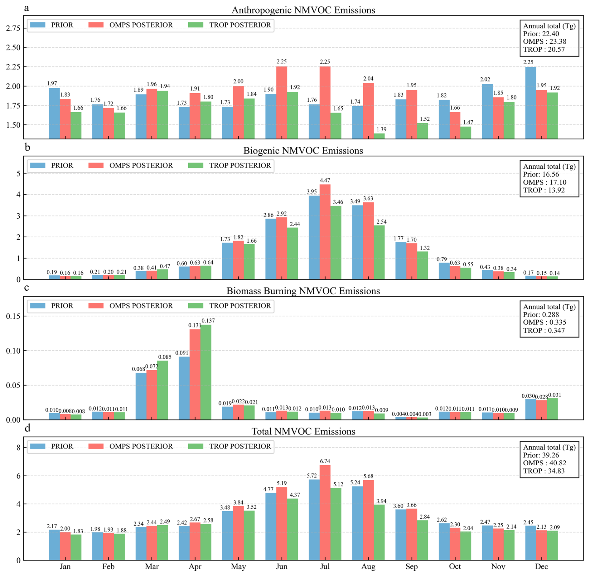
Figure 4 Monthly NMVOC emissions in 2020 from the prior simulation (blue) and the posterior simulations constrained by assimilating OMPS (red) and TROPOMI (green) formaldehyde observations. Panels show anthropogenic emissions (a), biogenic emissions (b), biomass burning emissions (c), and total emissions (d). The annual totals for each category are indicated in the legends.

Although the major high-emission regions can be clearly identified, the complexity of emission source types and the wide range of emission magnitudes render the maps visually dense, making it difficult to directly interpret regional characteristics and seasonal changes. Therefore, subsequent analyses are focused on these four representative regions to enable a more detailed investigation. Figure 4 further displays the monthly and annual totals of NMVOC emissions across China in 2020. In general, the two posterior estimates exhibit good agreement for most months. Specifically, both show consistent decreases during January, February, and October to December, while simultaneous increases are observed from March to May. But notable discrepancies are observed during the June–September period, which account for approximately 83 % of the total annual difference between the two posterior datasets – with July and August alone contributing around 56 %. This leads to different estimates of annual emissions: the annual total constrained by OMPS assimilation is estimated at 40.82 Tg, while that constrained by TROPOMI is 34.83 Tg, both differing from the prior estimate of 39.26 Tg. To more accurately assess the regional emission responses under different observational constraints, the consistent and inconsistent months are discussed separately in the following sections.

In months with high consistency, January–February, during the transition from winter to spring, both assimilation results show a reduction in emissions, with anthropogenic emissions exhibiting a particularly significant decline. This may be because the emission inventory includes winter heating emissions, while the actual heating demand has been reduced due to global warming, resulting in an overestimation (Lu et al., 2025; Xu et al., 2025). In spring, March-May, emissions gradually increase, likely driven by enhanced biogenic emissions due to rising temperatures and vigorous vegetation growth (Guenther et al., 1995; Monson et al., 2012). After November, as the season shifts from autumn to winter, emissions decline again, with notable fluctuations in biogenic emissions in October, though anthropogenic emissions remain the primary contributor to the overall trend. In the inconsistent months (June–September, corresponding to summer and autumn), discrepancies arise between OMPS and TROPOMI results. These differences may arise from variations in emission characterization during summer, marked by strong convection, high humidity, and elevated cloud and aerosol content, which differentially impact the retrieval of optical depth and columns by OMPS and TROPOMI.

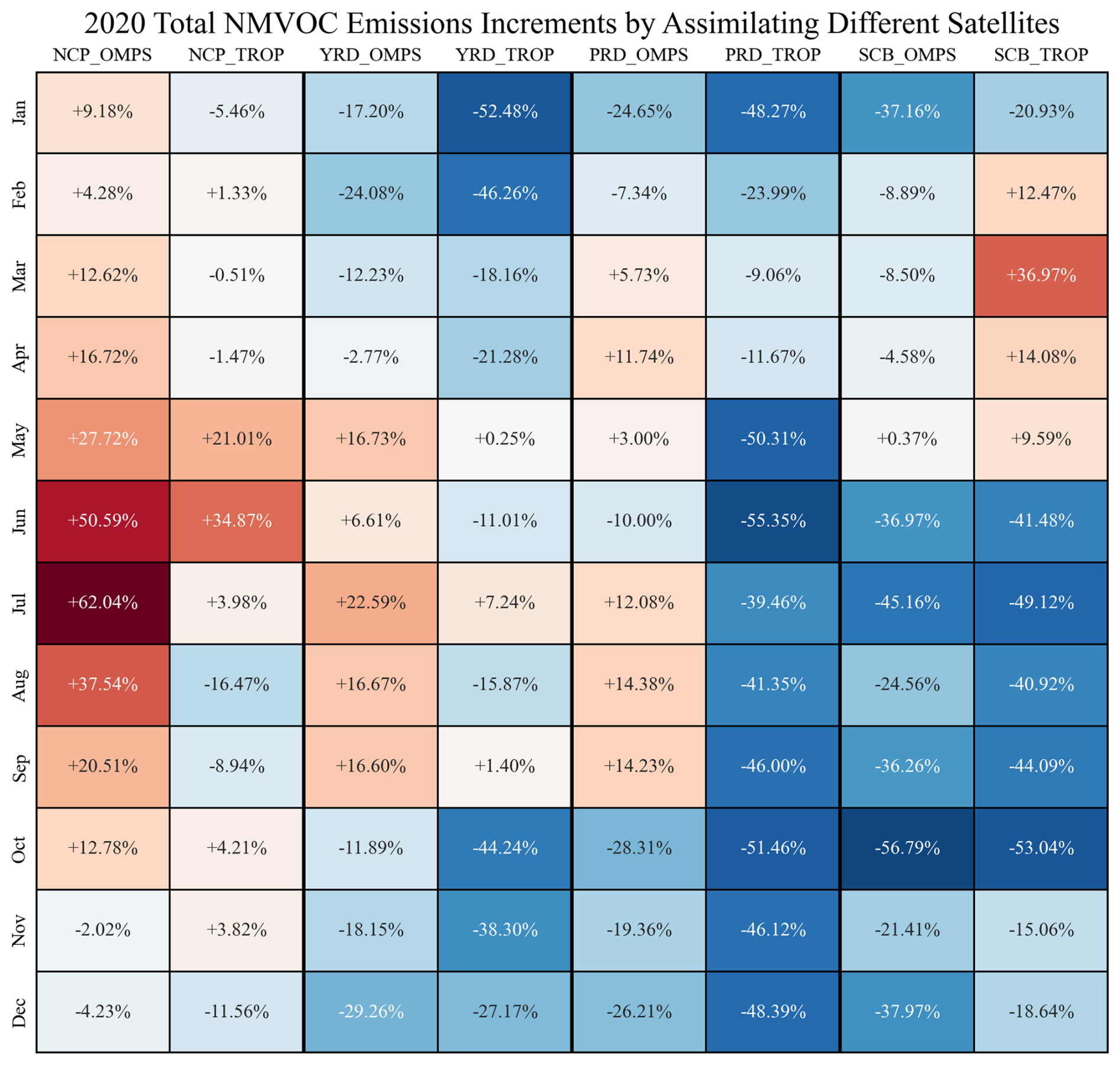
Figure 5 Monthly increments in total NMVOC emissions between the posterior and prior simulations derived from the assimilation of OMPS and TROPOMI formaldehyde observations over four key regions of China: the North China Plain, Yangtze River Delta, Pearl River Delta, and Sichuan Basin in 2020. Positive values indicate an increase in posterior emissions relative to the prior, while negative values indicate a decrease.

A clear regional divergence in NMVOC emission increments after assimilation is revealed in Fig. 5, with further analysis highlighting the sources of these discrepancies. In the NCP, OMPS assimilation results for July indicate a significant emission increase of 62.04 %, while TROPOMI shows a smaller increase. In August and September, the two datasets exhibit opposing trends. In contrast, increment differences are relatively minor in March–April, with OMPS assimilation results showing an increase of approximately 14 %, while TROPOMI remains largely unchanged. During January–February and November-December, both datasets display minimal changes. Overall, the prior inventory for the NCP appears underestimated in May–June. In the YRD, except for May and July, other months (e.g., June, August, and September) show opposing trends. In the PRD, nearly all months from March to September are classified as inconsistent. However, both regions demonstrate consistent emission reductions during the cold season, suggesting an overestimation in the a priori emission inventory for winter. In the SCB, negative emission increments during the warm season are particularly pronounced, generally exceeding 20 %, with reductions in June–July surpassing 35 %. During the cold season (January and October–December), both datasets show consistent declines with comparable values. Months with lower consistency are primarily concentrated in February-May, indicating a likely overestimation in the a priori emission inventory for this region.

In 2020, anthropogenic emissions in China were influenced by the COVID-19 pandemic, leading to observable changes. To better evaluate the general applicability of the proposed method, it is also necessary to conduct a comparative analysis for the pre-pandemic year of 2019. Fig. S5 in the Supplement presents the total NMVOC emission increments for the four major regions in 2019, based on data assimilation of OMPS and TROPOMI observations. In the NCP region, strong consistency is again observed in June, with posterior emissions increasing by 57.71 % and 30.09 % from OMPS and TROPOMI assimilation, respectively, further confirming the underestimation of prior emissions in this period. In the YRD, February, October, and November are identified as consistent months, aligning with the consistent periods in 2020, suggesting a likely overestimation in the prior inventory during these months. In the PRD region, consistency is found in January, February, June, July, November, and December, while in the SCB region, it occurs in January and from April to December. These consistent months largely overlap with those in 2020, though some differences are evident. For example, June and July emerge as new consistent months in PRD, while October and November remain consistent but exhibit notably smaller emission decreases compared to 2020. In SCB, April and May appear as additional consistent months, while the remaining consistent periods continue to exhibit decreases in emissions. Notably, from June to November, the two posterior datasets show an average decrease of 42.26 % compared to the prior emissions, indicating a high probability of overestimation in the prior inventory for this region during that period.

3.3 Formaldehyde columns evaluation

The spatial distributions of formaldehyde columns in February, May, August, and November 2020 are shown in Fig. 1. Panels (a.1)–(a.4) display the prior simulations of formaldehyde columns, (b.1)–(b.4) present the posterior simulations of formaldehyde columns assimilated by OMPS, (c.1)–(c.4) show the OMPS satellite observations of formaldehyde columns, and (d.1)–(d.4) illustrate the TROPOMI satellite observations of formaldehyde columns. In addition, the prior and posterior simulations of formaldehyde columns for 2020 are also provided in the Supplement Fig. S7. Regarding the spatial patterns, high formaldehyde columns in February are concentrated in the NCP, YRD, and PRD regions, with the posterior results showing an expanded high-value area in the NCP but a reduced coverage in the YRD. In May, overall formaldehyde columns increase nationwide, with particularly pronounced growth in the NCP and PRD. In August, formaldehyde columns increase in the NCP, YRD, and PRD, while they decrease in the SCB. In November, the changes are modest, but all four regions exhibit reduced formaldehyde columns.

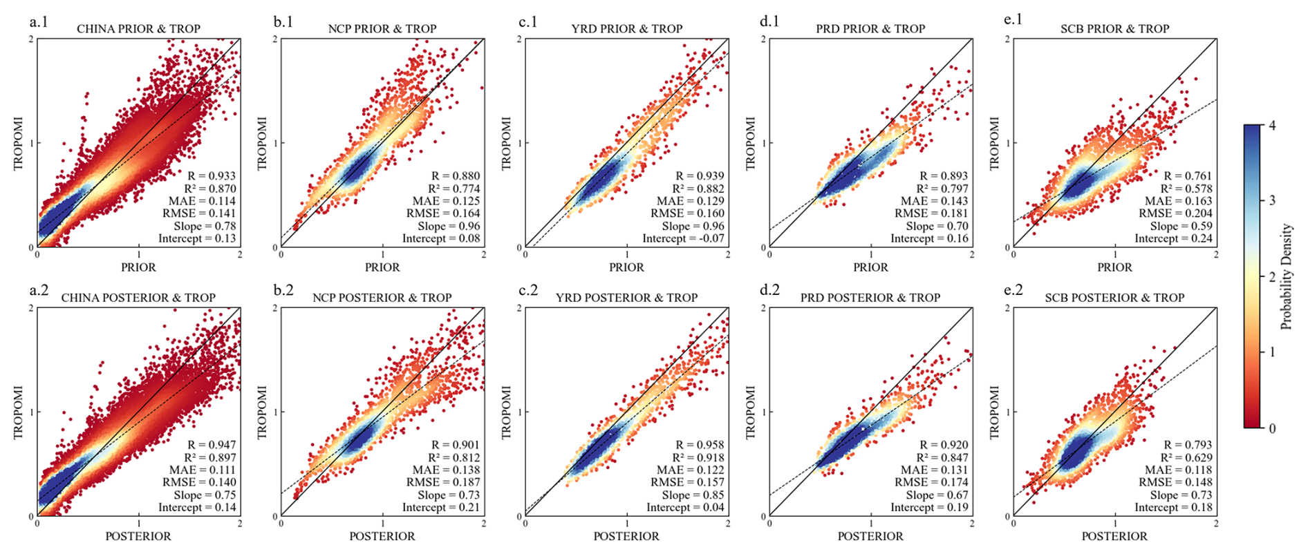
Figure 6 Scatter density plots comparing GEOS-Chem simulated formaldehyde columns with TROPOMI observations in 2020. Panels (a.1)–(e.1) show comparisons between prior simulations and TROPOMI, while panels (a.2)–(e.2) show comparisons between posterior simulations constrained by assimilating OMPS observations and TROPOMI. The regions considered are China (a), the North China Plain (b), the Yangtze River Delta (c), the Pearl River Delta (d), and the Sichuan Basin (e). The probability density of the data points is indicated by the color scale. The correlation coefficient (R), coefficient of determination (R²), mean absolute error (MAE), root mean square error (RMSE), regression slope, and intercept are reported in each panel.

The prior and OMPS-driven posterior simulations of formaldehyde columns were compared with the TROPOMI formaldehyde columns to evaluate the changes in formaldehyde. Scatter plots together with statistical metrics (R², R, MAE, and RMSE) for the whole country and four subregions in 2020 are presented in Fig. 6. The prior simulation already shows reasonably good performance (a.1)–(e.1), with most points distributed close to the 1:1 line and exhibiting strong correlations with observations. Nevertheless, further improvements are still possible. After assimilating OMPS data, the posterior results compared with TROPOMI show higher R² values across all regions, indicating strengthened correlations. For China and NCP, the improvements are comparable, with R² increasing by about 0.027 (from 0.870 to 0.897 for China, and from 0.774 to 0.812 for NCP). In the YRD, the improvement is more pronounced, with R² rising from 0.882 to 0.918, and the scatter around the regression line substantially reduced, with many outliers corrected. The most significant improvements occur in PRD and SCB, where R² increases by approximately 0.05. In these regions, the overestimations present in the prior simulations are effectively mitigated, particularly for high-value cases. In terms of RMSE and MAE, decreases are observed in all regions except NCP. A comparison between Figures (b.1) and (b.2) indicates improvements in the low- and mid-value ranges, whereas substantial overestimations appear in the high-value range. This issue is likely related to the instrumental errors of OMPS observations, as discussed in Sects. 2.3.1 and 3.2, which introduce considerable uncertainties.

Figure 7 Monthly mean formaldehyde columns in 2020 from the prior simulation (gray), posterior simulations constrained by assimilating OMPS (black dashed) and TROPOMI (black dotted) observations, and satellite observations from OMPS (blue) and TROPOMI (green). Panels show results over China (a), the North China Plain (b), the Yangtze River Delta (c), the Pearl River Delta (d), and the Sichuan Basin (e).

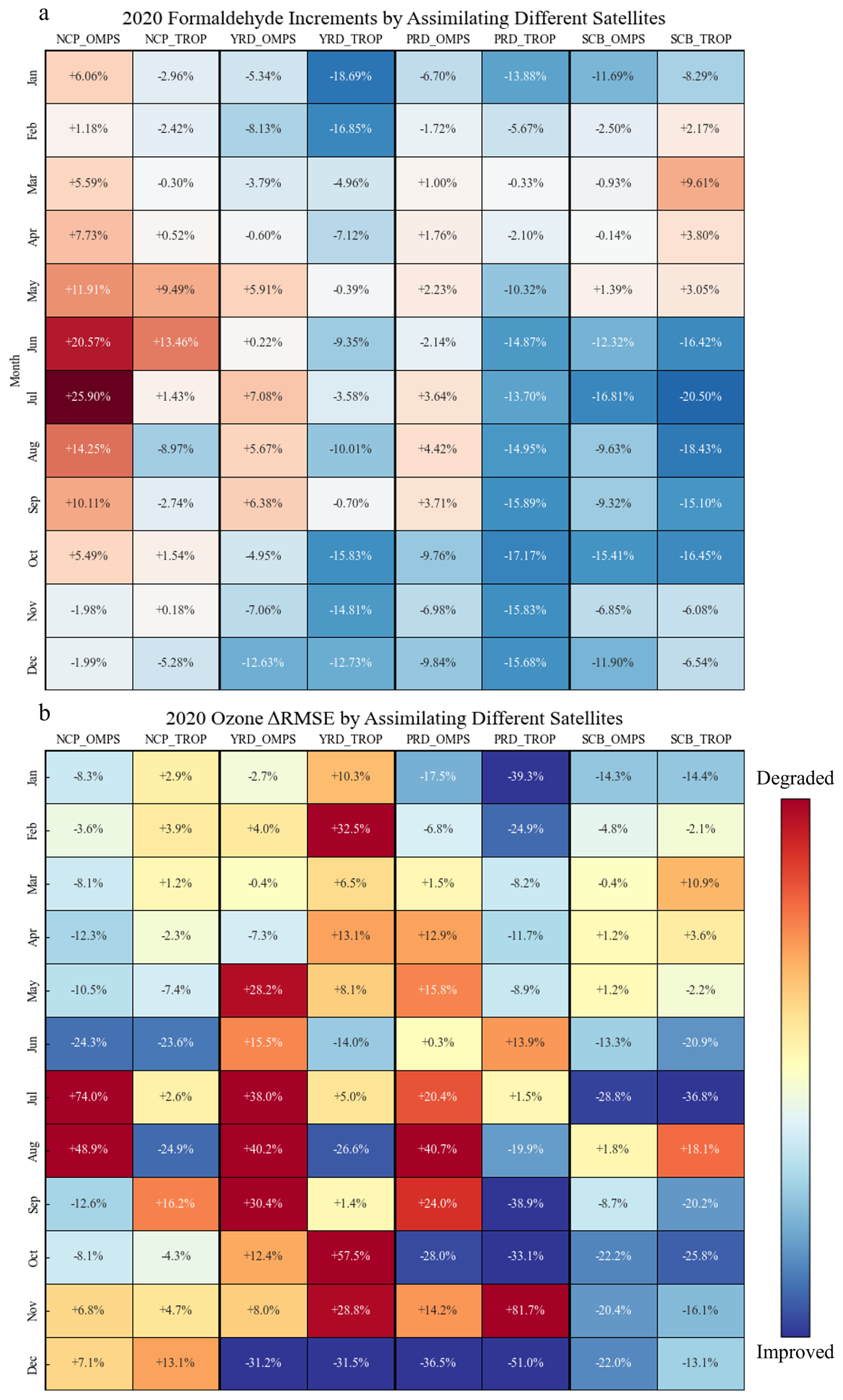
Figure 8 Monthly increments in (a) formaldehyde columns between posterior and prior simulations and (b) the relative changes in MDA8 ozone RMSE (ΔRMSE) after assimilating OMPS and TROPOMI observations in 2020. Results are shown for the North China Plain, Yangtze River Delta, Pearl River Delta, and Sichuan Basin. Positive values indicate an increase relative to the prior, while negative values indicate a decrease.

The monthly mean formaldehyde columns for 2020, derived from the prior simulation, posterior simulations constrained by the OMPS and TROPOMI observations, and satellite observations from OMPS and TROPOMI, are presented for China (a), NCP (b), YRD (c), PRD (d), and SCB (e) in Fig. 7. At the national scale, the overall changes resulting from assimilation are relatively modest, with the main adjustments occurring in summer and early autumn. The OMPS-driven posterior results show increases relative to the prior in June–July, whereas the TROPOMI-assimilated results exhibit decreases in July–August compared to the prior. These discrepancies may be attributed to differences between the satellite products in their responses to biogenic emissions and photochemical processes under high-temperature and high-radiation conditions (De Smedt et al., 2018; Vigouroux et al., 2020).

Figure 8a presents the increments between the posterior and prior simulations over the four regions when assimilating OMPS or TROPOMI observations, respectively. In the NCP, the posterior results constrained by both OMPS and TROPOMI show consistent increases in May–June, suggesting that the prior inventory may have underestimated the contributions from active photochemical production and anthropogenic emissions during summer (Wells et al., 2020). In the YRD and PRD, stronger consistency is observed in the cold season (January–March and October–December), with both posterior results showing decreases, which is consistent with reduced anthropogenic activity and lower formaldehyde production rates under wintertime conditions. The SCB exhibits more distinct characteristics, with OMPS and TROPOMI assimilation results consistently showing decreases in the second half of the year, particularly pronounced in June, July, and October. This pattern suggests that the prior emissions in this region were overestimated. Previous studies have highlighted that the large uncertainties in biogenic emissions in the SCB are critical factors influencing the accuracy of NMVOC emissions and simulations (Ma et al., 2019).

3.4 Impact of formaldehyde assimilation on ozone surface concentration

The spatial distributions of observed MDA8 ozone at ground stations (a.1–a.4), together with the prior (b.1–b.4) and posterior simulations based on OMPS and TROPOMI assimilation (c.1–c.4, d.1–d.4), are shown in Fig. 9. As shown in panels (b.1–b.4), pronounced ozone hotspots are observed in NCP (February, May, and August), YRD (May and August), PRD (May, August, and November), and SCB (May and August). This is very similar to the observations shown in panels (a.1–a.4). It indicates that the prior simulation captures the general patterns of ozone hotspots reasonably well, but notable biases remain. For example, ozone is clearly overestimated in PRD during February, May, and August, while underestimated in SCB during May and August. After assimilation with OMPS or TROPOMI, the posterior MDA8 ozone simulations retain the overall hotspot distribution, but the direction and magnitude of changes vary by region. For instance, in August, ozone concentrations increase in NCP and PRD with OMPS assimilation but decrease with TROPOMI assimilation. In February, both assimilation results decrease in YRD, although the decrease is more pronounced in the TROPOMI-based results. Moreover, many regional changes are difficult to discern visually from the spatial maps alone, highlighting the necessity of using statistical metrics to quantitatively assess ozone variations.

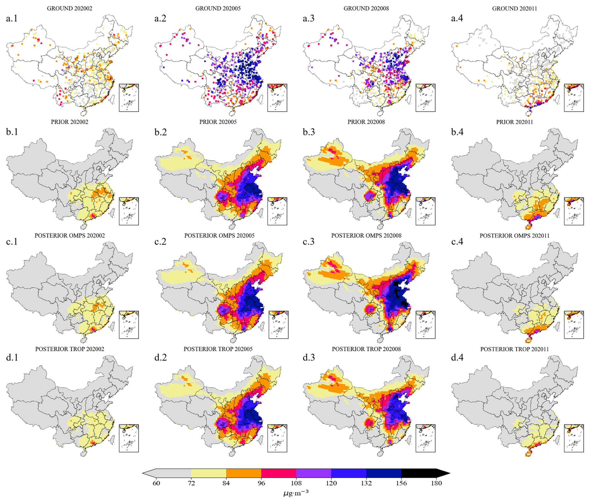
Figure 9 Spatial distributions of surface ozone concentrations in February, May, August, and November 2020. Panels (a.1)–(a.4) show ground-based observations, panels (b.1)–(b.4) show prior simulations, panels (c.1)–(c.4) show posterior simulations constrained by assimilating OMPS formaldehyde observations, and panels (d.1)–(d.4) show posterior simulations constrained by assimilating TROPOMI formaldehyde observations.

The RMSE values between the simulated MDA8 ozone and the ground-based observations are calculated. To better visualize the assimilation benefits, the RMSE variation either assimilating the TROPOMI or assimilating the OMPS in the four key regions are also shown in Fig. 8b. Larger decreases in RMSE (darker blue) indicate more significant improvements, with the posterior ozone being closer to ground-based observations; conversely, larger increases in RMSE (darker red) indicate degraded performance, with the posterior ozone diverging further from the observations. In those inconsistent cases where the OMPS and TROPOMI posterior increments exhibit opposite signs (i.e., one increases while the other decreases), ozone simulation improvement is not guaranteed. For instance, in NCP during January-April and July, in YRD during June and September, and in PRD during April, May, August, and September, one assimilation leads to improvement while the other indicates deterioration. Moreover, in several additional months both posteriors even show degradation, making it difficult to effectively evaluate the improvement in posterior ozone simulations. By contrast, ozone simulation improvements are clearly observed in consistent cases where the OMPS- and TROPOMI-constrained posteriors exhibit the same sign (i.e., both reductions in ΔRMSE). In NCP, substantial improvements are observed in May and June, with the largest RMSE decrease in June, in agreement with the high-consistency pattern shown in Fig. 8a. In YRD and PRD, RMSE decreases by more than 30 % in December, representing the most significant improvement; in addition, PRD also shows clear improvements in January and October. These improvement months all correspond to periods of high consistency. In SCB, RMSE also decreases markedly during high-consistency months, including January, June, July, and September–December.

To further quantify ozone simulation improvements in consistent regions, statistics were performed for the months classified as consistent. Considering the similarity in monthly behavior between YRD and PRD, the two regions were combined in the analysis. The results indicate that the consistent regions include NCP in May–June, YRD/PRD in January–March and October–December, and SCB in January and June–December. Within these regions, except for March and November in YRD/PRD and August in SCB, all other months show ozone simulation improvements. Overall, 13 out of the 16 consistent months exhibit improvements, accounting for 81.25 %, with an average RMSE reduction of 24.7 %. This result suggests that constraining NMVOC emissions through formaldehyde assimilation not only substantially improves formaldehyde simulations, but also exerts a positive impact on ozone simulations, with particularly significant improvements in regions and months characterized by high consistency.

To more robustly substantiate this conclusion, it is necessary to examine whether similar features can also be identified in 2019. In that year, OMPS and TROPOMI satellite observations were assimilated independently to constrain NMVOC emissions. The posterior-prior increments from the OMPS- and TROPOMI-driven assimilations, together with the changes in MDA8 ozone ΔRMSE, are presented in Fig. S6 of the Supplement. In NCP, March, May, and June are identified as consistent months, during which the ozone RMSE values decrease, with the most pronounced improvement occurring in June. In YRD, the consistent months are February, October, and November, where the ozone improvements are relatively limited but nevertheless show better agreement with ground-based observations. In PRD, the consistent months include January, February, and June–December; with the exception of August, September, and November, the ozone RMSE decreases in the other months, with notable improvements in June and July. In SCB, the two posterior datasets exhibit the highest level of consistency in 2019, with synchronous increases and decreases throughout the year. Ozone simulations in this region show better performance in all months except March and April, with particularly large improvements in June, July, and September–November, when the RMSE decreases by an average of 25.74 %.

Across the four regions, 27 months are classified as consistent in 2019. Of these, 22 months exhibit improved ozone simulations, which corresponds to 81.48 % of all consistent months, with both assimilations producing MDA8 ozone values closer to ground-based observations. This proportion differs from that of 2020 by only 0.23 %, providing further evidence that ozone improvements are particularly significant in the months defined as consistent across the four regions.

4 Summary and conclusion

In this study, satellite-based formaldehyde retrievals from OMPS and TROPOMI were assimilated to constrain NMVOC emissions over China in 2020. The results demonstrate that assimilation corrects systematic biases in prior emission inventories and improves the simulation of formaldehyde columns and surface ozone in general. More importantly, by analyzing the consistency of posterior results via assimilating different formaldehyde products across regions and months, this work establishes a methodological framework to further assess the reliability of emission estimates with multiple satellite constraints.

At the national scale, the OMPS- and TROPOMI-constrained posterior NMVOC emissions are broadly consistent across most months, with decreases in January–February and October–December and increases in March-May. The winter–spring decreases likely reflect overestimation of heating emissions in the prior inventory under reduced heating demand, whereas the spring increases are attributable to enhanced biogenic activity with rising temperatures. By contrast, notable discrepancies emerge in June–September – dominated by July–August – likely linked to strong convection, high humidity, and elevated cloud/aerosol loading that differentially affect retrievals. These discrepancies result in annual totals of 40.82 Tg (OMPS) and 34.83 Tg (TROPOMI), compared with 39.26 Tg in the prior. Regionally, NCP indicates prior underestimation in May–June consistently but pronounced divergences in July–September; YRD and PRD show warm-season inconsistencies but consistent cold-season decreases, suggesting wintertime overestimation in the prior inventory; SCB features substantial summer decreases (exceeding 20 %, particularly in June–July) alongside consistent winter decreases, while several spring months also point to possible prior overestimation.

Both the prior and the posterior simulations capture the spatial distribution of the formaldehyde columns well. When comparing the prior simulation and the posterior simulation constrained by OMPS with TROPOMI satellite observations, the prior already shows strong correlations, but further improvements are achieved after OMPS assimilation. The R² increases from 0.870 to 0.897 at the national scale and from 0.774 to 0.812 in NCP; in YRD, the increase is larger, from 0.882 to 0.918; while the largest improvements are observed in PRD and SCB, with increases of about 0.05. Meanwhile, RMSE and MAE decrease in all regions except NCP. In NCP, the simulations improve in the low-to-middle value ranges, but overestimations remain in the high-value range, likely due to the large uncertainties introduced by OMPS instrumental errors.

For ozone, comparison with surface MDA8 observations highlights significant improvements in high-consistency regions. In NCP, RMSE reductions are most pronounced in June, consistent with the strong emission and formaldehyde adjustments in this period. In YRD and PRD, December RMSE reductions exceed 30 %, while additional improvements are found in PRD during January and October. In SCB, assimilation leads to persistent improvements from January through December, with notable reductions in June–July and the late autumn months. Overall, ozone improvements are observed in 13 of the 16 consistent months, which represent 81.25 % of the total, with an average RMSE reduction of 24.7 %.

To further test the robustness of our approach, OMPS and TROPOMI satellite observations were independently assimilated to constrain NMVOC emissions for 2019 (Fig. S4). The spatial distribution of formaldehyde hotspots is similar to 2020 but with overall higher formaldehyde columns. At the regional scale, most consistent months between OMPS- and TROPOMI-constrained results indicate that the prior inventory underestimates emissions in NCP and overestimates them in YRD, PRD, and SCB. Importantly, 22 of the 27 consistent months (81.48 %) show reduced ozone RMSE, with the largest improvements in SCB, confirming that consistent cases are strongly associated with enhanced ozone simulation performance. These findings also lend greater confidence to the optimized NMVOC emissions during the consistent months in these regions.

Future efforts should reassess assimilation performance with updated emission inventories and incorporate source-specific uncertainties, assigning different uncertainties to anthropogenic, biogenic, and biomass burning sectors, in order to better constrain their respective emissions. Moreover, because no independent validation data such as aircraft or FTIR measurements were available over China in 2020, future studies could further evaluate the assimilation results once such observational datasets become accessible.