Quantifying the driving factors of particulate matter variabilities in the Beijing-Tianjin-Hebei and Yangtze River Delta regions from 2015 to 2022 by machine learning approach

Accurately quantifying the relative roles of anthropogenic emissions and meteorological conditions is essential for understanding long term changes in particulate matter (PM). Using ground observations from 40 cities, GEOS-FP meteorology, CEDS emissions, and monthly LightGBM models, this study assesses the drivers of PM_2.5 and PM₁₀ across the Beijing–Tianjin–Hebei (BTH) and Yangtze River Delta (YRD) regions during 2015–2022. The models demonstrate strong predictive skill ($R/R^{\mathrm{2}}=\mathrm{0.82}/\mathrm{0.67}$ for PM_2.5 and 0.81$/$0.65 for PM₁₀), with consistently high performance across cities. Both pollutants exhibit significant decreasing trends over the study period. Counterfactual experiments show that emission reductions overwhelmingly dominate these improvements. PM_2.5 emission driven changes intensify from −9.1 µg m⁻³ in 2016 to −31.4 µg m⁻³ in 2022, while PM₁₀ reductions strengthen from −9.8 to −42.9 µg m⁻³. Meteorology driven contributions appear as positive net anomalies at the interannual scale (approximately +2–4 µg m⁻³ for PM_2.5 and +0.5–3 µg m⁻³ for PM₁₀), indicating that air quality improvements were achieved despite year to year meteorological influences. SHAP attribution highlights 2 m air temperature (T2M), humidity (QV2M), and key precursors as dominant predictors. Interaction diagnostics further indicate that meteorological conditions modulate the effectiveness of precursor emissions, without implying direct causal mechanisms. These results provide a comprehensive data driven assessment of the factors shaping PM evolution in two major urban clusters of China.

1 Introduction

Particulate matter (PM) is a significant air pollutant and is also a critical research topic in environmental science due to its diverse sources, complex chemical composition, and profound impacts on human health (Zhang et al., 2022a). Classified by aerodynamic diameter, PM_2.5 (fine particles, ≤2.5 µm) and PM₁₀ (inhalable particles, ≤10 µm) exert differential impacts on ecosystems and human health owing to their distinct physicochemical properties and environmental behaviors (World Health Organization, 2021). Fine particles (PM_2.5) penetrate deep into the lungs and cross the alveolar–blood barrier into systemic circulation, while coarser particles (PM₁₀) deposit predominantly in the upper respiratory tract (Fu et al., 2024). Chronic exposure to PM_2.5 is linked to respiratory/cardiovascular diseases, declines in lung function, and impairment of the immune system (Franklin et al., 2008; Kioumourtzoglou et al., 2016), Whereas PM₁₀ aggravates asthma, chronic obstructive pulmonary disease (COPD), and other respiratory conditions (Seaton et al., 1995). As two pivotal economic engines of China, the Beijing-Tianjin-Hebei (BTH) and Yangtze River Delta (YRD) regions, characterized by dense industrial clusters and populations, generate substantial industrial and transportation emissions, with high-intensity production and daily activities resulting in long-standing composite air pollution dominated by PM_2.5, PM₁₀, and ozone (Dai et al., 2021, 2023), posing persistent threats to human health and urban livability. Furthermore, PM pollution acidifies aquatic environments, disrupts ecosystem balance, degrades soils, and contributes to acid rain and terrestrial biosphere damage (Dominici et al., 2014; Jerrett, 2015).

To address severe air pollution problem, Chinese government implemented the Air Pollution Prevention and Control Action Plan (State Council of the People's Republic of China, 2013) and the Three-Year Action Plan for Winning the Blue Sky Defense Battle (State Council of the People's Republic of China, 2018). These initiatives led to substantial reductions in PM concentrations nationwide (Song et al., 2023). However, China's current Ambient Air Quality Standards (GB 3095-2012) stipulate Grade II annual mean limits of 35 µg m⁻³ for PM_2.5 and 70 µg m⁻³ for PM₁₀, which significantly exceed the updated WHO guidelines (World Health Organization, 2021).

The dynamics of PM are shaped by anthropogenic precursor emissions – sulfur dioxide (SO₂), nitrogen oxides (NO_x), and ammonia (NH₃) – together with meteorological factors such as temperature, humidity, precipitation, pressure, and wind (Xiao et al., 2021). In addition to these inorganic precursors, volatile organic compounds (VOCs) also play an important role in secondary aerosol formation, particularly through pathways leading to secondary organic aerosols, as recognized in numerous atmospheric chemistry studies. PM_2.5 originates predominantly from traffic and industrial emissions, combustion processes (e.g., cooking, biomass burning), and secondary formation via atmospheric oxidation to sulfate, nitrate, and organic aerosols (Zhang et al., 2015). PM₁₀ also includes coarse particles from fugitive dust (construction, agriculture) and secondary coarse-mode particulates (Wu and Huang, 2021). The SO₂, NO_x, and NH₃ in the atmosphere can be converted into secondary inorganic aerosols, which significantly regulate PM concentrations (Ding et al., 2019; Feng et al., 2021). Meteorological parameters, such as temperature, relative humidity, precipitation, pressure, and wind, critically influence PM generation, dispersion, and removal (Leung et al., 2018; Zhao et al., 2013). For instance, elevated temperatures accelerate ${\mathrm{SO}}_x/{\mathrm{NO}}_x$ oxidation rates and fine PM formation (Chen et al., 2022). High humidity promotes particle hygroscopic growth, gas-to-particle conversion (e.g., secondary organic aerosols), and wet deposition, thereby altering PM size distribution and lifetime. These PM-meteorology interactions exhibit region- and year-specific nonlinear characteristics (Shen et al., 2017), challenging conventional linear modeling approaches (Zhao et al., 2018)

Machine learning (ML), with its capacity to capture complex, nonlinear relationships, has emerged as a powerful tool for atmospheric pollution research (Yin et al., 2022b). ML enhances source apportionment accuracy through multi-source data integration (meteorological, emission, socioeconomic), high-dimensional pattern recognition, and real-time adaptive analysis, enabling identification of complex pollutant interactions (Peng et al., 2024). For PM_2.5 and PM₁₀ studies, ML facilitates quantitative disentanglement of meteorological and emission contributions, elucidates source-receptor relationships, and informs targeted mitigation strategies.

This study employs the LightGBM framework to quantify the drivers of PM_2.5 and PM₁₀ variability across the BTH and YRD regions during 2015–2022. By leveraging LightGBM's capability to model nonlinear emission–meteorology–pollution interactions and its efficiency on multi-year, multi-city datasets, the analysis aims to identify the dominant factors governing regional air-quality evolution. The structure of this paper is as follows. Section 2 introduces the datasets used in this study, including national ground-based PM observations (Sect. 2.1), GEOS-FP meteorological reanalysis fields (Sect. 2.2), and the CEDS anthropogenic emission inventory (Sect. 2.3). Section 3 describes the methodological framework. Section 3.1 presents the extraction of city-level meteorological and emission variables from gridded datasets. Section 3.2 outlines the LightGBM modeling workflow, including the feature-engineering strategy (Sect. 3.2.1), the model training and leave-one-year-out cross-validation procedure (Sect. 3.2.2), and the SHAP-based interpretation approach (Sect. 3.2.3). The interannual trend estimation method is detailed in Sect. 3.3, and the counterfactual framework used to separate meteorological and emission contributions is introduced in Sect. 3.4. Section 4 reports the main results, including the interannual evolution of PM_2.5 and PM₁₀ (Sect. 4.1), machine-learning model performance and key predictor importance (Sect. 4.2), and the quantified meteorological and emission contributions (Sect. 4.3). Section 5 provides a broader discussion of the identified driving mechanisms in the context of chemical formation pathways and emission-control policies. Finally, Sect. 6 summarizes the key findings and presents implications for future air-quality management and research.

2 Data

2.1 Observational data from national monitoring sites

The ground-level air pollutant data for the YRD and BTH regions were acquired from the China National Environmental Monitoring Center (CNEMC) network (https://www.cnemc.cn/, last access: 31 December 2022), comprising hourly measurements of PM_2.5, PM₁₀, SO₂, NO₂, CO, and O₃ concentrations from 2015 to 2022. Observations from multiple monitoring stations within the same city were averaged to derive city-level pollutant concentrations (site-specific details are provided in Table S1 and Fig. S1 in the Supplement). The monitoring network includes 80 stations in the BTH region, covering major cities and areas in Beijing, Tianjin, and Hebei Province, and 197 stations in the YRD region, spanning Shanghai, Jiangsu, Zhejiang, and adjacent provinces. To avoid ambiguity between two cities sharing the same English spelling “Taizhou”, Taizhou City in Jiangsu Province is denoted as TaizhouJS, while Taizhou City in Zhejiang Province is denoted as TaizhouZJ throughout this study.

All national monitoring stations strictly follow the Technical Specifications for Automatic Ambient Air Quality Monitoring (Ministry of Environmental Protection of China, 2013a), ensuring standardized field operation and quality control procedures. City-level PM_2.5 and PM₁₀ concentrations are released in accordance with the national reference gravimetric method (Ministry of Environmental Protection of China, 2011), which provides the calibration and traceability framework for automated particulate measurements across the monitoring network. Gaseous pollutants (SO₂, NO₂, CO, and O₃) are measured using ultraviolet fluorescence, chemiluminescence, non-dispersive infrared absorption, and ultraviolet photometric analysis, respectively, following the national specifications for continuous gaseous monitoring (Ministry of Environmental Protection of China, 2013b). These unified procedures ensure accuracy, comparability, and long-term stability of pollutant observations.

2.2 GEOS-FP meteorological data

Meteorological fields for 2015–2022 were obtained from the GEOS Forward Processing (GEOS-FP) product (http://geoschemdata.wustl.edu/ExtData/, last access: 31 December 2020) at a spatial resolution of 0.25°×0.3125°. GEOS-FP provides hourly assimilated meteorological variables with relatively high spatial and temporal resolution, enabling refined characterization of mesoscale atmospheric processes over the BTH and YRD regions. Its near–real-time data assimilation framework has been widely applied in regional atmospheric pollution and transport studies, supporting accurate representation of dynamic meteorological conditions (Yin et al., 2021b, 2022a, b). Its near–real-time data assimilation system further improves the accuracy of reanalysis-based meteorological fields and enhances representation of dynamic atmospheric processes (Sun et al., 2021a, b; Yin et al., 2019, 2020, 2021a). The meteorological parameters used in this study include total cloud fraction (CLDTOT), precipitation flux (PRECTOT), 2 m specific humidity (QV2M), 2 m air temperature (T2M), sea-level pressure (SLP), surface downward shortwave radiation (SWGDN), and 10 m zonal (U10M) and meridional (V10M) wind components.

2.3 CEDS emission inventory

Anthropogenic emission data for 2015–2022 were obtained from the Community Emissions Data System (CEDS), which provides monthly mean fluxes at a spatial resolution of 0.5°×0.5°. In this study, we use emissions of CH₂O, CO, NH₃, NO_x, SO₂, BC, OC, and paraffinic reactive primary emissions (PRPE). Emissions were further categorized into eight sectors: non-combustion agriculture, energy transformation and extraction, industrial combustion and processes, surface transportation, residential and commercial fuel use, solvents, waste treatment and disposal, and international shipping. Anthropogenic emission data for 2015–2022 were derived from the CEDS, a global inventory providing temporally resolved sector-specific emissions. The CEDS framework supports climate change projections and quantifies human-driven interactions between air pollutants and climate systems, critical for assessing health and ecosystem impacts.

3 Methodology

3.1 Emission and meteorological data extraction

City-level emission and meteorological variables were derived from gridded emission inventories and meteorological reanalysis datasets.For each city, polygon boundaries were obtained from the GADM Level-2 shapefile, and all grid cells whose centers fell within the city polygon were identified.

For emission data, which are expressed as surface fluxes (kg m⁻² s¹), the city-scale total emission E_city(t) was obtained by physical integration over all intersecting grid cells:

$$\begin{array}{}\text{(1)}& E_{\text{city}}\left(t\right)=\sum _{i,j}{F}_{ij}\left(t\right)A_{ij}{r}_{ij}\end{array}$$

where F_ij(t) is the emission flux of grid cell (i,j) at time t; A_ij is the nominal grid-cell area; and r_ij is the fractional overlap between the grid cell and the city polygon. This area-weighted integration converts surface fluxes into physically consistent city-total emissions.

For meteorological variables, which represent intensive state quantities such as near-surface temperature (T2M), specific humidity (QV2M), and wind components (U10M/V10M), city-level averages were computed as the arithmetic mean of all grid-cell centers located inside the city polygon:

$$\begin{array}{}\text{(2)}& X_{\text{city}}\left(t\right)={\displaystyle \frac{\mathrm{1}}{N}}\sum _{i,j}{X}_{ij}\left(t\right)\end{array}$$

where X_ij(t) is the variable value in cell (i,j), and N is the number of valid grid cells within the city.

This center-based averaging is computationally efficient and provides a representative estimate of the mean meteorological condition. Because the study region lies mainly in the mid-to-low latitudes of China, where grid-cell area variation with latitude is minor, this approximation introduces negligible bias compared with full area-weighted averaging.

Both extraction procedures ensure spatial consistency between emission and meteorological datasets and yield temporally continuous, city-level time series for subsequent modeling.

3.2 LightGBM modeling

Light Gradient Boosting Machine (LightGBM) is an efficient and scalable implementation of gradient boosting, extensively applied to regression, classification, and ranking tasks (Yin et al., 2021c). By using a histogram-based decision-tree algorithm, the LightGBM model drastically reduces both computation time and memory usage compared to traditional gradient-boosting methods such as XGBoost (Bian et al., 2023; Zhang et al., 2017). It supports the direct handling of categorical variables without one-hot encoding, improving efficiency when processing high-dimensional datasets. During training, LightGBM grows trees in a leaf-wise (best-first) manner, generating deeper splits along the branch that achieves the largest loss reduction.

In contrast, XGBoost and classical Gradient Boosting Decision Trees (GBDT) use a level-wise growth strategy, which provides stability but can become computationally slower for large-scale data. LightGBM also offers extensive hyperparameter controls, such as maximum tree depth, minimum data in leaf, and feature fraction, to balance model complexity and generalization (Ke et al., 2017). Due to its high predictive accuracy, efficient splitting mechanism, and robust computational capability, LightGBM has become one of the most widely used gradient-boosting frameworks in environmental modeling (Liu et al., 2023; Wang et al., 2022; Zhang et al., 2022b).

Prior to model training, all hourly emission and meteorological inputs were aggregated to monthly means, and the LightGBM models were trained on these monthly-resolved datasets. This temporal aggregation ensured that all variables shared the same temporal frequency, preventing inconsistencies between hourly and monthly features. It also matched the model input scale with the monthly trend analysis period (2015–2022), thereby avoiding time-scale mismatches between predictor variables and the evaluation framework.

The model performance was evaluated using three widely recognized regression metrics: the correlation coefficient (R), indicating the linear relationship between predicted and observed concentrations. the coefficient of determination (R²), measuring the proportion of variance in observations explained by the model; and the root-mean-square error (RMSE), representing the average magnitude of prediction errors. Higher R and R² and lower RMSE indicate stronger predictive ability.

3.2.1 Feature engineering

To ensure interpretability and reduce redundancy, all anthropogenic emissions were aggregated into a single total value for each species (e.g., NOx_total, SO2_total). Rather than treating sector-resolved emissions separately, emissions from all sectors were summed into one unified variable per pollutant. This consolidation reduces feature dimensionality, mitigates multicollinearity among sectoral components, and preserves the dominant emission signal, resulting in a more compact and interpretable model structure.

To incorporate temporal information, three seasonal descriptors were introduced: (1) a pair of harmonic terms (month_sin and month_cos) representing the cyclic annual progression; (2) a categorical season indicator to reflect broad seasonal regimes. These features provide smooth, physically meaningful representations of seasonality without imposing sharp discontinuities between months.

In addition, two derived emission indicators were constructed to characterize temporal variability and multi-scale coupling:

Seasonal difference (sdiff) represents interannual seasonal changes over a 12 month interval. For each feature x, the seasonal difference is defined as:

$$\begin{array}{}\text{(3)}& {\text{sdiff}}_t\left(x\right)=x_t-x_{t-\mathrm{12}}\end{array}$$

where x_t denotes the monthly mean value at time t.This feature highlights annual-scale variations and helps the model capture year-to-year emission variability under identical seasonal conditions.

Rolling detrended residual (detr) represents short-term deviations from a 12 month moving-mean trend. It is expressed as:

$$\begin{array}{}\text{(4)}& {\displaystyle }{\mathrm{\text{detr}}}_t\left(x\right)=x_t-{\mathit{\mu }}_t^{\left(\mathrm{12}\right)}\left(x\right)\text{(5)}& {\displaystyle }{\mathit{\mu }}_t^{\left(\mathrm{12}\right)}\left(x\right)={\displaystyle \frac{\mathrm{1}}{k_t}}\sum _{i=t-\mathrm{11}}^t{x}_i\cdot {\mathrm{1}}_{\mathit{\left\{}{x}_i\text{valid}\mathit{\right\}}},k_t\ge \mathrm{3}\end{array}$$

where ${\mathit{\mu }}_t^{\left(\mathrm{12}\right)}\left(x\right)$ is the rolling mean computed over the past 12 months, requiring at least three valid data points (k_t≥3). This feature isolates short-term fluctuations by removing low-frequency seasonal trends.

In practice, the final predictor set comprised 35 variables: eight monthly meteorological parameters, eight species-level aggregated emission totals (e.g., NOx_total, SO2_total, BC_total), three temporal descriptors (month_sin, month_cos, season), and two derived indicators (sdiff and detr) for each emission species. Pollutant concentrations and explicit calendar identifiers (year, month, date) were excluded from the input space to avoid information leakage and to ensure consistent temporal treatment. A complete list of variables used in the model is provided in Table S2.

3.2.2 Model training and cross-validation procedure

Before model fitting, all months with missing PM_2.5 or PM₁₀ observations were removed to ensure consistency between predictors and targets. The derived emission features (sdiff and detr) inherently contain missing values during their initial 12 month computation window; these were addressed using a simple mean-imputation strategy applied within each training fold. Specifically, missing entries for each feature were replaced with the corresponding feature mean computed solely from the training subset of that fold, thereby preventing temporal leakage and ensuring that imputation relied exclusively on information available before prediction.

The LightGBM model was independently trained for each city, pollutant type (PM_2.5 and PM₁₀), and cross-validation fold. A leave-one-year-out (LOGO) cross-validation scheme was adopted, whereby data from a single year were held out for testing while the remaining seven years were used for training. This process was repeated sequentially so that each year between 2015 and 2022 served once as the held-out test period. The resulting predictions thus constitute out-of-sample estimates for every year, providing a conservative and temporally robust assessment of model generalizability and avoiding within-year information leakage.

Within each outer leave-one-year-out (LOGO) evaluation split, hyperparameters were tuned using only the training years, with the held-out test year completely excluded from all tuning steps. Specifically, a randomized search was conducted on the training subset to sample 10 candidate configurations from predefined distributions, and candidates were ranked by their cross-validated negative mean squared error (MSE) computed solely within the training data. The selected hyperparameters (learning_rate, n_estimators, num_leaves, max_depth, min_child_samples, subsample, colsample_bytree, reg_alpha, and reg_lambda) were then fixed and used to refit the model on the full training subset of that outer split before generating predictions for the held-out year. This nested evaluation design ensures that both model fitting and hyperparameter selection rely exclusively on information available prior to prediction, thereby preventing temporal leakage. A consolidated summary of the optimized hyperparameter ranges is presented in Table S3.

3.2.3 SHAP interpretation analysis

To interpret the LightGBM outputs and quantify the contribution of individual predictors, the Shapley Additive explanations (SHAP) framework was applied. For each trained model, SHAP values s_i,j represent the marginal contribution of feature j to the prediction of sample i. They are derived from cooperative game theory and satisfy the local additivity principle:

$$\begin{array}{}\text{(6)}& f\left(x_i\right)=E\left[f\right(x\left)\right]+\sum _{j=\mathrm{1}}^m{s}_{i,j}\end{array}$$

where f(x_i) is the model prediction for sample i, and E[f(x)] is the expected model output over all samples.

Because this study involves multiple cities across the BTH and YRD regions, a unified regional SHAP ranking was derived by weighting each SHAP importance of city by its corresponding number of valid monthly samples. The weighted importance for feature j is defined as:

$$\begin{array}{}\text{(7)}& I_j^{\left(w\right)}={\displaystyle \frac{{\sum }_{c=\mathrm{1}}^N{I}_{j,c}{n}_c}{{\sum }_{c=\mathrm{1}}^N{n}_c}}.\end{array}$$

Here I_j,c is the SHAP-based importance of feature j in city c, and n_c is the number of valid samples for that city, N is the total number of cities.

This weighting strategy ensures that cities with longer and more complete observational records have proportionally greater influence on the regional-level interpretability.

3.3 Interannual trend analysis method

To quantify the interannual trends of PM_2.5 and PM₁₀ concentrations from 2015 to 2022, a linear regression model was employed in this study. For each city, the relationship between annual mean concentration y and year x was modeled as:

$$\begin{array}{}\text{(8)}& y={\mathit{\beta }}_{\mathrm{0}}+{\mathit{\beta }}_{\mathrm{1}}x+\mathit{ϵ}\end{array}$$

where β₀ represents the intercept (baseline concentration), and ϵ denotes the error term. The slope β₁, reflecting the annual rate of concentration change, was estimated via the ordinary least squares (OLS) method. Specifically, the parameters were optimized by minimizing the residual sum of squares (RSS):

$$\begin{array}{}\text{(9)}& \arg \underset{{\mathit{\beta }}_{\mathrm{0}},{\mathit{\beta }}_{\mathrm{1}}}{min}\sum _{i=\mathrm{1}}^n(y_i-({\mathit{\beta }}_{\mathrm{0}}+{\mathit{\beta }}_{\mathrm{1}}{x}_i){)}^{\mathrm{2}}\end{array}$$

where n is the sample size (e.g., n=6 for the period 2015–2022), x_i denotes the year, and y_i represents the corresponding annual mean concentration.

The slope β₁ was derived as:

$$\begin{array}{}\text{(10)}& {\mathit{\beta }}_{\mathrm{1}}={\displaystyle \frac{\text{Cov}(x,y)}{\text{Var}\left(x\right)}}.\end{array}$$

The sign of β₁ indicates the direction of concentration trends (negative for decreasing, positive for increasing), while its absolute value quantifies the magnitude of change.

3.4 Methodology for disentangling meteorological and emission contributions

To quantify meteorological and anthropogenic emission contributions, the trained models were applied in a parallel prediction experiment. For each year from 2016 to 2022, anthropogenic emission features were held fixed at their 2015 levels, while meteorological and temporal predictors were retained at their actual contemporaneous values. This produced a counterfactual concentration series driven solely by meteorological variability. This yielded pollutant concentrations driven solely by meteorological variations (denoted as ML_2022met for 2022). The contribution metrics related to 2015 were calculated as follows:

Meteorological contribution (ML_2022met):

$$\begin{array}{}\text{(11)}& {\text{ML}}_{\mathrm{2022}\text{met}}={\text{ML}}_{\mathrm{15}-\mathrm{22}}-{\text{ML}}_{\mathrm{2015}}.\end{array}$$

ML₁₅₋₂₂ is the non-emission condition unchanged, the emission condition is fixed as the model prediction result in 2015, and ML₂₀₁₅ is the model prediction result with unchanged meteorological and emission conditions.

Emission contribution (ML_2022emis):

$$\begin{array}{}\text{(12)}& {\text{ML}}_{\mathrm{2022}\text{emis}}=({\text{Obs}}_{\mathrm{2022}}-{\text{Obs}}_{\mathrm{2015}})-{\text{ML}}_{\mathrm{2022}\text{met}}.\end{array}$$

Obs₂₀₂₂ and Obs₂₀₁₅: Observed concentrations in 2022 and 2015, respectively.

4 Results

4.1 Interannual trends of ground-level PM_2.5 and PM₁₀

Figure 1 illustrates the interannual evolution of ground-level PM_2.5 and PM₁₀ concentrations across the BTH and YRD regions from 2015 to 2022, with corresponding annual mean spatial distributions shown in Figs. S2 and S3. Both pollutants exhibit persistent downward trajectories across nearly all cities. The monthly time series and associated OLS trend lines (Fig. S4) further confirm that these declines remain stable throughout the study period, with the most pronounced reductions occurring before 2020. Statistical diagnostics from linear regression (Table S4) indicate that most cities display significant negative trends (p<0.05), underscoring the robustness and consistency of these decreases.

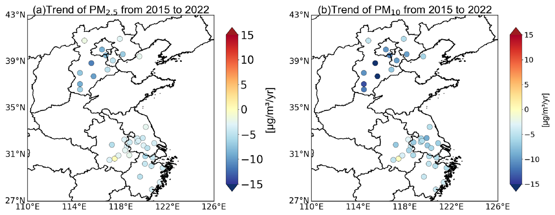
Figure 1 Interannual variation trends of PM_2.5 (a) and PM₁₀ (b) in each city during 2015–2022.

For PM_2.5, all cities show negative trends, with annual rates ranging from approximately −1.53 to −9.46 $\mathrm{\mu }\mathrm{g}{\mathrm{m}}^{-\mathrm{3}}{\mathrm{yr}}^{-\mathrm{1}}$. Within BTH, the most rapid declines occur in Baoding ($-\mathrm{9.46}\pm \mathrm{0.74}$ $\mathrm{\mu }\mathrm{g}{\mathrm{m}}^{-\mathrm{3}}{\mathrm{yr}}^{-\mathrm{1}}$), Hengshui ($-\mathrm{8.36}\pm \mathrm{0.67}$ $\mathrm{\mu }\mathrm{g}{\mathrm{m}}^{-\mathrm{3}}{\mathrm{yr}}^{-\mathrm{1}}$), and Xingtai ($-\mathrm{8.02}\pm \mathrm{0.56}$ $\mathrm{\mu }\mathrm{g}{\mathrm{m}}^{-\mathrm{3}}{\mathrm{yr}}^{-\mathrm{1}}$), while Chengde ($-\mathrm{1.98}\pm \mathrm{0.35}$ $\mathrm{\mu }\mathrm{g}{\mathrm{m}}^{-\mathrm{3}}{\mathrm{yr}}^{-\mathrm{1}}$) and Zhangjiakou ($-\mathrm{2.00}\pm \mathrm{0.42}$ $\mathrm{\mu }\mathrm{g}{\mathrm{m}}^{-\mathrm{3}}{\mathrm{yr}}^{-\mathrm{1}}$) exhibit more modest declines. In the YRD region, substantial decreases are observed in Huzhou ($-\mathrm{5.69}\pm \mathrm{1.22}$ $\mathrm{\mu }\mathrm{g}{\mathrm{m}}^{-\mathrm{3}}{\mathrm{yr}}^{-\mathrm{1}}$), Hefei ($-\mathrm{4.83}\pm \mathrm{0.33}$ $\mathrm{\mu }\mathrm{g}{\mathrm{m}}^{-\mathrm{3}}{\mathrm{yr}}^{-\mathrm{1}}$), and Chuzhou ($-\mathrm{4.28}\pm \mathrm{1.12}$ $\mathrm{\mu }\mathrm{g}{\mathrm{m}}^{-\mathrm{3}}{\mathrm{yr}}^{-\mathrm{1}}$), whereas Zhoushan ($-\mathrm{2.11}\pm \mathrm{0.14}$ $\mathrm{\mu }\mathrm{g}{\mathrm{m}}^{-\mathrm{3}}{\mathrm{yr}}^{-\mathrm{1}}$) and Taizhou-ZJ ($-\mathrm{2.72}\pm \mathrm{0.26}$ $\mathrm{\mu }\mathrm{g}{\mathrm{m}}^{-\mathrm{3}}{\mathrm{yr}}^{-\mathrm{1}}$) experience comparatively smaller reductions. These regional contrasts closely align with the initial concentration levels shown in Fig. S2, where inland BTH cities began with substantially higher baselines (e.g., Baoding and Hengshui exceeded 105 and 98 µg m⁻³ in 2015), enabling larger absolute declines.

For PM₁₀, all cities also exhibit significant decreases, with annual trends ranging from roughly −1.84 to −13.79 $\mathrm{\mu }\mathrm{g}{\mathrm{m}}^{-\mathrm{3}}{\mathrm{yr}}^{-\mathrm{1}}$. The largest reductions occur in BTH, particularly Hengshui ($-\mathrm{13.79}\pm \mathrm{1.82}$ $\mathrm{\mu }\mathrm{g}{\mathrm{m}}^{-\mathrm{3}}{\mathrm{yr}}^{-\mathrm{1}}$), Baoding ($-\mathrm{13.07}\pm \mathrm{1.46}$ $\mathrm{\mu }\mathrm{g}{\mathrm{m}}^{-\mathrm{3}}{\mathrm{yr}}^{-\mathrm{1}}$), and Xingtai ($-\mathrm{12.76}\pm \mathrm{1.29}$ $\mathrm{\mu }\mathrm{g}{\mathrm{m}}^{-\mathrm{3}}{\mathrm{yr}}^{-\mathrm{1}}$). In contrast, Chizhou ($-\mathrm{1.84}\pm \mathrm{2.03}$ $\mathrm{\mu }\mathrm{g}{\mathrm{m}}^{-\mathrm{3}}{\mathrm{yr}}^{-\mathrm{1}}$) and Zhoushan ($-\mathrm{2.77}\pm \mathrm{0.30}$ $\mathrm{\mu }\mathrm{g}{\mathrm{m}}^{-\mathrm{3}}{\mathrm{yr}}^{-\mathrm{1}}$) show the smallest declines, and the PM₁₀ trend in Chizhou is not statistically significant (p=0.40), consistent with its minimal decline rate. As with PM_2.5, cities starting with the highest PM₁₀ levels – such as Baoding (174.6 µg m⁻³ in 2015) and Hengshui (175.9 µg m⁻³) – exhibit the steepest reductions, whereas cities with lower initial levels (e.g., Zhoushan at ∼46.8 µg m⁻³) show correspondingly smaller absolute decreases.

Overall, both PM_2.5 and PM₁₀ decrease more rapidly in BTH than in YRD, reflecting regional differences in initial emissions, industrial structure, and the intensity of mitigation policies. The widespread statistical significance of the trends (Table S4) supports the conclusion that both regions experienced sustained and robust improvements in air quality during 2015–2022.

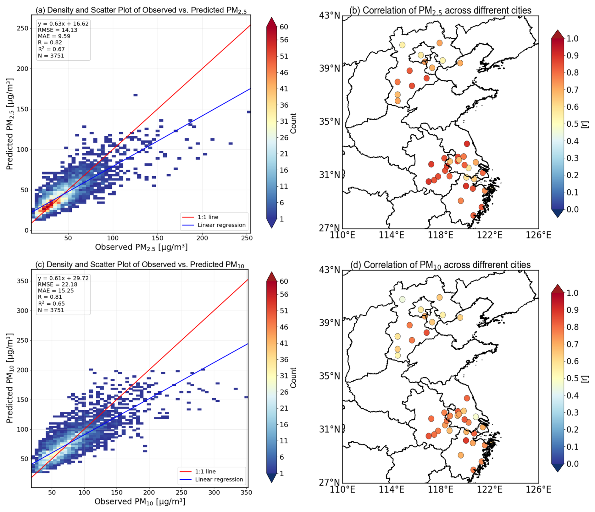
Figure 2 The density scatter plots of PM_2.5 (a) and PM₁₀ (c) concentrations observed and predicted, respectively. The correlation of PM_2.5 (b) and PM₁₀ (c) in each city over BTH and YRD regions, respectively.

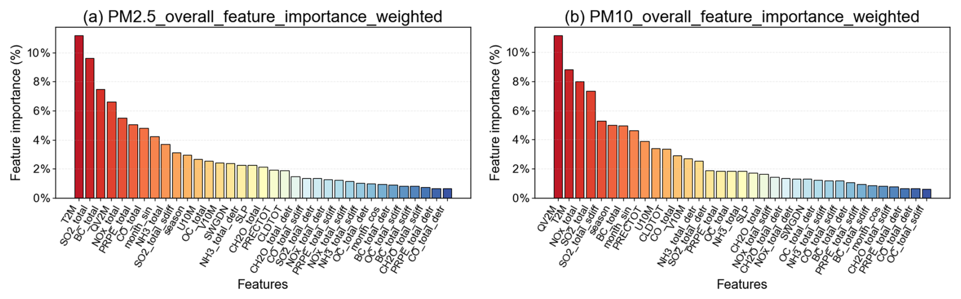
Figure 3 The feature importance of rankings of PM_2.5 (a) and PM₁₀ (b) in ML model prediction, respectively.

4.2 Machine learning model performance and variable importance

Figure 2 summarizes the predictive performance of the LightGBM models for PM_2.5 and PM₁₀ across all cities. The density scatterplots (Fig. 2a and c) show good agreement between predictions and observations, with overall $R/R^{\mathrm{2}}$ values of 0.82$/$0.67 for PM_2.5 and 0.81$/$0.65 for PM₁₀, respectively. City-level performance (Fig. 2b and d) further indicates that the majority of cities achieve correlation coefficients exceeding 0.70, as detailed in Table S5. While the predictive skill varies among cities, particularly for PM₁₀, such variability is expected given the stronger influence of coarse particle processes and regional heterogeneity. Importantly, subsequent robustness analyses (Figs. S5 and S6) confirm that this variability does not arise from model overfitting or instability, but rather reflects intrinsic differences in local PM dynamics across urban environments.

Figure 3 summarizes the SHAP-based overall feature importance. For PM_2.5, although T2M ranks as the single most influential variable in Fig. 3a, the broader pattern shows that emission-related predictors dominate the upper portion of the importance distribution, with SO2_total, BC_total, and NOx_total collectively contributing a larger share than any single meteorological factor. This implies that PM_2.5 variability during 2015–2022 remains strongly controlled by precursor emissions and their long-term reductions. In contrast, for PM₁₀ (Fig. 3b), meteorological variables, particularly QV2M and T2M, occupy the highest ranks. It should be noted that PM₁₀ inherently includes a substantial contribution from fine particles (PM_2.5). As a result, the similarity between the PM_2.5 and PM₁₀ feature importance rankings partly reflects shared driving processes affecting fine-mode particles, rather than a limitation of the modeling framework. Within this integrated metric, the elevated importance of humidity and temperature reflects their role in modulating particle mass through hygroscopic growth, boundary-layer conditions, and seasonally varying resuspension processes. Precursor emissions such as NOx_total and SO2_total remain influential, but their relative importance is reduced compared to PM_2.5.

To further assess whether the model can distinguish drivers associated with coarse particles, we additionally analyzed the coarse-mode mass defined as PM_2.5−10, calculated as PM₁₀ minus PM_2.5, using the same LOGO-based LightGBM modeling and SHAP attribution framework. The resulting feature importance rankings show systematic differences from those of PM₁₀. In particular, the dominance of humidity- and temperature-related variables and combustion-related emission proxies is reduced, whereas the relative influence of transport- and removal-related meteorological factors becomes more pronounced. Detailed results are provided in Fig. S7.

Region-specific SHAP rankings (Fig. S8) further show that PM_2.5 in the BTH region is more strongly influenced by SO2_total and BC_total, whereas the YRD exhibits greater sensitivity to meteorological conditions such as temperature and humidity. For PM₁₀, QV2M remains the dominant driver in both regions, while precursor importance (e.g., NOx_total) is consistently higher in BTH. These spatial contrasts reflect differences in emission structures and seasonal behavior between regions and underscore the need for differentiated control strategies targeting PM_2.5 and PM₁₀.

4.3 Contributions of emissions and meteorology

The spatial patterns of average emission and meteorological contributions (Fig. 4) reveal clear regional contrasts between northern cities in BTH and southern cities in YRD. For PM_2.5, emission contributions are strongly negative across most BTH cities such as Baoding, Hengshui, and Xingtai, often exceeding −30 µg m⁻³, reflecting substantial reductions from historically elevated emission levels. In contrast, YRD cities such as Suzhou, Hangzhou, and Ningbo display more moderate negative contributions, typically around −10 to −20 µg m⁻³, consistent with their lower baseline emissions. Meteorological contributions also exhibit north–south gradients: several coastal or humid subtropical YRD cities (e.g., Ningbo, Wenzhou) show slightly positive meteorological influences, whereas continental BTH cities (e.g., Beijing, Tianjin) show predominantly negative effects associated with winter stagnation, shallow boundary layers, and lower humidity. Similar spatial patterns are observed for PM₁₀ (Fig. 4b and d), where emission-driven reductions remain larger in BTH than in YRD, mirroring regional differences in emission intensity.

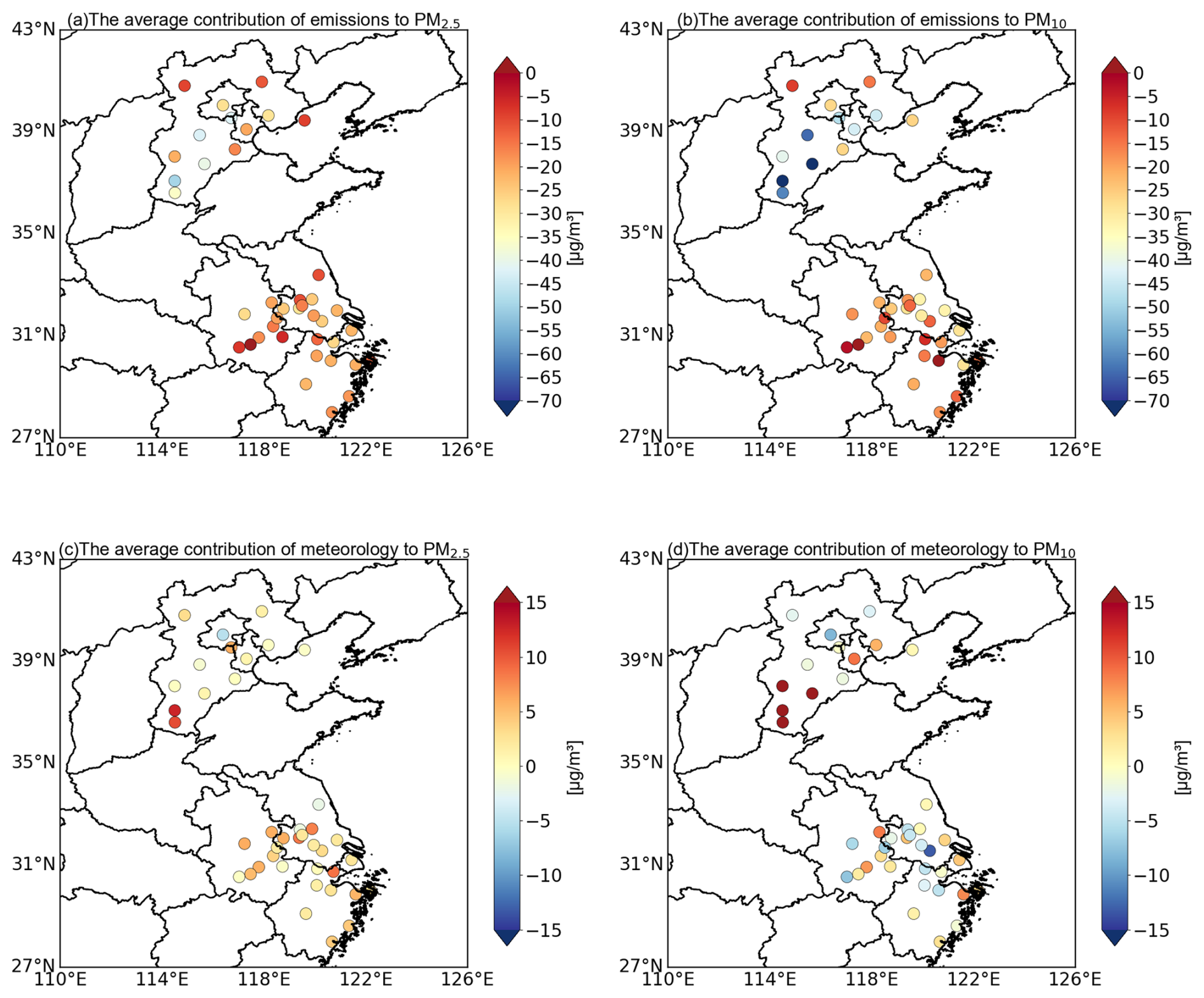
Figure 4 The average contributions of emissions and meteorological variables to PM_2.5 (for a and c) and PM₁₀ (for b and d), respectively.

The interannual evolution shown in Fig. 5 further clarifies these relationships. Emission contributions remain consistently negative from 2016 to 2022 for both pollutants and intensify over time. For PM_2.5, the reductions increase from −9.13 µg m⁻³ in 2016 to −31.39 µg m⁻³ in 2022, while PM₁₀ reductions strengthen from −9.77 to −42.91 µg m⁻³ over the same period. These progressively stronger negative contributions are consistent with sustained decreases in major emission species, including NOx_total, SO2_total, and BC_total. In contrast, meteorological contributions remain positive throughout all years, on the order of approximately 2–4 µg m⁻³ for PM_2.5 and 0.5–3 µg m⁻³ for PM₁₀, indicating that interannual meteorological conditions, on average, tended to offset part of the emission-driven reductions rather than reinforce them. Although PM₁₀ is often considered more responsive to short-term meteorological variability, the smaller meteorology-driven contributions for PM₁₀ in Fig. 5 should be interpreted in the context of interannual net effects. Meteorological influences on PM₁₀ often involve multiple processes that can act in opposite directions, such as enhanced resuspension versus enhanced dispersion and removal, leading to partial cancellation when aggregated at annual timescales. By contrast, meteorological effects on PM_2.5, particularly those related to temperature and humidity, tend to influence secondary formation and particle growth in a more directionally consistent manner at the interannual scale. This consistency allows their impacts to accumulate into a clearer net contribution. As a result, the relative magnitude of meteorology-driven changes appears larger for PM_2.5 than for PM₁₀ in Fig. 5, without implying a weaker overall meteorological sensitivity of PM₁₀.

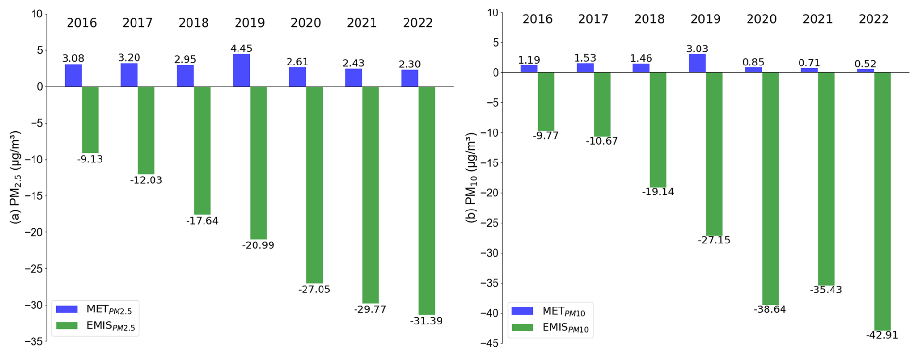
Figure 5 The averaging the emission or meteorological contributions to PM_2.5 (a) and PM₁₀ (b) of each year relative to 2015.

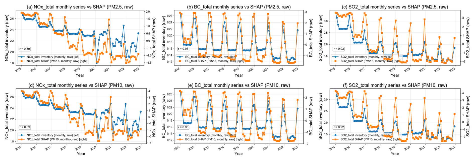
Figure 6 Monthly emission inventories of NOx_total, BC_total, and SO2_total (left y axis) and their corresponding SHAP values (right y axis) for PM_2.5 and PM₁₀ from 2015 to 2022. Panels (a)–(c) show NOx_total, BC_total, and SO2_total and their SHAP contributions to PM_2.5, while panels (d)–(f) present the corresponding relationships for PM₁₀. Emission inventories and SHAP values are plotted on separate y axes to account for their different magnitudes.

Temporal relationships between individual emission indicators and their contributions are shown in Fig. 6. For PM_2.5, month-to-month changes in NOx_total, SO2_total, and BC_total are strongly correlated with their corresponding emission-driven contributions (R=0.89–0.95). A similar correspondence is observed for PM₁₀ (R=0.89–0.93). These strong associations indicate that the estimated emission contributions respond consistently to changes in emission levels, with higher emissions generally linked to larger positive contributions and lower emissions associated with weaker contributions. This relationship persists despite the nonlinear structure of the model, which adjusts contribution magnitudes according to the prevailing meteorological conditions.

In contrast, meteorological drivers show a different temporal behavior (Fig. 7). Temperature and humidity exhibit strong negative correlations with their meteorology-driven contributions for both pollutants ($R\approx -\mathrm{0.96}$ to −0.98). Importantly, these correlations describe relative contributions at the interannual scale after emission-driven trends have been removed, rather than direct or instantaneous responses of particulate matter to meteorological forcing. At this aggregated temporal scale, years with higher temperature or moisture do not necessarily correspond to larger net meteorological contributions, because multiple meteorological influences with opposing effects can partially offset each other. These results therefore point to a scale-dependent influence of meteorology, rather than contradicting process-based studies that emphasize the role of temperature and humidity in promoting particle formation at shorter timescales.

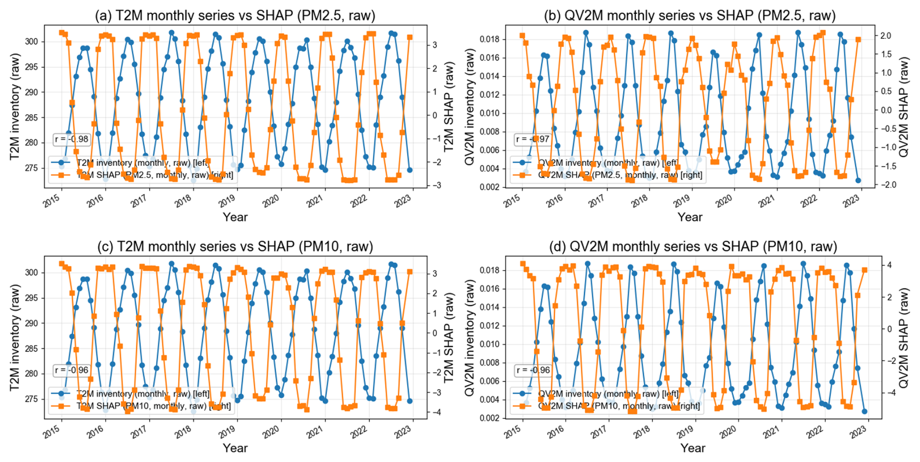
Figure 7 Monthly meteorological variables (T2M and QV2M; left y axis) and their corresponding SHAP values (right y axis) for PM_2.5 and PM₁₀ from 2015 to 2022. Panels (a) and (b) show the relationships for PM_2.5, while panels (c) and (d) present the corresponding results for PM₁₀. Separate y axes are used to account for differences in magnitude between meteorological variables and SHAP values.

Taken together, the increasingly negative emission-driven contributions shown in Fig. 5, combined with relatively modest and predominantly positive net meteorology-driven anomalies at the interannual scale, indicate that the observed improvements in PM_2.5 and PM₁₀ during 2016–2022 were mainly driven by sustained emission reductions. Meteorological conditions influenced year-to-year fluctuations but did not reverse the overall downward trends, highlighting the dominant role of emission control measures in shaping the long-term evolution of both pollutants.

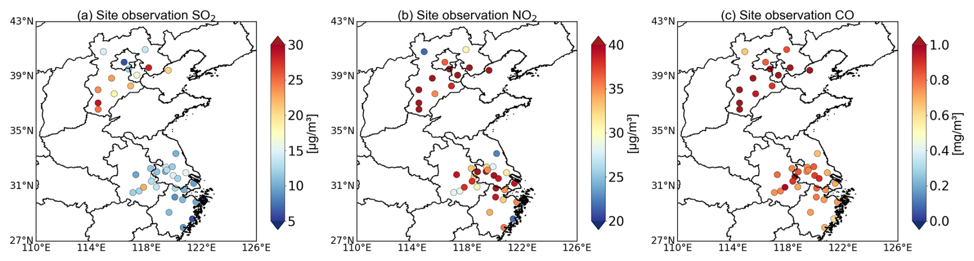
Figure 8 The average concentrations of SO₂ (a), NO₂ (b), CO (c), respectively, during 2015 to 2020 over BTH and YRD regions.

5 Discussions

To provide additional context for the SHAP-derived attributions, we examine the spatial distributions and statistical associations of key precursor species. Figure 8 shows that ambient concentrations of CO, NO₂, and SO₂ display pronounced spatial contrasts across the BTH and YRD regions. Heavy industrial cities such as Tangshan, Xingtai, Handan, and Baoding consistently exhibit higher levels of these pollutants, whereas several coastal YRD cities (e.g., Zhoushan and TaizhouZJ) show substantially lower concentrations, reflecting differences in energy structure and industrial activity. These spatial patterns offer a useful background for interpreting the correlation results summarized in Table 1.

Table 1 The correlation values among SO₂, NO₂, CO and ${\text{PM}}_{\mathrm{2.5}}/{\text{PM}}_{\mathrm{10}}$, respectively.

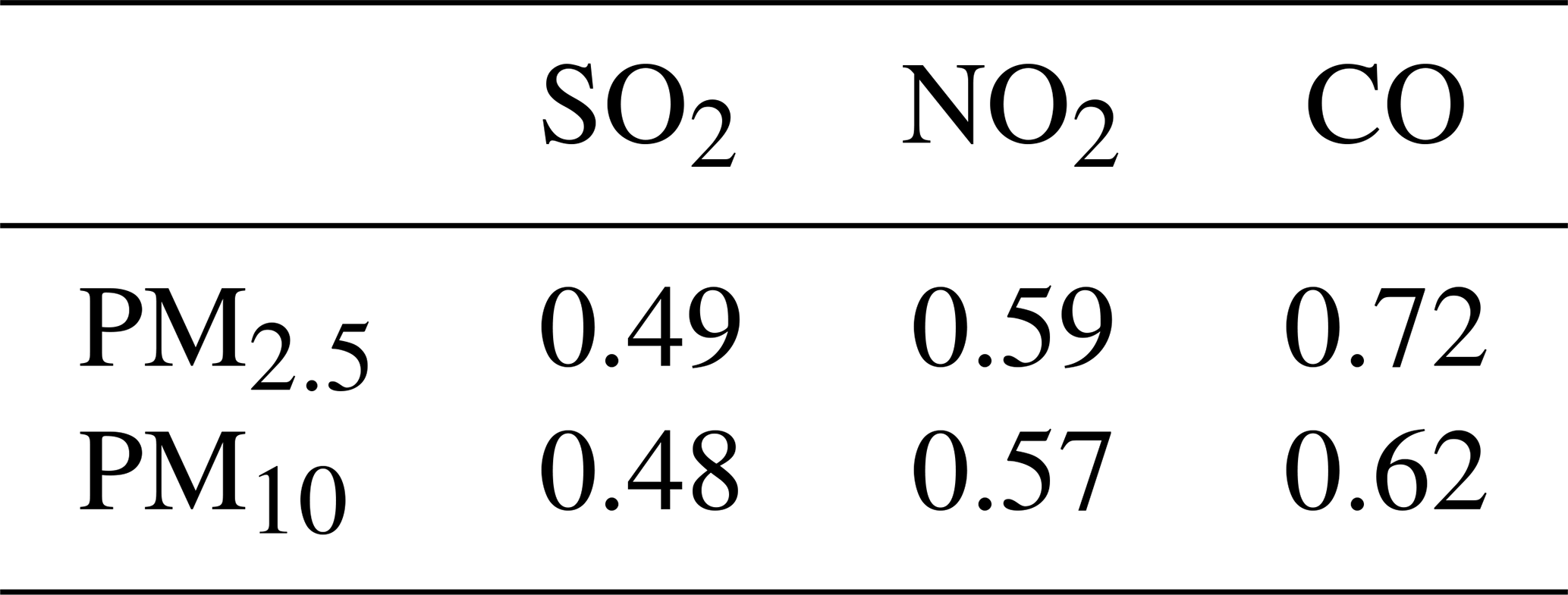
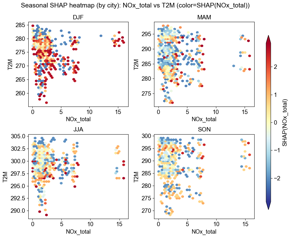
Figure 9 Seasonal scatter plots of NOx_total versus T2M across all cities, with point colors representing the SHAP contribution of NOx_total. The four panels correspond to the DJF, MAM, JJA, and SON seasons.

Across all cities, CO shows the strongest statistical association with PM_2.5 (mean R≈0.72) and PM₁₀ (mean R≈0.62), followed by NO₂ ($R\approx \mathrm{0.59}/\mathrm{0.57}$) and SO₂ ($R\approx \mathrm{0.49}/\mathrm{0.48}$). The relatively strong CO–PM relationships are consistent with their shared combustion-related origins, including traffic emissions, industrial fuel use, and residential heating, and align with recent multi-platform and top-down studies reporting tight coupling among CO, NO_x, carbonaceous aerosols, and combustion-related PM_2.5 (Tiwari et al., 2025; Wang et al., 2021, 2025). In contrast, the weaker correlations involving SO₂, despite elevated concentrations in several northern cities, likely reflect the long-term effectiveness of desulfurization policies, which have reduced sulfate formation and altered secondary aerosol composition. NO₂ correlations fall between those of CO and SO₂, indicating sustained contributions from traffic and industrial sources while also reflecting evolving chemical pathways and emission controls. Building on this context, Fig. 9 illustrates the joint dependence of NOx_total-related SHAP contributions on temperature for PM_2.5. Lower temperatures are associated with stronger NO_x-related contributions, whereas this influence weakens at higher temperatures. This pattern is consistent with established seasonal behavior in which cold conditions favor the persistence of nitrate-related particulate matter and reduced atmospheric mixing, while warmer conditions limit nitrate effectiveness and enhance dilution. Here, the interaction plot is intended as a diagnostic illustration showing how SHAP-derived contributions vary across the observed temperature range, rather than as a standalone mechanistic attribution. We do not present analogous interaction panels for PM₁₀ or for humidity-related variables. Coarse particles are more strongly influenced by mechanically driven processes such as dust resuspension and surface conditions, leading to less systematic chemical responses to temperature. Similarly, humidity affects multiple competing processes, including hygroscopic growth, aqueous-phase reactions, boundary-layer suppression, and wet removal, making it difficult to isolate a single, interpretable interaction at the seasonal scale.

Taken together, the analyses in this section are intended to complement the main SHAP-based attribution results by providing empirical context and internal consistency checks. They suggest that the statistical relationships identified by the model are broadly compatible with known emission structures, chemical regimes, and seasonal behavior, while reinforcing that the primary physical interpretation of PM variability is established by the feature importance rankings and contribution analyses discussed in earlier sections.

6 Conclusions

This study integrates multi-source emission inventories, GEOS-FP meteorological fields, and ground-based observations to investigate the drivers of PM_2.5 and PM₁₀ variability across the BTH and YRD regions during 2015–2022 using a unified LightGBM modeling and attribution framework. Both pollutants exhibit clear and statistically significant declines across most cities, supported by strong model performance under a rigorous leave-one-year-out cross-validation design ($R/R^{\mathrm{2}}=\mathrm{0.82}/\mathrm{0.67}$ for PM_2.5; 0.81$/$0.65 for PM₁₀). The consistent agreement between predictions and observations across regions and years demonstrates the robustness of the machine-learning-based representation of emission–meteorology–PM relationships at the interannual scale.

A central contribution of this work is the integration of SHAP-based interpretability diagnostics, which enables transparent attribution while retaining the flexibility of nonlinear learning. The attribution analyses indicate that anthropogenic emission reductions are the primary driver of the observed PM improvements. For PM_2.5, emission-driven decreases intensify from −9.13 µg m⁻³ in 2016 to −31.39 µg m⁻³ in 2022, while corresponding reductions for PM₁₀ strengthen from −9.77 to −42.91 µg m⁻³. These progressively larger negative contributions are consistent with sustained declines in major precursors, including NO_x, SO₂, and BC. In contrast, meteorology-driven contributions appear as comparatively smaller net anomalies at the interannual scale, indicating that year-to-year meteorological variability modulated PM levels but did not offset the long-term emission-driven downward trends.

The consistency between precursor emissions and their SHAP-derived contributions at the monthly scale, together with scale-aware temperature and humidity patterns, provides additional confidence that the attribution results are compatible with established emission structures, seasonal behavior, and chemical regimes. Rather than serving as direct mechanistic proofs, these diagnostics offer internal consistency checks that support the interpretability of the machine-learning framework.

Several methodological strengths emerge from this study. The use of harmonized monthly emission totals, multi-scale temporal descriptors (sdiff and detr), and SHAP-based interaction diagnostics facilitates a physically informed interpretation of complex emission–meteorology coupling. In addition, the explicit construction of counterfactual predictions provides a transparent approach for separating meteorological and anthropogenic influences, offering a reproducible pathway for applying machine-learning-based attribution methods to other regions and pollutants.

Despite these advantages, some limitations remain. The monthly temporal resolution cannot fully capture short-term meteorological or chemical processes; uncertainties in bottom-up emission inventories and meteorological reanalyzes may affect the absolute magnitudes of estimated contributions; and, as with all data-driven approaches, causal relationships cannot be inferred directly from statistical associations. Future work will extend this framework to explicitly examine coarse-mode particles by analyzing PM_2.5−10, enabling a clearer separation of fine particle and coarse particle drivers. Additional developments may include higher-frequency observations, expanded precursor coverage (e.g., VOCs), and hybrid machine learning and chemical transport modeling to further improve process interpretability and physical fidelity.

Overall, this study demonstrates that sustained multi-sector anthropogenic emission reductions, rather than meteorological variability, primarily explain the observed decreases in PM_2.5 and PM₁₀ from 2015 to 2022. The results highlight the value of physically informed machine learning tools, coupled with SHAP-based interpretability, for diagnosing long term air quality evolution and supporting emission control strategies grounded in observational evidence.