Ground-based observations of periodic temperature fluctuations in the mesopause region with periods longer than 2 d

We analysed more than 30 years (1988–2021) of OH^*(3,1) rotational temperatures observed from Wuppertal, Germany, with respect to periodic fluctuations (2 to 60 d) using the Lomb-Scargle periodogram. The main type of fluctuation observed in the last decades shows a period of about 28 d. Other periods which are frequently found in the observations lie in the period ranges around 2, 5 to 6, 8 to 12 d, and around 15 d and can likely be assigned to the quasi-2-day, the quasi-5-day, the quasi-10-day, and the quasi-16-day wave, respectively.

The occurrence frequency of the waves is typically higher in winter time than in summer time because of the different wave filtering in summer and winter. This winter to summer difference holds for waves with longer periods, but it breaks off in the case of shorter periods below about 20 d. The occurrence frequency of these waves with periods below 20 d exhibit two smaller maxima around the equinoxes. A further division of these observations shows that waves with periods below 10 d account for the majority of observations in the month April to September. Waves with periods between 10 and 20 d are more equally observed throughout the year except for summer.

The long-term behaviour of the wave activity indicates a quasi-bidecadal, which is likely driven by the amplitude of the waves.

1 Introduction

Planetary waves are large scale global phenomena that are known to have an important role for the global circulation due to transport and deposition of momentum for a long time (e.g. Salby, 1984; Andrews et al., 1987; Volland, 1988). They are typically generated at lower altitudes, propagate upwards, and are even able to reach the mesosphere and lower thermosphere (MLT) region under certain conditions (e.g. Holton, 1984; Laštovička, 1997; Smith, 2003; Sassi et al., 2012). Ground-based observations of wind, temperatures, and airglow in the MLT region proved as a good way to observe planetary or planetary-like waves with different periods and monitor their temporal evolution (e.g. Espy et al., 1997; Yoshida et al., 1999; Bittner et al., 2000; Luo et al., 2000; Takahashi et al., 2002; Kishore et al., 2004; Espy et al., 2005; French et al., 2005; Takahashi et al., 2005; Höppner and Bittner, 2007; Stockwell et al., 2007; López-González et al., 2009; Day and Mitchell, 2010a, b; Hecht et al., 2010; French and Kelkociuk, 2011; Takahashi et al., 2013; Egito et al., 2018; Zhao et al., 2019; Reisin, 2021). In the MLT region waves with largely different periods have been observed in the past. These periods range from only a few days in the case of very fast waves with period up to 4 d (e.g. Yoshida et al., 1999; Takahashi et al., 2005; López-González et al., 2009; Hecht et al., 2010; Egito et al., 2018; Reisin, 2021) to periods in the range of almost a week to some weeks (5 to 30 d) (e.g. Espy et al., 1997; Luo et al., 2000; French et al., 2005; Jarvis, 2006; Day and Mitchell, 2010a, b; French and Kelkociuk, 2011; Takahashi et al., 2013; Zhao et al., 2019) to periods even longer than 30 d (Espy et al., 2005; Stockwell et al., 2007; French and Kelkociuk, 2011). Some of these fluctuations at specific periods can be assigned to different Rossby wave modes. These modes are influenced by the distribution of zonal background winds and appear in the presence of such winds in rather specific period ranges such as the Rossby wave (1,4) mode at about 28 d (e.g. Kasahara, 1980; Salby, 1981a, b).

Compared to satellite observations which only observe a local point a few times a day, ground-based observations have the advantage of measuring nearly continuously. Furthermore, some ground-based instruments have been operating for several decades as the instrument can be maintained continuously which is not possible for satellite instruments. Thus, ground-based instruments and their corresponding long-time records are very suitable not only for the detection of waves but also for the analysis of the long-term evolution and the occurrence frequencies of waves with different periods. The observations by the GRIPS (GRound-based Infrared P-branch Spectrometer) instruments at Wuppertal provide one of the longest temperature time series for the mesopause region around the whole globe which has been used in several different studies (e.g. Bittner et al., 2000; Oberheide et al., 2006; Höppner and Bittner, 2007; Offermann et al., 2010; Kalicinsky et al., 2016, 2018, 2024). The observations at Wuppertal have already been used to analyse planetary waves in the past by using wavelet transform and wave proxies (Bittner et al., 2000; Höppner and Bittner, 2007). Höppner and Bittner (2007) observed a long-term periodic behaviour of the wave activity with a period of roughly 20 years similar to the Hale cycle. In their study they used the standard deviation of the temperature residuals (after subtracting the seasonal variations) as proxy for the planetary wave activity as at least a large part of these temperature fluctuations are thought to be caused by planetary or planetary-like wave activity (Bittner et al., 2000; Höppner and Bittner, 2007).

In our new study we now have the large advantage of an extended time series as Höppner and Bittner (2007) only used observations until 2005. Furthermore, we used a different technique based on the Lomb-Scargle periodogram to detect periodic fluctuations which is well suited to handle time series with data gaps (Kalicinsky et al., 2020). Compared to the previous studies this technique no longer requires data assimilation before analysis to deal with the data gaps (Bittner et al., 2000; Höppner and Bittner, 2007). The paper is structured as follows. Section 2 describes the measurements technique and the data as well as the method to detect the periodic fluctuations with some improvements made during this study. The results of the analysis with respect to the occurrence frequencies of waves with different periods and the long-term behaviour of planetary scale waves are presented in Sect. 3. These results are discussed and compared to previous results and different other observations in Sect. 4. Finally, Sect. 5 summarizes the results.

2 Measurements and data analysis

This section summarises all important information regarding the measurements and data analysis. First, the instruments and the measurement technique are described. Second, the detrending of the OH^* rotational temperatures by using a seasonal fit is explained. In the last subsection the moving Lomb Scargle method is explained. This method is used to analyse the residual temperatures with respect to periodic fluctuations in the period range between 2 and 60 d. In contrast to Kalicinsky et al. (2020), where the method is described for the first time, we improved the method in this study to overcome some of the drawbacks of the former method. These improvements are detailed in Sect. 2.3.

2.1 GRIPS instruments

The temperature observations used in this study were derived from the measurements of two GRIPS (GRound-based Infrared P-branch Spectrometer) instruments, namely GRIPS-II and GRIPS-N. GRIPS-II started its measurements in the early 1980s with temporary measurements and the continuous operation started in mid-1987. It stopped working in 2011 because of a detector failure. The GRIPS-N instrument is the follow-up instrument of GRIPS-II and continues the measurements until present (Kalicinsky et al., 2018, 2024). Both instruments were operated at Wuppertal, Germany (51° N, 7° E). GRIPS-II was a Czerny-Turner spectrometer with a Ge detector cooled by liquid nitrogen (see e.g. Bittner et al., 2002, for instrument details). The GRIPS-N instrument is also a Czerny-Turner spectrometer equipped with a thermoelectrically cooled InGaAs detector. The instrument has very similar optical properties as the GRIPS-II instrument, which makes it a suitable replacement instrument (Kalicinsky et al., 2018, 2024).

Both instruments measure three emission lines of the OH^*(3,1) band in the near infrared region (1.524–1.543 µm), namely the P₁(2), P₁(3), and P₁(4) lines. The layer of excited OH molecules is located at about 87 km height and has a layer thickness of approximately 9 km (Oberheide et al., 2006; Offermann et al., 2010). The measurements were carried out every night, except in nights with cloudy conditions. Favourable measurement conditions occur on about 220 nights per year (Oberheide et al., 2006; Offermann et al., 2010). The relative intensities of the P₁(2), P₁(3), and P₁(4) lines are used to derive rotational temperatures (see Bittner et al., 2000, and references therein). The OH^* rotational temperature may deviate from the kinetic temperature, especially in cases of higher vibrational levels. However, rotational temperatures that were determined from emissions originating from the OH^*(3,1) band are expected to be close to the kinetic temperatures (Noll et al., 2015). In addition, the analysis of periodic fluctuations does not require absolute values.

2.2 Seasonal variations of OH^* rotational temperatures

In order to analyse periodic fluctuations with periods of a few days to a few weeks one has to remove the seasonal variations first as these variations have large amplitudes and otherwise would mask the periodic fluctuations of interest. The seasonal variations can be described by an annual, a semi-annual and a ter-annual cycle (Bittner et al., 2000; Kalicinsky et al., 2024). The full description of the seasonal fit is

$$\begin{array}{}\text{(1)}& T=T_{\mathrm{0}}+\sum _{i=\mathrm{1}}^{\mathrm{3}}{A}_i\cdot \sin \left({\displaystyle \frac{\mathrm{2}\cdot \mathit{\pi }\cdot i}{\mathrm{365.25}}}\left(t+{\mathit{\varphi }}_i\right)\right),\end{array}$$

where T₀ is the annual average temperature, t is the time in days of year, and A_i, ϕ_i are the amplitudes and phases of the sinusoids. These fit parameters vary from year to year, e.g. there is a declining trend of the amplitude of the annual cycle of about −0.5 K per decade (see Kalicinsky et al., 2024, for more details). Because of these variations a fit according to Eq. (1) is used to derive residual temperatures for each year separately. One fit for the whole time series of temperatures for more than 35 years is not advisable, since the resulting residuals after subtraction of such a fit would still contain some variations (e.g. trends or year to year variations) with implications on the further analysis. The residual temperatures are analysed with a moving Lomb Scargle method and this method requires the best possible detrending of the data with respect to the seasonal variations in each year to avoid misleading results (see Sect. 2.3). Additionally, the analysis is performed such that the centre days of the time windows used always cover a complete year. To ensure that each day of a year can act as a centre day the time series used for the calculation of the residuals has to be larger than the year itself and we added two extra months at either side of the year. Then a window centred around the first and the last day of the year can be used. Another benefit of this approach is a better constrained fit at the beginning and the end of the year, since the behaviour of the observations before and after the year of interest is considered. Therefore, the new fit for the larger time interval typically compares better to a fit that is calculated for the complete winter only (fit time interval: 1 July to 30 June – of the next year) at the beginning and end of the year. This also leads to a reduction of discontinuities at the year borders compared to a fit using the data of one year only.

Figure 1 shows an example of the seasonal fit for the year 1997. The data are shown in a 16 month interval centred in summer. In addition to the seasonal fit in this time interval (red curve in Fig. 1) the fits to the data from 1 July to 30 June of the previous and following year are shown as blue curves. In the transition region from one year to the next (solid blue line in Fig. 1) the agreement between the fit for the year itself (red curve in Fig. 1) and the two fits centred in winter (solid blue line in Fig. 1) is reasonably good. The vertical dashed lines mark the time interval of 14 months which is the largest interval used in the moving Lomb Scargle method (see Sect. 2.3). The residual temperatures (data – fit) that are analysed are shown in the lower panel of Fig. 1.

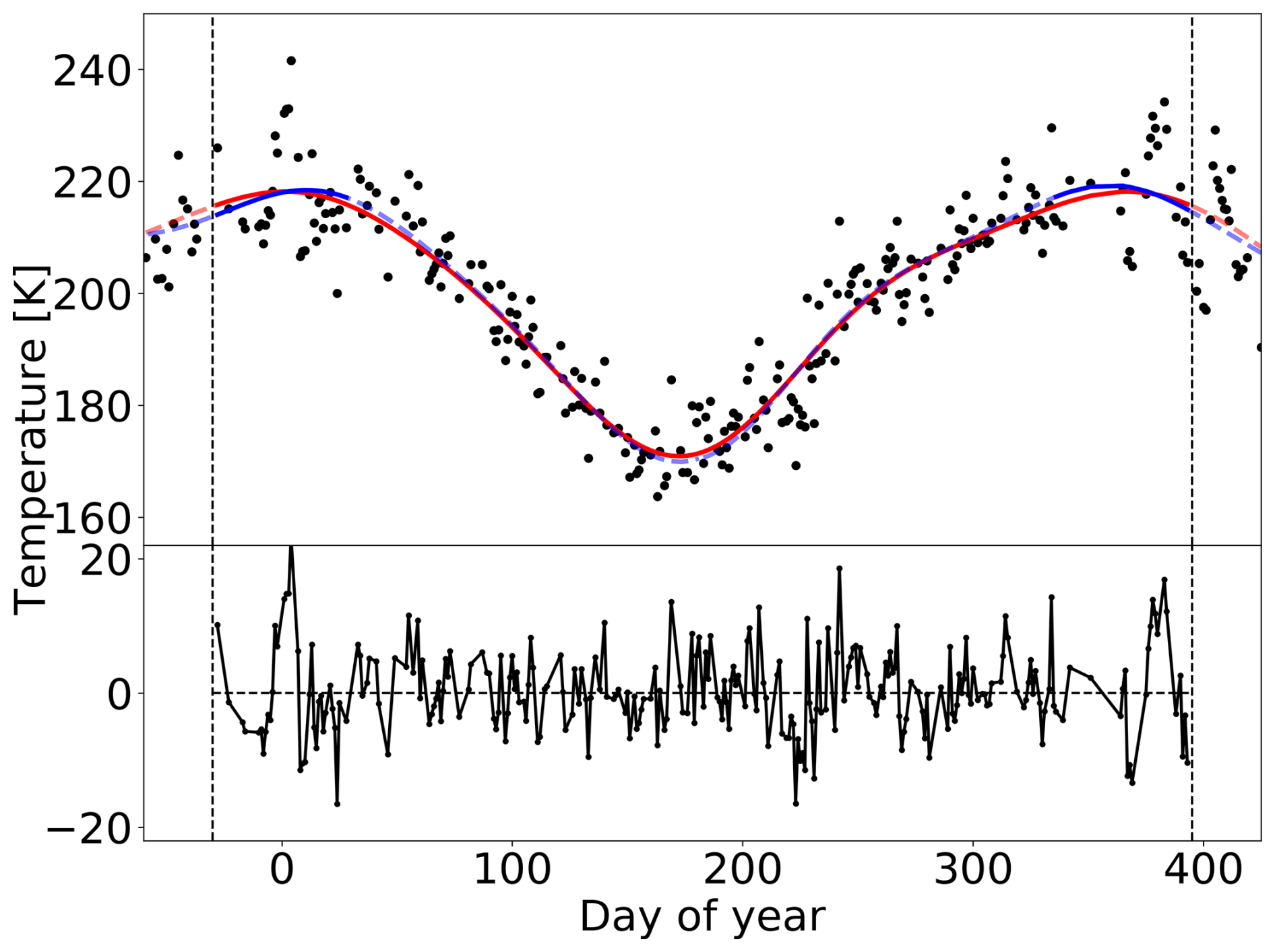
Figure 1 Seasonal variations of the OH^* rotational temperatures in the year 1997 with two months added at both sides. The black dots show the OH^* rotational temperatures and the red curve shows the fit curve according to Eq. (1) to the 16 months interval. The blue curves show the fits to the data from 1 July to 30 June of the previous and following year. The vertical dashed lines mark the 14 month interval centred in summer. In the lower panel the residual temperatures (data – fit curve) of this 14 month interval are displayed.

2.3 Moving Lomb–Scargle periodogram

The periodic fluctuations are analysed with the moving Lomb-Scargle periodogram (Kalicinsky et al., 2020). The method is based on the original Lomb-Scargle periodogram (LSP) (Lomb, 1976; Scargle, 1982). This method that can detect periodic fluctuations in all kind of time series even in time series with unequal spacing, which is the case when data gaps are present. Thus, it is very suitable to analyse OH^*(3,1) rotational temperature time series that exhibit irregular data gaps due to weather conditions. In the approach described by Kalicinsky et al. (2020) a time window of fixed length, for example 60 d, is used for the analysis. The starting point is the beginning of the time series and the window is shifted by the minimum sampling step (here 1 d) until the end of the time series is reached. For the data points within each of these individual time windows, that all include a different part of the complete time series, a LSP is calculated separately. In this way periodic fluctuations can be detected in combination with the temporal evolution of the periods and amplitudes of these fluctuations (see Kalicinsky et al., 2020, for a complete description of the method).

The use of a fixed window length has a drawback, which is mainly noticeable in the case of signals with periods much shorter than the window length. It is not very likely that such a signal with a period of only a few days remains in atmospheric temperatures for several weeks. When the time window is much longer than the duration of such an event the results using the LSP are damped, i.e. the period and amplitude is a mean value over the whole time interval. In such a case the amplitude is typically much smaller than it would be when a shorter time window would be used. As a consequence events with short periods and a small duration may be missed in the analysis. In order to avoid this drawback we introduced a varying window length here. The window length changes simultaneously to the analysed period, i.e. a smaller window is used for shorter periods and vice versa. The window length can only be reduced to a certain threshold value, because of two important points. First, the data gaps should not exceed the length of the window used. Second, the significance of the results depends on the number of data points (e.g. Cumming et al., 1999; Zechmeister and Kürster, 2009; Kalicinsky et al., 2020) which hinders the use of too small windows. The significance of a result for the same signal decreases if less data points were incorporated in the analysis, i.e. the possibility to produce such a signal by chance e.g. due to noise is larger in the case of less data points. Therefore, a signal that accounts for the same variance of the total time series could be significant if more data points were used for the analysis and not significant for less data points. In total, the minimum window length has to be a trade-off. On the one hand, it has to be large enough to avoid problems with too many data gaps and worse significance and, on the other hand, it has to be small enough to detect events with short periods and short duration. Below the threshold value the window length stays constant.

We also used the number of cycles of an oscillation at a given period as a factor to calculate the window lengths and the stepping. A factor of one means the analysed period and the time window are always the same. In the case of the factor of 2 the window length is twice as large as the period analysed using this window, i.e. two cycles of an oscillation with a certain period would fit in the time window used for the analysis. The minimum window length (divided by the factor) still defines the minimum period below which the time window stays constant. For example the scaling factor of 2 sets the minimum period to 12 d up to which the periods below are analysed with the defined window length of 25 d. After the period of 12 d the rounded double window length corresponding to the analysed period is used, e.g. 26 d for 12.6 d, 27 d for 13.2 d, 30 d for 14.9 d, 40 d for 19.9 d and 120 d for 60 d. The scaling of the minimum period has been done to ensure a softer transition to larger window lengths.

The significance of the results is analysed using the false alarm probability (FAP). The FAP gives the probability that a certain peak with a certain normalized power can occur just by chance somewhere in the whole analysed period range. It is determined using an empirical expression where the coefficients were determined by using Monte Carlo simulations. By using this expression the significance for each peak can be evaluated depending on the window length, period range and number of data points (see Kalicinsky et al., 2020, for more details). Compared to the former approach described in Kalicinsky et al. (2020) the range of window lengths is now larger, since the window length changes in relation to the analysed period. In the former evaluation of the significance in dependence of the window length only lengths of 30 d and larger have been considered. In this study we also use smaller window lengths. Therefore we reevaluated the significance in dependence of the used window length and the analysed period range in a larger range of window lengths (10 to 90 d) and for more representations. Here we simulated 100 times 10 000 representations instead of only one time 10 000 representations as done in Kalicinsky et al. (2020). In this way we obtained new results that give refined coefficients for Eq. (6) in Kalicinsky et al. (2020) with an improved estimation of the uncertainties. The new values of coefficients are 2.98±0.02 d d⁻¹ for the slope and $-\mathrm{0.23}\pm \mathrm{0.01}$ d⁻¹ for the intercept. The given uncertainties are one times the standard deviation of their mean. Thus, the new results show that the former results by Kalicinsky et al. (2020) were by chance at the end of the 3σ range for both values. Additionally, small differences may occur from the wider range used for the window lengths.

A prerequisite for the whole method is a good detrending with respect to the seasonal variations in each year. Otherwise, remaining underlying trends will influence the results. Three different problems are known to us. First, a trend can lead to a reduction of the normalized power in comparison to the same time series without trend. As a consequence the significance of the result is reduced as well because of the reduced power. This can lead to a missed event. Second, a trend can also lead to a shift of the period where the maximum power is observed. This would lead to a bias of the results. Third, in some cases for periods with a period length close to the window length the amplitude of the oscillation is overestimated as the fitted sinusoid tries to compensate also for the trend. This would lead to a wrong estimation of the amplitude. Thus, we used the fitting approach as described in Sect. 2.2 to avoid these problems.

Figure 2 shows a comparison between the new results using the varying window and the old results with a fixed window length of 60 d for the example year 2005. The values used for the analysis with varying window length are a minimum window length of 25 d and a factor of 1.0. The window length stays constant at a period of 25 d and below and monotonically increases with increasing period above this value. Obviously, the new results allow for more variability of the amplitude as the smoothing effect is smaller. Because of these lower fluctuations and higher significance levels in the case of more data points used for the analysis, it may occur that the time interval showing significant results is slightly larger in the time domain for the results with the fixed window. This effect mainly shows up at longer periods. The benefit of the new method arises at shorter periods. Thus, in the result for the improved method many more significant events are detected (see Fig. 2a). These events are typically very short in duration. In the case of a fixed window with too large size these events will be smoothed such as they are not detectable any more (see Fig. 2b). Thus, with the method described by Kalicinsky et al. (2020) significant events could be missed and the improved method presented here gives a large benefit.

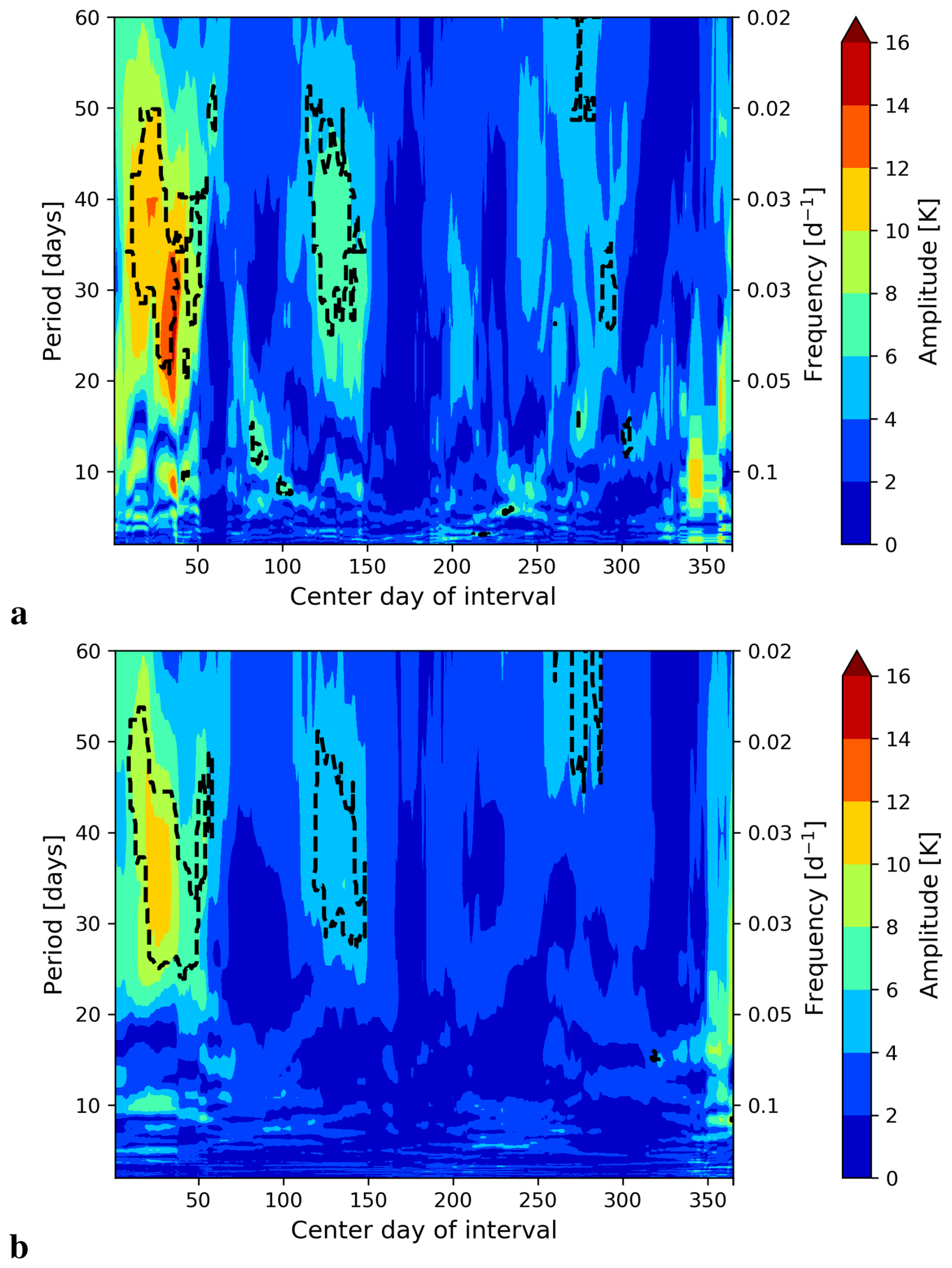
Figure 2 Comparison of the LSP results for the amplitude in the year 2005. (a) Improved method with varying time window. The minimum window length used for the analysis was 25 d, i.e. below a period of 25 d the window length was constant at 25 d an monotonically increased above this threshold period. (b) Former method with fixed window length of 60 d. The x axes show the centre days of the time windows and the y axis the period and frequency, respectively. The amplitude displayed is colour coded. The black contour lines mark the region of significant results.

3 Results

This section is divided into two parts. In Sect. 3.1 the periods of different fluctuations that are typically caused by planetary waves are analysed. This includes the occurrence frequencies of the observed periods and also seasonal differences of the occurrence frequencies for specific period ranges. Section 3.2 focuses on the long-term evolution of the wave activity, which mainly deals with the question if there is a long-term trend or even a long-term periodic behaviour of the wave activity. All presented figures were deduced from LSP results that have been calculated with the new approach with varying window length. The minimum window length was 25 d and the factor 1. Only periodic fluctuations that have been classified as significant events using the FAP and our empirical equation to calculate it (see Sect. 2.3) were taken into account, i.e. only results inside the contour lines in Fig. 2a were used.

3.1 Occurrence frequencies of waves

In the first step we simply counted the days of each individual event, i.e. all centre days that lie inside a contour line and, thus, show a significant event. As events with longer period tend to last longer, we divided the counts in each bin by the mean period of the corresponding bin. This leads to an observation frequency in terms of cycles and removes the dependency on the period. These results show the relative importance of the waves at different periods. Furthermore, it still accounts for the length of the individual events, i.e. longer events including more cycles still get a stronger weight compared to shorter events. This would not be the case if the events themselves would be counted only.

Figure 3 shows the occurrence frequency of events with certain periods. The preferred periods are about 28, 15, 12, 10, 8 d, in the period range of 5 to 6, and 2 d. Thereby, the most events were observed at periods of about 28 d. Additionally, there are numerous detections of waves with periods longer than 30 d, but here no clear maximum can be observed.

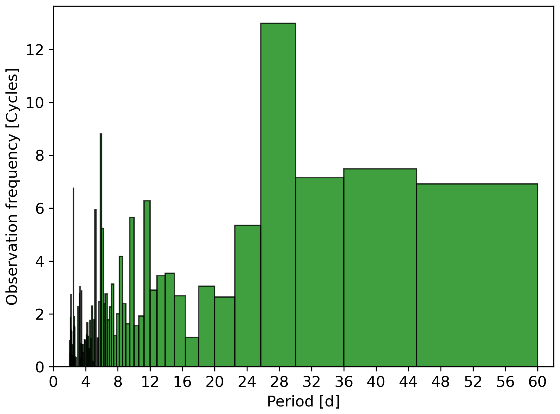
Figure 3 Occurrence frequency of events in dependency of the period. The histogram shows the number of centre days of the LSP analysis with significant results divided by the mean periods of the corresponding bins.

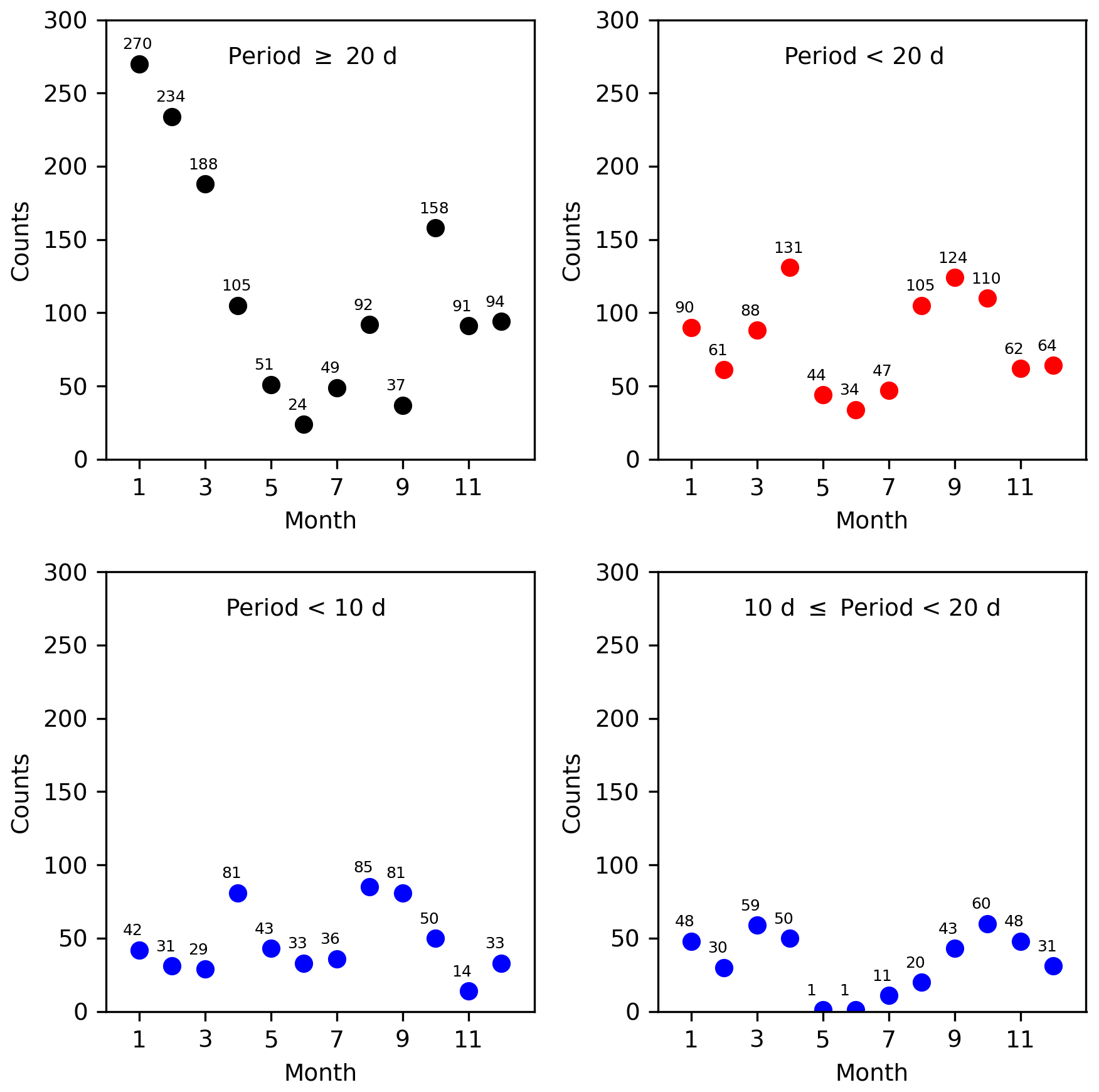
Figure 4 Seasonal dependency of the occurrence frequencies of events with different periods. In the upper panel of the figure the number of centre days with significant results are plotted against the month for the period range ≥ 20 d (left panels) and the period range < 20 d (right panels). A further subdivision of the second period range is shown in the lower panel. The results for the period range < 10 d is shown in the lower left panel and the results for the period range between 10 and 20 d is shown in the lower right panel.

The seasonal dependency of the occurrence frequencies is largely dependent on the period itself. Figure 4 shows the number of centre days with significant events plotted against the month for different period ranges. In the upper panel of Fig. 4 the period range is longer or equal to 20 d (left panels) and shorter than 20 d (right panels). Obviously, events with periods ≤ 20 d occur more often in winter time than in summer time. In this period range the largest numbers were observed in January and February and the lowest numbers in June. In the case of events with shorter periods the situation is largely different. In the period range < 20 d the largest number of events were detected around the equinoxes (late March and late September). The maximum number of days with significant events were observed in April and September. Thereby, the number of days with significant events around the equinox in fall is larger than in spring time. Note here, that this important result is only visible by using the new approach with the varying window length. When using the former approach described in Kalicinsky et al. (2020) a large number of events with shorter periods are missed and the clear seasonal structure with the maxima around the equinoxes is obscured. The lower panel of Fig. 4 shows a further subdivision of the shorter periods. The results for the period range below 10 d is show in the lower left panel and the results for the period range between 10 and 20 d is shown in the lower right panel. The contribution of events with periods below 10 d is partly very high. In the months from May to June these waves account for nearly all observations. In the months around the equinoxes (April, August, and September) the proportion of the waves with the shortest periods is still larger than 60 % and the waves with periods < 10 d still account for the majority of observations in the whole period range < 20 d. The results in the period range between 10 and 20 d do neither show clear maxima at the equinoxes nor maxima in winter. The observations are more equally distributed over the whole year with no detections in summer.

The distribution of the observed amplitudes of the events is shown in Fig. 5. Note here that all single amplitudes that correspond to centre days within an event are displayed, i.e. one event would have its own distribution of amplitudes. The mean amplitude of all events is 7.9 K with a standard deviation of 2.8 K. The smallest amplitudes that belong to a significant fluctuation are slightly above 2 K and the largest observed amplitudes are nearly 16 K. When the amplitudes are plotted for different period ranges (not shown), no obvious difference can be seen. Thus, the amplitudes are not significantly larger for events with shorter or longer periods. Note here that there might be some reduction of the amplitudes due to vertical averaging, especially for waves with shorter periods and smaller vertical wavelengths. In the majority of the cases waves with periods even below about 10 d exhibit vertical wavelengths that are a multiple of the FWHM of the OH layer (e.g. Buriti et al., 2005; Ern et al., 2013; Yamazaki and Matthias, 2019; Reisin, 2021). Very small vertical wavelengths below e.g. 20 km are only reported for a very minor portion of all observations (Reisin, 2021). Thus, the averaging effect should be small or maybe even negligible.

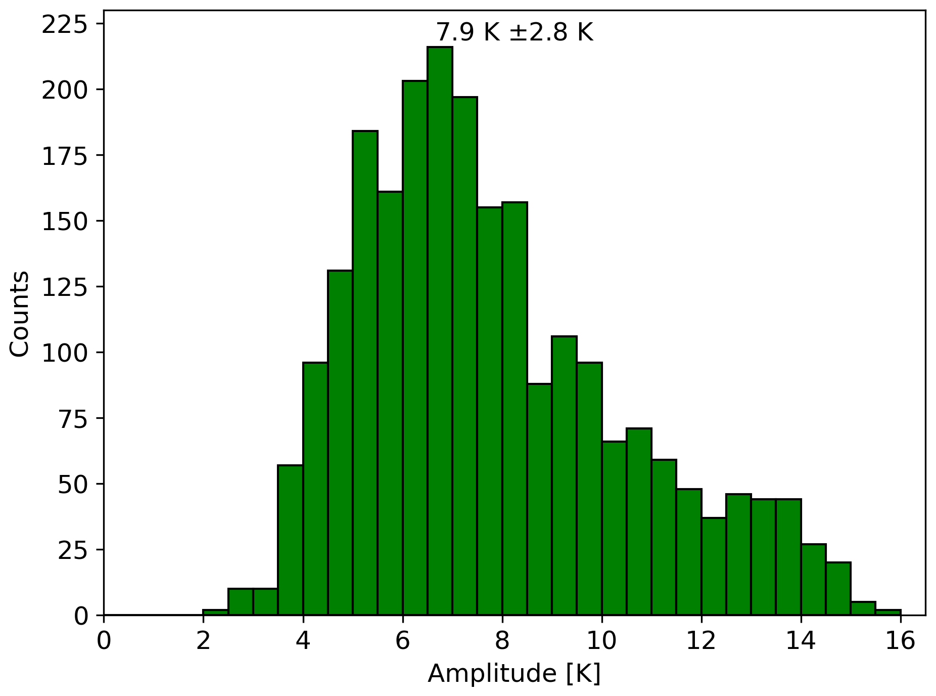
Figure 5 Distribution of the observed amplitudes. All single amplitudes that correspond to centre days within an event are displayed.

3.2 Long-term evolution of wave activity

The second part of this study deals with the long-term evolution of the wave activity. In former studies this long-term evolution was analysed by using the standard deviation of the residual temperatures (data – seasonal fit) for each single year as a proxy for the wave activity in this year (e.g. Höppner and Bittner, 2007). The authors observed a quasi-bidecadal oscillation of the wave activity in this study. The standard deviation as proxy has the drawback that all kind of fluctuations are included in this quantity and not only the significant ones. Because of this, we use the mean amplitude of the significant events as a new proxy. This new proxy also has a small drawback, because it does not include the length of the events, only the strength. Thus, we also use the amplitude weighted sum of significant days as another proxy, i.e. the mean amplitude times the number of days at which a significant event was detected. As all of the three proxies have similarities and also differences the comparison of the individual LSPs can help to gain information on the importance of the length and the strength of the wave events on certain periodic behaviours. Figure 6a shows the time series of all three different quantities (with mean subtracted). The periodicity of the time series is analysed with the LSP and the results are shown in Fig. 6b with the same colours as used in Fig. 6a. The two time series in the two upper panels in Fig. 6a, the standard deviation and the mean amplitude, show a rather similar behaviour with corresponding times of maxima and minima. Only at some points, for example in the years 2007 and  009, there are larger differences. The LSPs for these two time series show also peaks at very similar periods (see Fig. 6b). The main peak in the long-period range is located at about 20 years in both cases. The maximum in the LSP for the mean amplitude lies slightly below 20 years (red curve in Fig. 6b) and in the case of the standard deviation slightly above this value (black curve in Fig. 6b). Due to the uncertainty (the width of the peaks) this difference is not significant. These two peaks at about 20 years are not significant at a 95 % confidence level with respect to the complete analysed period range (FAP). This is a common problem with this rather conservative approach in the case when several similar large peaks occur in a periodogram, but does not mean that the oscillations are not real. With respect to the single frequency the significant level for the peak at 20 years is almost 95 % in the case of the standard deviation and better than 95 % for the mean amplitude, i.e. it is rather uncertain that a peak with that height occurs at exactly this period just by chance. As we are searching for a peak at a period of 20 years because of the former study by Höppner and Bittner (2007), this second way is valid here. The time series of the weighted sum of significant days does not show the same long periodic fluctuation as the other two quantities (lower panel of Fig. 6a and blue curve in Fig. 6b). The difference between the time series of the mean amplitude and that of the weighted sum is simply the number of days with significant results. Consequently, the fact that only one time series shows the long-term oscillation implies that only the amplitude of the events shows these long-periodic behaviour and not the number of days. As the standard deviation is a measure of the amplitudes of all fluctuations within the analysed time interval, the standard deviation shows almost the same long-term behaviour. Furthermore, this also indicates that in most years the significant fluctuations dominate the standard deviation of the residual temperatures.

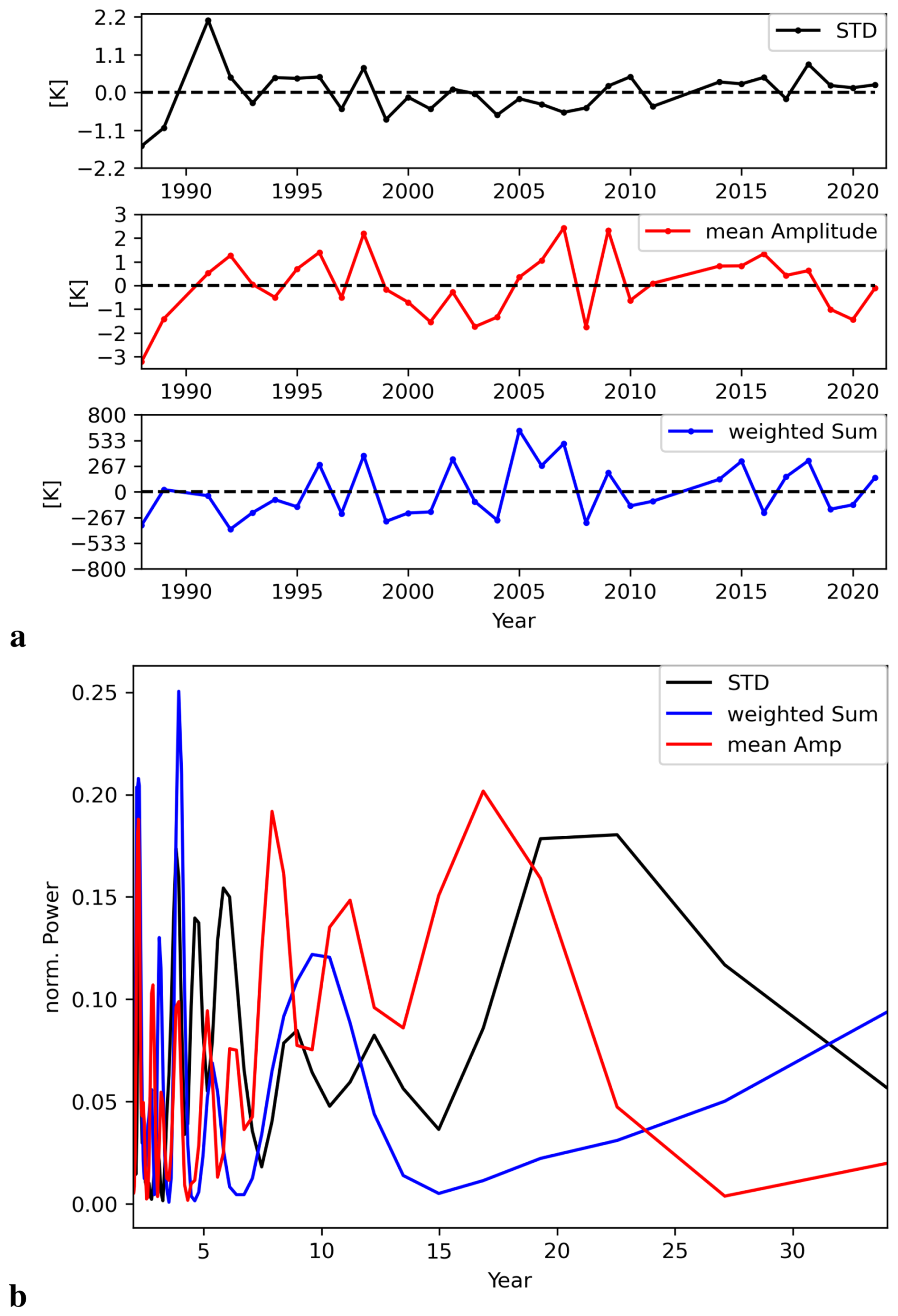
Figure 6 Long-term behaviour of the wave activity. (a) The upper panel shows the time series of the yearly standard deviation of the temperature residuals after subtracting the seasonal fit. In the middle panel the time series of the mean amplitude of all significant events in a single year is displayed. The lower panel shows the product of the mean amplitude and the sum of the centre days with a significant result in the LSP. (b) The LSP for the three time series are shown with the same colours as of the time series themselves (black: standard deviation, blue: weighted sum, red: mean amplitude).

The peak that has the largest power in all of the periodograms is the peak at about 4 years in the LSP of the weighted sum of days. As before the peak is not significant with respect to the complete period range but highly significant with respect to the single frequency. A fit to the time series gives a period of nearly exactly 4 years. As only one proxy shows a clear peak, we do not further interpret the results.

4 Discussion

The discussion is divided into two parts. First, the observed fluctuations are compared to other results and the seasonality of the wave occurrence is examined. In the second part, the long-term behaviour of the wave activity and the fluctuation of this activity itself is discussed.

4.1 Periodic fluctuations

The highest peak in the histogram occurs at a period of around 28 d (about 25 to 30 d in Fig. 3). This shows that period fluctuations in this period range are very common. Waves in this period range are observed at the largest number of days (not shown) as well as for the largest number of cycles. Thus, these waves are the most important ones in relative and absolute terms. And indeed, in a larger number of winters an event with an average period in this range takes place. Figure 7 shows an example for such an event. The time series of the temperature residuals over the winter 1997/1998 is shown as black curve in Fig. 7a. Obviously, between the days 160 and 260 a large periodic fluctuation is present. The amplitude of this fluctuation increases at the beginning and reaches maximum values around day 215. Then it decreases again. The red curve shows a sinusoid with varying amplitude fitted to the data. The resulting mean amplitude is about 26 d and, thus, falls in the period range from about 25 to 30 d. The LSP results in Fig. 7b shows some deviation from this mean period at the beginning of the event, where the period of the maximum peak in the LSP lies slightly above 30 d, but only for a few days. Therefore, we would still categorize the whole event as a quasi-28 d wave. A very similar event was observed over Antarctica at Rothera station in the winter 2014 (Zhao et al., 2019). The authors used ground-based and satellite data to analyse the vertical and horizontal structure of this event and find that it was consistent with the Rossby wave (1,4) mode. This is also consistent with theory where the Rossby wave (1,4) mode has a period of about 28 d in the presence of zonal background winds (Kasahara, 1980). Zhao et al. (2019) state in their study that the propagation in the MLT region is severely limited in summer because of the low phase speed of this type of waves. They also refer to a study by Sassi et al. (2012) who found that the propagation to higher altitudes is expected to be transient because of the effect of the background winds and the wind filtering. This could also explain that we observe the 28 d wave typically in winter and not in summer. There is another possible effect on the temperature in the mesopause region that shows a periodic behaviour in the same period range: the 27 d solar cycle. But the known amplitudes of this influence are considerably smaller than the ones observed here. Beig et al. (2008) reviewed studies concerning the influence of the 27 d solar cycle on temperatures in the mesosphere and lower thermosphere and reported values less than 4 K. Typically the values in the mesopause region are smaller than in the mesosphere itself. Other studies also show periodic fluctuations in coincidence with the 27 d solar cycle (a time-lag is present) with amplitudes smaller than 1 K (von Savigny et al., 2012; Thomas et al., 2015; Rong et al., 2020). Thus, the amplitudes of the fluctuations observed here are much larger than what is expected in the case of the 27 d solar cycle. We also analysed the GRIPS OH(3,1) rotational temperatures with respect to the influence of the 27 d solar cycle and observed similar amplitudes (<1 K) than in previous studies. Furthermore, we excluded time intervals in winter with strong events in the 27 d period range from the analysis and observed no significant differences to the previous results (Christian v. Savigny, personal communication, 2025). This led us to the conclusion that the influence of the 27 d solar cycle on the temperatures and the fluctuation with periods of about 28 d that partly show amplitudes greater than 10 K are two completely independent phenomena. Hence, we believe that the Rossby (1,4) mode could be a possible explanation for our observations. Since we only have local observations from one single observation site and neither information on the horizontal nor information on the vertical structure, this identification is a guess and not a proven fact. Additional data would be necessary here and in the following cases to obtain a proven identification of wave modes.

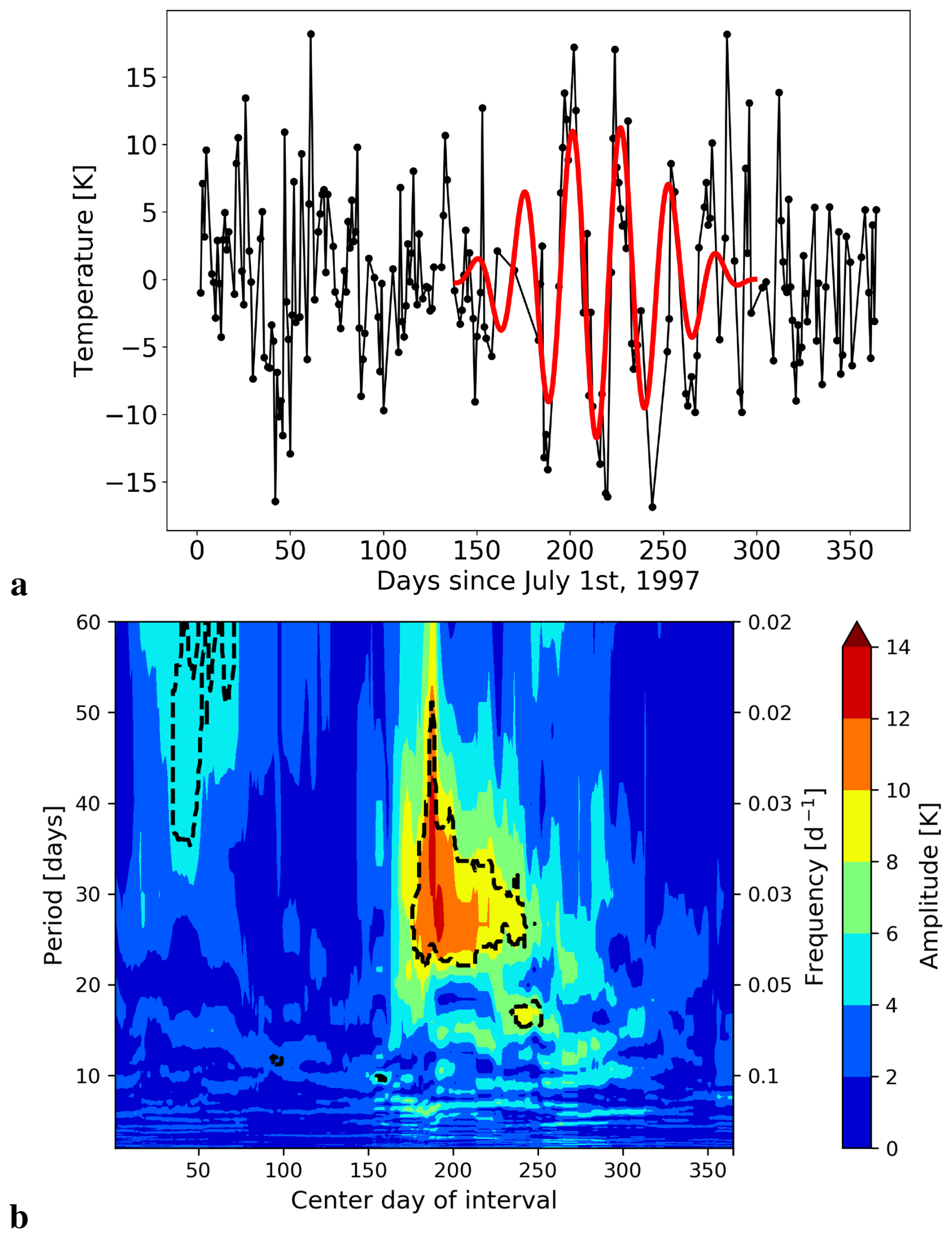
Figure 7 Example for an event with a large temperature fluctuation with a period of around 28 d. (a) The temperature time series after subtracting the seasonal variations is shown as black curve (the seasonal fit was centred in winter). The red curve is the fit to the data in the middle part of the time series. The x axis show days since 1 July 1997. (b) LSP result for the amplitudes of periodic fluctuations over the winter 1997/1998. The x axis show the centre days of the windows since 1 July 1997 and the y axis show the period and frequency of the fluctuations, respectively. The amplitude is displayed colour coded. The LSP was calculated with a fixed window of 60 d to focus on the long periods and slightly smooth the results for better visibility. Furthermore, the influence of the partly larger data gaps is reduced.

Another period range that is frequently observed for planetary waves in the MLT region lies in the region around 16 d (e.g. Espy et al., 1997; Luo et al., 2000; French et al., 2005; Jarvis, 2006; Day and Mitchell, 2010b; French and Kelkociuk, 2011; Takahashi et al., 2013). We also observe a smaller peak in the histogram in the period range around 15 d (see Fig. 3) and we would assign this as a quasi-16-day wave, too. Note here that the resolution of the LSP (FWHM) which is about $\mathrm{1}/T$ (see Cumming et al., 1999), where T is the length of the time window (in this period range 25 d). This means that single observations with periods of 15 or 16 d are not significantly different. Another wave that has frequently been mentioned in literature is the quasi-5-day wave (e.g. Wu et al., 1994; Jarvis, 2006; Day and Mitchell, 2010a). In our observations we observe also a larger number of significant events in this period range. More precisely, we observe two peaks, one at about 5 d and one at about 6 d However, due to the resolution of the LSP, these two peaks would not be significantly different for single detections. Thus, we would assign all of these observations to the quasi-5-day wave. The quasi-10-day wave is also a known wave type in the atmosphere (e.g. Jarvis, 2006; Takahashi et al., 2013; Forbes and Zhang, 2015). In our observations we see a very prominent peak at about 10 d and two additional peaks nearby at slightly above 8 d and slightly below 12 d. According to the resolution of the LSP results we would assign all observations in this range to the quasi-10-day wave. The quasi-2-day wave is also a prominent feature in the MLT region (e.g. Wu et al., 1993; Takahashi et al., 2005; López-González et al., 2009; Hecht et al., 2010; Yue et al., 2012; Reisin, 2021). We observed an enhanced occurrence frequency in this period range (see Fig. 3), too. Relative to its period length the quasi-2-day wave is a prominent feature of our observations. We also observed many events in the period range above 30 d. Planetary waves with very similar periods have also been reported for other observation sites in Antarctica (Espy et al., 2005; Stockwell et al., 2007; French and Kelkociuk, 2011).

Observations of different Rossby wave modes could possibly explain a number of our observations, e.g. the Rossby wave mode (1,3) 16-day-wave (Kasahara, 1980; Salby, 1981b; Espy et al., 1997) or the Rossby wave mode (3,0) the quasi-2-day wave (Kasahara, 1980; Wu et al., 1993; López-González et al., 2009; Yue et al., 2012), and cause the observations to appear primarily in certain period ranges. However, a better constraint of the origin of the waves and their complete structure would need additional data and further investigations which is beyond the scope of this paper.

The seasonal variation of the occurrence frequency of the waves varies for different types of waves. In the period range below 20 d we observe two maxima around the spring equinox in April and in late summer (August/September), whereby the major part of the observations around the equinoxes and in summer stem from waves with periods below 10 d (compare Fig. 4). In the case of waves with longer periods (>20 d) a large maximum in winter and late fall is observed. Observations in summer and other seasons are comparable small (compare Fig. 4).

A larger occurrence frequency for waves with shorter periods in other seasons than winter has also been observed by others. Reisin (2021) analysed the seasonality of the quasi-2-day wave and observed a larger number of events in Southern hemisphere summer than winter. The analysis by López-González et al. (2009) revealed higher occurrence probabilities for the quasi-2-day wave observed in OH temperatures in the period from about January to August. in the same study the probability for the quasi-5-day wave shows local maxima in March/April, August/September and November. Wu et al. (1994) analysed two years of HDRI (High Resolution Doppler Imager) data and observed wave events of the quasi-5-day wave mainly in April/May and in September to October. Radar observations over India showed larger activities of the 6.5 d wave around the equinoxes (April/May and September/October) (Kishore et al., 2004). Riggin et al. (2006) also observed larger events in April/May when analysing SABER data over a time period of three years. Observations in both hemispheres at polar sites showed strong wave activity for the 5 d wave in winter and late summer (August/September) but no significant events at equinoxes (Day and Mitchell, 2010a). In a former study of the GRIPS observations at Wuppertal the authors also reported a larger amount of events in summer time in the case of planetary waves with shorter periods (Bittner et al., 2000). In total, the seasonal variation of the wave activity in the case of shorter periods observed at Wuppertal agrees quite well with other observations. The observation of large planetary wave events in summer cannot be explained with the excitation of these waves in the troposphere and their propagation up to the MLT region, because the mean stratospheric flow in summer prevents these upward propagation of most waves (e.g. Charney and Drazin, 1961). Thus, other mechanisms are necessary to explain the observations. Two main mechanism are discussed in previous work. On the one hand, the waves can be exited at higher altitudes and propagate upwards afterwards and, on the other hand, ducting from the winter hemisphere to the summer hemisphere could take place (e.g. Bittner et al., 2000; Riggin et al., 2006; Day and Mitchell, 2010a, and references therein). In the period range between 10 and 20 d we observe wave events in most of the seasons except for summer. The quasi-16-day wave and a part of the observations of the quasi-10-day wave are mainly responsible for this. Most of the other studies found in literature also report on similar seasonal distributions. For the quasi-10-day wave Forbes and Zhang (2015) presented maximum activity in winter and around the equinoxes in mid-latitudes. The analysis of OH temperatures by López-González et al. (2009) showed the by far largest occurrence probability of the quasi-10-day in September and October and some smaller probability in the time period from February to June. No observations in July and August are reported in the study. In the case of the quasi-16-day wave the picture is quite similar with stronger activity in winter and only minor activity in summer months (Luo et al., 2000; Day and Mitchell, 2010b). Nonetheless, the quasi-16-day wave has also been observed in summer (e.g. Espy et al., 1997). Discussed mechanism are again local phenomena and ducting from the winter to the summer hemisphere (see Espy et al., 1997; Luo et al., 2000, and references therin).

In the case of wave events with periods longer than 20 d we observe a large summer to winter differences. A huge number of events took place in winter time or late fall and only a very small number of events in summer. As already mentioned this is expected because of the wave filtering in summer that prevents the wave propagation to the MLT region. These findings are also confirmed by previous other studies. The observation of the 28 d wave event reported by Zhao et al. (2019) also took place in winter. Similarly, Stockwell et al. (2007) report that the largest activity of waves in the period range from 30 to 50 d is observed in late winter.

4.2 Long-term behaviour of wave activity

We see a main long-periodic fluctuation with a period of about 20 years in the long-term behaviour of the wave activity. This can be seen in two of the three different proxies. Of the two new proxies only the yearly mean amplitude of the significant events shows a clear long-term behaviour. Therefore, the standard deviation, which is mainly determined by the amplitude of the significant fluctuations in most years, also shows a very similar long-term behaviour. The fact, that the time series of the weighted sum of days with significant results does not show the same long-period fluctuation suggests that in years with higher activity during the quasi-bidecadal oscillation (for example mid-1990s) not more events are expected but events with larger amplitudes than in the years with lower activity (for example around 2005).

The quasi-bidecadal oscillation of the standard deviation has also been observed by Höppner and Bittner (2007) for a shorter time interval of observations (until 2005). Thus, their findings agree well with ours and the wave activity observed by the standard deviation proxy continues in this quasi-bidecadal oscillatory way. Jarvis (2006) also observed a quasi-bidecadal oscillation in the wave activity of the 5 d planetary wave. Like us Jarvis (2006) observed the quasi-bidecadal oscillation in the residual planetary wave amplitudes. The observed change lies in the range of about 10 % which is in line with our observations here, where we see a change of roughly ±1 K and a mean amplitude of about 8 K. In contrast to our findings, where we see the quasi-bidecadal oscillation in the mean over all periods in the range from 2 to 60 d, Jarvis (2006) observed the long-term fluctuation for the 5 d planetary wave only and not for the 10 and 16 d planetary wave.

In former studies of the OH^*3,1) rotational temperatures we already observed the quasi-bidecadal oscillation in yearly mean temperature observations (Kalicinsky et al., 2016, 2018, 2024). The phase of the quasi-bidecadal oscillation of the temperature observations is nearly the same as that of the mean amplitude and the standard deviation of the residuals, respectively. All of the time series show maxima around the mid-1990s and around 2015/2016 in addition to a minimum around 2005. This means the larger amplitudes of the significant wave events occur together with enhanced yearly mean temperatures and vice versa. We also observed the quasi-bidecadal oscillation in other altitudes such as the mesosphere and stratosphere with alternating sign from one atmospheric layer to the other (stratosphere and lower thermosphere (GRIPS OH^*(3,1) rotational temperatures) are in phase and the mesosphere is shifted by 180°) (Kalicinsky et al., 2018) and also on ground (Kalicinsky and Koppmann, 2022). This temperature oscillation in the atmosphere might influence other atmospheric parameters such as the wind and, therefore, also influence the wave filtering. Likely, only in certain years the conditions are favourable for waves with smaller amplitudes to reach higher altitudes, whereas in other years only waves with amplitudes that are large enough reach the observation altitude of the GRIPS instrument. But a complete analysis of this hypothesis will require additional data and is beyond the scope of this paper.

Additionally, we found some indications for a quasi-quadrennial oscillation of the weighted sum of days of significant events, which is a proxy for wave activity that also largely takes into account the length of the events. French et al. (2020) observed a very similar quasi-quadrennial oscillation for the OH^* rotational temperatures above Davis, Antarctica. The phase of the two oscillations is also quite similar with the Wuppertal oscillation slightly preceding by up to one year. French et al. (2020) discussed a potential role of planetary or tidal waves in their quasi-quadrennial oscillation. This would agree well with our observations and could possibly explain the time lag. Nonetheless, a complete analysis would require additional data and is beyond the scope of this paper. Furthermore, a longer time series and a potentially increased significance of the results would be beneficial as well.

5 Summary and conclusions

We analysed more than 30 years of OH(3,1) rotational temperatures observed from Wuppertal with respect to periodic fluctuations in the period range from 2 to 60 d. Fluctuations with a period around 28 d are the main fluctuation observed in this era. Other period ranges which are often detected in the observations are around 2 d, 5 to 6 d, 8 to 12 d, and around 15 d.

Most of the waves are observed in winter time because of the different wave filtering in summer and winter, i.e. the conditions in winter are typically more favourable for waves to reach higher altitudes. This winter to summer difference is not universal for all waves. It holds for waves with longer periods, but it breaks off in the case of shorter periods below about 20 d. These waves with shorter periods occur more evenly distributed across the year with even a larger number of events around the equinoxes. Thereby waves with periods below 10 d are nearly completely responsible for the observations in summer and to a large degree for that around equinoxes.

The mean amplitude of all observed significant events is about 8 K, whereby the amplitudes range from about 2 to 16 K. A significant difference for the distribution of the amplitudes dependent on the period range was not observed.

The analysis of the long-term behaviour of the wave activity revealed a quasi-bidecadal oscillation. This oscillation is observed in two wave proxies, the standard deviation of the temperature residuals and the mean amplitude of the significant events within a year. Since the last wave proxy, the amplitude weighted sum of days with significant results, does not show this fluctuation, the conclusion is that the amplitude is the quantity that shows the quasi-bidecadal oscillation. This means, that in certain years not more events but events with larger amplitudes are expected, whereas in other years the mean amplitude of the events is smaller. The quasi-bidecadal oscillation is in phase with the oscillation of the yearly mean temperatures themselves. A connection between changes in the background temperature field and, thus, also other parameters, may influence the wave filtering and lead to the observation of the quasi-bidecadal fluctuation of the wave activity.