Impact of small-scale orography on deep boundary layer evolution and structure over the Tibetan Plateau

We investigate how small-scale orography influences the evolution and structure of the exceptionally deep convective boundary layer (CBL) over the Tibetan Plateau (TiP). Using large-eddy simulations (LES) at 50 m resolution under semi-idealized dry conditions, we compare four experiments over an elevated plateau (4.2 km above mean sea level (a.m.s.l.)): FLAT (no local orography), REAL (realistic terrain), and FLATu10/REALu10 (including a 10 m s⁻¹ upper-level wind). ABL height is diagnosed using a passive tracer method and cross-validated against turbulence and thermodynamic fields. All simulations produce a very deep CBL, reaching ∼9 km a.m.s.l. by late afternoon, consistent with the record-high values observed over the TiP.

Small-scale orography accelerates early CBL growth and anchors persistent thermals. REAL shows only a modest (∼1 %–2 %) increase in domain-mean ABL height relative to FLAT, yet locally the ABL is up to 20 % higher over the ridge, revealing strong spatial heterogeneity. Imposed upper-level shear (FLATu10, REALu10) produces deeper and more laterally uniform CBLs, with shear-driven rolls increasing the mean ABL height by roughly 10 %–15 % and homogenizing the tracer field. Orography primarily affects the upper tail of the distribution, with ridge-top 99th-percentile ABL heights exceeding flat-terrain values by 10 %–20 %, while shear is the dominant control on domain-mean deepening.

These results show that unresolved fine-scale orography and shear strongly modulate both the depth and spatial variability of the TiP CBL, and can substantially influence entrainment under weak stability. Their omission may lead weather and climate models to underestimate CBL growth and vertical exchange over high-altitude regions.

1 Introduction

The atmospheric boundary layer (ABL) over the Tibetan Plateau (TiP) plays a crucial role in the climate system, regional weather, and air quality. Despite its importance, many aspects of the TiP's boundary layer remain poorly understood due to sparse observations over this remote high-altitude region (Che and Zhao, 2021). One distinguishing feature of the TiP's ABL is its extraordinary depth (Chen and Ma, 2025). Summertime convective boundary layers (CBLs) commonly achieve 2–4 km heights above ground level (a.g.l.) across the plateau, far deeper than over lowland terrain. Even higher extremes have been observed under favorable conditions. In winter and spring, for example, ABL heights of 9 km above mean sea level (m.s.l.) have been recorded (Chen et al., 2013), effectively bringing the boundary layer into contact with the tropopause and enabling exchange of air between the surface and lower stratosphere (Chen et al., 2011). Such deep vertical mixing has important implications for atmospheric composition: the TiP is a global hotspot for stratospheric intrusions, which can elevate surface ozone and other tracer gases over the plateau (Yin et al., 2023; Ojha et al., 2017). These characteristics make the TiP ABL a unique and influential component of the Asian climate system.

Observational and modeling studies have begun to uncover the controls on the plateau's deep ABL and vigorous vertical mixing. The intense sensible heat flux from the heated surface creates strong convective turbulence, allowing the ABL to grow to great heights (Zhao et al., 2023). In dry and cloud-free regions, this effect is especially pronounced, as more incoming solar radiation is converted into turbulent heat flux (Zhang et al., 2011). Accordingly, the western and central TiP – characterized by low soil moisture, sparse cloud cover, and large sensible heat fluxes – tend to develop deeper daytime ABLs than the wetter eastern plateau (Che and Zhao, 2021; Santanello et al., 2005). Moisture availability also modulates boundary layer growth in complex ways: when the surface is too dry, limited moisture constrains convection; when it's too wet, early cloud formation can reduce solar heating and inhibit further growth (Xu et al., 2021). High-resolution simulations have shown that there is often an optimal intermediate soil moisture that produces the most vigorous convective development in the TiP's landscape (Gerken et al., 2015). In addition to aforementioned factors, atmospheric stratification aloft also plays a crucial role: a weakly stable free atmosphere permits thermals to rise higher before stopping. Indeed, the extremely deep springtime ABLs observed over the plateau have been attributed to weak stability in the lower troposphere (Chen et al., 2016), rather than surface conditions alone. In summary, the ABL depth over the TiP is governed by a combination of intense surface heating, moisture availability, cloud feedbacks, and the thermal structure of the atmosphere above.

Accurately representing meteorology and ABL processes in mountainous terrain remains a major challenge for numerical weather and climate models. The ABL over complex orography is influenced by processes across multiple scales, from thermally driven slope and valley winds to mountain-wave breaking, heterogeneous turbulence, and land–atmosphere interactions (Lehner and Rotach, 2018; Serafin et al., 2018). Field studies further illustrate how local orography interacts with regional flow: along the eastern margin of the plateau, the interaction of plateau orography with regional circulations produces a regular alternation of low-level wind directions that governs weather in the adjacent Sichuan Basin (Li and Gao, 2007). Similarly, a Himalayan valley study showed that the alignment of synoptic winds with valley geometry dramatically affected ABL growth, with strong along-valley westerlies promoting deep (9 km a.m.s.l.) mixing layers, while weaker cross-valley winds led to a much shallower ABL despite comparable surface heating (Lai et al., 2021). These examples demonstrate that orography can exert a first-order control on ABL depth and structure.

Yet the specific contribution of smaller-scale terrain features to the plateau's deep convective boundary layer remains poorly quantified. Most modeling studies have emphasized regional-scale influences while treating the terrain in smoothed or idealized form. However, even modest heterogeneities such as land–lake thermal contrasts can drive secondary circulations that alter turbulence and vertical transport (Zhang et al., 2021). Despite advances toward convection-permitting and cloud-resolving resolutions, models continue to face difficulties in capturing boundary-layer dynamics across scales (Solanki et al., 2019; Rajput et al., 2022; Singh et al., 2016; Guo et al., 2021). For example, Wagner et al. (2014) demonstrated in an idealized valley that unresolved terrain, rather than turbulence alone, can strongly alter ABL structure as resolution coarsens. Likewise, even LES at 𝒪(100–300 m) resolution can suffer scale-transition issues, with excessive or insufficient turbulent mixing depending on the scheme used (Poll et al., 2022; Goger et al., 2022; Singh et al., 2021). Intercomparison studies further confirm that no single ABL parameterization performs optimally across all conditions, underscoring the need for systematic validation and development (Singh et al., 2024). Even modern high-resolution reanalyses face similar challenges: ERA5 (with ∼30 km grid spacing) captures the general diurnal cycle of the plateau's boundary layer but often underestimates the deepest observed ABL peaks (Slättberg et al., 2022). The scarcity of in situ observations in the plateau's remote interior, especially over the western TiP, further complicates efforts to determine how small-scale terrain modulates ABL growth and mixing (Che and Zhao, 2021). Consequently, the role of the myriad hills, ridges, and gentle slopes that characterize the plateau's surface in shaping vertical exchange remains an open question.

These challenges motivate the present work, which examines the role of small-scale, unresolved orography on ABL height using high-resolution simulations. Our study explicitly focuses on how sub-kilometer orography influences ABL evolution, a key aspect that remains underexplored but is critical for improving predictions in complex terrain. We design a set of semi-idealized LES that isolate the influence of small-scale terrain and shear on deep CBL growth over an elevated plateau. The experiments compare a flat-plateau baseline with three other configurations that include a realistic orography, and upper-level winds. Passive tracers are used to diagnose vertical mixing and entrainment. With these simulations, we quantify both domain-averaged and localized orographic effects under weak stability aloft.

Details of the model configuration, terrain processing, and experiment design are provided in Sect. 2. Section 3 compiles the diagnostics of the LES, along with turbulence analysis and statistics of the diagnosed ABL heights. In Sect. 4, we summarize our findings and implications of the study, as well as providing its context.

2 Methods

2.1 Numerical Model

The Cloud Model 1 (CM1) (Bryan and Fritsch, 2002) version 21.1 is utilized in LES mode. CM1 is an idealized, fully compressible, non-hydrostatic, cloud-resolving numerical atmospheric model. The simulation starts at 09:00 local time (LT) (LT corresponds to the Beijing standard time, UTC+8), shortly after local sunrise, and runs until 20:00 LT (11 h). The first two hours of the simulation are considered spin-up for the model to achieve a reasonable atmospheric state, and are discarded from the analysis. The simulations are conducted under dry conditions without any microphysics scheme, and latent heat fluxes are excluded. Subgrid-scale turbulence is parameterized by the 1.5-order TKE closure from Deardorff (1980).

Advection and momentum transport are handled by the Weighted Essentially Non-Oscillatory (WENO) scheme (Jiang and Shu, 1996), with improved smoothness indicators included (Borges et al., 2008). The scheme guarantees positive-definiteness and scalar mass conservation of passive tracers. For time integration, the Klemp–Wilhelmson time-splitting method (Klemp and Wilhelmson, 1978) is used, which keeps acoustic and gravity waves separated from the meteorologically relevant modes, thereby increasing computational efficiency.

The model domain is defined with a 50 m horizontal grid spacing and a size of $\mathrm{25}\mathrm{km}\times \mathrm{25}\mathrm{km}\times \mathrm{14}\mathrm{km}$, consisting of $\mathrm{500}\times \mathrm{500}\times \mathrm{216}$ grid points. The vertical grid spacing is set to 20 m below 300 m altitude, then increases linearly from 20 to 100 m at 10 km, and then maintains constant spacing until 14 km. Previous studies have demonstrated that the CM1 model performs well for both idealized and semi-idealized setups when studying mountain-induced turbulence (Mulholland et al., 2021; Weinkaemmerer et al., 2022). The model applies a semi-slip condition at the lower boundary and a free-slip condition for winds at the top boundary, where the semi-slip condition allows tangential wind to respond to surface drag while still permitting some slip (i.e. the near-surface wind is reduced but not forced to zero). The lateral boundary conditions are periodic representative of extensive mountainous terrain.

To simulate the high ABL of 9515 m m.s.l. reported on 4 March 2008 (Chen et al., 2016), the model uses an idealized sounding as the initial condition: a 300 m surface mixed layer with constant potential temperature θ=306.8 K, followed by a stable layer with a weak lapse rate of 0.1 K (100 m)⁻¹ until the top of the domain. The weak stability above the initial mixed layer was chosen to represent specific pre-monsoon conditions over the TiP, where a more southerly jet position is associated with enhanced upper-level potential vorticity and a nearly dry-adiabatic free troposphere (Chen et al., 2016). The relative humidity profile is constant at 0 %, as well as the background wind speed profile ($u=\mathrm{1}\mathrm{m}{\mathrm{s}}^{-\mathrm{1}}$). These initial conditions ensure favorable conditions for deep CBL growth. A Rayleigh damping layer is introduced above 11.2 km altitude to the top of the model domain, with a damping time of 300 s. The Coriolis parameter is set to zero.

The surface exchange coefficients are constant, based on Monin–Obukhov similarity theory using a prescribed surface roughness length of 0.01 m. The diurnal cycle of surface sensible heat flux is prescribed as follows: starting at zero at 09:00 LT, it follows a sine function peaking at 180 W m⁻² after six hours (15:00 LT) and returning to zero after 11 h (20:00 LT). These prescribed flux values are adopted based on the observed surface fluxes obtained from the authors of Chen et al. (2016).

To study mixing sources and to help in boundary layer height diagnosis, two passive tracers are introduced into the model. One is a surface-based tracer emitted with a constant surface flux $J_{\text{surf.}}=\mathrm{4}\times {\mathrm{10}}^{-\mathrm{5}}\mathrm{kg}{\mathrm{m}}^{-\mathrm{2}}{\mathrm{s}}^{-\mathrm{1}}$ with no initial concentration ($c_{\mathrm{0},\text{surf.}}=\mathrm{0}$). The other is an upper-level tracer, initialized with a mixing ratio of $c_{\mathrm{0},\text{up.}}=\mathrm{1000}$ ppm above 4 km height above plain level (APL) and has no flux (J_up.=0).

2.2 Experiments and Data

The study focuses on the western Tibetan Plateau near the Gerze station (32.17° N, 84.03° E; Fig. 1a). The selected region (Fig. 1b) is intended to represent the influence of heterogeneous terrain, with mountains rising by approximately 1400 m, on boundary-layer evolution. For early March reference period, local sunrise at this location occurs at approximately 08:47 LT. Terrain data were obtained from the Shuttle Radar Topography Mission (SRTM) at a resolution of ∼30 m (U. S. Geological Survey, 2015), cropped to the model domain, reprojected to UTM Zone 45N, and interpolated to the CM1 Cartesian grid. To ensure smooth lateral transitions, the outer 4 km of the domain (outside the ellipse in Fig. 1b) were tapered to the minimum elevation of 4200 m m.s.l. (≡0 m APL) using a super-Gaussian mask (see Appendix B). A single Gaussian filter with σ=75 m was then applied (Fig. 1c) to reduce small-scale roughness while retaining the dominant terrain features. The resulting smoothed surface (Fig. 1d) serves as the basis for the simulations, including the two subdomains R-FLAT and R-TOPO used later in the statistical analysis.

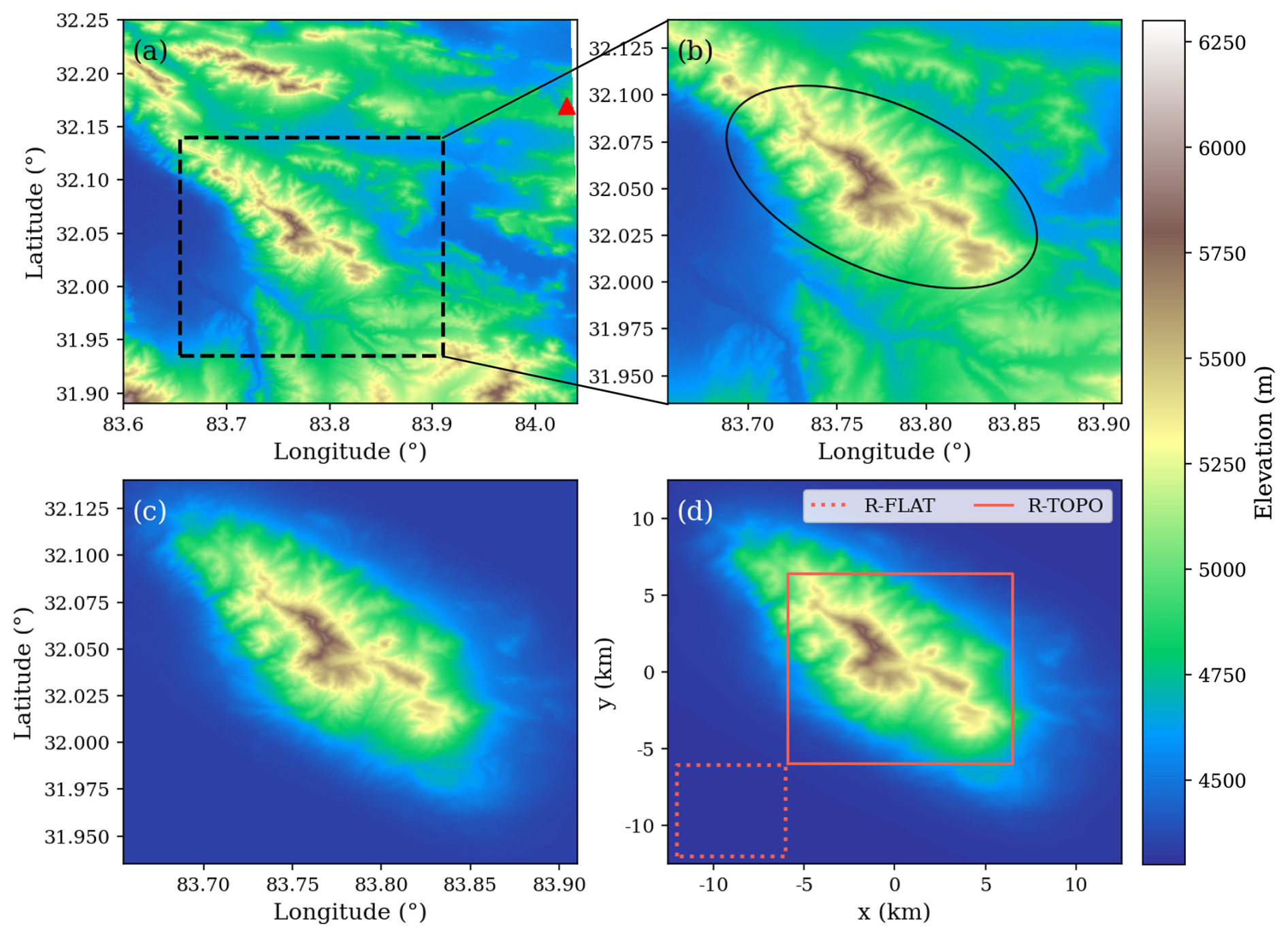
Figure 1 Shaded-relief terrain elevations used in the study. (a) Broader region of the western Tibetan Plateau, with the Gerze station shown as a red triangle. (b) Zoomed view of the complex ridge–valley system. (c) Same zoomed region after applying the super-Gaussian tapering outside the ellipse to smooth the lateral boundaries. (d) Final terrain field used in the REAL simulation, obtained by applying a 2D Gaussian filter to panel (c). The locations of the R-TOPO and R-FLAT subdomains used for the statistical analysis are indicated by orange rectangles. Elevation data are based on SRTM and reprojected to a Cartesian grid.

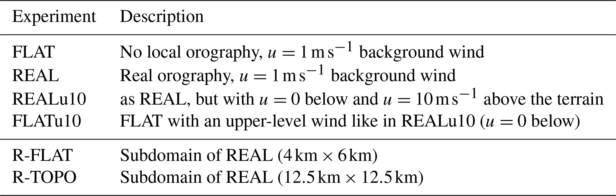
The small-scale orography contains slopes up to about 36° and characteristic ridge–valley structures typical of the central Tibetan Plateau (Fig. 1a), with elevation differences up to ∼1.4 km and ridge widths of 5–10 km. Four experiments are conducted: REAL, which uses the realistic orography; FLAT, which represents an elevated plateau at 4200 MSL without local orography; and the corresponding experiments REALu10 and FLATu10, which include an imposed large-scale background wind. In REALu10 and FLATu10, the horizontal wind speed increases linearly above the mountain crest, reaching $u=\mathrm{10}\mathrm{m}{\mathrm{s}}^{-\mathrm{1}}$, in order to introduce a non-zero plateau-scale flow comparable to that reported by Chen et al. (2016, their Fig. 5), while keeping near-surface winds weak to avoid triggering strong orographic waves during initialization. The base elevation in FLAT and along the smoothed edges of REAL and REALu10 corresponds to the minimum elevation within the realistic terrain (Fig. 1a). The full list of experiments and their descriptions is provided in Table 1.

Table 1 List of the experiments and the subdomains. R-TOPO and R-FLAT refer to the subdomains depicted in Fig. 1c.

2.3 Analysis methods

2.3.1 Reynolds averaging and flow decomposition

One of the main advantages of the LES approach is its ability to explicitly resolve the large, energy-containing turbulent structures. As a result, the model output fields are inherently turbulent. It is therefore customary to decompose a turbulent flow variable a(x,t) into a mean and a fluctuating component:

$$\begin{array}{}\text{(1)}& a(\mathit{x},t)=\stackrel{\mathrm{‾}}{a}(\mathit{x},t)+a^{\prime }(\mathit{x},t),\end{array}$$

where $\stackrel{\mathrm{‾}}{a}$ denotes a mean component and a^′ the turbulent fluctuation.

In the present study, the mean field does not represent a classical ensemble or Reynolds average in the strict statistical sense. Instead, it is a hybrid space–time decomposition designed to separate turbulent-scale motions from larger-scale, sub-mesoscale variability in a spatially heterogeneous domain. Specifically, the mean field is constructed by applying a two-dimensional Gaussian spatial filter to the time-averaged variable ${\stackrel{\mathrm{̃}}{a}}^t$:

$$\begin{array}{}\text{(2)}& \stackrel{\mathrm{‾}}{a}(x,y,z,t)\equiv \underset{A}{\int }{\stackrel{\mathrm{̃}}{a}}^t(x^{\prime },y^{\prime },z,t)G(x-x^{\prime },y-y^{\prime }),\end{array}$$

where G(x,y) is a two-dimensional Gaussian kernel and A denotes the horizontal domain.

This approach is motivated by the limitations of purely temporal or purely spatial averaging in complex terrain. Time averaging alone yields insufficient sampling for robust turbulent statistics, while domain-wide spatial averaging is inappropriate due to strong orographic heterogeneity. The combined space–time filtering therefore serves as a practical approximation to an ensemble mean, isolating the dominant turbulent motions while retaining spatial structure tied to the terrain.

The domain-averaged variable at the interpolated vertical levels is defined as:

$$\begin{array}{}\text{(3)}& \widehat{a}(z,t)={\displaystyle \frac{\mathrm{1}}{A}}\underset{A}{\int }\stackrel{\mathrm{‾}}{a}(x,y,z,t)\mathrm{d}x\mathrm{d}y,\end{array}$$

and is used to construct vertical profiles of mean quantities.

In practice, the procedure was implemented by first performing online time-averaging of the instantaneous fields at 30 s intervals over 30 min windows (cf. Weinkaemmerer et al., 2022), yielding ${\stackrel{\mathrm{̃}}{a}}^t$. A two-dimensional Gaussian filter with a standard deviation of σ=500 m and a cutoff radius of 4σ (corresponding to a total support width of 4 km) was then applied using the gaussian_filter function from scipy.ndimage.

The chosen filter scale was selected to match the dominant horizontal length scales of the largest turbulent structures resolved by the LES, including convective thermals and shear-organized roll vortices, which typically span O(1 km) in diameter. Sensitivity tests using smaller (σ=250 m) and larger (σ=1 km) smoothing lengths yielded consistent qualitative results, indicating that the decomposition is not sensitive to the exact choice of filter width. Compared to pure time averaging, this combined space–time filtering more effectively isolates turbulence-scale variability in a strongly heterogeneous environment.

Using the definition given in Eq. (2), the variance can be written as

$$\begin{array}{}\text{(4)}& \stackrel{\mathrm{‾}}{{a^{\prime }}^{\mathrm{2}}}=\stackrel{\mathrm{‾}}{a^{\mathrm{2}}}-{\stackrel{\mathrm{‾}}{a}}^{\mathrm{2}}\end{array}$$

where $\stackrel{\mathrm{‾}}{a^{\mathrm{2}}}$ is calculated by the above procedure: (1) online time-averaging of a², and (2) applying Gaussian filter to a². The above flow decomposition and notation are used consistently throughout the manuscript.

2.3.2 Diagnostic Boundary Layer Height via Tracer Method

Boundary-layer height is diagnosed using both a passive-tracer method and a conventional parcel-based estimate (Duncan et al., 2022) (see Appendix A for details and a quantitative comparison). The parcel method follows a surface parcel that is lifted dry adiabatically and identifies the BL top where the parcel becomes neutrally or slightly negatively buoyant relative to the environment (a standard approach in CBL studies). While thermodynamically meaningful, this method can be sensitive to local inversions and fine vertical layering, especially in very deep and weakly stratified boundary layers.

To obtain a measure that is more directly tied to turbulent mixing and tracer transport, we primarily use a tracer-based diagnostic. For each model column c and model level z_k, let ${\stackrel{\mathrm{‾}}{\mathit{\varphi }}}_c\left(z_k\right)$ denote the ensemble-mean tracer concentration. We define a two-level moving average

$${\stackrel{\mathrm{‾}}{\mathit{\varphi }}}_c^{\text{mov}}\left(z_k\right)={\displaystyle \frac{\mathrm{1}}{\mathrm{2}}}\left[{\stackrel{\mathrm{‾}}{\mathit{\varphi }}}_c\right(z_k)+{\stackrel{\mathrm{‾}}{\mathit{\varphi }}}_c(z_{k+\mathrm{1}}\left)\right],$$

and a cumulative column-mean above the surface,

$${\stackrel{\mathrm{‾}}{\mathit{\varphi }}}_c^{\text{cum}}\left(z_k\right)={\displaystyle \frac{\mathrm{1}}{N_k}}\sum _{j=k_{\mathrm{6}}}^k{\stackrel{\mathrm{‾}}{\mathit{\varphi }}}_c\left(z_j\right),$$

where k₆ is the index of the sixth level used in the average (we exclude the lowest five model levels to avoid the strong near-surface peak), and $N_k=k-k_{\mathrm{6}}+\mathrm{1}$ is the number of levels in the sum. The ABL depth in column c is then diagnosed as the height z_i,c of the first level z_k that satisfies

$${\stackrel{\mathrm{‾}}{\mathit{\varphi }}}_c^{\text{mov}}\left(z_k\right)\le \mathrm{0.05}{\stackrel{\mathrm{‾}}{\mathit{\varphi }}}_c^{\text{cum}}\left(z_k\right).$$

Once this criterion is met, we identify z_i,c as the mixed-layer top in that column, and the levels below z_i,c as the well-mixed layer.

This tracer-based diagnostic provides a dynamically adaptive and spatially consistent estimate of BL height that is closely linked to the actual extent of turbulent mixing, and it remains robust in complex terrain and very deep, weakly stratified layers. As shown in Appendix A, it agrees well with the parcel-based estimate on average, but yields smoother and more coherent spatial fields, which is why we adopt it as our primary BL-height metric.

3 Results

3.1 Mesoscale flow evolution

Figure 2 shows the evolution of domain-averaged potential temperature ($\widehat{\mathit{\theta }}$) and $\widehat{u}$-wind profiles. The $\widehat{\mathit{\theta }}$ profile shows the atmosphere heating from the surface, with a sustained unstable surface layer, followed by a deep and growing adiabatic, but statically unstable layer. The ABL height extends up to more than 9 km a.m.s.l. at 19:00 LT for all experiments, but slightly higher in REALu10. The FLAT wind profiles remain close to the imposed background wind, except within the lowest 0.5 km where surface drag reduces the flow. In contrast, the REAL experiments exhibit more nuanced wind structures due to the combined effects of surface drag, complex orography, thermal winds, plain-to-mountain circulations, and upper-level recirculation. Nevertheless, their late-day structure becomes broadly similar. The REALu10 and FLATu10 profiles are highly comparable: they begin with strong vertical shear, but downward momentum transport gradually produces a finite mean wind throughout the boundary layer and a shear layer across the entrainment zone.

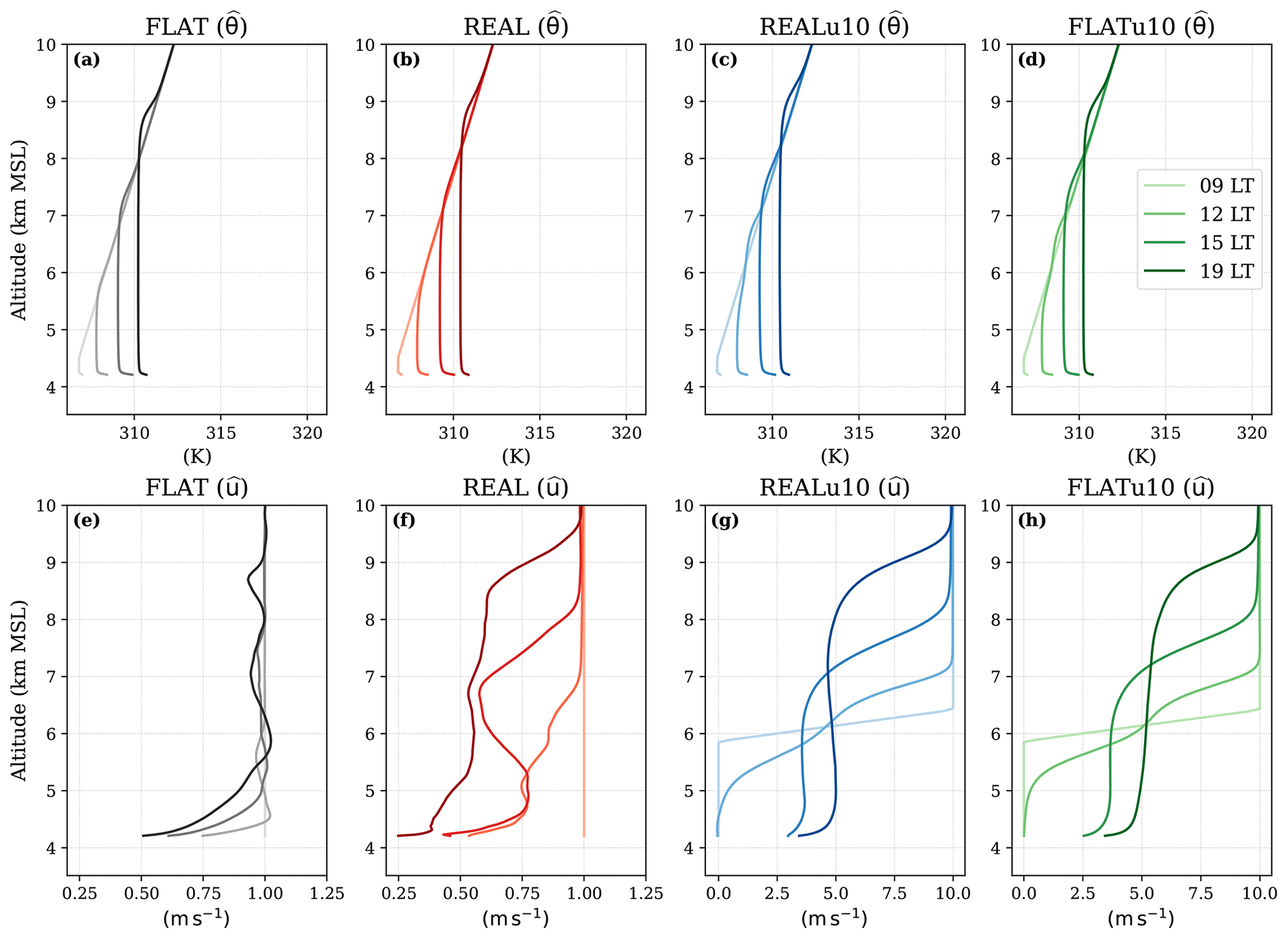
Figure 2 Diurnal evolution of the domain-averaged (Eq. 3) potential temperature (top row) and u-wind component (bottom row), interpolated to horizontal surfaces. Colors indicate time, with darker shades corresponding to later times; the legend indicates specific times and the color scale used in FLATu10.

However, the domain-averaged profiles alone do not clearly capture structural differences in the CBL. To address this, Fig. 3 depicts the spatial structure of convective flow at 15:00 LT, when the CBL is fully developed, showing the ensemble mean vertical velocity ($\stackrel{\mathrm{‾}}{u}$) and potential temperature ($\stackrel{\mathrm{‾}}{\mathit{\theta }}$) fields, which reveal distinct patterns among the experiments. The spatial distribution of the thermally-driven flow differs slightly between the FLAT and REAL terrain configurations due to underlying surface heterogeneity. In FLAT (Fig. 3a and e), the quasi-stationary horizontal structures of updrafts (positive $\stackrel{\mathrm{‾}}{w}$) and downdrafts (negative $\stackrel{\mathrm{‾}}{w}$) are visible, reflecting the homogeneity of the surface. Convective thermals develop through turbulent interactions in the absence of fixed surface features, leading to temporally and spatially variable convective structures. In contrast, the thermal flow in REAL (Fig. 3b and f) is slightly more organized. The updrafts are aligned with orographic features, indicating a mesoscale flow signal. Elevated terrain serves as a main factor in the response to surface heating, and generates persistent, thermally-driven updrafts. This results in a more structured and spatially confined flow organization, with enhanced activity concentrated over and adjacent to mountainous regions.

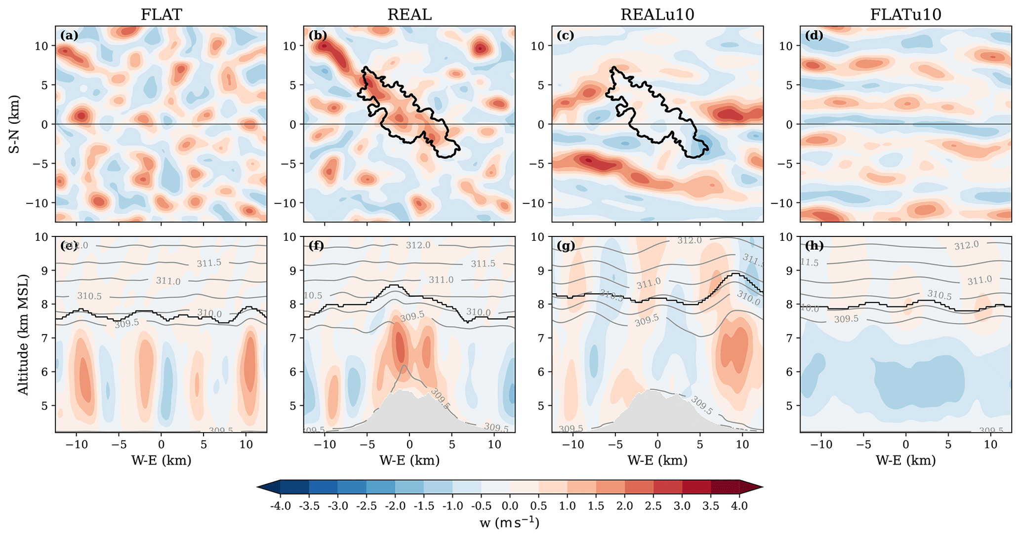
Figure 3 Snapshot of mean vertical velocity $\stackrel{\mathrm{‾}}{w}$ for the different experiments at 15:00 LT. Top: horizontal cross-sections at 6 km a.m.s.l., with the 800 m APL orography isoline indicated by a black contour. Bottom: vertical cross-sections of $\stackrel{\mathrm{‾}}{w}$ at y=0 with $\stackrel{\mathrm{‾}}{\mathit{\theta }}$ (gray contours) and the diagnosed boundary-layer height (black contour; see Sect. 2.3.2).

In stark contrast is FLATu10 (Fig. 3d and h), where convection results in elongated streaks in the direction of the mean wind. These streaks reflect the formation of roll-like vortices, a property of shear-dominated turbulent boundary layers. The result is a transition from isolated quasi-stationary updrafts to a more continuous, shear-aligned convection structure. In REALu10 (Fig. 3c and g), the complex orography modifies the convection layout into na orography-modulated irregular shear-aligned convection.

3.2 Instantaneous flow patterns

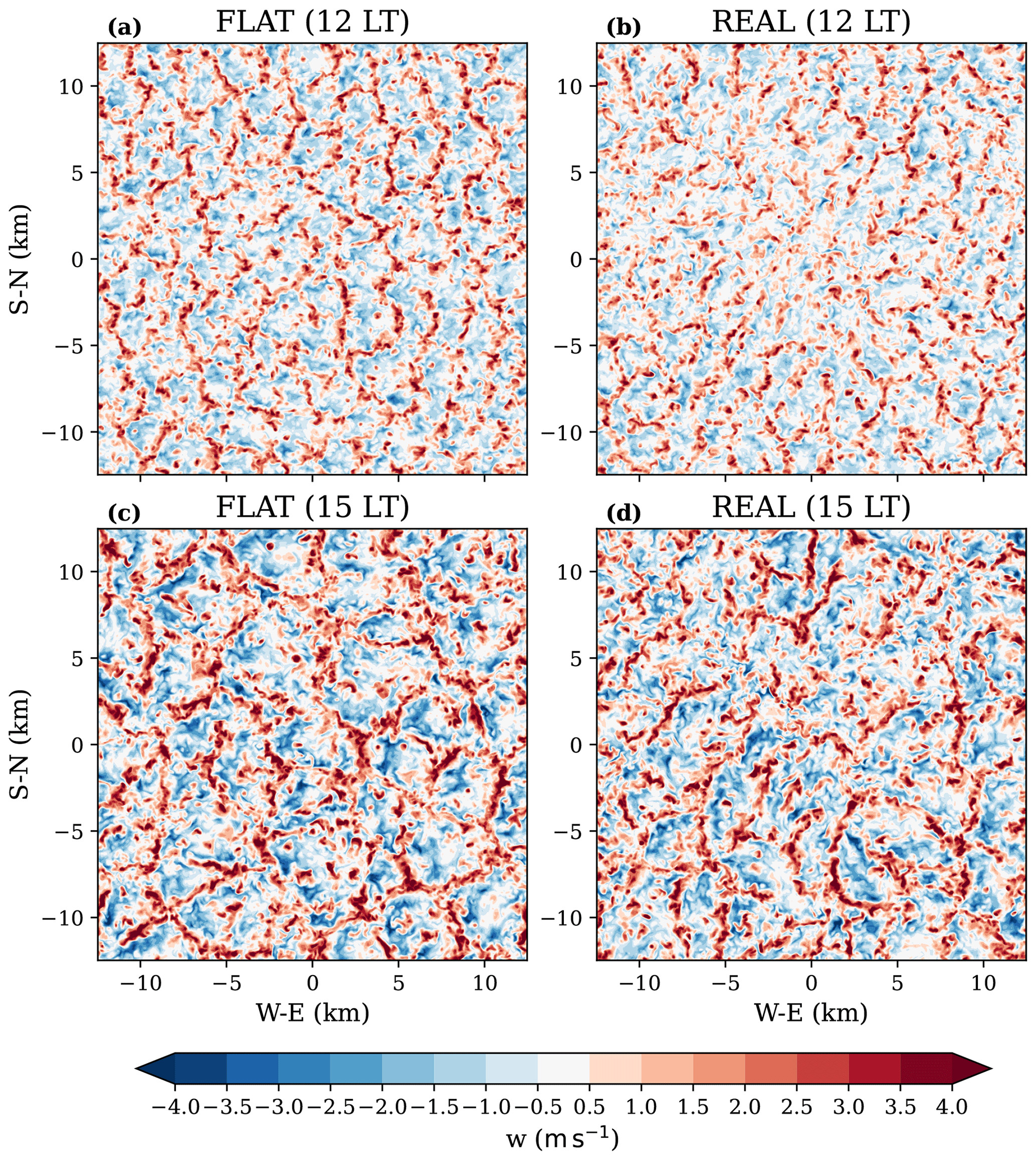
Figure 4 shows the instantaneous turbulent flow field in terms of the vertical velocity perturbation w^′ at 15:00 LT. The simulations share identical surface sensible heat fluxes and initial conditions, which leads to broadly similar turbulent structures across all cases. In the horizontal cross-sections (Fig. 4a–d) the turbulent field exhibits an irregular cellular pattern, with eddy structures ranging from a few hundred meters to over 5 km. In FLAT and REAL, the eddies are more or less randomly distributed throughout the domain, consistent with the prescribed homogeneous surface sensible heat flux. REALu10 and FLATu10 (Fig. 4c, d, g, and h) have slightly larger and more elongated horizontal eddy structures.

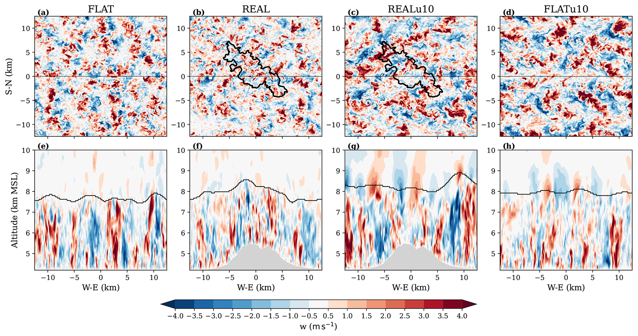
Figure 4 As in Fig. 3, but for the vertical velocity perturbation w^′ at 15:00 LT.

In addition to horizontal sections shown in Fig. 4, we examined instantaneous vertical velocity perturbation fields at lower levels (see Appendix C). At these heights (500 m a.g.l.), the turbulent structures appear as irregular, fine-scale cells. They are in contrast to the flow at 6 km a.m.s.l., which has larger, more coherent eddies and characteristic of fully developed convection.

3.3 Turbulence and Mixing

We examine turbulence intensity in terms of turbulence kinetic energy (TKE),

$$\begin{array}{}\text{(5)}& \text{TKE}={\displaystyle \frac{\mathrm{1}}{\mathrm{2}}}\stackrel{\mathrm{‾}}{({u^{\prime }}^{\mathrm{2}}+{v^{\prime }}^{\mathrm{2}}+{w^{\prime }}^{\mathrm{2}})},\end{array}$$

where $\stackrel{\mathrm{‾}}{u^{\mathrm{2}}},\stackrel{\mathrm{‾}}{v^{\mathrm{2}}},\stackrel{\mathrm{‾}}{w^{\mathrm{2}}}$ are given in Eq. (4):

$$\begin{array}{}\text{(6)}& \begin{array}{rl}{\displaystyle }\stackrel{\mathrm{‾}}{{u^{\prime }}^{\mathrm{2}}}& {\displaystyle }=\stackrel{\mathrm{‾}}{u^{\mathrm{2}}}-{\stackrel{\mathrm{‾}}{u}}^{\mathrm{2}}\\ {\displaystyle }\stackrel{\mathrm{‾}}{{v^{\prime }}^{\mathrm{2}}}& {\displaystyle }=\stackrel{\mathrm{‾}}{v^{\mathrm{2}}}-{\stackrel{\mathrm{‾}}{v}}^{\mathrm{2}}\\ {\displaystyle }\stackrel{\mathrm{‾}}{{w^{\prime }}^{\mathrm{2}}}& {\displaystyle }=\stackrel{\mathrm{‾}}{w^{\mathrm{2}}}-{\stackrel{\mathrm{‾}}{w}}^{\mathrm{2}}\end{array}\end{array}$$

During the day, vigorous turbulence efficiently mixes heat, momentum, and scalars, producing a well-developed CBL. At midday (15:00 LT), the TKE profiles of FLAT and REAL are similar, while the shear cases (REALu10 and FLATu10) show systematically higher values throughout and above the ABL (Fig. 5a). Since all runs start from identical conditions, this enhancement is expected: the added wind shear directly contributes to turbulence shear production (Fig. 5b). An increased TKE above the ABL, particularly in REALu10, also reflects weak gravity-wave activity generated by overshooting thermals over the ridge. Such waves are a physically expected response in a deeply convective, weakly stratified environment and do not materially affect the diagnosed ABL structure. Shear also organizes turbulence into roll structures, in contrast to the isolated plumes seen in the no-shear cases (see REAL and FLAT in Fig. 6).

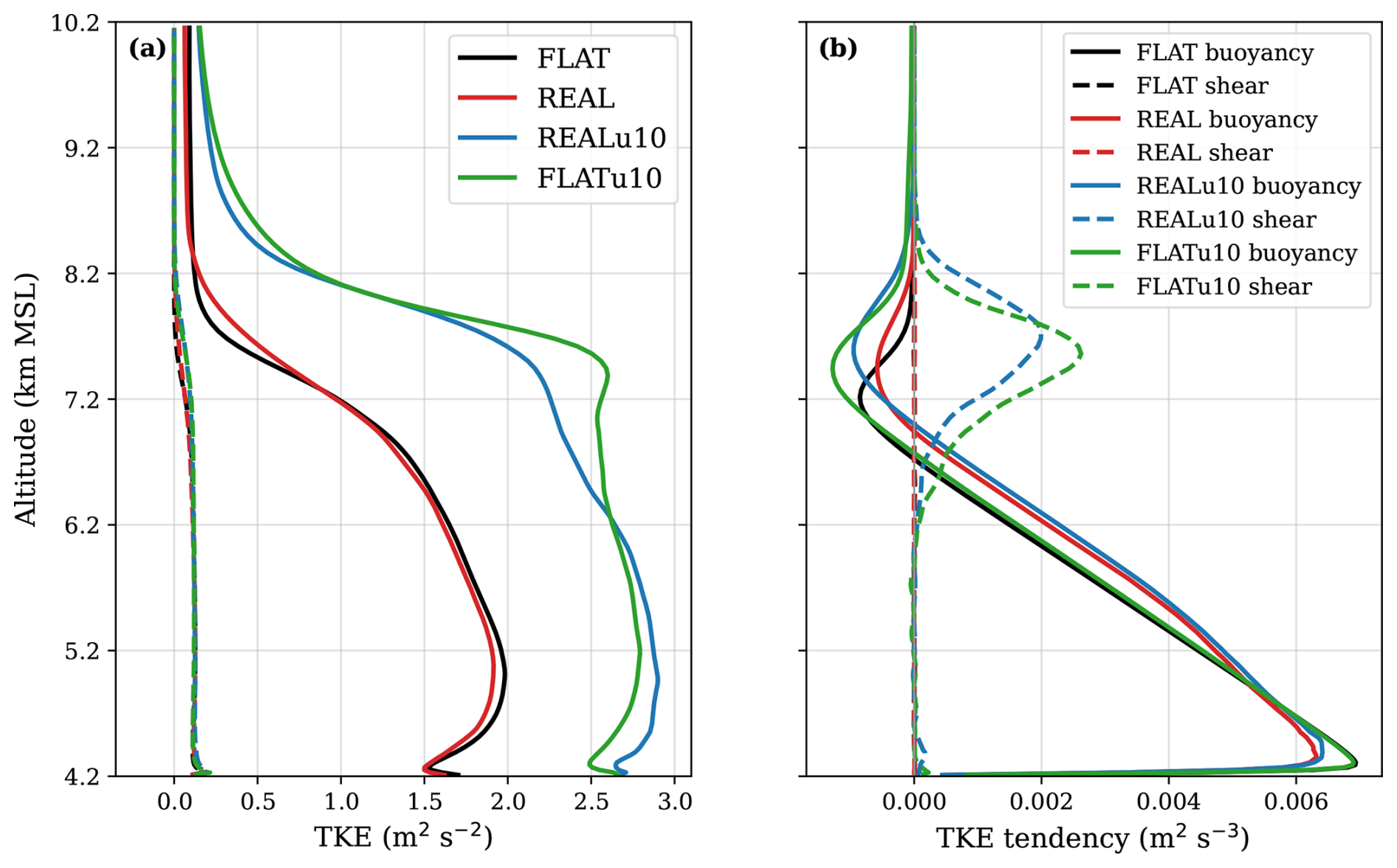
Figure 5 Mean vertical profiles at 15:00 LT on interpolated horizontal surfaces of (a) resolved and subgrid-scale TKE (solid and dashed lines, respectively), and (b) buoyancy production (solid lines) and shear production (dashed lines).

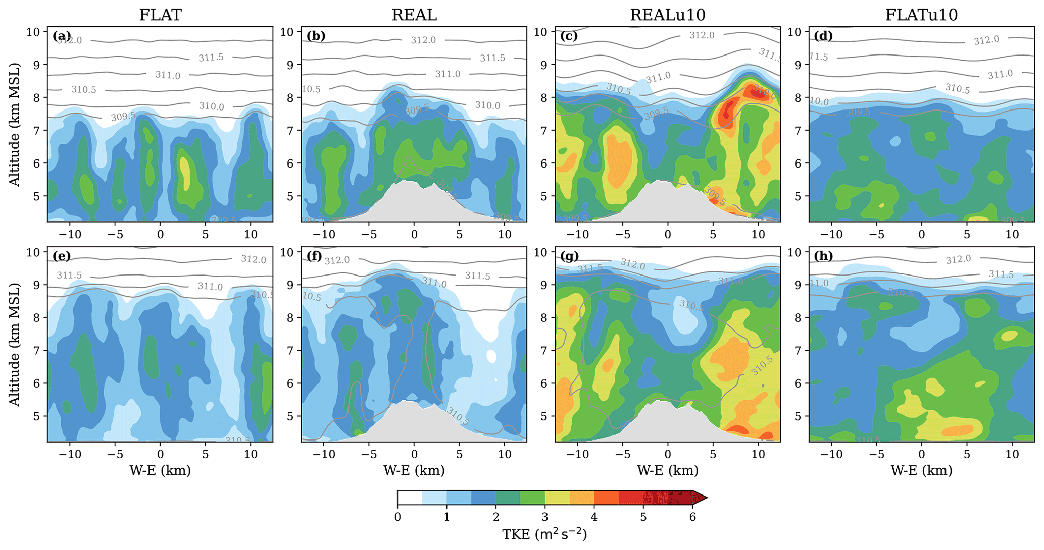
Figure 6 Vertical cross-sections of resolved TKE at 15:00 LT (a–c) and 19:00 LT (d–f), with $\stackrel{\mathrm{‾}}{\mathit{\theta }}$ in gray contours.

Between 15:00 and 19:00 LT, turbulence is sustained and convective eddies deepen in all experiments (Fig. 6e–h). By 19:00 LT, each case develops a very deep, well-mixed boundary layer. An important distinction emerges in the late afternoon: despite the decline in surface sensible heat flux, TKE does not decay as quickly as in a typical CBL at lower altitudes, most notably in the REALu10 case. This sustained turbulence is consistent with the weak static stability in our simulations, under which mechanically and thermally driven production can maintain elevated TKE values even as the surface forcing weakens. Whereas TKE in classic CBLs normally peaks in mid-afternoon and then decreases as buoyant production diminishes (see, e.g., Stull, 1988), the behaviour here instead indicates persistent thermally driven circulations under weak upper-level stability, consistent with the atmospheric structure described by Chen et al. (2016).

Terrain plays a clear role in shaping turbulence. In FLAT (Fig. 6a and e), TKE exhibits the classic CBL structure, with maxima concentrated in the middle of the mixed layer. In REAL (Fig. 6b and f), terrain heterogeneity anchors convective eddies to slopes, producing a more continuous turbulent layer above the mountain that extends above 9 km a.m.s.l. by 19:00 LT.

The effect of added shear (FLATu10) and terrain forcing (REALu10) further amplifies turbulence and promotes vertical TKE growth (Figs. 5a and 6c, d, g, and h). The turbulent structures are also more spatially homogeneous than in FLAT and REAL.

3.4 Passive tracers and ABL height Diagnosis

By midday, convective turbulence mixes the surface-based tracer within the growing boundary layer, producing a well-mixed state (Fig. 7). Columns of elevated tracer concentration coincide with persistent updraft cores (Fig. 3), especially over complex terrain where quasi-stationary thermals continuously draw tracers upward. The localized tracer maxima and uneven mixing are more pronounced in REAL (second column in Fig. 7) than in FLAT (first column), reflecting the orographic influence. In REALu10 and FLATu10, the added shear produces more homogeneous horizontal tracer fields (third and fourth column in Fig. 7) because of the shear-organized rolls (Fig. 6), leading to more uniform mixing. The vertical tracer extent in Fig. 7 provides a clear marker of the mixing depth, corresponding closely to turbulence maxima (Fig. 6) and thermal perturbations (Fig. 4). In REAL, tracer and turbulence extend higher over the ridge, while in REALu10 the tracer reaches greater heights over adjacent flat areas, consistent with shear-enhanced mixing. Entrainment from aloft further highlights these differences: in REAL, upper-level tracer mixes downward by 15:00 LT along the mountain flanks, whereas in FLAT entrainment is delayed until 17:00–19:00 LT and occurs more sporadically (Fig. 7i and m). In contrast, REALu10 and FLATu10 achieve more domain-wide and uniform entrainment and show the strongest entrainment fraction at 19:00 LT (Fig. 7m–p).

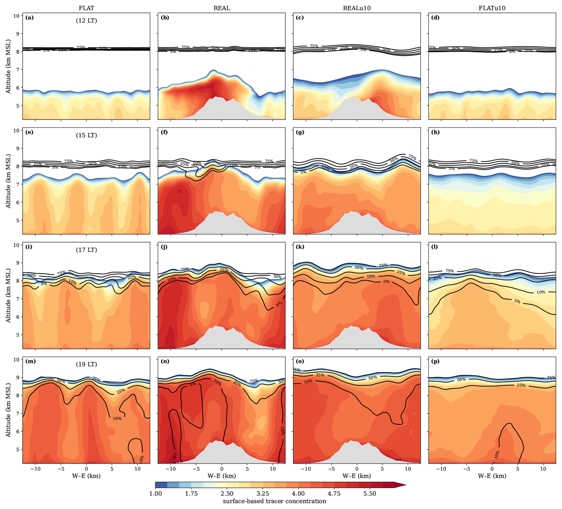
Figure 7 Vertical cross-sections of ensemble-mean surface-based (shading) and upper-level (black contours) passive tracers for the FLAT (left), REAL (middle), and REALu10 (right) experiments, shown every hour from 11:00 to 19:00 LT (rows). Surface-based tracer concentrations are shown as $\mathrm{kg}{\mathrm{kg}}^{-\mathrm{1}}\times {\mathrm{10}}^{\mathrm{4}}$; the scaling by 10⁴ is applied for readability and does not correspond to any specific chemical species. Shading for the surface-based tracer is plotted only where concentrations are at least 10 % of the domain-mean ABL tracer concentration to highlight the most pronounced features. The upper-level tracer contour lines are shown in percentages of the initial concentration (c_0,upper).

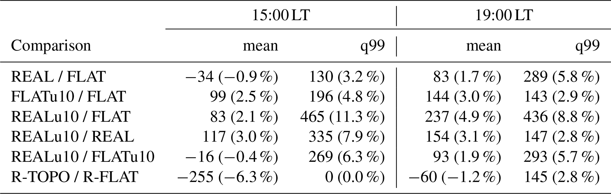
Tracer-based profiles and diagnosed ABL heights (Fig. 8) confirm these contrasts. As shown in Fig. 8a and b, orography alone has only a small influence on the domain-mean ABL height (REAL–FLAT). By contrast, adding shear over flat terrain (FLATu10–FLAT) deepens the mean ABL height by roughly 12 % at 15:00 LT and 5 % at 19:00 LT, and similar increases occur when shear is added over real terrain (REALu10–REAL). The combined effect relative to the FLAT baseline (REALu10–FLAT) is about 13 % at 15:00 LT and 7 % at 19:00 LT, indicating that shear is the primary driver of domain-mean deepening, with orography providing a smaller but positive secondary contribution.

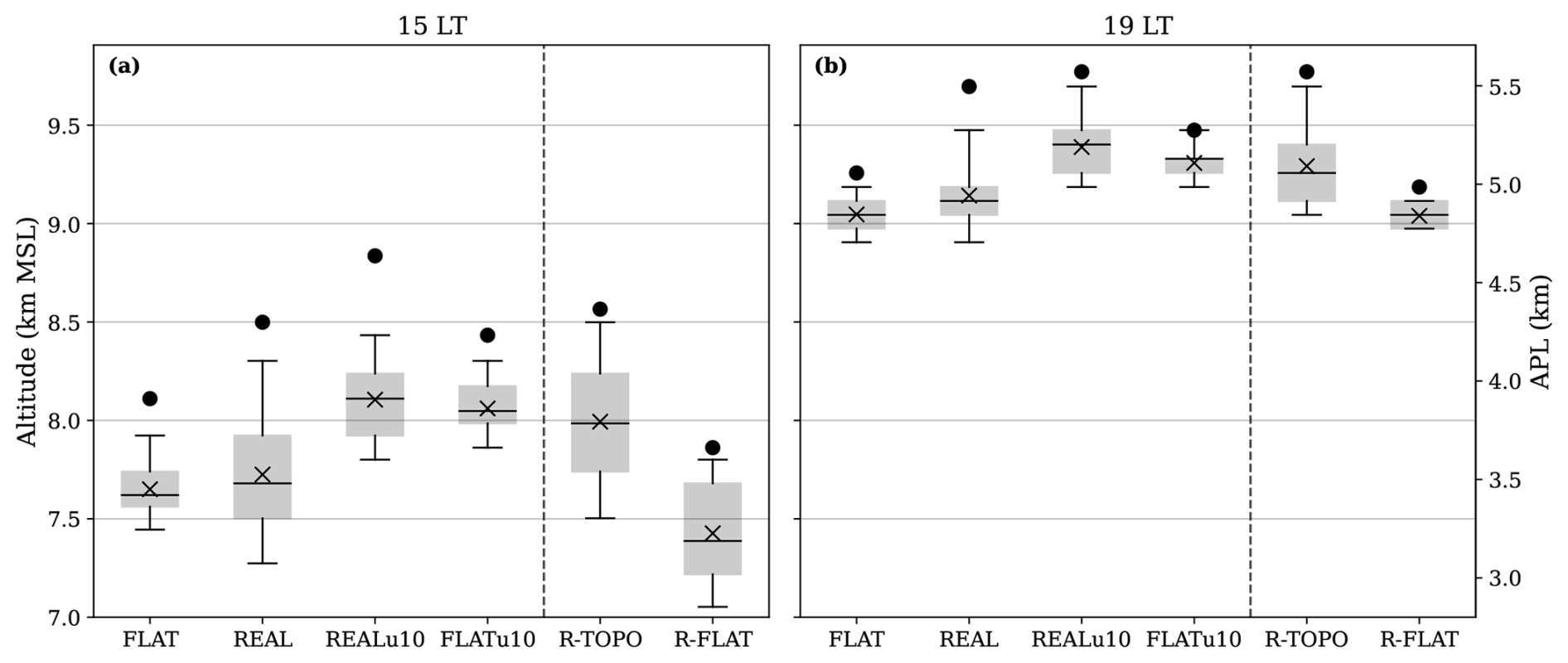
Figure 8 Horizontal variability of the ABL height diagnosed from the ensemble-averaged surface-based tracer at (a) 15:00 and (b) 19:00 LT. For each experiment, box-whisker diagrams show the 25th–75th percentile range, whiskers the 5th–95th percentiles, crosses the mean, and circles the 99th percentile. Heights are shown in  km m.s.l. (left axis) and in km APL (right axis). A vertical dashed line separates the four full-domain experiments from the two REAL subdomains (R-TOPO and R-FLAT).

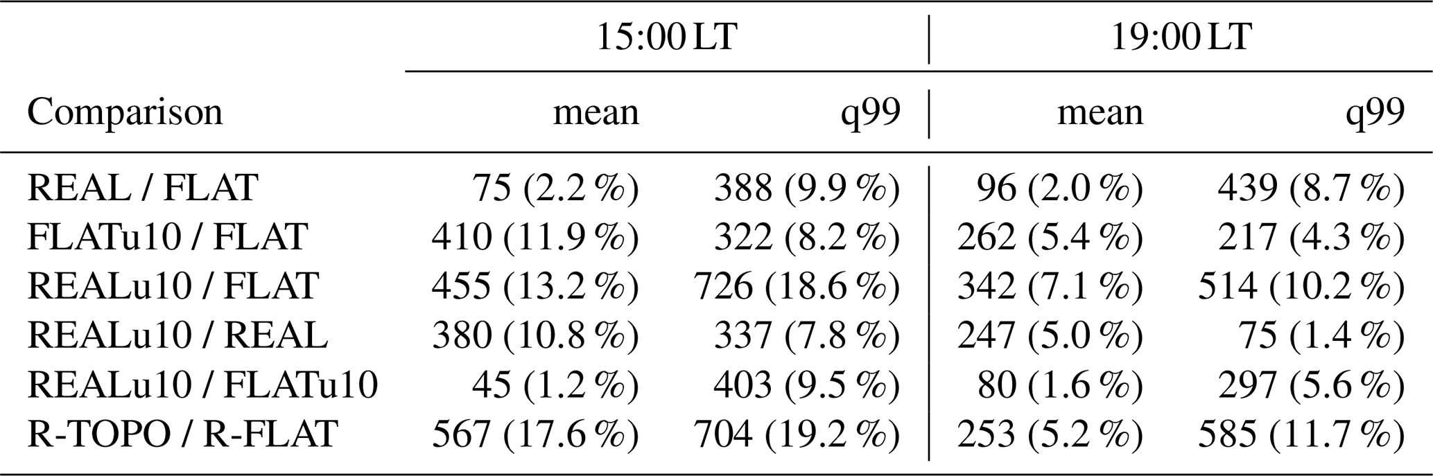
The upper tail of the ABL height distribution (99th percentile in Fig. 8) reveals a much stronger orographic imprint. At the domain scale, REAL exceeds FLAT by about 10 % at 15:00 and 19:00 LT in the 99th percentile, whereas the shear-induced increases (FLATu10–FLAT; REALu10–REAL) are smaller, especially at 19:00 LT. The strongest orographic impact, however, appears in the REAL subdomains: at 15:00 LT the R-TOPO mean ABL height exceeds R-FLAT by about 18 %, and the 99th percentile is almost 20 % higher. By 19:00 LT, the differences decrease but remain distinct (5 % for mean; nearly 12 % for 99th percentile). Thus, while domain-mean metrics are dominated by shear, small-scale orography substantially amplifies the deepest convective columns, especially over the mountain, with implications for upper-level tracer exchange. These quantitative values are summarized in Table 2.

Table 2 Differences in diagnosed ABL height between experiments at 15:00 LT and 19:00 LT. Values denote the difference in metres APL, and the relative difference in percent (relative to the lower experiment in each pair) in parentheses. Columns labelled “mean” refer to domain-mean ABL height; columns labelled “q99” refer to the 99th percentile.

Although these results show that the ABL height (in m MSL) increases over the mountain, the ABL depth (in m a.g.l.) is actually shallower there. Figure 9 clarifies this distinction by relating the diagnosed ABL height to the underlying terrain elevation. Figure 9b shows that ABL heights increase with elevation in REAL, consistent with elevated tracer layers and terrain-anchored thermals. However, Fig. 9a shows that the ABL depth (a.g.l.) decreases with increasing terrain height, particularly in REALu10, because the ridge raises the reference plane from which depth is measured. This demonstrates that the influence of small-scale orography is more nuanced than implied by height (MSL) alone: the ABL can be deeper in an absolute sense over the mountains while simultaneously being shallower relative to the local ground surface.

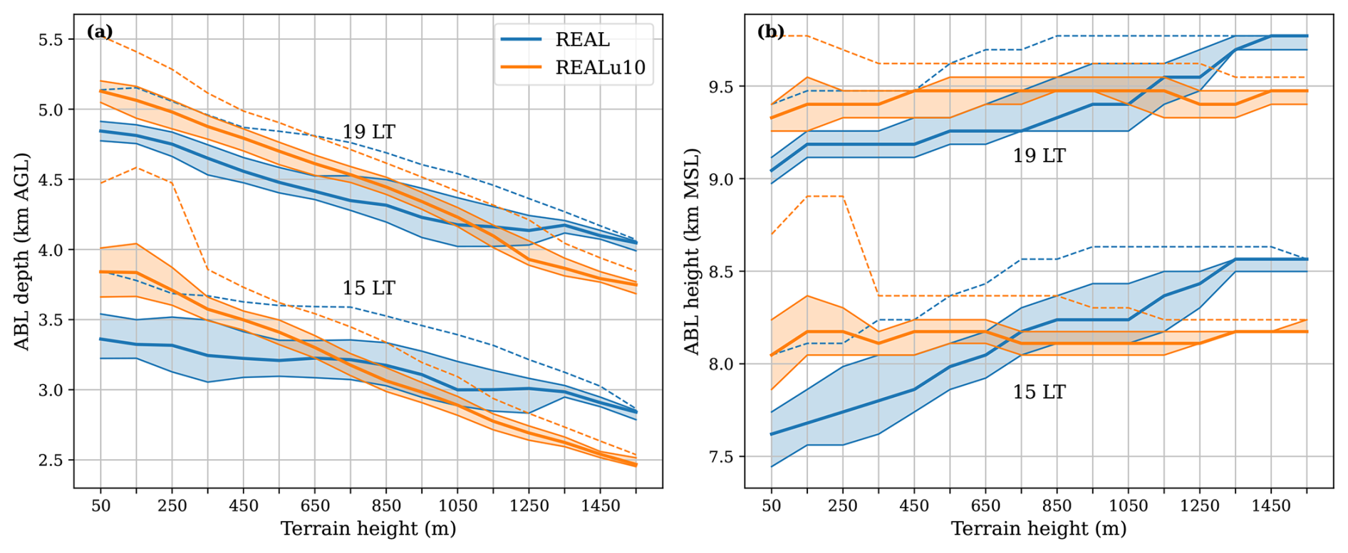
Figure 9 (a) ABL depth in km a.g.l. and (b) ABL height in  km m.s.l. as a function of underlying terrain elevation (m APL) for REAL and REALu10 at 15:00 and 19:00 LT. Terrain is grouped into 100 m bins. For each terrain bin, solid curves denote the median, shaded bands the 25–75th percentiles, and dashed lines the 99th percentiles.

Finally, our tracer-based ABL height detection method (described in Sect. 2.3.2) proved robust: applying a 5 % concentration threshold yielded consistent and physically meaningful height distributions that aligned well with turbulence features (Fig. 6). Importantly, similar distributions were obtained whether using instantaneous fields, time-averaged data, or ensemble means, indicating that the method is not overly sensitive to the choice of averaging.

4 Conclusions

In this study, we performed high-resolution LES experiments under idealized dry conditions to quantify the impact of small-scale orography on the development of an exceptionally deep convective boundary layer (CBL) over the western Tibetan Plateau. We compared simulations with realistic complex terrain (REAL; an isolated mesoscale mountain embedded in an elevated plain) and with a horizontally uniform plateau (FLAT), both initialized at 4.2 km elevation. Two additional simulations included a steady upper-level background wind of 10 m s⁻¹ over flat (FLATu10) and realistic terrain (REALu10), allowing us to separate and combine the effects of small-scale orography and vertical wind shear.

Small-scale orography enhances boundary-layer growth locally by anchoring thermals over slopes and ridge tops. In the early afternoon, ABL heights over the ridge exceed those over adjacent flat areas by up to 20 % in the upper percentiles, while domain-mean differences between REAL and FLAT remain comparatively modest (Table 2). Introducing upper-level shear deepens the boundary layer more uniformly across the domain: shear-driven roll vortices in FLATu10 and REALu10 organize and sustain turbulence, yielding mean ABL heights that are roughly 10 %–15 % deeper than in the corresponding no-shear cases at 15:00 LT, and still noticeably deeper by 19:00 LT. By late afternoon, the combined terrain and shear effects in REALu10 produce the deepest and most laterally uniform ABL, with diagnosed heights approaching 9.4 km a.m.s.l..

Our passive-tracer analysis shows that terrain and shear act through distinct but complementary mechanisms. Orography locks the strongest updrafts to the ridge, intensifying TKE and tracer plumes locally and accelerating entrainment along slopes and ridge tops, whereas shear organizes convection into longitudinal rolls that enhance domain-wide mixing efficiency. Tracer-based ABL height diagnostics and percentile statistics (Fig. 8 and Table 2) highlight this complementarity: shear is the primary driver of the increase in domain-mean ABL height, while small-scale orography exerts a disproportionate influence on the upper tail of the ABL height distribution. In particular, the REAL subdomain over the ridge (R-TOPO) shows substantially higher mean and 99th-percentile ABL heights than the adjacent flat subdomain (R-FLAT), further showing how a relatively small fraction of the domain can have much deeper convective columns.

An important nuance emerging from our analysis is the distinction between ABL height above mean sea level and ABL depth above the local surface. Figure 9 shows that, although ABL heights (m MSL) increase with terrain elevation (and are highest over the ridge in REAL) the ABL depth (m AGL) actually decreases with terrain height, especially in REALu10. In other words, the CBL over the mountain is higher in absolute terms but shallower relative to the underlying terrain than over the surrounding plateau. This emphasizes that local orographic impacts on the CBL cannot be inferred from heights MSL alone; both the vertical extent above the surface and the distribution of terrain elevations within the domain matter for interpreting vertical exchange and tracer transport.

The extreme ABL depths reproduced in our simulations are consistent with radiosonde observations over the Tibetan Plateau, which report CBLs of up to 5 km a.g.l. (∼9.4 km a.m.s.l.) under fair-weather winter conditions (Chen et al., 2013, 2016). Our results reinforce the importance of weak stratification aloft and strong surface heating as prerequisites for such development, and the diagnosed entrainment of upper-level tracer aligns with observed pathways for stratospheric ozone to influence surface air (Yin et al., 2023). The contrasting tracer distributions between REAL and REALu10 are also consistent with terrain-anchored plumes and shear-driven rolls identified in previous modeling studies (Lai et al., 2021). More broadly, our findings support growing evidence that unresolved orography biases ABL representation and that explicitly resolving terrain-induced circulations can improve realism in weather and climate models (Wagner et al., 2014; Guo et al., 2021; Poll et al., 2022; Goger et al., 2022).

Our configuration is intentionally idealized, excluding moist convection, clouds, and synoptic variability, in order to isolate the roles of orography and shear. While this strengthens attribution, it also limits direct comparability with real cases. The terrain in our REAL experiments consists of a single mesoscale mountain of order 1 km relief embedded in an elevated plain; we have not explored systematic variations in mountain height, horizontal scale, or the presence of multiple ridges and valleys. The scale-dependence of our results remains an open question and should be addressed in future LES studies. Likewise, our simulations reflect the specific large-scale environment of the selected day, characterized by unusually weak free-tropospheric stability that favors extreme CBL growth. Future work should test the robustness of our conclusions under more realistic forcing (e.g., TIPEX-III field days; Che and Zhao, 2021) and across a broader range of stratification and background-flow regimes (cf. Singh et al., 2024).

Finally, our tracer-based ABL height diagnostic, which uses a 5 % threshold relative to the column-mean mixed-layer tracer concentration (Sect. 2.3.2), proved robust and physically interpretable. The resulting ABL height distributions align closely with features in the turbulence and temperature fields (Figs. 4 and 6), and they are relatively insensitive to whether instantaneous, time-averaged, or ensemble-mean tracer fields are used. Overall, our results show that small-scale orography sustains and organizes turbulence over the Tibetan Plateau, thereby enhancing boundary-layer mixing and contributing to the exceptionally deep ABLs that form under weak free-tropospheric stability. Because these terrain-driven processes are subgrid-scale in most weather and climate models, better representation of orographic circulations and shear–terrain interactions is essential for realistically simulating vertical transport of heat, momentum, and trace species, and for improving forecasts and climate projections in mountainous regions.

Appendix A: Comparison Between Two ABL height Diagnosis Methods

To evaluate the robustness of our tracer-based boundary layer height (ABL height) diagnosis, we compare it against a commonly used alternative: the parcel method (Duncan et al., 2022).

The TKE threshold method was initially considered, but ultimately excluded from the analysis. It exhibited high spatial and temporal variability and required sensitive tuning of threshold values. Despite such tuning efforts, it consistently produced less physically plausible results compared to the parcel method and tracer-based approach.

Figure A1 shows a comparison between the tracer-based ABL height and the parcel ABL height at 15:00 and 19:00 LT, with the parcel method using ensemble averaged potential temperatures ($\stackrel{\mathrm{‾}}{\mathit{\theta }}$). The parcel method diagnoses that the median and mean ABL height values exceed those from the tracer method by a substantial margin at 15:00 LT (apart from REALu10 and R-TOPO). While the initial rise is faster, the ABL heights at 19:00 LT are comparable. The differences between the distributions of ABL heights between the experiments are lesser in the parcel method (see Table A1), than in the tracer method (Table 2). On a closer look, it could be due to the ABL height at 09:00 LT being almost 1 km higher than in the tracer method, since the surface passive tracer starts at zero. The difference between mean ABL heights in FLAT and REAL are also very modest, as well as differences in the 99th-percentiles.

The tracer method we used better captures the integrated effects of turbulent mixing and entrainment and avoids overestimation in regions with strong surface heterogeneity. While it does not capture sharp inversion layers as directly as temperature-based methods, its stability and sensitivity to vertical transport make it well-suited for diagnosing the evolving CBL in high-altitude terrain.

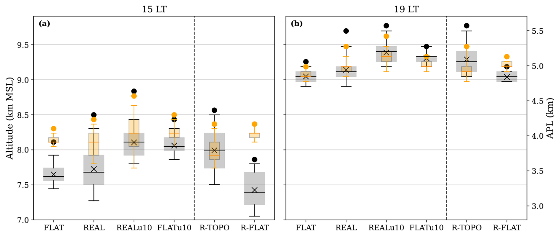
Figure A1 As in Fig. 8, but comparing the tracer ABL height to the parcel ABL height method (light orange boxes). The mean parcel ABL height is not marked.

Table A1 As in Table 2, but based on ABL heights diagnosed with the parcel method. Values denote the difference in metres APL, and the relative difference in percent (relative to the lower experiment in each pair) in parentheses.

Appendix B: Super-Gaussian Tapering of the Lateral Boundaries

To avoid sharp elevation changes at the lateral boundaries and to reduce spurious wave reflections, the realistic terrain (REAL) is smoothly tapered toward the minimum elevation using a two-dimensional super-Gaussian mask. The mask is centered on the main ridge and defined in an elliptical coordinate system aligned with the dominant terrain orientation.

Let (x_c,y_c) denote the center of the ellipse, and let a and b be the semi-major and semi-minor axes, respectively. We first rotate the horizontal coordinates by an angle θ (measured counterclockwise from the x-axis),

$$\begin{array}{}\text{(B1)}& {\displaystyle }{x}^{\prime }& {\displaystyle }=(x-x_{\mathrm{c}})\cos \mathit{\theta }+(y-y_{\mathrm{c}})\sin \mathit{\theta },\text{(B2)}& {\displaystyle }{y}^{\prime }& {\displaystyle }=-(x-x_{\mathrm{c}})\sin \mathit{\theta }+(y-y_{\mathrm{c}})\cos \mathit{\theta },\end{array}$$

and then define the super-Gaussian mask as

$$\begin{array}{}\text{(B3)}& M(x,y)=\exp \left[-\left({\displaystyle \frac{{x^{\prime }}^n}{\mathrm{2}{a}^n}}+{\displaystyle \frac{{y^{\prime }}^n}{\mathrm{2}{b}^n}}\right)\right],\end{array}$$

where n is the order of the super-Gaussian. In the present study, we use n=4, a=9 km, b=4.8 km, and θ=330°, which produces an approximately flat interior plateau region and a gradual decay toward the domain edges.

The tapered elevation field is then constructed as

$$\begin{array}{}\text{(B4)}& h_{\text{taper}}(x,y)=h_{\text{min}}+M(x,y)\left(h_{\text{raw}}\right(x,y)-h_{\text{min}}),\end{array}$$

where h_raw(x,y) is the interpolated SRTM topography on the CM1 grid and h_min is the minimum elevation within the domain. This formulation ensures that

$$M\approx \mathrm{1}\text{in the interior (ridge–valley region)}\Rightarrow h_{\text{taper}}\approx h_{\text{raw}},$$

while

$$M\to \mathrm{0}\text{near the lateral boundaries}\Rightarrow h_{\text{taper}}\to h_{\text{min}},$$

thus providing a smooth lateral transition from realistic terrain to a uniform base elevation over the outer 4 km of the domain.

Appendix C: Instantaneous flow patterns at lower heights

Figure C1 shows horizontal cross-sections of instantaneous vertical velocity perturbations at 500 m a.g.l. for FLAT and REAL at 12:00 and 15:00 LT. At 12:00 LT, the flow is characterized by relatively small (2 km), cellular updraft–downdraft structures typical of an early CBL (2–4 km depth). By 15:00 LT, these cells have merged into fewer, larger (5 km) structures, reflecting the growth of the convective length scale as the ABL deepens.

Figure C1 As in Fig. 4a–b, but for 500 m a.g.l. at 12:00 and 15:00 LT, for FLAT and REAL.