Strong control of the stratocumulus-to-cumulus transition time by aerosol: analysis of the joint roles of several cloud-controlling factors using Gaussian process emulation

Stratocumulus-to-cumulus transitions are driven primarily by increasing sea-surface temperatures, with additional contributions from numerous interacting cloud-controlling factors. Understanding these interactions is important for improving the accuracy of cloud responses to changes in climate and other environmental factors in global climate models. Many studies have found lower-tropospheric stability dictates the transition time, while aerosol-focused studies found that aerosol concentration plays a key role via the drizzle-depletion mechanism. We consider the role of aerosol together with several other cloud-controlling factors representing a selection of the wider environmental conditions that affect drizzle in a clean to moderately polluted environment. A 34-member perturbed parameter ensemble of idealised large-eddy simulations with 2-moment cloud microphysics is used to train Gaussian process emulators (statistical representations) of the relationships between the factors and two properties of the transition: transition temporal length and average rain water path. We base the ensemble around a composite of trajectories in the Northeastern Pacific during summer. Using these emulators, parameter space can be densely sampled to visualise the joint and individual effects of the factors on the transition properties. We find that in the low-aerosol regime (< 200 cm⁻³) the transition time is most strongly affected by the aerosol concentration out of the factors considered here. Fast transitions, under 40 h, occur in this regime with high mean rain water path, which is consistent with a drizzle-depletion effect. In the high-aerosol regime, the inversion strength becomes more important than the aerosol concentration through the inversion's effect on entrainment and the deepening-warming decoupling mechanism.

1 Introduction

Stratocumulus-to-cumulus transitions occur in the east of major ocean basins when stratocumulus decks are advected towards the equator across increasingly warmer sea-surface temperatures (SST) (Klein and Hartmann, 1993; Albrecht et al., 1995). There is a large decrease in cloud fraction, albedo and cloud radiative effect as the cloud deck transitions to cumulus. The stratocumulus-to-cumulus transition is governed by many cloud-controlling factors, whose contributions are still an area of active research. Uncertain processes lead to poor parameterisations in global climate models (GCMs) so transitions are not captured well, which creates large uncertainties in simulated cloud properties and their responses to the warming climate (Bony and Dufresne, 2005; Teixeira et al., 2011; Eastman et al., 2021). Low clouds in the subtropics have a cooling effect on the planet, and since GCMs project a future decrease in subtropical cloud fraction, that cooling effect will be weakened, amplifying warming, and contributing to a positive cloud feedback effect (Bretherton, 2015; Ceppi et al., 2017; Nuijens and Siebesma, 2019). Further process understanding of cloud transitions will improve their representation in GCMs and reduce the uncertainty surrounding cloud adjustments and feedbacks.

The typical transition mechanism, termed deepening-warming decoupling, has been determined through observational studies (Paluch and Lenschow, 1991; Bretherton and Pincus, 1995; Bretherton et al., 1995; Martin et al., 1995; Wang and Lenschow, 1995; Klein et al., 1995; de Roode and Duynkerke, 1996; Pincus et al., 1997) and high-resolution modelling (Krueger et al., 1995; Wyant et al., 1997; Bretherton and Wyant, 1997; Svensson et al., 2000). It describes how increasing SSTs cause the boundary layer turbulence to be increasingly driven by surface fluxes that deepen the boundary layer and enhance the entrainment of warm and dry air at cloud top. As the boundary layer deepens, mixing throughout the full layer can no longer be sustained as the sub-cloud air cools and moistens, so the boundary layer decouples into a stratocumulus cloud layer and a surface-coupled sub-cloud layer (Bretherton and Wyant, 1997). Once decoupled, the moisture is supplied to the stratocumulus by cumulus plumes emerging from the sub-cloud layer, rather than eddies driven by cloud-top radiative cooling and surface fluxes. In this cumulus-under-stratocumulus stage, the plumes at first provide moisture and turbulence to the stratocumulus layer, but more-energetic plumes overshoot and vigorous mixing eventually dissipates the stratocumulus cloud resulting in a field of cumulus.

The role of drizzle in the transition has historically been inconsistent between studies (Miller and Albrecht, 1995; Wang, 1993; Pincus et al., 1997; Svensson et al., 2000). Several modelling studies have found that drizzle plays a small role compared to other cloud-controlling factors (Sandu and Stevens, 2011; McGibbon and Bretherton, 2017; Blossey et al., 2021). For example, Sandu and Stevens (2011) perturbed cloud-controlling factors in a large-eddy simulation (LES) of a composite case derived from thousands of trajectories in the North East Pacific (Sandu et al., 2010). Reducing cloud droplet number concentration from 100 to 33 cm⁻³ allowed precipitation to form earlier and limited boundary layer recovery from decoupling through moistening and cooling the sub-cloud layer and depleting the cloud layer of water. The cloud did break up faster, but the initial strength of the temperature inversion capping the boundary layer had a stronger control on the timing of the breakup. However, as in many LES studies, a fixed droplet number was used, while Yamaguchi et al. (2017) showed that aerosol collision-coalescence processes are required to represent droplet depletion. Chun et al. (2025) included aerosol processing and found that aerosol injection suppressed precipitation, however they found the aerosol effect on the transition is overestimated where large-scale circulation adjustments are ignored.

Including collision-coalescence processes in LES models ensures there is a feedback between the reduction of droplets as they collide and the reduction in aerosol number concentration, which then further reduces cloud droplet number. Using an LES model with a microphysics scheme that included this processing, Yamaguchi et al. (2017) found that a fast transition mechanism is initiated in a low-aerosol environment. They proposed that drizzle droplets are formed in cumulus plumes and strong updrafts carry them to the stratocumulus layer where they enhance drizzle production because they are larger than the stratocumulus cloud droplets, and therefore more efficient collectors. Through collision-coalescence and wet scavenging, the droplet number and aerosol concentrations are reduced leading to even heavier drizzle, more reduction and a runaway feedback. Using the same model for a different case, Diamond et al. (2022) also found a rapid reduction in cloud fraction through drizzle depletion in low aerosol conditions, with an end state closer to open-cellular organisation rather than cumulus. Erfani et al. (2022) used single-mode bulk microphysics that included aerosol processing within cloud droplets, and also found precipitation to be a key driver of the transition. These studies do not fully consider the effect of aerosol concentration in the context of other cloud-controlling factors: Diamond et al. (2022) perturbed some large-scale forcings but with a focus on smoke effects, while the trajectories in Erfani et al. (2022) had very different initial conditions but cover only two extreme cases.

Observations from ships and satellites, along with reanalysis data, provide wider meteorological context (e.g. Mauger and Norris, 2010), but they have not shown clear evidence of a rapid transition to cumulus by a drizzle-depletion mechanism (Pincus et al., 1997; Zhou et al., 2015; Brendecke et al., 2021). Eastman and Wood (2016) analysed Lagrangian trajectories from satellite data to study how boundary layer depth, the inversion strength and precipitation affect cloud evolution. Deep boundary layers and weak inversions tended more towards cloud breakup, but precipitation effects were less clear: in shallow boundary layers, precipitation sustained the cloud whereas in deep boundary layers it caused cloud breakup. Despite finding that increases in aerosol increased average cloud fraction, Christensen et al. (2020) also did not find precipitation or low aerosol to be a strong driver of cloud breakup. Eastman et al. (2022) assessed the difference between closed-cell stratocumulus that do and do not transition. Heavy precipitation was linked closely with a transition to open-cell stratocumulus, but the transition to a cumulus state is more likely caused by excess entrainment at cloud top.

High-resolution model simulations of the transition have been limited to one-at-a-time perturbations, or only a few detailed trajectories, which sample only a few points in what is a multi-dimensional “parameter space” created by all the cloud-controlling factors. Sandu and Stevens (2011), van der Dussen et al. (2016), and Zheng et al. (2021) made large one-at-a-time perturbations to meteorological conditions, such as subsidence, droplet number, radiation and latent heat fluxes. LES model intercomparisons of the transition compared with observations highlight which structural differences create the largest disparities in replicating observed transitions (Bretherton et al., 1999; van der Dussen et al., 2013; de Roode et al., 2016). Small perturbations to initial conditions can represent different stages of the transition (Chung et al., 2012; Tsai and Wu, 2016; Bellon and Geoffroy, 2016), while simulating observed or computed trajectories with completely different sets of initial conditions produces very different transition characteristics (Goren et al., 2019; Blossey et al., 2021; Erfani et al., 2022). Within these studies, precipitation is found to have no effect or to slightly hasten the transition but it is not found to be a key driver. However, because these studies could only sample parameter space a few times, covariance between some meteorological factors may have been overlooked and so missing interactions between factors (Feingold et al., 2016).

Using machine learning, “emulators” can statistically represent the multi-dimensional relationship between a set of cloud-controlling factors (parameters) and a specific cloud property. The behaviour of complex cloud models can be efficiently sampled to create training data using a perturbed parameter ensemble (PPE) approach, where parameters are perturbed in combination, rather than one at a time. This method provides sufficient information with a sparse sampling of the multi-dimensional parameter space, which is ideal for emulating computationally expensive models. Gaussian process emulation works well with relatively few points compared to other machine learning methods (tens or hundreds as opposed to thousands) (O'Hagan, 2006). Once validated, the emulators can be used to fill the multi-dimensional parameter space with predictions. This dense sampling can then be used for sensitivity analysis to quantify the contributions from each factor to the variance in the property (Saltelli et al., 2000; Johnson et al., 2015; Wellmann et al., 2018, 2020) or to create response surfaces, which enable us to visualize non-linear joint effects of factors or the relationships between cloud states, e.g., Glassmeier et al. (2019) and Hoffmann et al. (2020). The PPE method with emulation is well suited to identifying distinct behaviour regimes in cloud models (e.g., Johnson et al., 2015; Sansom et al., 2024).

In this study we have used an LES model to create an ensemble of stratocumulus-to-cumulus transitions initiated with a wide range of meteorological conditions covering key cloud-controlling factors. We define “transition” as the time (in hours) taken to transition from the initial stratocumulus state to a cumulus state. Given the potential importance of drizzle formation, the ensemble also varies the dependence of cloud-to-rain autoconversion on the cloud droplet number concentration. Each of these perturbed factors has the potential to affect the characteristics of the transition, and in perturbing them simultaneously and in various combinations, we can learn how they jointly affect the transition. We then apply Gaussian process emulation to the PPE to create emulators of transition time and average rain water path. We address the following questions. (1) What combination of factors is most important in determining the transition time? (2) What combination of factors is most important in determining the drizzle amount, and how does drizzle affect the transition time? (3) Under what conditions might a drizzle-depletion mechanism occur?

2 Simulation and ensemble design

2.1 Model configuration

The PPE is based on the composite stratocumulus-to-cumulus transition case in Sandu and Stevens (2011). Sandu et al. (2010) computed thousands of forward and backward air parcel trajectories from areas of extensive cloud cover in the NE Pacific between May and October for 2002 to 2007. Boundary layer properties were retrieved over a six day period of advection from satellite data and meteorological reanalysis. Sandu et al. (2010) found that the climatological, or averaged, trajectory represented the key characteristics of the transition well. Sandu and Stevens (2011) developed this into a reference case for numerical simulation that represents a typical trajectory in the NE Pacific for June to August in 2006 and 2007 from a subset of trajectories for the three days in which the majority of the transition occurred. The meteorological state in this reference case is a good starting point for simulating a typical transition in the NE Pacific, from which we perturbed a range of cloud-controlling factors to explore variations in cloud behaviour.

The ensemble was simulated using the UK Met Office and National Environmental Research Council (NERC) LES model, called the MONC (Met Office/NERC Cloud) model (Dearden et al., 2018; Poku et al., 2021; Böing et al., 2019; Brown et al., 2020). The model solves a set of Boussinesq-type equations, using an anelastic approximation here, which is based on a reference potential temperature profile that depends only on height. The subgrid turbulence parameterization is an extension of the Smagorinsky-Lilly model and is based on that described in Brown et al. (1994). Version 0.9.0 of the Leeds-MONC Github repository was adapted for this study and released as version 0.9.1 (Denby et al., 2025). Here, MONC was coupled to the two-moment Cloud AeroSol Interaction Microphysics scheme (CASIM, version 6341: Shipway and Hill, 2012; Hill et al., 2015) and the Suite of Radiation Transfer Codes based on Edwards and Slingo (SOCRATES, version 1012: Edwards and Slingo, 1996).

CASIM is a two-moment bulk microphysics scheme that represents hydrometeors using gamma distributions for mass and number (Grosvenor et al., 2017; Field et al., 2023). Only warm-cloud processes (cloud liquid and rain) were used since ice processes are not part of the stratocumulus-to-cumulus transition in the NE Pacific. Simulations were initiated with soluble aerosol represented by prognostic mass and number concentrations in the Aitken and accumulation modes. The Aitken mode distribution has a standard deviation of 1.25 and a mean radius of 25 nm. The accumulation mode distribution has a standard deviation of 1.5 and a mean radius of 100 nm. The density of all aerosol particles was assumed to be 1500 kg m⁻³. All aerosol size modes were represented by a lognormal distribution. At saturation, the number of aerosol particles activated into cloud droplets was calculated using the scheme of Abdul-Razzak and Ghan (2000), and these activated aerosol were represented using a separate in-cloud aerosol prognostic. Aerosol material contained within droplets can grow through droplet collision and coalescence with the assumption that one aerosol particle was present in each droplet, and is returned to the appropriate aerosol size mode on evaporation of the cloud droplets (including the coarse mode). Accretion and autoconversion are represented by the Khairoutdinov and Kogan (2000) parameterization. Rain can evaporate in the subsaturated grid boxes, but aerosol is not returned to the size modes through this process.

Stratocumulus-to-cumulus transitions are often simulated in a Lagrangian style in which the domain moves with the advected cloudy air (Krueger et al., 1995; Sandu and Stevens, 2011; de Roode et al., 2016). As in other studies, we simulated the advection towards the equator by forcing the SSTs to increase over the course of the simulation. Wind profiles were retained to ensure appropriate ocean surface evaporation, but the model has periodic boundary conditions so the domain was always focused on the same cloud cell. The temperature and specific humidity profiles were allowed to evolve freely and the large-scale divergence was set to a constant value of 1.86 × 10⁻⁶ s⁻¹. The large-scale subsidence is calculated in the model as −Divergence × vertical height above sea level. Simulations were run for 3–4 d with a spin-up period of around an hour being discarded. The SST was increased by nearly 1.5 K per day, from 293.75 to 300.93 K, following Sandu and Stevens (2011), Bretherton and Blossey (2014) and Yamaguchi et al. (2017). The domain was 12.8 by 12.8 by 3.1 km³. The horizontal resolution was 50 m, and the vertical resolution varied from 20 m near the surface, to 5 m around the temperature inversion, and gradually increased above that. It is worth noting that the domain size affects precipitation formation, with precipitation onset occurring earlier in larger domains where mesoscale organisation can be simulated. Yamaguchi et al. (2017) showed sensitivity tests for different domain sizes, and Erfani et al. (2022) found that a large domain size encouraged earlier precipitation and onset of the stratocumulus-to-cumulus transition. The LES setup is idealised because realistic profiles would be specific to an individual transition case rather than being representative of a typical case. Although this may limit the realistic nature of the simulations, it simplifies the perturbation method for a study such as this where perturbations are made from a reference case to learn broadly about the transition behaviour across parameter space. This idealised setup also enabled comparison with previous studies that used the same approach (e.g., Yamaguchi et al., 2017).

2.2 Perturbed parameter ensemble

PPEs are a valuable tool for understanding the joint effects of parameters on model output. Perturbing parameters simultaneously in a space-filling way maximizes information from the model about how parameters jointly affect the outputs of interest. Five cloud-controlling factors were perturbed plus a sixth factor that alters the dependence of the autoconversion rate on N_d. Table 1 shows the individual ranges for each parameter, which form the boundaries of the 6-dimensional hypercube that the ensemble covers.

(Khairoutdinov and Kogan, 2000)

Table 1 Parameter descriptions, symbols, designed range in parameter space and evolved range at the beginning of stratocumulus formation.

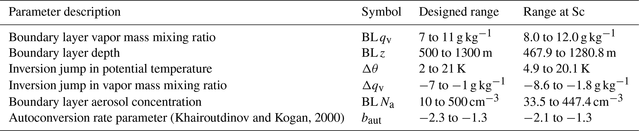
The parameter ranges were chosen to span the breadth of studies on stratocumulus-to-cumulus transitions in the subtropics. Often case studies are designed for LES simulation from observations of particularly fast or slow transitions, so a broad range of behaviours was included in the parameter space by spanning these reported cases (Sandu and Stevens, 2011; de Roode et al., 2016; Blossey et al., 2021). Although SST varies along the airmass trajectory, we chose not to include perturbations to SSTs or SST gradients among the parameters we investigated. To be useful, such a study focusing on cloud feedback would need to consider realistic covariations of SSTs with the cloud-controlling factors under investigation. Since many LES studies have not focused on the aerosol effect, the range for the accumulation mode concentrations was informed by the Cloud System Evolution in the Trades (CSET) and Marine ARM GPCI Investigation of Clouds (MAGIC) campaigns, which took place in the NE Pacific (Bretherton et al., 2019; Painemal et al., 2015). Note that we have not included extremely polluted cases, such as the biomass burning region off the western coast of Africa. There are many studies of the aerosol semi-direct effect on the stratocumulus-to-cumulus transition in the Atlantic ocean, with some contradicting results (Yamaguchi et al., 2015; Zhou et al., 2017; Diamond et al., 2022). Further understanding of transition mechanisms will help to untangle these joint effects.

2.2.1 Boundary layer vapor mass mixing ratio

The boundary layer vapor mass mixing ratio (specific humidity) directly determines at what point saturation is reached and how much moisture is available for cloud droplets to form. It also determines how much drizzle will be evaporated below cloud base.

2.2.2 Inversion properties

The strength of the inversion was perturbed by two properties: the jump in potential temperature and specific humidity across the inversion. The dissipation of the stratocumulus cloud is a defining feature of the transition and is largely caused by the entrainment of warm, dry air from above the inversion, via overshooting cumulus plumes. Thus, the rapidity of this dissipation is related to the strength of the inversion and the specific humidity in the free troposphere (Wood et al., 2018), which can be perturbed with the changes in temperature and moisture across the inversion (the jump in potential temperature will be used interchangeably with inversion strength). Additionally, the free-tropospheric humidity determines the rate of longwave cooling, which affects entrainment and evaporation (Siems et al., 1993).

2.2.3 Boundary layer depth

The boundary layer depth determines how well the layer can mix and consequently how well supplied with surface-evaporated moisture the stratocumulus cloud layer is. Eastman and Wood (2016) showed that precipitation may have opposite effects on stratocumulus cloud transitions depending on whether it is occurring in deep layers, leading to break up, or shallow layers, leading to cloud persistence.

2.2.4 Boundary layer aerosol

The initial boundary layer concentration of accumulation mode aerosol was perturbed because the vast majority of aerosols that activate into cloud droplets (cloud-condensation nuclei) are from the accumulation mode. Boundary layer Aitken mode was initialised with a concentration of 150 cm⁻³ and allowed to freely evolve. Free-tropospheric aerosol can also be a source of cloud-condensation nuclei and could be important in simulations with very low aerosol concentrations in the boundary layer (Wyant et al., 2022). However, free-tropospheric aerosol concentration was kept constant across the PPE because it was not expected to be as important as the key factors chosen. The free-tropospheric Aitken concentration was 200 cm⁻³ and the accumulation concentration was 100 cm⁻³. There is no surface source of aerosol throughout the simulations.

2.2.5 Autoconversion rate parameter

The autoconversion rate determines how readily cloud droplets form rain droplets in a parameterisation of the collision-coalescence process. In the Khairoutdinov and Kogan (2000) parameterisation, the autoconversion rate is given by

$$\begin{array}{}\text{(1)}& {\left({\displaystyle \frac{\mathit{\delta }{q}_{\mathrm{r}}}{\mathit{\delta }t}}\right)}_{\mathrm{auto}}=\mathrm{1350}{q}_{\mathrm{c}}^{\mathrm{2.47}}{N}_{\mathrm{d}}^{b_{\mathrm{aut}}},\end{array}$$

where q_r is the rain mass-mixing ratio, q_c is the cloud liquid mass-mixing ratio (both in kg kg⁻¹), N_d is the cloud droplet number concentration (cm⁻³), and b_aut is a model parameter. We perturbed b_aut from the default value of −1.79 to perturb the autoconversion rate. The default parameter values were estimated in Khairoutdinov and Kogan (2000) by reducing the mean squared error between the above function and an explicit microphysics model, and there are large uncertainties surrounding each of these values.

2.2.6 Perturbation method

The perturbation values were chosen using a “maximin” Latin hypercube approach. Figure 1 shows the 6-dimensional design, which maximizes the minimum distance between points to ensure that values are well-spaced across the multi-dimensional parameter space and unique along each parameter axis (Morris and Mitchell, 1995; Jones and Johnson, 2009). Perturbing parameters simultaneously whilst ensuring uniqueness in every dimension ensures that each simulation provides valuable new information about the model behaviour across parameter space, especially if some dimensions (parameters) do not affect the model output. Crucially, this allows sufficient sampling of parameter space with a smaller number of simulations than a grid approach. The values for the autoconversion parameter have been transformed using the inverse log because it is the exponent of N_d, i.e., the resulting autoconversion rates were approximately uniformly distributed, rather than the parameter values. The inset of Fig. 1 shows how these values in parameter space translate to initial conditions in the idealized model set up. The perturbed cloud-controlling factors evolved during model spinup and, in some simulations, before a stratocumulus cloud formed. Although the parameter space changed, the points remained spaced well enough for emulating, so we analysed the relationships between the values at the beginning of stratocumulus and the transition properties.

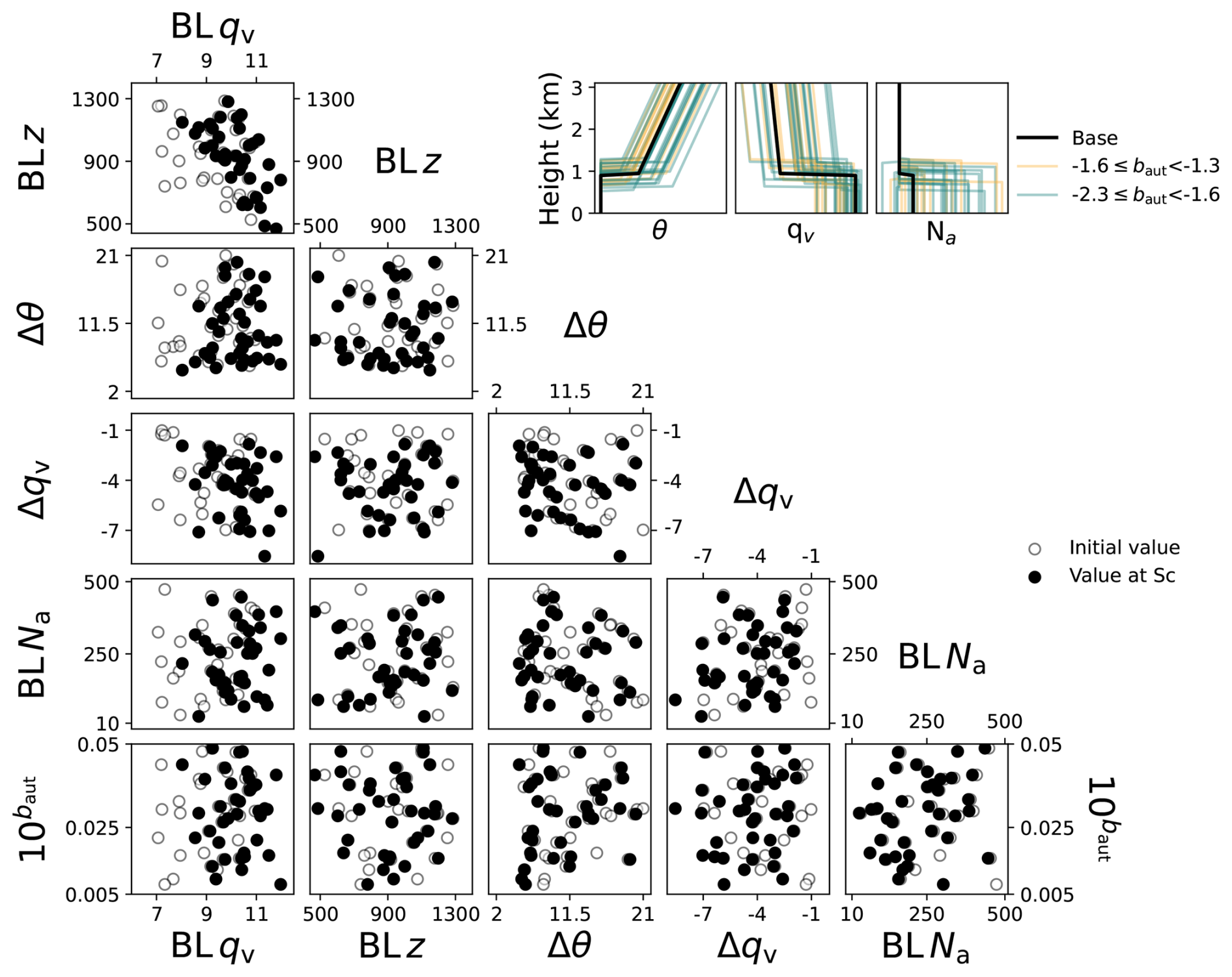
Figure 1 The Latin hypercube design for the 34-member perturbed parameter ensemble. Each 2-dimensional plot shows a different combination of two of the six parameters over the chosen ranges (see Table 1). The grey circles show the values used for the initial conditions in each simulation from the original Latin hypercube design and the black points show the evolved values at the beginning of stratocumulus for the members that developed stratocumulus and transitioned. The inset shows how the parameters are perturbed in the initial profiles using this design.

We ran 85 simulations initially, but found that 31 did not form stratocumulus because the boundary layer was too shallow and dry. Out of those simulations that had stratocumulus, 26 did not transition to a cumulus state before the end of the simulation. It is unsurprising that not all of the simulations produced transitions because the initial conditions were broadly perturbed to sample a wide range of model behavior and not all parts of the joint parameter space are expected to be realistic. The remaining 28 simulations that transitioned to cumulus were augmented by 6 transitioning simulations, out of 12 points that were augmented to the original design. These points were augmented to fill the regions of parameter space that produced stratocumulus and were likely to transition within simulation time, increasing the density of information in the most relevant part of parameter space. In total 97 simulations were run with a final 34 simulations showing cloud transitions that matched our definition of a stratocumulus-to-cumulus transition.

2.3 Transition properties

The transition properties analysed here are the transition time and the mean rain water path (R). The transition time is the time taken to transition from a stratocumulus regime (beginning at T1) to a cumulus regime (beginning at T2). Figure 2 shows two examples of how this was calculated from the cloud fraction (f_c) for all the ensemble members based on f_c>0.9 for stratocumulus and f_c<0.55 for cumulus. The value of 0.55 for cumulus was chosen as a reasonable value for a cloud transition that maximised the number of transitioning ensemble members available for emulation. The sensitivity test in Appendix A shows that the key conclusions are statistically significant down to a threshold f_c of 0.47, after which not enough simulations transition within the simulation time to give statistically significant information about the effects of different factors on the transition time. Figure 2a shows the base simulation, which has stratocumulus from the start of the simulation (T0) so T1 is set equal to T0, although realistically T1 could be earlier. The f_c decreases below the cumulus threshold just after 50 h, but it recovers until the final time step when it reaches the threshold again, T2, giving a transition time of about 68 h. It is possible the cloud could recover again if a longer simulation were conducted, which creates some noise in the calculation of transition time. Figure 2b shows a simulation that takes about 12 h to build up stratocumulus, hence subtracting T2 from T1 gives a transition time of about 32 h.

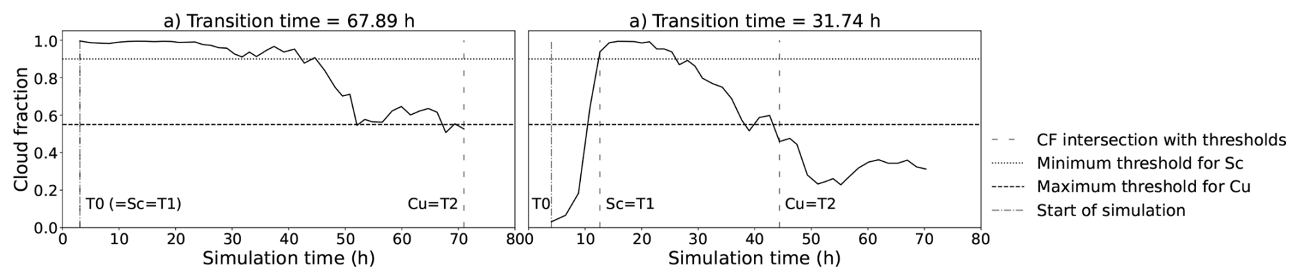
Figure 2 Transition time calculation based on cloud fraction. (a) shows an ensemble member that has stratocumulus from the start of the simulation. (b) shows a member that takes about 12 h to build stratocumulus. The solid black line is the cloud fraction timeseries, the dotted line is the 0.9 threshold which is the minimum for stratocumulus, the dashed line is the 0.55 threshold which is the maximum for cumulus. The loosely dashed lines is where the cloud fraction intersects with the stratocumulus (Sc) and cumulus (Cu) thresholds.

2.4 Gaussian process emulation

Gaussian process emulation is a Bayesian machine learning method to learn the relationship between a set of input parameters and an output of interest (Rasmussen and Williams, 2006; O'Hagan, 2006). It uses a prior specification of the relationship consisting of a mean function (e.g., constant or linear) and a covariance structure. Here we use a constant mean function for transition time, a linear mean function for mean R, and the Matérn 5/2 covariance structure. The prior is updated using a set of training data, which is the set of perturbed inputs and corresponding outputs from the PPE, to create a posterior specification. Once validated, the emulator can be used to predict values for new sets of input values, with quantified accuracy.

The emulators of transition time and mean R were validated using the leave-one-out method. Here, an emulator is created from all but one of the training points and then used to predict a value for that left-out point. This is repeated for each point in the training set and the differences between the predicted values and the actual values are used to gauge how reliably the emulator can reproduce model output. Figure 3 shows that the training points were predicted within the 95 % confidence intervals for all of the points for transition time and mean R. However, the confidence intervals are quite large, especially in the transition time where some points are up to 10 h out in the predictions. The mean R emulates slightly better, which may be because it is easier to quantify than the transition time. There is some noise in the transition time calculation due to the simulation sometimes ending before it is obvious that the cloud has fully transitioned. The noise incurred in the transition time calculation is discussed in Sect. 4. We additionally validated the emulators by calculating the ratio of the standard deviation of the mean values at the training data (a measure of variation in emulated output) to the mean of the standard deviation of those points (the uncertainty in emulated values). For both emulators, this ratio is larger than 1, which tells us the function changes more than the underlying emulator uncertainty. If the ratio was less than 1, the emulator uncertainty would be too large compared to changes in the function, so it would not be a useful approximation of the relationship. This validation shows that the emulators predict model output with sufficient accuracy for us to gain important insights into the processes that drive transitions.

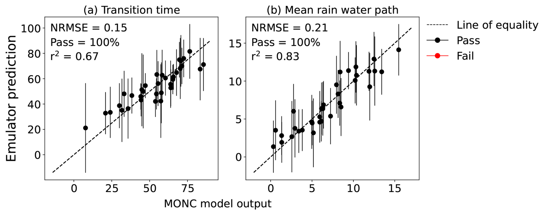
Figure 3 Emulator validation using the leave-one-out approach. (a) Transition time and (b) rain water path averaged over the transition. Both emulators were trained with the 34-member PPE. Points show the model output against the emulator-predicted values for each training data point that has been left out of the emulator training set in turn. Lines show the upper and lower 95 % confidence bounds. Black points are where the model output data lies within the confidence bounds (pass) and red points are where this is not the case (fail).

Following Sansom et al. (2024), we ran some initial condition ensembles to gauge the internal variability of the model, so that a “nugget” term could be added to the emulators. The nugget term allows the posterior mean function to have a buffer around each training point, rather than interpolating them exactly. This is useful when the data are noisy or, as in this case, for incorporating internal variability. At four training points we ran four extra simulations and varied the random seed in the model that initiates turbulence, which allowed us to calculate the approximate variance due to internal variability in the transition time and mean R. In three of these initial-condition ensembles, the members all transitioned within a few hours of each other, but in one ensemble the cloud recovered and did not fully transition until early the next day (approx. 10 h later). Adding this variance into the emulators accounts for some of the noise created in the transition time calculation (Sect. 2.3). Details of this calculation can be found in Sansom et al. (2024) and in the code repository (Sansom, 2026a).

2.5 Variance-based sensitivity analysis

We used a Python package to calculate the Sobol indices, which obtain the contributions of variance in each parameter to the variance in the outputs that we are emulating (Sobol, 2001). We discuss the “main effect”, which is how much of the variance in the output is due to the variance in the individual parameter, and the interactions which are the portion of the variance that cannot be explained by linear combinations of the individual parameters, and is attributed to the interactions between parameters.

3 Results

We begin by evaluating the cloud properties in the base simulation (Sect. 3.1), which is central to our PPE design. We then discuss the f_c timeseries across the ensemble (Sect. 3.3), before assessing the controls on transition time (Sect. 3.4) and drizzle (Sect. 3.5) using the emulators.

3.1 Cloud properties in the base simulation

The stratocumulus-to-cumulus transition in the base simulation is similar to that of previous LES studies based on the Sandu and Stevens (2011) composite case (see also, Bretherton and Blossey, 2014; Yamaguchi et al., 2017). Figure 4a–c all show a distinct diurnal cycle in f_c, liquid water path (L) and R. The f_c is defined as the fraction of cloudy columns with a cloud liquid mass-mixing ratio greater than 0.01 g kg⁻¹. The stratocumulus initially has a high f_c and is not drizzling. Through the first night the cloud begins to drizzle and through the second day the f_c and L are lower than the first day. The cloud drizzles more through the second night, further depleting L and N_a (Fig. 4d). During the third day it breaks up more into cumulus-like clouds and only recovers slightly through the night. Figure 4d shows that the domain-mean accumulation mode aerosol decreases gradually throughout the simulation and the Aitken remains fairly constant. Figure 4e–j shows three snapshots from 09:00 p.m. local time for each day of the simulation. At 09:00 p.m. local time on the first day (e–f) there is a uniform stratocumulus cloud with f_c = 0.99. The inversion height, and cloud top, are around 1000 m with a cloud layer thickness of about 300 m. At the same time on day 2 (g–h) there is a slightly more broken cloud but still a high f_c of 0.94. The cross section shows that the boundary layer deepened and cloud top rose by a couple of hundred metres during the intervening day. The lowest cloud base is around 800 m, but now the base marks the bottom of cumulus-like plumes that feed into the higher stratocumulus cloud base, around 100 m above. Since the first day, L has decreased towards the edges of the cloud and thickened towards the middle of the cell. as the stratocumulus layer thinned. At the end of the third day (i–j) there is a much more broken cloud, with f_c = 0.53, and cumulus plumes in a layer below. At this stage the boundary layer is around another 100 m deeper, and the cloud top has risen with it.

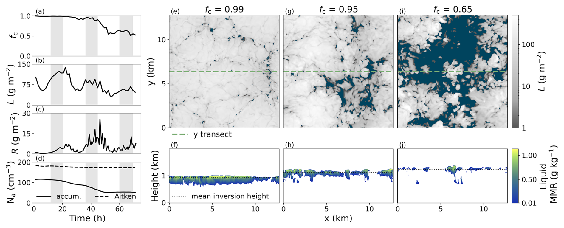
Figure 4 Base simulation cloud properties. (a–d) Timeseries of cloud fraction (f_c), liquid water path (L), rain water path (R), and boundary layer aerosol concentrations (N_a). Grey shading indicates local nighttime. (e–j) Snapshots at 09:00 p.m. local time on day 1 (e–f), day 2 (g–h) and day 3 (i–j). Top row (e, g, i) shows top-down views of L and bottom row (f, h, j) shows vertical cross sections of liquid water mass-mixing ratio (MMR) at the y-location of the transect line. The MMR is masked for values lower than 0.01 g kg⁻¹, in line with the f_c definition.

Compared to other studies that simulated this composite case, the boundary layer did not deepen to the same degree and there was less drizzle. Other LES models simulated a boundary layer depth between 1.5 to 2.5 km, whereas our simulation has a maximum depth of 1.4 km (Sandu and Stevens, 2011; Bretherton and Blossey, 2014; de Roode et al., 2016; Yamaguchi et al., 2017). This could be due to the different numerical methods, radiation schemes and mixing processes in the models, or to the stretching of the vertical layers in the top of the domain. Yamaguchi et al. (2017) is the only study using aerosol processing that we compared our base simulation to. In our simulation, Fig. 4c shows that R peaks at about 25 g m⁻² at the beginning of the third day, which aligns roughly with the sensitivity tests in Yamaguchi et al. (2017), which also used the Khairoutdinov and Kogan (2000) parameterisation in a similar domain size. However, it is much less than the peak of 150 g m⁻² for the same domain size using their bin-emulating bulk microphysics scheme. The transitions in our simulations may be slower than those in the previous studies because the shallower boundary layer may limit the boundary layer decoupling and the lower R may limit the potential for a drizzle-depletion mechanism.

3.2 PPE summary

The whole PPE is summarised in Fig. 5 by splitting it into three categories: members that did not transition, members that transitioned with low mean R, and members that transitioned with high mean R. The simulations with high mean R generally started with a higher temperature inversion, i.e., a deeper boundary layer, and on average the boundary layer deepened less throughout the simulation than those that had lower mean R or did not transition. The lifting condensation level lowers throughout the simulations for all members, but slightly more for the high mean R set. The decoupling factor was calculated as the relative decoupling index from Kazil et al. (2017), $\frac{z_{\mathrm{CB}}-z_{\mathrm{LCL}}}{z_{\mathrm{LCL}}}$, which is based on Jones et al. (2011), where z_CB is the cloud base and z_LCL is the lifting condensation level. Cloud base was calculated as the domain-mean cloud base where cloud is present in the column. The high mean R set also decouples faster than the other sets, with the non-transitioning set being slowest to decouple. The high mean R set has significantly more surface precipitation than the other sets, with the non-transitioning set having the least. The non-transitioning set maintains a high f_c until the very end of the simulation time, while the transitioning sets show f_c decreasing significantly from day 2 (high mean R) and day 3 (low mean R). There is not much distinction in L between the sets, except the non-transitioning set increases more during the second night. The high mean R set has a much higher mean R in the first night and second day, but the other sets increase steadily from the second night onward. On average, the low mean R set has a lower median initial BL N_a than the other sets, but the median BL N_a decreases at the same rate as the non-transitioning set. The high mean R shows a faster initial decrease through the first night and second day, when it has the highest R.

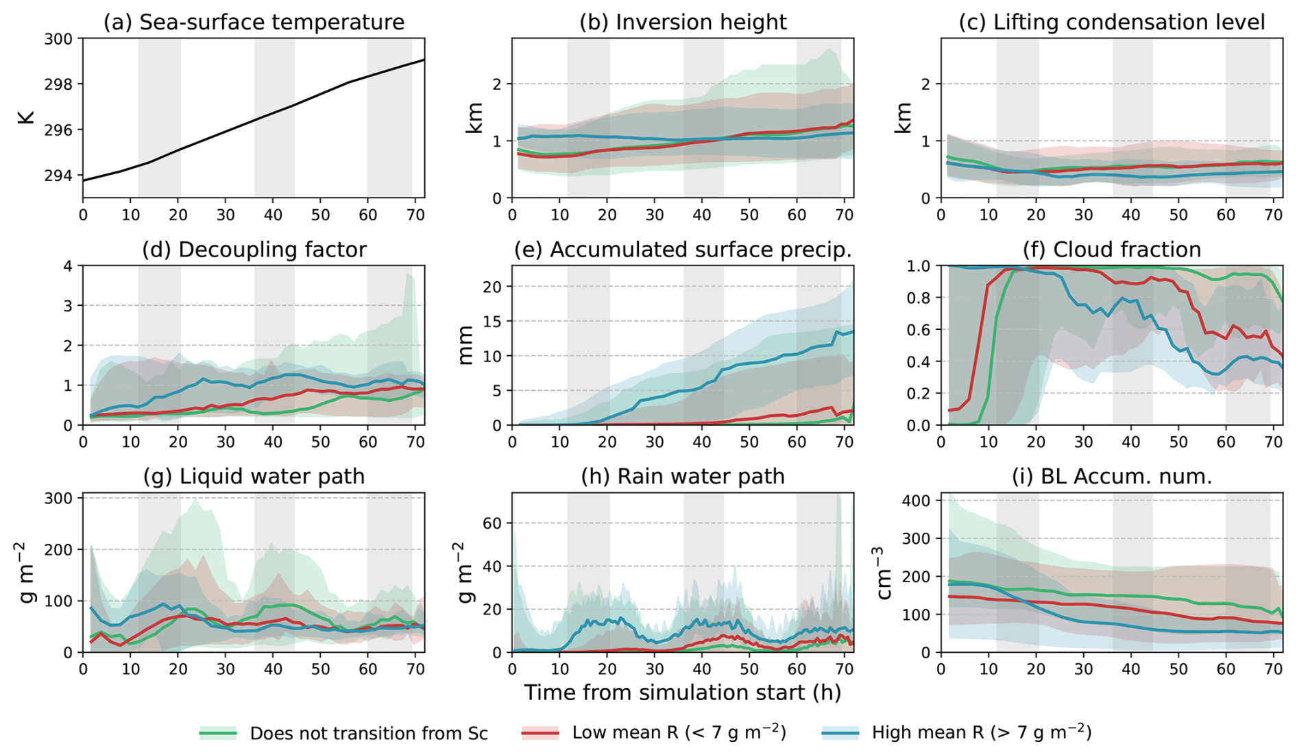
Figure 5 Summary of the whole PPE. (a) Sea-surface temperature forcings applied to all simulations, (b) temperature inversion height, (c) lifting condensation level, (d) decoupling factor, (e) accumulated surface precipitation, (f) cloud fraction, (g) liquid water path, (h) rain water path, and (i) boundary layer accumulation mode number concentration. The PPE is split into three categories (1) members that formed stratocumulus but did not transition, (2) members that transitioned but had a mean rain water path of less than 7 g m⁻², and (3) members that transitioned but had a mean rain water path of more than 7 g m⁻². The line shows the median of each subset and the shading shows the minimum and maximum of the subset. The grey shading indicates local nighttime.

3.3 PPE cloud fraction analysis

Figure 6a shows that the range of initial f_c produced across the PPE is large, as expected from perturbing many initial conditions over a large range of environmental conditions. Those that form stratocumulus (67 simulations, Fig. 6b) and those that form cumulus (37 simulations, Fig. 6c) make up the ensemble subset that transition. The subset mean in Fig. 6c has a similar shape to the base simulation, but the subset mean transitions a few hours earlier. However, the PPE members show a wide range of behaviours. On average, f_c stays near one through the first day and night, before dipping in the second day to f_c ≈ 0.75 and on the third day it crosses the cumulus threshold and stays below. A diurnal cycle can be seen in many of the members, with some members dipping to f_c ≈ 0.4 and still recovering in the second night. Additionally, some members keep f_c ≈ 1 until the third day and then transition rapidly.

Figure 6 Cloud fraction timeseries for (a) the whole ensemble, (b) the members that form stratocumulus, (c) the members that also form cumulus, and (d) as in (c) but aligned to the start of stratocumulus, T1. The thick, solid, black lines show the mean of the timeseries. The vertical lines show the start time of stratocumulus for each member, coloured either green or yellow depending on whether the SST at the start of stratocumulus is below or above 296 K. The ensemble members in (d) are coloured by the SST threshold as well. The solid, green line shows the mean of the ensemble without the high SST members.

While many of the simulations that transitioned formed stratocumulus within the first day, there were three simulations that only formed stratocumulus beyond the end of the second day when the SST had increased by at least 1 K and these transitioned very quickly. The transitioning simulations are “epoch aligned” in Fig. 6d by aligning T1 for each member, and the high SST members are highlighted. These fast transitions occur despite being in areas of parameter space where you might not expect it, for example in a very shallow boundary layer with a low autoconversion rate. This subset of simulations shows that warmer initial SSTs may act to considerably speed up the transition, above meteorological conditions, which has implications for the future warmer climate. However, the PPE does not have enough simulations with warm SST to draw a definitive conclusion. The warm SST simulations have been removed from this analysis (leaving 34 simulations) since the difference in SST at initial stratocumulus is akin to perturbing a seventh parameter, but one that was not initially accounted for in our experimental design.

3.4 Transition time analysis

3.4.1 Space-filling predictions

The emulator's posterior mean response surface was used to make 1000 predictions of transition time, which fill the parameter space and provide far more information than the raw PPE data alone. These 1000 points are sampled from the emulator’s posterior mean distribution using a Latin hypercube design, so each point varies in all 6 dimensions. Figure 7 immediately begins to inform us about the subtleties in variation across parameter space. Some of the 2-dimensional subplots show clear variations, which means the transition time varies consistently for those two parameters over all values of the other parameters that are not shown in that panel (e.g., Fig. 7k and o). Other subplots show less clear variations of the transition time for the two parameters, which suggests there is no obvious dependence on these two parameters, or the effects of the four hidden parameters are dominating (e.g., Fig. 7a and c). There is a strong variation in transition time over the boundary layer aerosol concentration range, BL N_a, with low BL N_a producing the fastest transitions (Fig. 7d, h, k, m, o). The inversion strength Δθ in Fig. 7b, f, j, k, l and the autoconversion parameter (${\mathrm{10}}^{b_{\mathrm{aut}}}$ along the bottom row) also cause strong variations in the transition time, which are particularly clear in combination with BL N_a (Fig. 7k and o).

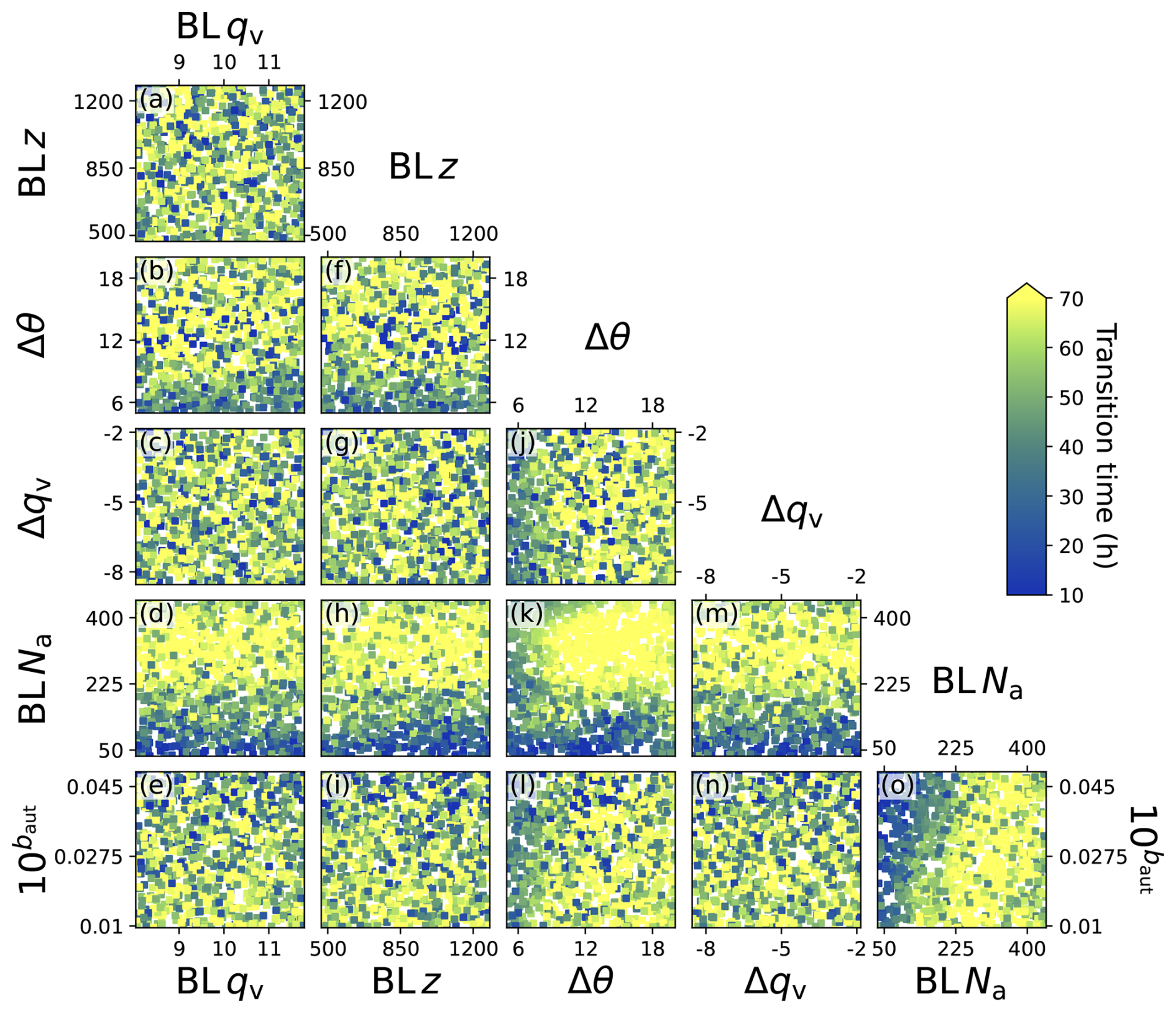
Figure 7 Transition time emulator sampled with a 1000-point Latin hypercube. (a)–(o) shows each 2-dimensional combination of the six factors perturbed in the ensemble across the chosen ranges.

3.4.2 Transition time average response surfaces

The strength of the output's dependency on each parameter and the joint effects of parameters can be more easily interpreted using an averaged response surface. Figure 8 shows 1 million grid-based points sampled from the emulator’s posterior mean distribution and averaged through the 4 dimensions not shown in each 2-dimensional panel. The transition time has the strongest dependencies on aerosol concentration (BL N_a), inversion strength (Δθ), and the autoconversion parameter (b_aut). Many panels show linear individual effects (e.g., Fig. 8g and j) but several show non-linear joint effects (or interactions, shown by curved surfaces e.g., Fig. 8f, k, o) between parameters. Here we discuss the dependencies visualised in the response surfaces in Fig. 8 and suggest mechanisms from relevant studies.

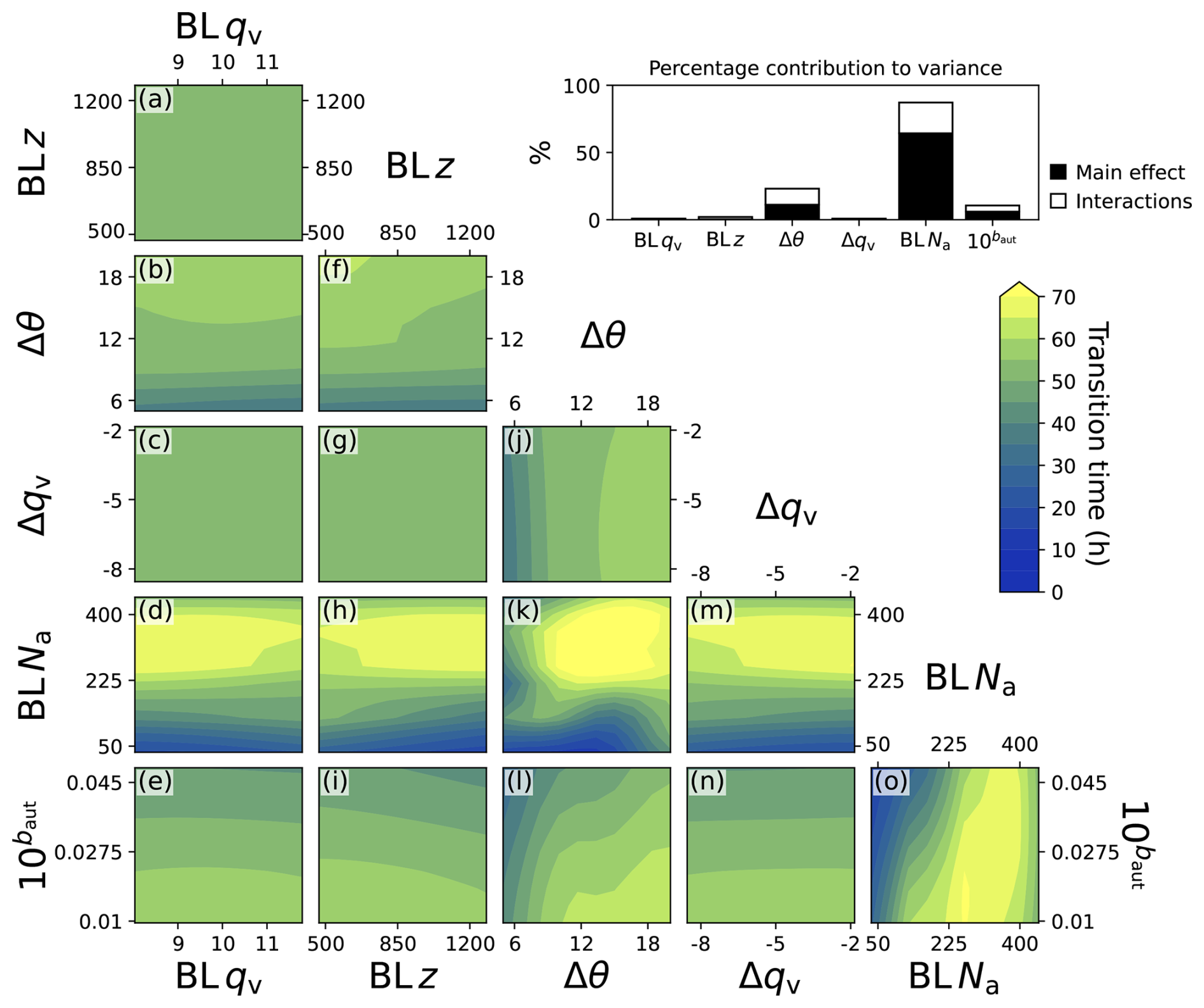
Figure 8 Averaged transition time response surface. The transition time emulator was sampled 1-million times using a 6-dimensional grid and (a)–(o) shows each 2-dimensional combination of the six perturbed factors averaged through the remaining 4 dimensions not shown in that panel. The inset in the top right shows the contribution of each parameter's variance to the variance in the transition time.

The transition time has the strongest dependency on aerosol concentration, BL N_a, (see Fig. 8d, h, k, m, o) with the fastest transitions corresponding strongly to stratocumulus in environments with low aerosol concentrations. The transition time is only predicted, on average, to be below 40 h for BL N_a below 200 cm⁻³. There are clear joint effects with BL z, Δθ, Δq_v and b_aut (Fig. 8h, k, m, o). Yamaguchi et al. (2017) and Diamond et al. (2022) found that low aerosol environments caused drizzle depletion of moisture and aerosol in the boundary layer. The deeper analysis in Yamaguchi et al. (2017) found that in their simulations it was specifically cumulus drizzle being lifted to the stratocumulus layer and initiating a rapid depletion. Erfani et al. (2022) found that adding aerosol into a clean case caused a delay in the transition, but adding aerosol into a polluted case had little effect on the transition time.

The next strongest dependency is on the inversion strength, Δθ (Fig. 8b, f, j, k, l). The fastest transitions occur for stratocumulus under weak inversions (small Δθ) and the slowest transitions occur under strong inversions (large Δθ). There are clear joint effects with BL z, BL N_a and b_aut (Fig. 8f, k, l). Several studies have found the inversion strength, or the closely related lower tropospheric stability, to be a key control on the transition time (Mauger and Norris, 2010; Sandu and Stevens, 2011; Eastman and Wood, 2016). These studies showed that clouds under weak inversions are prone to break up or that clouds under strong inversions persist. Strong inversions can trap moisture in the boundary layer and reduce boundary layer deepening and decoupling, which is a key stage in the classic transition.

The third strongest dependency is on the autoconversion parameter, shown here as 10${}^{b_{\mathrm{aut}}}$ to be uniformly spaced (Fig. 8e, i, l, n, o). The fastest transitions occur for high autoconversion rates. There are joint effects with BL z, Δθ and BL N_a (Fig. 8i, l and o). Higher autoconversion rates would induce a drizzle-depletion effect as already discussed. In addition to the previously mentioned studies, Eastman and Wood (2016) found a small, non-linear effect where precipitation sustains cloud cover in shallow boundary layers but promotes cloud breakup in deep boundary layers.

The transition time has very weak dependencies on the remaining parameters. The boundary layer depth, BL z, shows that stratocumulus in deep boundary layers transition faster on average than in shallow boundary layer (Fig. 8a, f, g, h, i). The slight dependency of transition time on BL z is seen more clearly in the joint effects with Δθ, BL N_a and b_aut (Fig. 8f, h, i). Wood and Bretherton (2006) showed that deep boundary layers are more likely to be decoupled and, since decoupling is part of the classic transition mechanism, this stage could be accelerated when beginning in a deeper boundary layer. Eastman and Wood (2016) found that clouds in deep boundary layers are prone to break up, and they also suggested the transition occurs through decoupling. The transition time is nearly invariant to changes in the jump in specific humidity, Δq_v (Fig. 8c, g, j, m, n), and to changes in boundary layer specific humidity, BL q_v, for any conditions of the other parameters (Fig. 8a–e).

The transition time sensitivity analysis (top right of Fig. 8) quantifies the effects described above in terms of the main effects (the average effect of a factor across all values of the other factors) and interactions. On average, the BL N_a main effect has the largest contribution to the variance in the transition time of 64 %. The average Δθ main effect contributes 11 %, b_aut contributes 6 %. The remaining parameters contribute less than 1 % each. The interactions from each parameter contribute a total of around 18 % of the variance, so the total interactions are more important than some of the parameter main effects. The dependence on the interactions between parameters demonstrates the complexity of the transition time drivers that more traditional studies have not managed to capture.

3.5 Mean rain water path (R) analysis

We analysed mean R to determine whether the drivers of the transition might have acted through a drizzle-depletion mechanism. The PPE mean R is summarised in Fig. 9, with the domain-averaged timeseries for each member shown in Fig. 9a. The PPE is split into “low” (red) and “high” (blue) R by a temporal mean threshold of 7 g m⁻² (approximately half of the highest member). The BL N_a (panel 9b) and the f_c for the transitioning simulations (aligned by T0s in Fig. 9c and epoch aligned by T1s in Fig. 9d) have also been coloured low and high for R with corresponding subset means. The histograms in Fig. 9e and f show the number of points being averaged over at a given time in each subset, which varies because of the different stratocumulus formation times (Sect. 3.3 and Fig. 6).

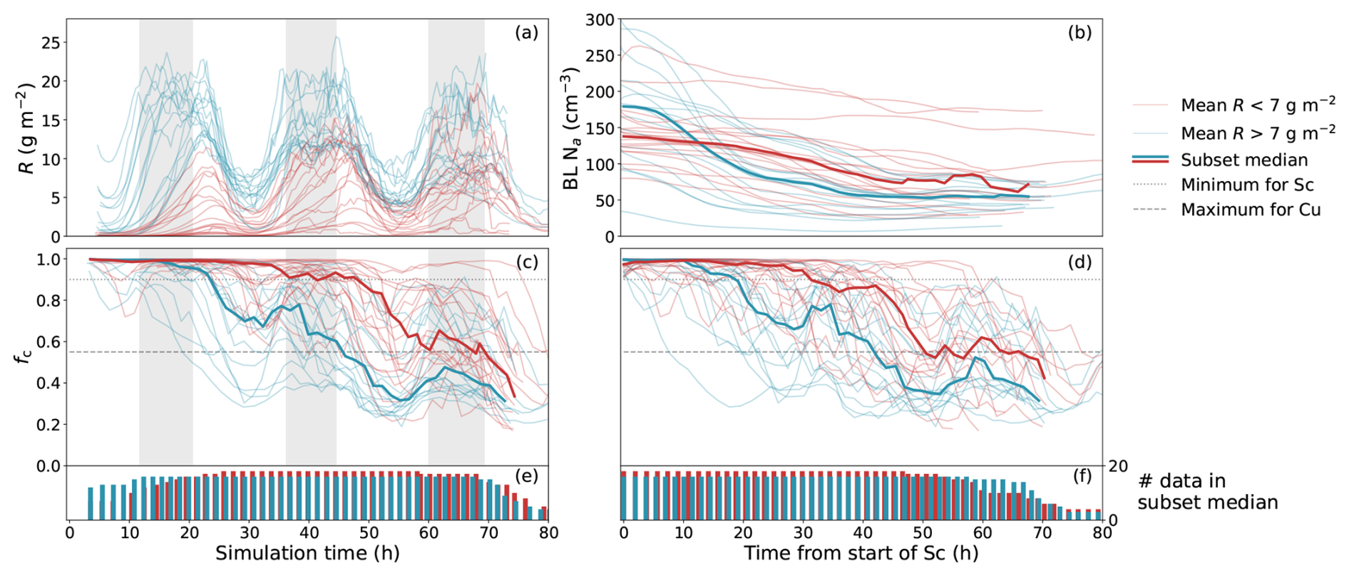
Figure 9 Ensemble timeseries split by mean rain water path. (a) The domain-averaged rain water path timeseries for each member split by temporal mean rain water path greater than 7 g m⁻² (blue) or less than (red). (b) The boundary layer accumulation mode aerosol aligned to T1 and coloured by mean R. (c) The cloud fraction timeseries as in Fig. 6c but coloured by mean R. (d) As in (c) but aligned to T1. The means over each subset (high or low mean R) are shown in bold. (e) The number of data points used in calculating the mean of each subset at each timestep in (c). (f) As in (c) but for (b) and (d).

We find that the set of simulations with higher mean R transitioned approximately 24 h ahead of those with lower mean R (Fig. 9d). Figure 9a shows that those with higher mean R mostly produced drizzle in the first two days, whereas for those with lower mean R the drizzle gradually builds through the simulation. Figure 9b shows that in most simulations the BL N_a decreases. It also shows that the higher mean R subset has a median concentration that is initially higher than the lower mean R subset, but it decreases more sharply over the first 20 or so hours from T1. After 20 h, the gradient of the higher mean R subset levels out to be similar to the lower mean R subset. In Fig. 9c, the timeseries are lined up with the diurnal cycle and it shows that the high R subset mean recovers more than the low R mean during the nights. This could be similar to the behaviour shown in Sandu et al. (2008), where the drizzling stratocumulus case recovers to higher L values through the night compared with the suppressed precipitation case, which is driven more by entrainment than longwave cooling. However, Fig. 9c shows that some of the high R cases follow a more extreme diurnal cycle than the low R cases.

Figure 10 shows that by splitting the ensemble into the high and low mean R subsets, some of the marginal correlations become stronger. Figure 10a shows Δθ has a stronger correlation with transition time when only considering the low mean R cases, and the correlation is otherwise insignificant. Conversely, BL N_a has a stronger correlation with transition time when only considering the high mean R cases. Figure 10c shows that although the fastest transitions do have a higher mean R, drizzle is clearly not the only important factor determining the transition time. Rather, other factors affect the characteristics of the transition, such as the degree of decoupling and the ability to recover through the night. It should be noted that with the inclusion of the high SST ensemble members, any correlation of mean R with transition time vanishes. This suggests that this correlation may not be significant if a wider array of deepening-decoupling mechanisms were represented.

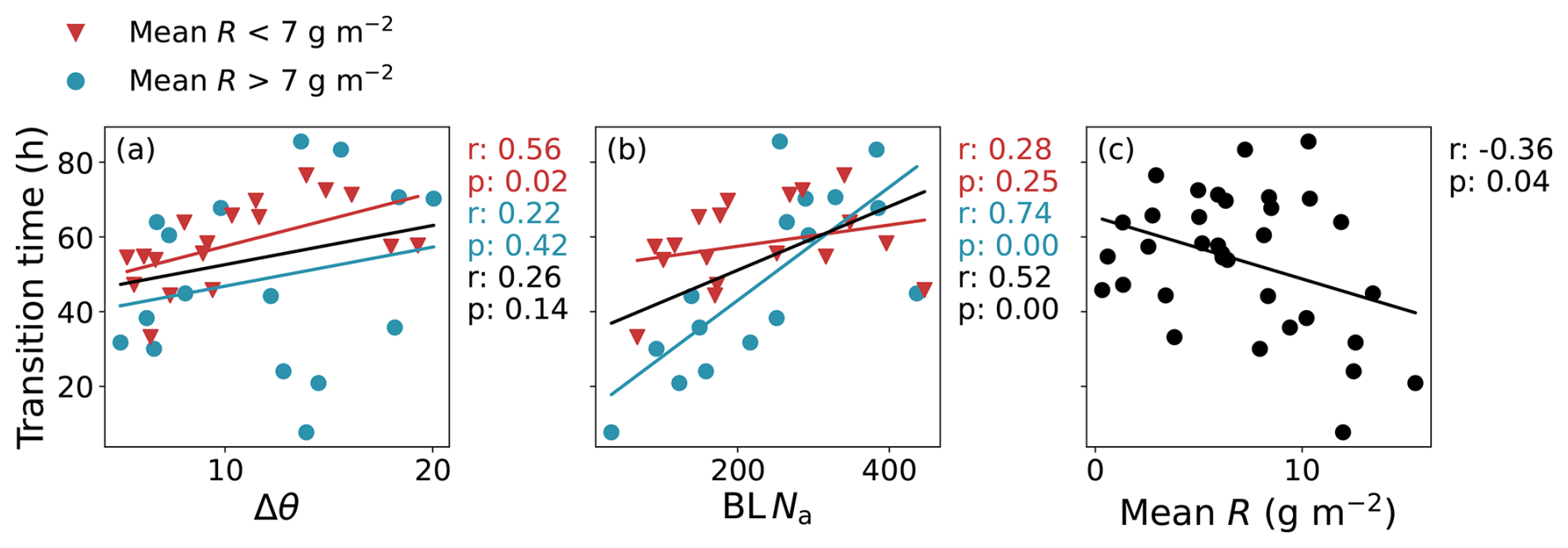
Figure 10 One-dimensional scatter plots of (a) Δθ, (b) BL N_a and (c) mean R against transition time for a cumulus cloud threshold of 0.55. The scatter points show the 34 simulations that transitioned within the simulation time and are coloured by high mean R (blue circles) or low mean R (red triangles). Lines of best fit, Pearson's correlation coefficients (r) and statistical significance (p) are calculated for the whole set (black) and each subset.

3.5.1 Rainwater path average response surfaces

The average response surfaces for the mean R emulator are shown in Fig. 11. The linear contours make it immediately clear that there are fewer interaction effects compared with the transition time. The mean R has the strongest dependency on BL z, with high Rs in deep layers (Fig. 11a, f, g, h, i), which has been found in many previous studies (Bretherton et al., 2010; Eastman and Wood, 2016; O et al., 2018). The next strongest dependency is on BL N_a, with high aerosol producing less rain through precipitation suppression (Albrecht, 1989) (Fig. 11d, h, k, m, o). Additionally, there is a strong dependency on b_aut as it is directly linked to the amount of precipitation formed (Fig. 11e, i, l, n, o). For both specific humidity parameters, there is higher R for higher humidity since vapour is available for condensation (BL q_v: Fig. 11a–e and Δq_v: Fig. 11c, g, j, m, n). Finally, Δθ shows slightly higher mean R under weaker inversions (Fig. 11b, f, j, k, l), possibly because weaker inversions are more likely to rise and create deeper boundary layers, which generally drizzle more, but this is a very weak relationship.

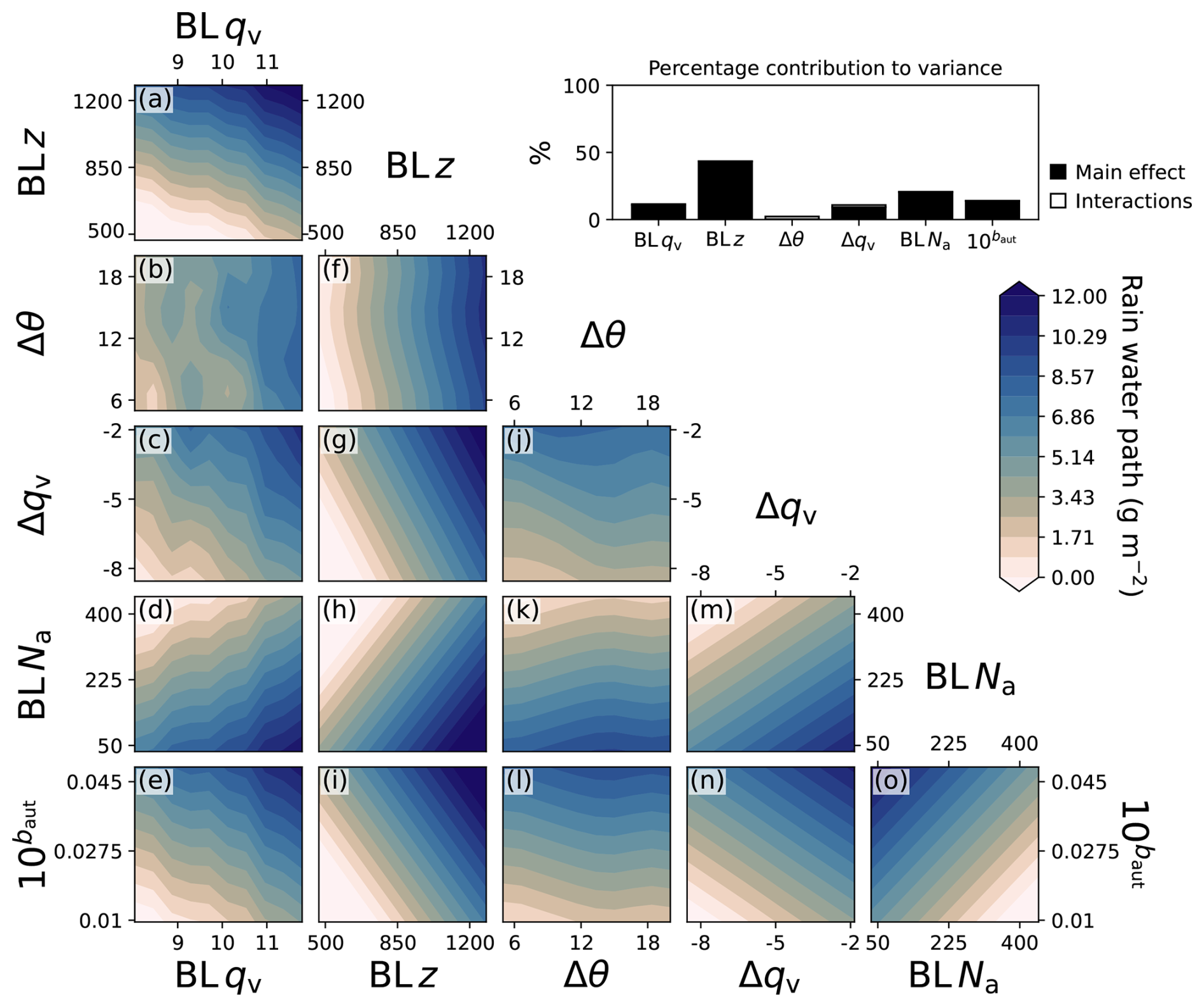
Figure 11 Average rain water path response surface sampled with a 1-million point 6-dimensional grid and averaged across hidden dimensions. (a)–(o) shows each 2-dimensional combination of the six perturbed factors averaged in the four dimensions not shown. The inset in the top right shows the contribution of each parameter's variance to the variance in the rain water path.

The sensitivity analysis of the mean R emulator, shown in top right of Fig. 11, quantifies the effects described above and shows the variance is widely influenced by all parameters rather than being dominated by one specific parameter, like transition time. The BL z contributes most to the variance in R (43 % on average). This is followed by BL N_a (20 %), b_aut (14 %) and both specific humidity parameters at about 10 %. The Δθ contributes less than 1 %. The interaction effects are of little importance (2 %) in comparison to the three most important parameters. This shows that the mean R is determined more directly by single factors, rather than interactions between them.

4 Discussion and Conclusions

In this study, we have used an LES cloud microphysics model with aerosol processing to create an idealised perturbed parameter ensemble and explore the effects of aerosol and drizzle on the stratocumulus-to-cumulus transition. The ensemble is based on the Sandu and Stevens (2011) composite case, which was created to represent a typical trajectory in the NE Pacific during summer. This novel approach offers a means to investigate the mechanisms underlying the transition and is crucial for assessing the interplay of multiple contributing factors. It should be noted that highly polluted aerosol conditions and the effect of the semi-direct aerosols in plumes is beyond the scope of this study.

We find that aerosol concentration most strongly controls the transition time out of the factors considered here. In low aerosol environments with less than about 200 cm⁻³ the transition time is typically less than 40 h. These rapid transitions occur in combination with deep boundary layers or weak inversions, and are more common when using a high autoconversion rate. Boundary layer depth and aerosol concentration most strongly control the mean R, followed by the autoconversion rate. Across the full parameter space that we sampled, simulations that have a high mean R transition on average around 24 h faster than those with a low mean R. However, the importance of drizzle varies across the parameter space. The effect of drizzle is particularly strong in the low-aerosol regime, which is consistent with the drizzle-depletion mechanism. However, in the high-aerosol regime drizzle has a negligible effect and the inversion strength becomes much more important through its determination of entrainment rate and the effect on deepening-warming decoupling.

The PPE approach, with only 34 simulations, effectively captures the joint effects of several cloud-controlling factors in a multi-dimensional parameter space. Where previous studies have focused on the individual effects of parameters, we have identified key combinations of parameters that control the transition time and mean R. The PPE approach also reveals that the part of parameter space with a particularly strong aerosol effect is small, which could explain why fast transitions by drizzle depletion in the real world have not been observed. It is unlikely that campaigns, particularly in the NE Pacific Ocean off the coast of North America, will observe conditions of particularly deep, pristine boundary layers, hence there are no clear observations of a low-aerosol induced rain-hastened mechanism in this region. However, “ultra-clean layers” where the concentration of particles larger than 0.1 µm is below 10 cm⁻³, are a common feature of the transition and may be the result of the drizzle-depletion mechanism (Wood et al., 2018; O et al., 2018). We have also only considered 6 dimensions out of a much larger multi-dimensional problem. With the inclusion of other variables that could have a larger influence on the deepening-warming mechanism (such as initial SST, subsidence or wind speeds) the region with a strong aerosol effect is likely smaller than what we have shown here.

The PPE approach exposes other joint effects that were not apparent in previous studies. We find that the inversion strength has a negligible effect on the transition time in simulations with high mean R, whereas in simulations with low mean R it is the second strongest effect (slightly lower than boundary layer moisture, not shown). Previous studies have found that lower tropospheric stability, which is closely linked to inversion strength since it is the difference in potential temperature at 700 hPa and the surface, strongly controls the timing of the transition (Sandu and Stevens, 2011). Our results suggest that this is true when drizzle is playing a minor role in the deepening-warming-decoupling mechanism, but when drizzle depletion is driving the transition, the inversion strength (and consequently the lower tropospheric stability) has a weaker effect.

Uncertainty in the autoconversion parameter strongly affects the transition time and mean R. It is one of the three most important parameters for both. When uncertainty in parameterisations such as this have such a large influence on cloud bulk properties, modelling studies can produce very different results depending on where in parameter space the model lies. An example from Fig. 8 is that low autoconversion rates lower the aerosol concentration at which the transition time becomes insensitive to aerosol (and so probably more sensitive to inversion strength). The sensitivity of a model to a parameter will be affected by structural differences between models. The effects of structural differences on these sensitivities could be evaluated if other modelling groups were to replicate this work, creating a multi-model PPE.

The details of our results differ from Yamaguchi et al. (2017), but the results support the same conclusions. The drizzle-depletion effect is weaker in our simulations, which is likely due to our model producing less drizzle (seen in the base case in Sect. 3.1) and also because many of our simulations form drizzle much earlier, with peaks in the first or second day. This can still cause a drizzle-depletion effect by removing aerosol and moisture from the cloud layer, but it is unlikely to be cumulus-initiated rain causing a positive-depletion feedback because the cumulus generally formed after the second day. The causes of these differences in R are most likely due to differences in domain size or the microphysics scheme. The R values in our simulations are much closer to the values from a sensitivity test in Yamaguchi et al. (2017), which aligns better with our setup, with a domain size of 12 by 12 km² rather than 24 by 24 km² and with the Khairoutdinov and Kogan (2000) microphysics scheme rather than the bin-emulating bulk scheme (Fig. 9 and their Fig. 10c). Our study included autoconversion and supports the conclusion of Yamaguchi et al. (2017) that the lack of rain feedbacks, on aerosol and cloud droplet concentrations, in previous studies may partially explain why drizzle was found to have only a minor effect (Sandu and Stevens, 2011; Blossey et al., 2021), and the transition time to be dominated by lower tropospheric stability and entrainment rate.

Compared with other studies that simulated the composite case from Sandu and Stevens (2011), the boundary layer deepening is weaker in our simulations, and this could restrict circulation and precipitation. The maximum height of the boundary layer in our base simulation is around 1400 m, whereas other studies have deepening up to around 2500 m (Sandu and Stevens, 2011; Bretherton and Blossey, 2014; de Roode et al., 2016; Yamaguchi et al., 2017). The previous version of the MONC model was used in the de Roode et al. (2016) model intercomparison, and it has the shallowest boundary layer with a maximum height of about 1800 m for the reference case (our base case), which suggests that it could be a feature of the MONC model. A shallower boundary layer throughout the ensemble will likely delay the transition time in all simulations.

Unlike previous studies of the aerosol effect on the stratocumulus-to-cumulus transition, we also included Aitken and coarse mode aerosol. Merikanto et al. (2009) first showed that a significant portion of marine boundary layer cloud-condensation nuclei are formed in the free troposphere. More recently, the Aitken buffering hypothesis of McCoy et al. (2021) has been supported by simulations in Wyant et al. (2022) and McCoy et al. (2024), which show Aitken-sized aerosol can be transported to the boundary layer where the larger particles act as cloud condensation nuclei. High concentrations of Aitken mode in the free troposphere slowed the stratocumulus transition to shallow open cells, which otherwise would have occurred through aerosol removal and precipitation feedbacks. In our simulations, Aitken mode particles are not significantly depleted during the simulations, but this could be a small factor to consider. Additionally, we have not included a source of aerosol through the simulation whereas in reality, sea spray is a primary source of aerosol away from coastal environments. This source would have acted to slow all transitions equally since we did not perturb controlling factors, such as wind speed.

One challenge we faced was how to define a reliable measure of the transition time. This is less of a problem in a small set of simulations that are individually analysed, but it becomes more of an issue when building an emulator that describes the transition time across a multi-dimensional parameter space. As mentioned previously, some of the cumulus clouds may have recovered to stratocumulus after the simulation ended, as part of the diurnal cycle. Similarly for the clouds that began with stratocumulus, there is an unquantifiable amount of time before the simulation where the cloud may have been formed. It may help to spin up a base cloud before making perturbations and to have a restriction on how long the cloud must remain as cumulus before the end of the simulation. However, perturbations after spinup could cause erratic model responses, and there would still be an adjustment period that would vary across parameter space. Two alternative methods could be to study the time taken for the cloud to transition from the end point of stratocumulus to the start of cumulus, or the gradients in the decline from stratocumulus. Using f_c is a reliable way to measure a transition in cloud behaviour, but it is difficult to distinguish between an end state of mesoscale cumulus organisation and open-cell stratocumulus, especially in a domain of this size. Diamond et al. (2022) found open-cell stratocumulus in their study of the transition that used a domain of a similar size, but they did not determine under which conditions the stratocumulus transitioned to a cumulus state or an open-cell state. Despite the small domain size, further analysis of the simulations in this ensemble could give insight into this problem.

The PPE and emulator approach has allowed us to identify joint effects in the stratocumulus-to-cumulus transition, which create different regimes that align with different mechanisms. The response surfaces also visually showed that the combination of parameters required for the drizzle-depletion mechanism are not typical in the observed regions. In cloud transition studies, being able to understand the occurrence of different regimes under specific parameter combinations is a valuable tool.

Appendix A: Cumulus threshold sensitivity test

Figure A1 shows a repetition of the 1-dimensional parameter analysis from Fig. 10 to determine whether the key correlations still hold for a lower cumulus threshold. Here, the threshold for cumulus cloud has been reduced to a f_c of 0.47. Reducing this threshold results in a mean ensemble transition time of 57 h, which is 3 h longer than for a cumulus threshold of 0.55. The significant correlations in Fig. 10 are still significant with the lower threshold. The correlation of transition time with Δθ is slightly stronger and the correlation of transition time with BL N_a is slightly weaker.

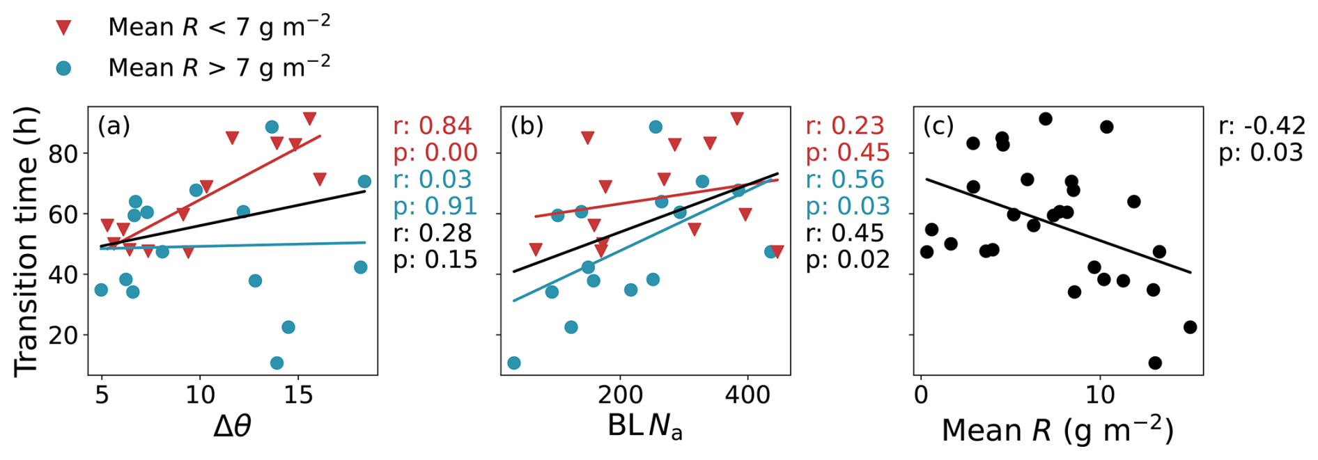
Figure A1 One-dimensional scatter plots of Δθ (left) and BL N_a (right) against transition time for a cumulus cloud threshold of 0.47. The scatter points show the 34 simulations that transitioned within the simulation time and are coloured by high mean R (blue circles) or low mean R (red triangles). Lines of best fit, Pearson's correlation coefficients (r) and statistical significance (p) are calculated for the whole set (black) and each subset.