
the Creative Commons Attribution 4.0 License.
the Creative Commons Attribution 4.0 License.
 | 19 Nov 2026
A potential emergent constraint on cloud liquid water path adjustments to aerosol–cloud interactions
Johannes Mülmenstädt

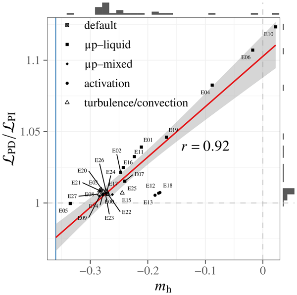
Emergent constraints are relationships between an observable in the present-day climate (such as cloud state variables) and an unobservable response (such as adjustments to radiative forcing) of the climate system to a perturbation. Here we present a candidate emergent constraint arising from the relationship across members of a perturbed parameter ensemble (PPE) between the observable present-day cloud droplet number–liquid water path (Nd–ℒ) correlation and the unobservable liquid water path adjustment to anthropogenic aerosol–cloud forcing (RAℒ). Emergent constraint candidates require scrutiny to distinguish them from, for example, spurious correlations. The candidate presented here meets several criteria delineated by Klein and Hall (2015): high correlation coefficient, plausible underlying physical mechanism, and emergence from a PPE that perturbs the physical parameters relevant to both the observable and the climate response. Constraining the observable Nd–ℒ regression slope to present-day satellite estimates yields a constrained estimate for the ratio of ℒ under present-day and preindustrial aerosol emissions (PPE regression slope uncertainty only) with a regression coefficient of 0.92. The constrained implies a robustly positive RAℒ; this disagrees in sign with all other general circulation model (GCM) estimates but agrees with non-GCM lines of evidence. However, the constrained estimate requires extrapolating the emergent constraint relationship past the minimum produced by any of the PPE members.
- Article
(1181 KB) - Full-text XML
-
Supplement
(487 KB) - BibTeX
- EndNote


Anthropogenic increases in aerosol concentration modify cloud properties in several ways that exert an effective radiative forcing (ERF) on the climate (e.g., Bellouin et al., 2020; Forster et al., 2021). The ERF can be decomposed into two components: a radiative forcing resulting from an increase in cloud droplet number concentration (Nd), and radiative adjustments resulting from changes in cloud liquid water path (ℒ) and cloud fraction as cloud processes respond to the perturbed Nd (e.g., Boucher et al., 2014; Sherwood et al., 2015; Quaas et al., 2024).
Estimates of the magnitude of the ERF from different lines of evidence traditionally disagree with one another (Boucher et al., 2014), but they have come into closer agreement (Forster et al., 2021). However, different lines of evidence still do not agree on the sign of the radiative adjustment due to ℒ change (RAℒ). Observational studies and process modeling estimates of RAℒ are slightly to moderately positive (i.e., anthropogenic aerosols lead to a reduction in ℒ and thus increase absorbed shortwave energy; Bellouin et al., 2020; Forster et al., 2021). Atmospheric general circulation models (GCMs), on the other hand, estimate RAℒ to be slightly to moderately negative (Mülmenstädt et al., 2019; Gryspeerdt et al., 2020; Smith et al., 2020).
Either sign of RAℒ is physically allowed, as the net RAℒ is the sum of two opposing-sign mechanisms: precipitation suppression (Albrecht, 1989) and enhanced evaporation (Ackerman et al., 2004; Bretherton et al., 2007). In multimodel ensembles (MMEs) and perturbed parameter ensembles (PPEs), it appears that the highest (i.e., least negative) RAℒ achievable in GCMs is within internal variability of zero. One plausible hypothesis that would explain the absence of robustly nonnegative RAℒ PPE or MME members is structural: that the process scales of entrainment, and therefore entrainment enhancement, simply cannot be represented at GCM scales without a parameterization. However, even models that parameterize or otherwise respond to increased Nd with increased cloud-top entrainment drying still produce higher mean ℒ in response to anthropogenic aerosols (Guo et al., 2011, 2014; Karset et al., 2020; Mülmenstädt et al., 2024a, b).
As the models appear structurally capable of representing both RAℒ mechanisms, a natural question to ask is whether it is possible to bring the models into agreement with other lines of evidence through parametric changes that increase or reduce the strength of each of the opposite-sign mechanisms. Furthermore, if the emergent behaviors of the model (like ERF and RAℒ) vary smoothly with changes in the model physics parameters, it may be possible to derive an emergent constraint (Klein and Hall, 2015) from PPEs. Emergent constraints are relationships between an observable in the present-day climate (such as cloud state variables) and an unobservable response (such as adjustments to radiative forcing) of the climate system to a perturbation.
Below, we document a potential emergent constraint that uses the present-day correlation between Nd and ℒ as an observable to constrain RAℒ. Intriguingly, the sign of the constrained RAℒ agrees with the Bellouin et al. (2020) multiline assessment, even though the RAℒ in every one of the underlying PPE members has the opposite sign.
2.1 Model description and physics perturbations
The U.S. Department of Energy's Energy Exascale Earth System Model (E3SM) (Golaz et al., 2019) Atmospheric Model version 1 (EAMv1) (Rasch et al., 2019) is used to study the sensitivity of ℒ adjustment to uncertain parameters affecting cloud microphysics, aerosol–cloud interactions (ACIs), turbulence, and deep convection. EAMv1 uses the version 2 of the Morrison and Gettelman (MG2) cloud microphysics (Gettelman and Morrison, 2015; Gettelman et al., 2015), Cloud Layers Unified By Binormals (CLUBB) for cloud macrophysics and turbulence, the Zhang and McFarlane (1995) parameterization for deep convection, the four-mode version of the Modal Aerosol Module (MAM4; Liu et al., 2016; Wang et al., 2020) for representing aerosols, and Abdul-Razzak and Ghan (2000) for aerosol activation. Technical details of the EAMv1 are documented in Rasch et al. (2019). To easily identify the effects of individual changes, parameters are perturbed in the one-at-a-time fashion. Based on the EAMv1 recalibration (Ma et al., 2022), a subset of parameters are selected for this study as summarized in Table 1. The PPE is grouped into four categories: (1) microphysics for liquid-phase clouds (“µp-liquid”), (2) microphysics for mixed-phase clouds (“µp-mixed”), (3) aerosol activation (“activation”), and (4) turbulence and convection (“turbulence/convection”).
Khairoutdinov and Kogan (2000)Kogan (2013)Kogan (2013)Table 1Model experiments performed as part of the PPE. Experiments are grouped by which physics was perturbed: liquid cloud microphysics (µp-liquid); mixed-phase cloud microphysics (µp-mixed); cloud droplet activation; and turbulence or convection. The perturbed parameters are described in Sect. 2.1.
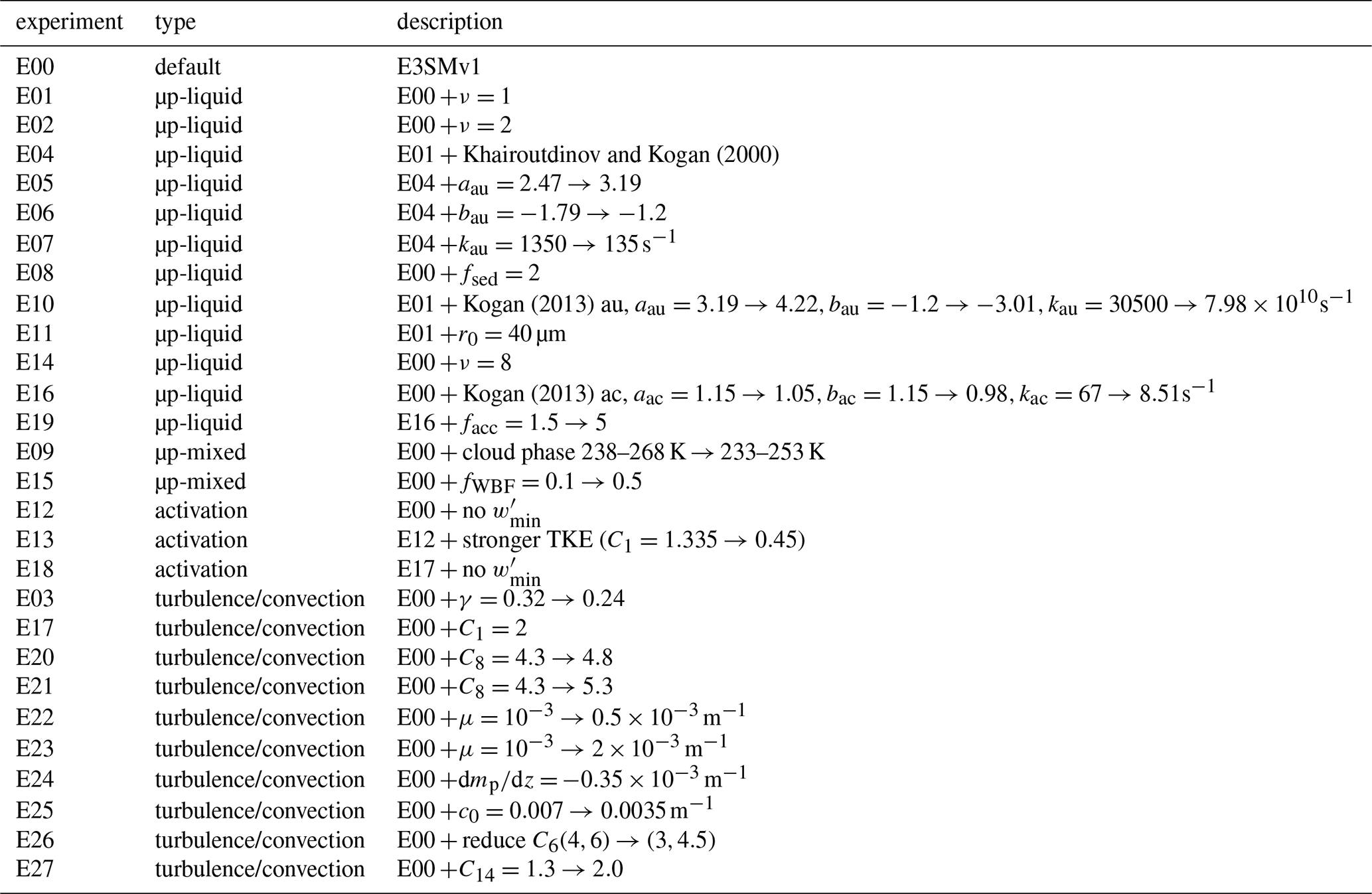
For µp-liquid, we first target the warm rain process, since previous studies suggest that autoconversion has strong control over the cloud “lifetime” effects (e.g., Rotstayn and Liu, 2005; Wang et al., 2012; Golaz et al., 2011; Suzuki et al., 2015; Mülmenstädt et al., 2020, 2021). Autoconversion is subject to large uncertainty because it is an artificial process intrinsic to the two-category bulk microphysics scheme to emulate the conversion from cloud to rain water due to collision–coalescence (Morrison et al., 2025; Mülmenstädt and Feingold, 2018). In addition to local autoconversion rate, the subgrid variability assumption, parameterized as the inverse relative variance of liquid-water mixing ratio ν, affects the total grid-box autoconversion rate by acting as an enhancement factor. While the Khairoutdinov and Kogan (2000) and Kogan (2013) parameterizations are developed for stratocumulus and shallow cumulus, respectively, Rasch et al. (2019) adjust the parameters for the local autoconversion rate and use ν predicted by CLUBB to provide acceptable results in various regimes across the globe (Ovchinnikov et al., 2024). Furthermore, the cutoff size r0 separating cloud and raindrops varies from 25 µm for stratocumulus (Khairoutdinov and Kogan, 2000) to 40 µm for trade shallow cumulus (Kogan, 2013). In µp-liquid, we test the sensitivity of the autoconversion (au) and accretion (ac) parameterizations, which take power-law forms in cloud-water mixing ratio qc, rain-water mixing ratio qr, and Nd:
We vary their parameters according to Khairoutdinov and Kogan (2000), Kogan (2013), and Rasch et al. (2019). We further perturb ν, r0, and an accretion enhancement factor facc that multiplies the right-hand side of Eq. (2). We also introduce an enhancement factor for cloud sedimentation fsed to test the sedimentation–entrainment feedback identified in Bretherton et al. (2007) that appears to control RAℒ in E3SM under certain conditions (Mülmenstädt et al., 2024b).
Cloud phase partitioning is important for ACIs, as it determines which mechanisms are active. Ensemble member E09 investigates the effects of increasing the liquid condensate amount by lowering the temperature range in which detrained water condensate from deep convection is treated as ice. In EAMv1, the ratio of liquid condensate over total condensate detrained from deep convection is 1 above 268 K, 0 below 238 K, and is linearly interpolated in between. Lowering the temperature thresholds increases liquid condensate amount in low latitudes and areas where the Zhang and McFarlane (1995) deep convection parameterization is triggered. Another experiment, E15, reduces ℒ by increasing a scale factor fWBF on the Wegener–Bergeron–Findeisen process from 0.1 to 0.5. As documented in Rasch et al. (2019) and Ma et al. (2022), the excessive liquid condensate amount in EAMv1 is attributable to the unrealistically low fWBF=0.1. Increasing fWBF reduces ℒ in mid and high latitudes.
Atmospheric turbulence affects ACIs directly through changing aerosol activation and indirectly through changing atmospheric state, including clouds and boundary layer structure. The six CLUBB parameters perturbed in the turbulence/convection group of experiments (γ, C1, C6, C8, C14, and μ) control how strong or skewed turbulence is and affect cloud formation and boundary layer structure. As discussed in depth by Ma et al. (2022), C1 damps vertical velocity variance (), so higher C1 leads to weaker vertical mixing and shallower boundary layer, which results in more persistent stratocumulus and less frequent decoupling of the cloud from the surface. Increasing C1 also reduces aerosol activation as updraft velocity weakens (E17). The γ parameter sets the width of the assumed subgrid vertical velocity (w′) PDF. Lowering γ results in a narrower PDF, which facilitates low-cloud formation and results in larger low-cloud fraction (E03). C8 damps the third moment of vertical velocity (), controlling the skewness of the vertical velocity PDF. Higher C8 leads to more symmetric, stratocumulus-like mixing (E20, E21). The μ parameter is a fractional entrainment rate. Decreasing/increasing μ leads to less/more plume dilution, resulting in higher/lower liquid condensate amount (E22/E23). C6 damps vertical scalar fluxes of total moisture and liquid water potential temperature . Reducing C6 leads to stronger fluxes, enabling a deeper, more decoupled boundary layer (E26). C14 damps horizontal velocity variances. Higher C14 results in weaker shear-driven turbulence and less entrainment, which leads to a shallower, more stratiform boundary layer with more low-level cloud. Similarly, the Zhang and McFarlane (1995) parameters affect how much condensate gets routed to cloud microphysics. Reducing c0 results in slower conversion of convective cloud water to rain, increasing both cloud condensate amount and droplet number (E25). Reducing the magnitude of fractional entrainment in the calculation of “dilute” convective available potential energy (Neale et al., 2008) strengthens deep convection, which decreases low-cloud ℒ (E24).
Lastly, to fully capture the effect of changing updraft velocity on aerosol activation, we remove the artificial limiter so that the full range of CLUBB-predicted values are used in aerosol activation parameterization (E12, E13, E18). These experiments form the “activation” group.
The EAMv1 model is configured to run at ne30np4 horizontal grid spacing (approximately 1 degree) with 72 levels in the vertical. EAMv1 simulations are performed with prescribed sea surface temperature (SST) and sea ice cover. The atmosphere is simulated by EAMv1 with horizontal winds nudged to agree with the Modern-Era Retrospective analysis for Research and Applications version 2 (MERRA-2; Gelaro et al., 2017) reanalysis with a 6 h relaxation timescale so that the aerosol forcing signals can be extracted from internal variability in short-duration model runs (Kooperman et al., 2012; Zhang et al., 2014). While the nudging eliminates any potential adjustments of the large-scale circulation to the aerosol forcing, we do not expect this to affect analysis of the local RAℒ mechanisms – precipitation suppression and cloud-top entrainment – of interest to this study. To assess aerosol ERF (Boucher et al., 2014; Sherwood et al., 2015), paired one-year simulations are performed for each ensemble member, with one driven by present-day emissions of aerosols and their precursors, and the other driven by preindustrial emissions (as in, e.g., Ghan et al., 2016).
2.2 Cloud selection
The cloud selection follows Mülmenstädt et al. (2024a): from the 3-hourly instantaneous model output, we select liquid clouds, defined by the absence of ice (ice cloud cover = 0) in the column. We require near-overcast (liquid cloud cover > 0.9) conditions for consistency with the Mülmenstädt et al. (2024a, b) analyses. Although the clouds are nearly overcast, we account for the remaining variability in cloud cover by calculating cloudy-sky cloud-top droplet number concentration Nd and cloudy-sky ℒ by dividing the grid-mean model outputs by the projected cloud cover.
2.3 Inverted-v Nd–ℒ relationship and estimate of curve shape
As in the Mülmenstädt et al. (2024a, b) analyses, we collapse the conditional probability distribution function P(ℒ|Nd) (Gryspeerdt et al., 2019) into the geometric-mean ℒ as a function of Nd to be able to compare multiple model variants more succinctly. The geometric mean is used because P(ℒ|Nd) is closer to lognormal than to normal.
Following Gryspeerdt et al. (2019), we further summarize the ℒ–Nd relationship by performing an ordinary least squares fit of an inverted v-shaped function (two linear segments meeting at an apex point) that results in a predicted (the caret denotes prediction) as a function of Nd:
The apex point is given by the coordinates in Nd–ℒ phase space, ml is the (usually positive) slope in the region, and mh is the (usually negative) slope in the region. This reduces the Nd–ℒ relationship to four shape variables per model experiment. The conventional interpretation of ml and mh is that they are fingerprints of the precipitation-suppression and enhanced-entrainment adjustment mechanisms, respectively, though this interpretation is overly simplified (e.g., Gryspeerdt et al., 2019; Mülmenstädt et al., 2024a; Goren et al., 2025), as discussed below. Like Gryspeerdt et al. (2019), we use unit weight for each Nd bin; this is done so the fit-derived mh can be constrained by the Gryspeerdt et al. (2019) observational mh.
2.4 Emergent constraint on
An emergent constraint (Hall and Qu, 2006; Klein and Hall, 2015) describes a statistical relationship linking an observable in the present-day climate with an unobservable emergent response of the climate system when an anthropogenic perturbation acts on the system. The emergent response is “unobservable” in the sense that we would like to know its value before the real climate system evolves into this state (e.g., future temperature) or because the emergent response corresponds to an idealization that is never realized in the physical system, such as the forcing–adjustments–feedbacks framework (Boucher et al., 2014; Sherwood et al., 2015; Quaas et al., 2024). Because the emergent response is unobservable, the statistical relationship is drawn from lines of evidence that can be used to estimate the emergent response, typically numerical climate models. Because some degree of model diversity is needed for statistical techniques (e.g., linear regression) to give precise (but not necessarily accurate) estimates of the statistical relationship, model ensembles, either MMEs or PPEs, are customarily used. If the statistical relationship is based on an underlying physical mechanism, rather than on spurious correlation or confounding, the statistical relationship can be used to constrain the unobservable emergent property.
Proposed emergent constraints on the climatic effects of anthropogenic aerosols (Quaas et al., 2009; Wang et al., 2012; Mülmenstädt and Feingold, 2018) relate the components of ERF from ACIs as unobservable emergent properties of the climate to aerosol susceptibilites of cloud properties in the present-day internal variability as observables. The underlying hypothesis is that the physical mechanisms behind the climatic response of clouds to the anthropogenic aerosol perturbation are also, at least in part, responsible for the observed correlations between clouds and aerosols in the present day. In our case, the emergent climate response we seek to constrain is the ratio of ℒPD in the present day to ℒPI under a preindustrial emissions scenario, . This anthropogenic perturbation in ℒ is closely linked to the radiative adjustment RAℒ (Gryspeerdt et al., 2020; Duran et al., 2026). The observables in the present day are the slope ml and mh of the the Nd–ℒ relationship, defined in Eq. (3) above, for which a satellite-based estimate exists (Gryspeerdt et al., 2019). Recent-generation GCMs produce an inverted-v Nd–ℒ relationship, unlike older GCMs, in which ℒ monotonically increases with Nd (Mülmenstädt et al., 2024a). This recently manifested agreement motivates investigating an mh-based emergent constraint, which would hold limited promise when models and observations disagree on its sign. The statistical relationship investigated is a linear relationship between and ml or mh, whose parameters are estimated by performing a linear regression on the PPE members.
Note that instead of the difference , we use the ratio (or, equivalently for Δℒ≪ℒ, the logarithmic difference ). We do so for two reasons. First, Δlog ℒ performs well as a proxy for RAℒ across a range of base-state ℒ (Duran et al., 2026). Second, the climate response is a function of the base state, which in these experiments is not constrained to the observed base state (e.g., Elsaesser et al., 2025; Wynn et al., 2026). While normalizing to the base state ℒ is far from perfect (e.g., Mülmenstädt et al., 2020, and see discussion below), it at least removes the first-order (proportional) relationship between the base state and the perturbation.
3.1 Inverted v and anthropogenic change in ℒ across PPE members
Figure 1 shows the Nd–ℒ relationships of the PPE member with the most negatively sloped inverted v (E05), the default EAMv1 PPE member (E00), and the PPE member with the least negatively sloped inverted v (E10, which is also the only PPE member with mh≥0). It is clear in Fig. 1 that the turnover in slope occurs markedly more gradually in the models than the inverted-v fit function can capture. Nevertheless, both positive and negative slopes away from the apex appear well captured. Neither the residual sum of squares – a goodness of fit metric – nor the fit uncertainty σ(mh) of the descending slope is strongly correlated with mh. Nor does either depend strongly on the experiment type (Figs. S1 and S2 in the Supplement). It is therefore unlikely that the use of mh in an emergent constraint is biased by artifacts of the fit procedure. We choose to retain the inverted-v fit function for its simplicity and small number of shape variables.
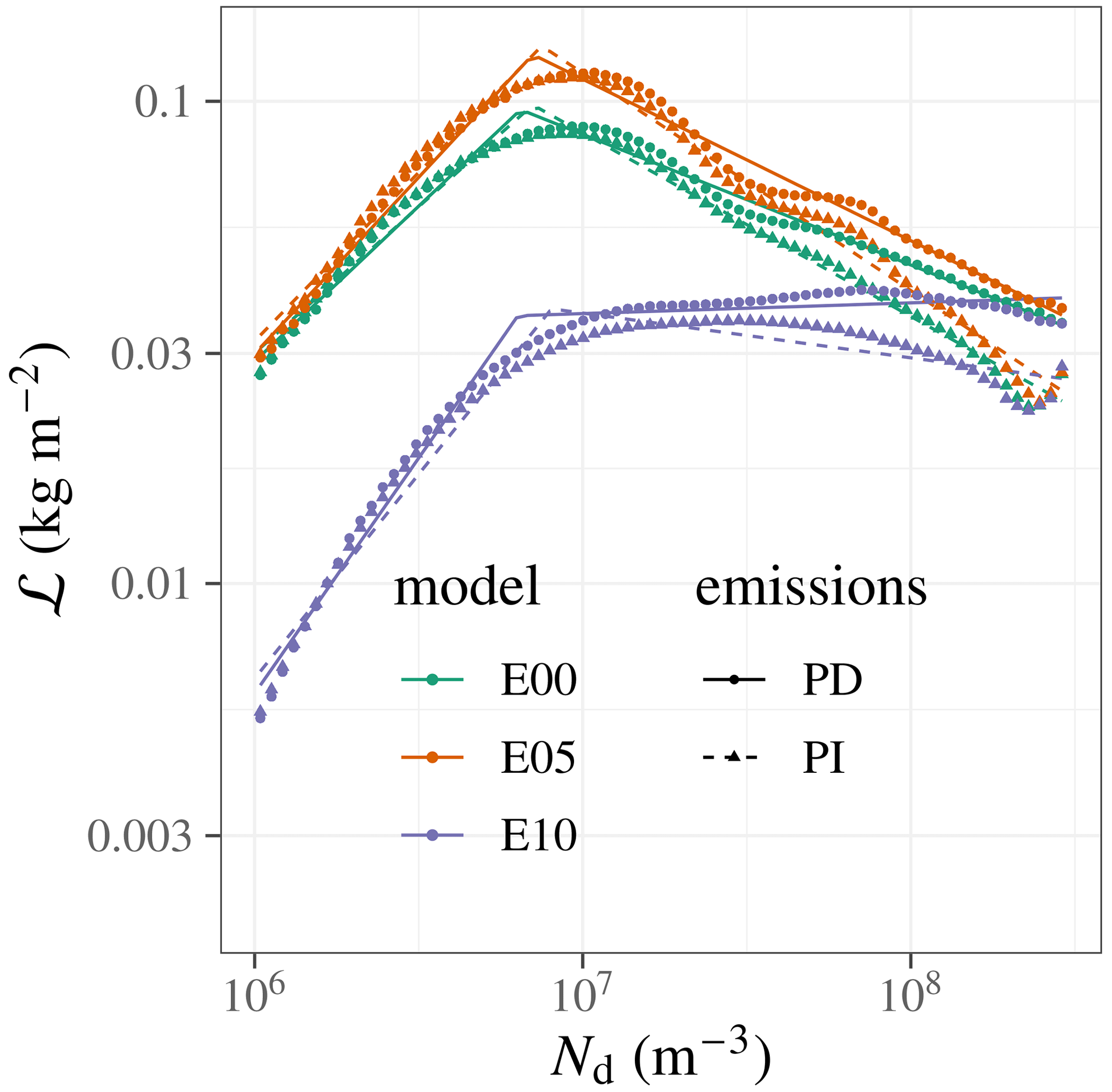
Figure 1Nd–ℒ relationships across PPE members. Default model configuration and configurations with the most negative and least negative descending-leg slope are shown. Inverted-v fits are overlaid. Present day (PD) and preindustrial (PI) emissions scenarios are shown.
Figure 2 shows histograms of mh, , and their scatter. As noted in the previous paragraph, all PPE members but one produce an inverted-v-shaped Nd–ℒ relationship, that is, ml>0 and mh<0. All PPE members but one produce higher ℒ with present-day emissions than with preindustrial emissions, and even the PPE member with , E05, only shows a minute anthropogenic decrease in ℒ ( −3.1 ). The PPE members thus behave similarly to the E3SM results of Christensen et al. (2023) and Varble et al. (2023), MME described by Mülmenstädt et al. (2024a), and Community Atmosphere Model version 6 (CAM6) PPE described by Mikkelsen et al. (2025): robust negative slopes in the Nd–ℒ relationship but no sign of an appreciable global-mean decrease in ℒ due to anthropogenic Nd perturbation.
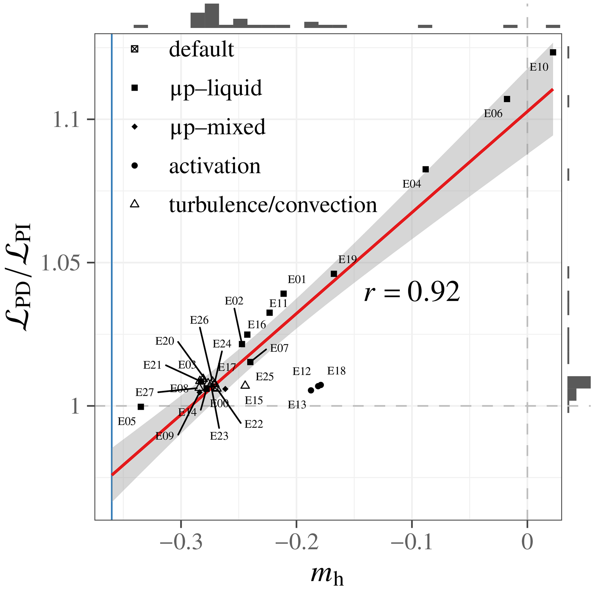
Figure 2Scatter of mh against and marginal distributions of mh and across PPE members. Physics perturbation labels are as in Table 1. The satellite-derived value of mh reported by Gryspeerdt et al. (2019) is indicated as a vertical line. The emergent constraint using the PPE regression and the Gryspeerdt et al. (2019) satellite-observed mh is (90 % interval calculated from the regression standard error).
3.2 Parametric controls on and mh
Both and mh differ markedly between the four groups of perturbations that constitute the PPE:
- Liquid microphysics
-
Both mh and respond more strongly to liquid microphysical parameters than to any other group of parameters perturbed in the PPE. This is especially true for precipitation-related parameters. The responses of mh and to precipitation parameters are highly correlated, driving the overall regression of onto mh and the overall high correlation (r=0.92) between and mh.
A strong response of to the precipitation parameters is expected given the central role of precipitation suppression in the model's RAℒ. What is less expected is that the correlation is between and mh, not ml (shown in Fig. S3), when process understanding tells us that ml is the leg of the inverted v that reflects precipitation suppression. One possible explanation is that the negative correlation is intrinsic (due, for example, to confounding by circulation or precipitation; Mülmenstädt et al., 2024a; Mikkelsen et al., 2026), but precipitation suppression rotates the entire Nd–ℒ relationship, even at high Nd, toward less negative values of the regression slope. In this interpretation, a possible explanation for the absence of a correlation between and ml could be that ml is not actually a process fingerprint for precipitation suppression, as suggested by Goren et al. (2025). Additionally, the apex point in the model occurs at a very low cm−3 compared with observations ( cm−3); consequently, the ml regression is driven by the comparably small number of events at very low Nd, which may reduce its usefulness.
Precipitation affects ℒ directly by removing moisture from the cloudy boundary layer, but it also decreases the kinetic energy of the boundary layer circulation through its effect on the vertical structure of latent heating (Stevens et al., 1998), leading to a decrease in cloud-top entrainment (Ackerman et al., 2004). Precipitation suppression can therefore increase entrainment and thus decrease ℒ, particularly in drizzling cloud (e.g., Ackerman et al., 2004; Hoffmann et al., 2025). It is plausible that precipitation suppression, in turn, is strongly dependent on the precipitation parameterization, which could explain why mh varies so strongly across the precipitation experiments.
The effect of the precipitation parameters on need not be only through the precipitation suppression mechanism. In addition to an effect of Nd on precipitation, there are also effects of precipitation on Nd, for example, via scavenging (Wood et al., 2012; Gryspeerdt et al., 2019; McCoy et al., 2020; Mikkelsen et al., 2025). Indeed, many of the PPE members with large changes relative to the default model also show large correlated changes (Fig. S4). Part of the explanation for the dependence on precipitation may thus simply be the effect of precipitation on Nd. We emphasize that it is not likely to explain the entire dependence: the tightest (most correlated) relationship is still between and mh, not or base-state Nd, counter to what we would expect if the precipitation effect on Nd explained the precipitation effect on .
The Nd exponent in autoconversion (bau) does not appear to play any special role compared with other autoconversion parameters, evidenced by E05, E06, and E07 all falling on a common line with the other warm-cloud microphysics PPE members. Since bau also changes the base-state precipitation probability, this provides further evidence that precipitation probability, rather than precipitation susceptibility, controls the global RAℒ, as also reported for the ECHAM–HAM model by Mülmenstädt et al. (2020). (This conclusion applies to the values of bau typically used in tuned two-moment microphysics schemes in GCMs. At some point, the precipitation-suppression contribution to RAℒ must go to zero as bau→0 (Gryspeerdt et al., 2020; Mahfouz et al., 2024; Mülmenstädt et al., 2024b), but in the −1.2 range explored in this PPE, we are apparently far from this change in behavior.)
- Mixed-phase microphysics
-
The mixed-phase microphysical parameters perturbed in this ensemble do not appear to have a strong effect on the anthropogenic change in ℒ in the purely liquid clouds selected for analysis.
- Turbulence and convection
-
Neither convection nor turbulence parameter perturbations cause appreciable changes in or mh. Given the process interpretation that the descending branch of the inverted v is controlled by turbulence-mediated entrainment feedbacks, the absence of a response to turbulence parameters is surprising. If an entrainment feedback is active in the model, as Mülmenstädt et al. (2024b) argue, it is either not sensitive to the turbulence parameters or of negligible significance in the global mean. That mh is insensitive to turbulence parameters and negative is further evidence that the negative correlation between Nd and ℒ is primarily driven by mechanisms other than microphysical adjustment processes (Mülmenstädt et al., 2024a; Goren et al., 2025).
- Activation
-
The PPE members with perturbed activation form a cluster apart from the other PPE members in mh– space. Their is comparable to the other PPE members with default microphysics (i.e., not in the µp-liquid group). However, a higher (less negative) mh sets these experiments apart from the other group of experiments without change. The mechanism for either behavior is unclear. Both base-state Nd and differ across the three activation experiments (Figs. S4 and S5), indicating that the absence of a response in is likely due to compensation between multiple mechanisms.
3.3 Potential emergent constraint on from the slope of the inverted v
The PPE relationship between mh, which is observable in the present day, and , an unobservable climate response, qualifies as a candidate for an emergent constraint. Read as an emergent constraint, a linear regression based on the PPE members can be used to infer a constrained corresponding to the observed satellite value (Gryspeerdt et al., 2019). The constrained (90 % interval calculated from the regression standard error), which would bring the sign of the emergent-constraint-based GCM estimate into agreement with other lines of evidence on RAℒ (Bellouin et al., 2020).
Klein and Hall (2015) warn that candidates for emergent constraints must be thoroughly vetted to distinguish a true emergent constraint – with actual predictive power for the unobservable climate response – from undesirable correlations that occur for reasons other than a mechanistic link between the present-day observable and the climate response. In general, it is not possible to rule out such reasons, which can include spurious correlations that are an accident of statistical sampling or mechanistic links other than the hypothesized mechanism but with no bearing on the climate response. Evidence in favor of the emergent constraint relationship identified here falls into two categories identified by Klein and Hall (2015). First, the correlation between the observable and the climate response is strong, reducing the risk of a spurious correlation. Second, the candidate emergent constraint relationship results from perturbations to the model representation of physical processes (precipitation, turbulence) that are hypothesized to affect both the present-day observable and the climate response; as Klein and Hall (2015) point out, the use of a PPE provides a more direct attribution of the emergent constraint to physics perturbations than an MME would.
As with any emergent constraint candidate, confidence will grow if these results are replicated in other model ensembles. In part, this is because replication increases statistical robustness. More importantly, investigating this emergent constraint candidate in other host models or with other cloud, precipitation, and turbulence parameterizations means the hypothesized underlying model mechanisms will be structurally perturbed, resulting in more robust attribution of the emergent constraint response to these mechanisms.
There is an additional test, more specific to this emergent constraint candidate, that would help distinguish between two very different types of statistical relationships. In the first, the relationship between the observable and the climate response exists only because both depend on the base state (e.g., Mülmenstädt et al., 2020). This type of relationship is of no use in the real climate projection problem, where the base state is given; ignoring the base-state constraint results in misleading conclusions about sensitivities to climate perturbations (Wynn et al., 2026). In the second type of statistical relationship, the relationship exists even when the base state is held fixed, as is the case in the climate projection problem. We normalize to base-state ℒ in our analysis to reduce the danger of reporting on a relationship of the first kind. In PPEs of cloud and turbulence parameters with emulators (e.g., Regayre et al., 2023; Eidhammer et al., 2024; Elsaesser et al., 2025; Nugent et al., 2026; Wynn et al., 2026), it would be possible to perform this test more conclusively by determining whether the emergent constrain candidate presented here persists when the constraint of the present-day observable climate state is imposed to reduce the accessible model parameter space.
Modern GCMs are able (Mülmenstädt et al., 2024a) to reproduce the negative relationship between Nd and ℒ seen in satellite retrievals (Gryspeerdt et al., 2019) and large eddy simulations (e.g., Glassmeier et al., 2019; Hoffmann et al., 2020). Nonetheless, GCMs predict that , that is, the causal effect of an increase in Nd is to increase ℒ, the opposite sign of the correlation observed in present-day internal variability. Mülmenstädt et al. (2024a, b) argue that this raises the troubling possibility that we are misinterpreting the observational and large eddy simulation (LES) lines of evidence due to the difficulty of establishing causality in observations and the difficulty of determining whether the idealized or sporadic cases that have been simulated by LES are representative of the global climate behavior.
Perhaps we can now see a few more shades of gray between these two categorical extremes. Instead of asking binary questions such as “is the negative correlation between Nd and ℒ causal?” (Mülmenstädt et al., 2024a), we can instead ask whether the slope, as a continuous variable, provides a continuous constraint on the adjustment mechanism. The answer to this quantitative, rather than categorical, question appears to be affirmative. It also appears to resolve some of the tension between Mülmenstädt et al. (2024a) and other lines of evidence on RAℒ; the mere existence of a negative slope is not a guarantee of , but a negative-enough slope, including the satellite-observed , does indicate . A simple model to explain this behavior is that the present-day Nd–ℒ relationship is the result of ACI mechanisms that contribute to RAℒ and confounders that do not depend on anthropogenic aerosols and therefore do not contribute to RAℒ. If these contributions to mh are additive (an assumption that is reflected in the choice of a linear emergent-constraint relationship between mh and ), then mh can be used as a predictor for RAℒ by subtracting the “confounded” mh contribution to reveal the “causal” component of mh.
The other binary question we have asked previously, “is the model structurally capable of representing adjustment mechanisms that reduce ℒ?” (Mülmenstädt et al., 2024b), nevertheless remains. One interpretation of the existence of this emergent constraint relationship is that there is a parametric explanation for the differences between the GCM estimate of RAℒ and the estimate from other lines of evidence; that is, the model could in principle be tuned to produce . This interpretation is also consistent with the finding that an enhanced entrainment mechanism is represented and active in the model (Mülmenstädt et al., 2024b) but is neither the dominant RAℒ mechanism nor the dominant contributor to the negative Nd–ℒ correlation. This parametric explanation is in conflict, however, with the absence of any PPE members that convincingly produce and with the very muted response of and mh to turbulence parameters. Whether global models are structurally capable of agreement with other lines of evidence on RAℒ is therefore still a question looking for a definitive answer.
Model output is available from https://doi.org/10.5281/zenodo.18512978 (Ma and Mülmenstädt, 2026). The analysis code is available from https://doi.org/10.5281/zenodo.18513015 (Mülmenstädt, 2026). The analysis code relies on an R package available from https://doi.org/10.5281/zenodo.14286144 (Mülmenstädt, 2024).
The supplement related to this article is available online at https://doi.org/10.5194/acp-26-16465-2026-supplement.
Both authors contributed to the experiment design, model runs, data analysis, or manuscript writing.
The contact author has declared that neither of the authors has any competing interests.
Publisher's note: Copernicus Publications remains neutral with regard to jurisdictional claims made in the text, published maps, institutional affiliations, or any other geographical representation in this paper. The authors bear the ultimate responsibility for providing appropriate place names. Views expressed in the text are those of the authors and do not necessarily reflect the views of the publisher.
We thank Yi Qin for discussion of the methods, results, and manuscript. We thank Christina Sackmann and the anonymous reviewers for suggestions that improved the manuscript.
This study was supported as part of the Enabling Aerosol–cloud interactions at GLobal convection-permitting scalES (EAGLES) project (project no. 74358) sponsored by the United States Department of Energy (DOE), Office of Science, Office of Biological and Environmental Research (BER), Earth System Model Development (ESMD), and Regional and Global Model Analysis (RGMA) program areas. Pacific Northwest National Laboratory (PNNL) is operated for the DOE by the Battelle Memorial Institute under Contract DE-AC05-76RL01830. The research used high-performance computing resources of the National Energy Research Scientific Computing Center (NERSC), a U.S. DOE Office of Science User Facility located at Lawrence Berkeley National Laboratory, operated under Contract DE-AC02-05CH11231, using NERSC awards BER-ERCAP0029295, BER-ERCAP0024471, and BER-ERCAP0033555.
This paper was edited by Guy Dagan and reviewed by four anonymous referees.
Abdul-Razzak, H. and Ghan, S. J.: A parameterization of aerosol activation 2. Multiple aerosol types, J. Geophys. Res., 105, 6837–6844, https://doi.org/10.1029/1999JD901161, 2000. a
Ackerman, A., Kirkpatrick, M., Stevens, D., and Toon, O.: The impact of humidity above stratiform clouds on indirect aerosol climate forcing, Nature, 432, 1014–1017, https://doi.org/10.1038/nature03174, 2004. a, b, c
Albrecht, B. A.: Aerosols, Cloud Microphysics, and Fractional Cloudiness, Science, 245, 1227–1230, 1989. a
Bellouin, N., Quaas, J., Gryspeerdt, E., Kinne, S., Stier, P., Watson-Parris, D., Boucher, O., Carslaw, K. S., Christensen, M., Daniau, A.-L., Dufresne, J.-L., Feingold, G., Fiedler, S., Forster, P., Gettelman, A., Haywood, J. M., Lohmann, U., Malavelle, F., Mauritsen, T., McCoy, D. T., Myhre, G., Mülmenstädt, J., Neubauer, D., Possner, A., Rugenstein, M., Sato, Y., Schulz, M., Schwartz, S. E., Sourdeval, O., Storelvmo, T., Toll, V., Winker, D., and Stevens, B.: Bounding Global Aerosol Radiative Forcing of Climate Change, Rev. Geophys., 58, e2019RG000660, https://doi.org/10.1029/2019RG000660, 2020. a, b, c, d
Boucher, O., Randall, D., Artaxo, P., Bretherton, C., Feingold, G., Forster, P., Kerminen, V.-M., Kondo, Y., Liao, H., Lohmann, U., Rasch, P., Satheesh, S., Sherwood, S., Stevens, B., and Zhang, X.: Clouds and Aerosols, book section Chapter 7, Cambridge University Press, Cambridge, United Kingdom and New York, NY, USA, 571–658, ISBN 978-1-107-66182-0, https://doi.org/10.1017/CBO9781107415324.016, 2014. a, b, c, d
Bretherton, C. S., Blossey, P. N., and Uchida, J.: Cloud droplet sedimentation, entrainment efficiency, and subtropical stratocumulus albedo, Geophys. Res. Lett., 34, https://doi.org/10.1029/2006GL027648, 2007. a, b
Christensen, M. W., Ma, P.-L., Wu, P., Varble, A. C., Mülmenstädt, J., and Fast, J. D.: Evaluation of aerosol–cloud interactions in E3SM using a Lagrangian framework, Atmos. Chem. Phys., 23, 2789–2812, https://doi.org/10.5194/acp-23-2789-2023, 2023. a
Duran, B. M., Wall, C. J., Lutsko, N. J., Wynn, S., Watson-Parris, D., and Mülmenstädt, J.: A new proxy for the LWP adjustment from first principles, ESS Open Archive [preprint], https://doi.org/10.22541/essoar.15006786/v1, 2026. a, b
Eidhammer, T., Gettelman, A., Thayer-Calder, K., Watson-Parris, D., Elsaesser, G., Morrison, H., van Lier-Walqui, M., Song, C., and McCoy, D.: An extensible perturbed parameter ensemble for the Community Atmosphere Model version 6, Geosci. Model Dev., 17, 7835–7853, https://doi.org/10.5194/gmd-17-7835-2024, 2024. a
Elsaesser, G. S., van Lier-Walqui, M., Yang, Q., Kelley, M., Ackerman, A. S., Fridlind, A. M., Cesana, G. V., Schmidt, G. A., Wu, J., Behrangi, A., Camargo, S. J., De, B., Inoue, K., Leitmann-Niimi, N. M., and Strong, J. D. O.: Using Machine Learning to Generate a GISS ModelE Calibrated Physics Ensemble (CPE), J. Adv. Model. Earth Sy., 17, e2024MS004713, https://doi.org/10.1029/2024MS004713, 2025. a, b
Forster, P., Storelvmo, T., Armour, K., Collins, W., Dufresne, J.-L., Frame, D., Lunt, D., Mauritsen, T., Palmer, M., Watanabe, M., Wild, M., and Zhang, H.: The Earth’s Energy Budget, Climate Feedbacks, and Climate Sensitivity, Chap. 7, Cambridge University Press, 923–1054, https://doi.org/10.1017/9781009157896.009, 2021. a, b, c
Gelaro, R., McCarty, W., Suarez, M. J., Todling, R., Molod, A., Takacs, L., Randles, C. A., Darmenov, A., Bosilovich, M. G., Reichle, R., Wargan, K., Coy, L., Cullather, R., Draper, C., Akella, S., Buchard, V., Conaty, A., da Silva, A. M., Gu, W., Kim, G.-K., Koster, R., Lucchesi, R., Merkova, D., Nielsen, J. E., Partyka, G., Pawson, S., Putman, W., Rienecker, M., Schubert, S. D., Sienkiewicz, M., and Zhao, B.: The Modern-Era Retrospective Analysis for Research and Applications, Version 2 (MERRA-2), J. Climate, 30, 5419–5454, https://doi.org/10.1175/JCLI-D-16-0758.1, 2017. a
Gettelman, A. and Morrison, H.: Advanced Two-Moment Bulk Microphysics for Global Models. Part I: Off-Line Tests and Comparison with Other Schemes, J. Climate, 28, 1268–1287, https://doi.org/10.1175/JCLI-D-14-00102.1, 2015. a
Gettelman, A., Morrison, H., Santos, S., Bogenschutz, P., and Caldwell, P. M.: Advanced Two-Moment Bulk Microphysics for Global Models. Part II: Global Model Solutions and Aerosol-Cloud Interactions, J. Climate, 28, 1288–1307, https://doi.org/10.1175/JCLI-D-14-00103.1, 2015. a
Ghan, S., Wang, M., Zhang, S., Ferrachat, S., Gettelman, A., Griesfeller, J., Kipling, Z., Lohmann, U., Morrison, H., Neubauer, D., Partridge, D. G., Stier, P., Takemura, T., Wang, H., and Zhang, K.: Challenges in constraining anthropogenic aerosol effects on cloud radiative forcing using present-day spatiotemporal variability, P. Natl. Acad. Sci. USA, 113, 5804–5811, https://doi.org/10.1073/pnas.1514036113, 2016. a
Glassmeier, F., Hoffmann, F., Johnson, J. S., Yamaguchi, T., Carslaw, K. S., and Feingold, G.: An emulator approach to stratocumulus susceptibility, Atmos. Chem. Phys., 19, 10191–10203, https://doi.org/10.5194/acp-19-10191-2019, 2019. a
Golaz, J.-C., Salzmann, M., Donner, L. J., Horowitz, L. W., Ming, Y., and Zhao, M.: Sensitivity of the Aerosol Indirect Effect to Subgrid Variability in the Cloud Parameterization of the GFDL Atmosphere General Circulation Model AM3, J. Climate, 24, 3145–3160, https://doi.org/10.1175/2010JCLI3945.1, 2011. a
Golaz, J.-C., Caldwell, P. M., Van Roekel, L. P., Petersen, M. R., Tang, Q., Wolfe, J. D., Abeshu, G., Anantharaj, V., Asay-Davis, X. S., Bader, D. C., Baldwin, S. A., Bisht, G., Bogenschutz, P. A., Branstetter, M., Brunke, M. A., Brus, S. R., Burrows, S. M., Cameron-Smith, P. J., Donahue, A. S., Deakin, M., Easter, R. C., Evans, K. J., Feng, Y., Flanner, M., Foucar, J. G., Fyke, J. G., Griffin, B. M., Hannay, C., Harrop, B. E., Hoffman, M. J., Hunke, E. C., Jacob, R. L., Jacobsen, D. W., Jeffery, N., Jones, P. W., Keen, N. D., Klein, S. A., Larson, V. E., Leung, L. R., Li, H.-Y., Lin, W., Lipscomb, W. H., Ma, P.-L., Mahajan, S., Maltrud, M. E., Mametjanov, A., McClean, J. L., McCoy, R. B., Neale, R. B., Price, S. F., Qian, Y., Rasch, P. J., Eyre, J. E. J. R., Riley, W. J., Ringler, T. D., Roberts, A. F., Roesler, E. L., Salinger, A. G., Shaheen, Z., Shi, X., Singh, B., Tang, J., Taylor, M. A., Thornton, P. E., Turner, A. K., Veneziani, M., Wan, H., Wang, H., Wang, S., Williams, D. N., Wolfram, P. J., Worley, P. H., Xie, S., Yang, Y., Yoon, J.-H., Zelinka, M. D., Zender, C. S., Zeng, X., Zhang, C., Zhang, K., Zhang, Y., Zheng, X., Zhou, T., and Zhu, Q.: The DOE E3SM Coupled Model Version 1: Overview and Evaluation at Standard Resolution, J. Adv. Model. Earth Sy., 11, 2089–2129, https://doi.org/10.1029/2018MS001603, 2019. a
Goren, T., Choudhury, G., Kretzschmar, J., and McCoy, I.: Co-variability drives the inverted-V sensitivity between liquid water path and droplet concentrations, Atmos. Chem. Phys., 25, 3413–3423, https://doi.org/10.5194/acp-25-3413-2025, 2025. a, b, c
Gryspeerdt, E., Goren, T., Sourdeval, O., Quaas, J., Mülmenstädt, J., Dipu, S., Unglaub, C., Gettelman, A., and Christensen, M.: Constraining the aerosol influence on cloud liquid water path, Atmos. Chem. Phys., 19, 5331–5347, https://doi.org/10.5194/acp-19-5331-2019, 2019. a, b, c, d, e, f, g, h, i, j, k
Gryspeerdt, E., Mülmenstädt, J., Gettelman, A., Malavelle, F. F., Morrison, H., Neubauer, D., Partridge, D. G., Stier, P., Takemura, T., Wang, H., Wang, M., and Zhang, K.: Surprising similarities in model and observational aerosol radiative forcing estimates, Atmos. Chem. Phys., 20, 613–623, https://doi.org/10.5194/acp-20-613-2020, 2020. a, b, c
Guo, H., Golaz, J.-C., and Donner, L. J.: Aerosol effects on stratocumulus water paths in a PDF-based parameterization, Geophys. Res. Lett., 38, L17808, https://doi.org/10.1029/2011GL048611, 2011. a
Guo, H., Golaz, J.-C., Donner, L. J., Ginoux, P., and Hemler, R. S.: Multivariate Probability Density Functions with Dynamics in the GFDL Atmospheric General Circulation Model: Global Tests, J. Climate, 27, 2087–2108, https://doi.org/10.1175/JCLI-D-13-00347.1, 2014. a
Hall, A. and Qu, X.: Using the current seasonal cycle to constrain snow albedo feedback in future climate change, Geophys. Res. Lett., 33, L03502, https://doi.org/10.1029/2005GL025127, 2006. a
Hoffmann, F., Glassmeier, F., Yamaguchi, T., and Feingold, G.: Liquid Water Path Steady States in Stratocumulus: Insights from Process-Level Emulation and Mixed-Layer Theory, J. Atmos. Sci., 77, 2203–2215, https://doi.org/10.1175/JAS-D-19-0241.1, 2020. a
Hoffmann, F., Chen, Y.-S., and Feingold, G.: On the processes determining the slope of cloud water adjustments in weakly and non-precipitating stratocumulus, Atmos. Chem. Phys., 25, 8657–8670, https://doi.org/10.5194/acp-25-8657-2025, 2025. a
Karset, I. H. H., Gettelman, A., Storelvmo, T., Alterskjaer, K., and Berntsen, T. K.: Exploring Impacts of Size-Dependent Evaporation and Entrainment in a Global Model, J. Geophys. Res., 125, e2019JD031817, https://doi.org/10.1029/2019JD031817, 2020. a
Khairoutdinov, M. and Kogan, Y.: A new cloud physics parameterization in a large-eddy simulation model of marine stratocumulus, Mon. Weather Rev., 128, 229–243, https://doi.org/10.1175/1520-0493(2000)128<0229:ANCPPI>2.0.CO;2, 2000. a, b, c, d
Klein, S. A. and Hall, A.: Emergent Constraints for Cloud Feedbacks, Current Climate Change Reports, 1, 276–287, https://doi.org/10.1007/s40641-015-0027-1, 2015. a, b, c, d, e, f
Kogan, Y.: A Cumulus Cloud Microphysics Parameterization for Cloud-Resolving Models, J. Atmos. Sci., 70, 1423–1436, https://doi.org/10.1175/JAS-D-12-0183.1, 2013. a, b, c, d, e
Kooperman, G. J., Pritchard, M. S., Ghan, S. J., Wang, M., Somerville, R. C. J., and Russell, L. M.: Constraining the influence of natural variability to improve estimates of global aerosol indirect effects in a nudged version of the Community Atmosphere Model 5, J. Geophys. Res., 117, D23204, https://doi.org/10.1029/2012JD018588, 2012. a
Liu, X., Ma, P.-L., Wang, H., Tilmes, S., Singh, B., Easter, R. C., Ghan, S. J., and Rasch, P. J.: Description and evaluation of a new four-mode version of the Modal Aerosol Module (MAM4) within version 5.3 of the Community Atmosphere Model, Geosci. Model Dev., 9, 505–522, https://doi.org/10.5194/gmd-9-505-2016, 2016. a
Ma, P.-L. and Mülmenstädt, J.: EAMv1 turbulence and microphysics PPE, Zenodo [data set], https://doi.org/10.5281/zenodo.18512978, 2026. a
Ma, P.-L., Harrop, B. E., Larson, V. E., Neale, R. B., Gettelman, A., Morrison, H., Wang, H., Zhang, K., Klein, S. A., Zelinka, M. D., Zhang, Y., Qian, Y., Yoon, J.-H., Jones, C. R., Huang, M., Tai, S.-L., Singh, B., Bogenschutz, P. A., Zheng, X., Lin, W., Quaas, J., Chepfer, H., Brunke, M. A., Zeng, X., Mülmenstädt, J., Hagos, S., Zhang, Z., Song, H., Liu, X., Pritchard, M. S., Wan, H., Wang, J., Tang, Q., Caldwell, P. M., Fan, J., Berg, L. K., Fast, J. D., Taylor, M. A., Golaz, J.-C., Xie, S., Rasch, P. J., and Leung, L. R.: Better calibration of cloud parameterizations and subgrid effects increases the fidelity of the E3SM Atmosphere Model version 1, Geosci. Model Dev., 15, 2881–2916, https://doi.org/10.5194/gmd-15-2881-2022, 2022. a, b, c
Mahfouz, N., Mülmenstädt, J., and Burrows, S.: Present-day correlations are insufficient to predict cloud albedo change by anthropogenic aerosols in E3SM v2, Atmos. Chem. Phys., 24, 7253–7260, https://doi.org/10.5194/acp-24-7253-2024, 2024. a
McCoy, D. T., Field, P., Gordon, H., Elsaesser, G. S., and Grosvenor, D. P.: Untangling causality in midlatitude aerosol–cloud adjustments, Atmos. Chem. Phys., 20, 4085–4103, https://doi.org/10.5194/acp-20-4085-2020, 2020. a
Mikkelsen, A., McCoy, D. T., Eidhammer, T., Gettelman, A., Song, C., Gordon, H., and McCoy, I. L.: Constraining aerosol–cloud adjustments by uniting surface observations with a perturbed parameter ensemble, Atmos. Chem. Phys., 25, 4547–4570, https://doi.org/10.5194/acp-25-4547-2025, 2025. a, b
Mikkelsen, A., McCoy, D. T., Nugent, J. M., Mülmenstädt, J., and Gordon, H.: Clarifying cloud liquid response to aerosol by accounting for precipitation, ESS Open Archive [preprint], https://doi.org/10.22541/essoar.176990469.97745860/v1, 2026. a
Morrison, H., Ma, P.-L., Geiss, A., Igel, A. L., Hu, A. Z., and van Lier-Walqui, M.: Impacts of Bulk Microphysics Scheme Structural Choices on Simulations of Rain Initiation Through Drop Coalescence, J. Adv. Model. Earth Sy., 17, e2025MS005026, https://doi.org/10.1029/2025MS005026, 2025. a
Mülmenstädt, J. and Feingold, G.: The radiative forcing of aerosol–cloud interactions in liquid clouds: Wrestling and embracing uncertainty, Current Climate Change Reports, 4, 23–40, https://doi.org/10.1007/s40641-018-0089-y, 2018. a, b
Mülmenstädt, J., Gryspeerdt, E., Salzmann, M., Ma, P.-L., Dipu, S., and Quaas, J.: Separating radiative forcing by aerosol–cloud interactions and rapid cloud adjustments in the ECHAM–HAMMOZ aerosol–climate model using the method of partial radiative perturbations, Atmos. Chem. Phys., 19, 15415–15429, https://doi.org/10.5194/acp-19-15415-2019, 2019. a
Mülmenstädt, J., Nam, C., Salzmann, M., Kretzschmar, J., L'Ecuyer, T. S., Lohmann, U., Ma, P.-L., Myhre, G., Neubauer, D., Stier, P., Suzuki, K., Wang, M., and Quaas, J.: Reducing the aerosol forcing uncertainty using observational constraints on warm rain processes, Science Adv., 6, eaaz6433, https://doi.org/10.1126/sciadv.aaz6433, 2020. a, b, c, d
Mülmenstädt, J., Salzmann, M., Kay, J. E., Zelinka, M. D., Ma, P.-L., Nam, C., Kretzschmar, J., Hörnig, S., and Quaas, J.: An underestimated negative cloud feedback from cloud lifetime changes, Nat. Clim. Change, 11, 508–513, https://doi.org/10.1038/s41558-021-01038-1, 2021. a
Mülmenstädt, J., Gryspeerdt, E., Dipu, S., Quaas, J., Ackerman, A. S., Fridlind, A. M., Tornow, F., Bauer, S. E., Gettelman, A., Ming, Y., Zheng, Y., Ma, P.-L., Wang, H., Zhang, K., Christensen, M. W., Varble, A. C., Leung, L. R., Liu, X., Neubauer, D., Partridge, D. G., Stier, P., and Takemura, T.: General circulation models simulate negative liquid water path–droplet number correlations, but anthropogenic aerosols still increase simulated liquid water path, Atmos. Chem. Phys., 24, 7331–7345, https://doi.org/10.5194/acp-24-7331-2024, 2024a. a, b, c, d, e, f, g, h, i, j, k, l, m
Mülmenstädt, J., Ackerman, A. S., Fridlind, A. M., Huang, M., Ma, P.-L., Mahfouz, N., Bauer, S. E., Burrows, S. M., Christensen, M. W., Dipu, S., Gettelman, A., Leung, L. R., Tornow, F., Quaas, J., Varble, A. C., Wang, H., Zhang, K., and Zheng, Y.: Can general circulation models (GCMs) represent cloud liquid water path adjustments to aerosol–cloud interactions?, Atmos. Chem. Phys., 24, 13633–13652, https://doi.org/10.5194/acp-24-13633-2024, 2024b. a, b, c, d, e, f, g, h, i
Mülmenstädt, J.: jmuelmen/egusphere-2024-778: egusphere-2024-778_ACP_accepted, Zenodo [code], https://doi.org/10.5281/zenodo.14286144, 2024. a
Mülmenstädt, J.: egusphere-2026-748_revised_manuscript, Zenodo [code], https://doi.org/10.5281/zenodo.18513015, 2026. a
Neale, R. B., Richter, J. H., and Jochum, M.: The Impact of Convection on ENSO: From a Delayed Oscillator to a Series of Events, J. Climate, 21, 5904–5924, https://doi.org/10.1175/2008JCLI2244.1, 2008. a
Nugent, J. M., Brown, H., Kirby, A., McCoy, D. T., Allen, G., Aerenson, T., Burrows, S. M., Caulton, D., Fan, J., Feng, Y., Gettelman, A., Griswold, J., Jones, D. B., Leung, L. R., Mahfouz, N., Mikkelsen, A., Mülmenstädt, J., Qian, Y., Shan, Y., Shpund, J., Silber, I., Song, C., Song, X., Wang, H., Wu, M., Xie, S., Zelinka, M. D., Zhang, D., Zhang, G. J., and Zhang, K.: Overview of the Nephele Perturbed Parameter Ensemble for Aerosol-Cloud Interactions in E3SMv3, J. Adv. Model. Earth Sy., 18, e2025MS004989, https://doi.org/10.1029/2025MS004989, 2026. a
Ovchinnikov, M., Ma, P.-L., Kaul, C. M., Pressel, K. G., Huang, M., Shpund, J., and Tang, S.: Evaluation of Autoconversion Representation in E3SMv2 Using an Ensemble of Large-Eddy Simulations of Low-Level Warm Clouds, J. Adv. Model. Earth Sy., 16, e2024MS004280, https://doi.org/10.1029/2024MS004280, 2024. a
Quaas, J., Ming, Y., Menon, S., Takemura, T., Wang, M., Penner, J. E., Gettelman, A., Lohmann, U., Bellouin, N., Boucher, O., Sayer, A. M., Thomas, G. E., McComiskey, A., Feingold, G., Hoose, C., Kristjánsson, J. E., Liu, X., Balkanski, Y., Donner, L. J., Ginoux, P. A., Stier, P., Grandey, B., Feichter, J., Sednev, I., Bauer, S. E., Koch, D., Grainger, R. G., Kirkevåg, A., Iversen, T., Seland, Ø., Easter, R., Ghan, S. J., Rasch, P. J., Morrison, H., Lamarque, J.-F., Iacono, M. J., Kinne, S., and Schulz, M.: Aerosol indirect effects – general circulation model intercomparison and evaluation with satellite data, Atmos. Chem. Phys., 9, 8697–8717, https://doi.org/10.5194/acp-9-8697-2009, 2009. a
Quaas, J., Andrews, T., Bellouin, N., Block, K., Boucher, O., Ceppi, P., Dagan, G., Doktorowski, S., Eichholz, H. M., Forster, P., Goren, T., Gryspeerdt, E., Hodnebrog, O., Jia, H., Kramer, R., Lange, C., Maycock, A. C., Mulmenstadt, J., Myhre, G., OConnor, F. M., Pincus, R., Samset, B. H., Senf, F., Shine, K. P., Smith, C., Stjern, C. W., Takemura, T., Toll, V., and Wall, C. J.: Adjustments to Climate Perturbations-Mechanisms, Implications, Observational Constraints, AGU Adv., 5, e2023AV001144, https://doi.org/10.1029/2023AV001144, 2024. a, b
Rasch, P. J., Xie, S., Ma, P.-L., Lin, W., Wang, H., Tang, Q., Burrows, S. M., Caldwell, P., Zhang, K., Easter, R. C., Cameron-Smith, P., Singh, B., Wan, H., Golaz, J.-C., Harrop, B. E., Roesler, E., Bacmeister, J., Larson, V. E., Evans, K. J., Qian, Y., Taylor, M., Leung, L. R., Zhang, Y., Brent, L., Branstetter, M., Hannay, C., Mahajan, S., Mametjanov, A., Neale, R., Richter, J. H., Yoon, J.-H., Zender, C. S., Bader, D., Flanner, M., Foucar, J. G., Jacob, R., Keen, N., Klein, S. A., Liu, X., Salinger, A. G., Shrivastava, M., and Yang, Y.: An Overview of the Atmospheric Component of the Energy Exascale Earth system Model, J. Adv. Model. Earth Sy., 11, 2377–2411, https://doi.org/10.1029/2019MS001629, 2019. a, b, c, d, e
Regayre, L. A., Deaconu, L., Grosvenor, D. P., Sexton, D. M. H., Symonds, C., Langton, T., Watson-Paris, D., Mulcahy, J. P., Pringle, K. J., Richardson, M., Johnson, J. S., Rostron, J. W., Gordon, H., Lister, G., Stier, P., and Carslaw, K. S.: Identifying climate model structural inconsistencies allows for tight constraint of aerosol radiative forcing, Atmos. Chem. Phys., 23, 8749–8768, https://doi.org/10.5194/acp-23-8749-2023, 2023. a
Rotstayn, L. D. and Liu, Y.: A smaller global estimate of the second indirect aerosol effect, Geophys. Res. Lett., 32, https://doi.org/10.1029/2004GL021922, 2005. a
Sherwood, S. C., Bony, S., Boucher, O., Bretherton, C., Forster, P. M., Gregory, J. M., and Stevens, B.: Adjustments in the forcing-feedback framework for understanding climate change, B. Am. Meteorol. Soc., 96, 217–228, https://doi.org/10.1175/BAMS-D-13-00167.1, 2015. a, b, c
Smith, C. J., Kramer, R. J., Myhre, G., Alterskjær, K., Collins, W., Sima, A., Boucher, O., Dufresne, J.-L., Nabat, P., Michou, M., Yukimoto, S., Cole, J., Paynter, D., Shiogama, H., O'Connor, F. M., Robertson, E., Wiltshire, A., Andrews, T., Hannay, C., Miller, R., Nazarenko, L., Kirkevåg, A., Olivié, D., Fiedler, S., Lewinschal, A., Mackallah, C., Dix, M., Pincus, R., and Forster, P. M.: Effective radiative forcing and adjustments in CMIP6 models, Atmos. Chem. Phys., 20, 9591–9618, https://doi.org/10.5194/acp-20-9591-2020, 2020. a
Stevens, B., Cotton, W. R., Feingold, G., and Moeng, C.-H.: Large-Eddy Simulations of Strongly Precipitating, Shallow, Stratocumulus-Topped Boundary Layers, J. Atmos. Sci., 55, 3616–3638, https://doi.org/10.1175/1520-0469(1998)055<3616:LESOSP>2.0.CO;2, 1998. a
Suzuki, K., Stephens, G., Bodas-Salcedo, A., Wang, M., Golaz, J.-C., Yokohata, T., and Koshiro, T.: Evaluation of the Warm Rain Formation Process in Global Models with Satellite Observations, J. Atmos. Sci., 72, 3996–4014, https://doi.org/10.1175/JAS-D-14-0265.1, 2015. a
Varble, A. C., Ma, P.-L., Christensen, M. W., Mülmenstädt, J., Tang, S., and Fast, J.: Evaluation of liquid cloud albedo susceptibility in E3SM using coupled eastern North Atlantic surface and satellite retrievals, Atmos. Chem. Phys., 23, 13523–13553, https://doi.org/10.5194/acp-23-13523-2023, 2023. a
Wang, H., Easter, R. C., Zhang, R., Ma, P.-L., Singh, B., Zhang, K., Ganguly, D., Rasch, P. J., Burrows, S. M., Ghan, S. J., Lou, S., Qian, Y., Yang, Y., Feng, Y., Flanner, M., Leung, R. L., Liu, X., Shrivastava, M., Sun, J., Tang, Q., Xie, S., and Yoon, J.-H.: Aerosols in the E3SM Version 1: New Developments and Their Impacts on Radiative Forcing, J. Adv. Model. Earth Sy., 12, e2019MS001851, https://doi.org/10.1029/2019MS001851, 2020. a
Wang, M., Ghan, S., Liu, X., L'Ecuyer, T. S., Zhang, K., Morrison, H., Ovchinnikov, M., Easter, R., Marchand, R., Chand, D., Qian, Y., and Penner, J. E.: Constraining cloud lifetime effects of aerosols using A-Train satellite observations, Geophys. Res. Lett., 39, L15709, https://doi.org/10.1029/2012GL052204, 2012. a, b
Wood, R., Leon, D., Lebsock, M., Snider, J., and Clarke, A. D.: Precipitation driving of droplet concentration variability in marine low clouds, J. Geophys. Res., 117, D19210, https://doi.org/10.1029/2012JD018305, 2012. a
Wynn, S., Watson-Parris, D., Duran, B. M., and Mülmenstädt, J.: Base-state dependence of parameter sensitivity for the Twomey effect in a perturbed parameter ensemble, EGUsphere [preprint], https://doi.org/10.5194/egusphere-2026-2811, 2026. a, b, c
Zelinka, M. D., Klein, S. A., Qin, Y., and Myers, T. A.: Evaluating Climate Models' Cloud Feedbacks Against Export Judgment, J. Geophys. Res., 127, e2021JD035198, https://doi.org/10.1029/2021JD035198, 2022.
Zhang, G. and McFarlane, N.: Sensitivity of climate simulations to the parameterization of cumulus convection in the Canadian Climate Center general-circulation model, Atmos.-Ocean, 33, 407–446, https://doi.org/10.1080/07055900.1995.9649539, 1995. a, b, c
Zhang, K., Wan, H., Liu, X., Ghan, S. J., Kooperman, G. J., Ma, P.-L., Rasch, P. J., Neubauer, D., and Lohmann, U.: Technical Note: On the use of nudging for aerosol–climate model intercomparison studies, Atmos. Chem. Phys., 14, 8631–8645, https://doi.org/10.5194/acp-14-8631-2014, 2014. a