
the Creative Commons Attribution 4.0 License.
the Creative Commons Attribution 4.0 License.
 | 16 Nov 2026
A climatological description of atmospheric CO2 concentrations

Frédéric Chevallier
Michel Ramonet
At regional scales, atmospheric CO2 concentrations show (i) a global trend, (ii) a seasonal cycle that varies with location and altitude and (iii) inter-annual and synoptic variability. The CO2 atmospheric inversion of the Copernicus Atmosphere Monitoring Service (CAMS) constrained by surface measurements of the gas concentration provides a 4D (spatial+time) description of the CO2 mixing ratio. A comparison of the CAMS modelling against AirCore profiles acquired over France and the USA indicates an accuracy on the order of 1 ppm (CO2) at most levels in the atmosphere with larger errors close to the surface. Evaluation of the total column against the Total Carbon Column Observing Network (TCCON) observations shows a standard deviation of less than 1 ppm over most sites. In this paper, we attempt a simple description of the concentration time series where the trend is provided by the Mauna Loa measurement dataset and the seasonal cycle is adjusted using annual and semi-annual harmonics. Most of the atmospheric concentration variability is captured by this simple modelling. Over France, the differences between simulated concentrations and in-situ (AirCore) measurements are on the order of 1.5 ppm over the free troposphere and higher. The evaluation against column concentration retrievals from TCCON indicates typical errors on the order of 1 ppm for the climatological fit.
The climatological product is updated in near-real time with the Mauna Loa measurements and may therefore be used as prior information for ground-based and satellite-based remote sensing of the CO2 profile or the column-averaged dry air mole fraction of CO2 (XCO2). Besides, the deviations between the full CAMS modelling and the climatological fit are used to compute realistic vertical variance-covariance matrices for each of the model grid cells.
- Article
(4601 KB) - Full-text XML
-
Supplement
(529 KB) - BibTeX
- EndNote


Carbon dioxide (CO2) is the dominant anthropogenic greenhouse gas and a key driver of ongoing climate change. Its atmospheric concentration has increased by approximately 50 % since the beginning of the industrial era, with a current growth rate of between 1.5 and 4 ppm yr−1 (since 2000). Beyond this long-term increase, the spatial and temporal variability of CO2 provides essential information for quantifying surface sources and sinks through atmospheric inversion methods (Ciais et al., 2010). This has motivated the development of extensive observational systems, including surface networks (Masarie and Tans, 1995; Franz et al., 2018), ground-based remote sensing (Wunch et al., 2011), and satellite missions (e.g. Crisp et al., 2004).
The variability of atmospheric CO2 concentrations reflects the combined influence of surface fluxes and atmospheric transport. While interannual variations in natural and anthropogenic emissions exist, the observed time series are dominated by two robust features: a globally coherent growth rate and a highly reproducible seasonal cycle. The latter arises primarily from biospheric exchange processes and exhibits strong spatial structure, with amplitudes and phases varying with latitude and altitude. In contrast, longitudinal variations are comparatively small due to efficient zonal mixing in the atmosphere.
These properties suggest that a large fraction of the observed variability of atmospheric CO2 may be captured by a relatively simple representation combining a global trend and a spatially varying seasonal cycle (Keeling et al., 1976; Thoning et al., 1989). Such an approach has been used for instance to gap-fill CO2 observation time series (e.g., Masarie and Tans, 1995). Reuter et al. (2012) proposed an analytical model describing CO2 concentrations as a function of time, latitude, and altitude using a set of 17 empirical parameters. However, the assumption of a constant growth rate limits its applicability in the context of the accelerated increase observed in recent years. In addition, its ability to reproduce the diversity of seasonal cycles across regions remains limited with the reduced set of parameters.
In the context of satellite remote sensing, Noël et al. (2022) have developed the Simple cLImatological Model for atmospheric CO2 (SLIMCO2) to provide estimates of dry-air mole fraction profiles and column averages of atmospheric CO2. It is based on a CarbonTracker (Jacobson et al., 2020) global simulation at a resolution of 3° × 2°. The climatological product samples the detrended seasonal cycle over 36 time steps while the global growth rate is derived from the global mean on 1 January of each year assuming a linear increase in between.
More recently, Laughner et al. (2023) developed an algorithm to generate prior CO2 profiles for the GGG2020 retrieval framework used by the Total Carbon Column Observing Network (TCCON). Their approach combines observed growth rates from Mauna Loa and American Samoa with parameterizations of latitudinal gradients and seasonal variability. The algorithm estimates a mean difference between the concentrations at these sites and those at the location of interest based on the assumption that it is driven by emissions in the northern midlatitudes. The seasonal cycle is parameterized by a function that depends on the latitude and altitude. While this method improves the representation of large-scale gradients, evaluation against airborne and AirCore measurements reveals residual errors of up to several ppm, particularly in the Northern Hemisphere.
In this study, we revisit the problem of representing atmospheric CO2 variability using a simple but physically grounded framework. Building on a high-resolution, multi-year reanalysis of atmospheric CO2 from the Copernicus Atmosphere Monitoring Service (CAMS, https://atmosphere.copernicus.eu/, last access: 12 November 2026), we show that most of the variability can be described by combining (i) a globally coherent growth rate derived from the Mauna Loa record and (ii) a seasonal cycle represented by two harmonics whose parameters vary in space.
This approach differs from previous analytical models in that it preserves spatial variability at the grid scale while maintaining a compact parameterization. It therefore provides a compromise between purely analytical formulations and full transport modelling. Our approach shares several aspects of the SLIMCO2 approach although it describes the seasonal cycle by a five-parameter analytical function rather than through estimates at 36 time steps. The resulting climatological description captures the dominant components of atmospheric variability while allowing the quantification of residual variability associated with synoptic transport and interannual fluctuations.
The objectives of this paper are threefold. First, we assess the ability of this simplified representation to reproduce the spatio-temporal variability of atmospheric CO2 simulated by CAMS. Second, we evaluate both the full model and its climatological fit against independent observations from AirCore vertical profiles and column retrievals from the Total Carbon Column Observing Network (TCCON; Wunch et al., 2011). Third, we discuss the potential applications of this climatological product, in particular as prior information for remote sensing retrievals and as a reference framework for evaluating atmospheric CO2 observations.
Section 2 describes the data and methods used in this analysis, both for model development and evaluation. Section 3 shows the results with a focus on France where a high density of AirCore profiles is available, as well as an analysis at the global scale. Section 4 discusses the results and concludes.
2.1 Atmospheric CO2 modelling
We use a global reanalysis of the 3D atmospheric mole fractions and surface fluxes of CO2 from the Copernicus Atmosphere Monitoring Service (https://atmosphere.copernicus.eu/) based on an atmospheric inversion method. This reanalysis, version 22r1, was obtained by assimilating surface air-sample measurements from 159 sites over the globe in a global transport model. It covers the period from 1979 to 2022 at a global resolution of 2.50° in longitude and 1.27° in latitude, with 79 hybrid layers in the vertical, a relatively high resolution enabled by Graphics Processing Unit-accelerated model simulations (Chevallier et al., 2023). The atmospheric inversion system itself followed a variational formulation of Bayes's theorem, as described in Chevallier et al. (2010), with a single 44-year inversion window. It optimized the surface fluxes at each horizontal grid point of the transport model with a temporal resolution of 8 d, separately for daytime and night-time. In doing so, it also optimized the 4D atmospheric concentrations, which are the focus of this study. In the following, we focus on the period 2010–2022 inclusive.
2.2 Climatological fit
The analysis of CO2 concentration time series shows a growth rate that is similar everywhere in the world at all atmospheric levels. This is the result of anthropogenic emissions, offset by about half by oceanic and terrestrial carbon sinks (Friedlingstein et al., 2026), that lead to an increase of the concentrations, together with rapid atmospheric mixing. In addition, concentration time series show a seasonal cycle that results mostly from vegetation uptake and respiration and also from oceanic and anthropogenic fluxes. The amplitude and shape of this seasonal cycle vary spatially (e.g., Masarie and Tans, 1995). We therefore propose to build a climatological fit of the modelled time series as a general trend that is described by a temporally smoothed version of the iconic Mauna Loa time series maintained by the Scripps Institution of Oceanography and NOAA/ Global Monitoring Laboratory (GML, https://gml.noaa.gov/ccgg/trends/data.html, last access: 12 November 2026) and a seasonal cycle that is described by two harmonics:
where [CO2]l,p(t) is the CO2 dry air mole fraction at location l, pressure p and time t; [CO2]ML is the de-seasonalized and smoothed time series of CO2 dry air mole fraction at the Mauna-Loa observatory, ω () is used to generate an annual cycle, and A0, A1, A2, d1 and d2 are free parameters for the best fit of the data.
Note that the formulation of Eq. (1) is equivalent to
which is easier to optimize against data time series, as it is a linear combination of the 5 free parameters A0 to A4.
We use a similar approach for the column-averaged dry air mole fraction of CO2 (XCO2) as:
Using the atmospheric modelling described in Sect. 2.1, we fitted the model to retrieve the 5 parameters of each grid cell and each of the 79 atmospheric layers. The fits are performed independently on the basis of the 2010–2022 time series. In the following, we analyse the ability of this simple parameterization to reproduce the concentration time series and quantify the error of both the full atmospheric modelling and its climatological fit against independent observations.
Note that, once the fit parameters have been adjusted, the CO2 concentration can be extrapolated in time using updated Mauna Loa time series. This assumes that the seasonal cycle does not change significantly. This hypothesis is invalid over long time periods in the context of climate change and changing land ecosystems. Indeed, an increase in the amplitude of the seasonal cycle has been observed in the northern hemisphere during the second half of the 20th century (Graven et al., 2013; Forkel et al., 2016). It nevertheless applies to periods of one or two decades, as is shown in the following.
Note that the modelled concentration can be extrapolated in time for a few years, on the basis of a typical atmospheric growth rate of CO2 (≈ 2.5 ppm yr−1 in recent years).
2.3 AirCore measurements
For the evaluation of both simulations, we use a set of 80 AirCore profiles that have been acquired over France between 2016 and 2023. AirCore is a technique developed in 2010 at NOAA/ESRL which makes it possible to sample the atmosphere from the surface to ≈ 30 km (Karion et al., 2010). The concept proposed by NOAA was implemented in France (Membrive et al., 2017), and LSCE has a program of monthly sampling of the atmosphere. The balloons are launched from a location close to the Trainou instrumented site located northeast of the city of Orléans. This site is part of the TCCON and Integrated Carbon Observation System (ICOS) networks. The air sampling is made on the descending portion of the flight. Figure 1 shows the locations where the sampling apparatus returned to the ground, all of which are located within French territory.

Figure 1Location of the landings for the AirCore samples that are used in this paper for evaluation.
For each AirCore profile, we sampled the model at the location and time of the ground return. The AirCore measurements were averaged vertically at the scale of the model layers. The averages were then used to compute the concentration difference between the observation and the model.
For a spatial extension of the AirCore evaluation, we use the set of profiles acquired and distributed by NOAA (Baier et al., 2021, 2023). These include several tens of profiles acquired near Boulder (Colorado) and the TCCON site of Lamont (Oklahoma) plus a few other profiles elsewhere in the United States, Finland, France and Australia.
2.4 TCCON
TCCON is a global network of ground-based Fourier Transform Infrared (FTIR) spectrometers that provide precise and accurate measurements of the total column abundances of atmospheric greenhouse gases, including CO2 (Wunch et al., 2011). TCCON observations are based on high-resolution solar absorption spectra recorded in the near-infrared and are analyzed using a common retrieval framework.
The network delivers XCO2 with a precision better than 1 ppm and a trueness of about 0.4–0.8 ppm, supported by regular calibration and validation activities. TCCON data are widely used as a reference for the evaluation and calibration of satellite CO2 retrievals, as well as for studies of carbon cycle variability and atmospheric transport.
TCCON provides column-averaged XCO2 estimates that serve as a primary validation standard for space-based greenhouse-gas missions. Owing to its long-term stability, standardized retrieval algorithms, and traceability to the WMO scale (through comparisons with aircraft and AirCore measurements), TCCON plays a central role in assessing biases, temporal stability, and regional representativeness of satellite CO2 products.
In this paper, we use TCCON estimates that were processed in November 2023 (GGG2020 version, Laughner et al., 2024). Further information about TCCON, its measurements and processing can be found on the wiki page https://tccon-wiki.caltech.edu/ (last access: 12 November 2026). The TCCON XCO2 estimates are used here to evaluate both the CAMS modelling described in Sect. 2.1 and its climatological fit described in Sect. 2.2.
3.1 Time series
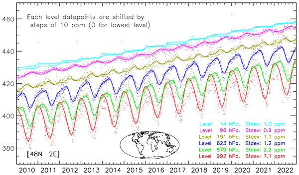
Figure 2 shows the time series of CAMS modelled atmospheric concentrations and the climatological fit using Eq. (2). The figure illustrates the growth rate that is identical at each level of the atmosphere, and the annual cycle that is much more pronounced in the low atmospheric layers than at higher altitudes. The seasonal cycle takes different shapes depending on the atmospheric layers, and it appears that two harmonics are sufficient to describe these shapes. Figure 2 is for one location, that is chosen here because it is at the centre of the AirCore samples described in Sect. 2.3 (see Fig. 1), but similar conclusions can be drawn from the results at other locations, although the seasonal cycle amplitude is much less in the southern hemisphere (see Fig. 5).

Figure 2Time series of the CAMS modelled concentrations at various atmospheric levels in the atmosphere (dots) and best fit adjustment (lines) using analytical Eq. (1). The RMS errors for the fit are provided at the lower-right of the figure. This is for the location [48° N 2° E] which is at the center of the AirCore samples described in Sect. 2.3. The datapoints and fit for each level have been shifted by 10 ppm to avoid overlap (no shift for the lowest level).
As expected, there is some scatter around the climatological fit. This scatter is linked to inter-annual as well as synoptic variability. For this particular location, it is on the order of 1 ppm in the mid and high atmosphere (above 700 hPa) but higher in the low atmospheric layers, in direct interaction with CO2 fluxes at the surface. The misfit is a quantification of the variability of atmospheric CO2 concentrations that cannot be described by the climatology. In the following, we evaluate both the CAMS modelling and its climatologic fit against independent measurements. Note that neither the AirCore profiles nor the TCCON measurements have been used to constrain the CAMS modelling. They are therefore truly independent from the modelled data.
3.2 Evaluation against AirCore profiles
We first use the 80 AirCore profiles described in Sect. 2.3 to evaluate both the CAMS modelling and its climatological fit. The model vertical sampling uses hybrid sigma coordinates that vary with the surface pressures. All model-AirCore comparisons are done at the hybrid sigma levels and we account for the surface pressure variations to sample the AirCore profiles at the corresponding model layers. The results are shown for a standard surface pressure of 1013 hPa.
Over France (Fig. 3), the biases are very similar for the model and its climatological fit, as expected. They are less than 0.5 ppm for the mid atmosphere but are significantly larger (1–2 ppm) both in the high atmosphere (above 200 hPa) and in the low atmosphere (below 850 hPa). The standard deviation (SD) of the model is less than 1 ppm in the middle atmosphere (between 300 and 800 hPa) but takes large values (≈ 2 ppm) in the mixing layer. The standard deviation of the climatological fit is close to 1.5 ppm within the free troposphere, and takes large values in the low atmosphere, consistent with that of the CAMS product.
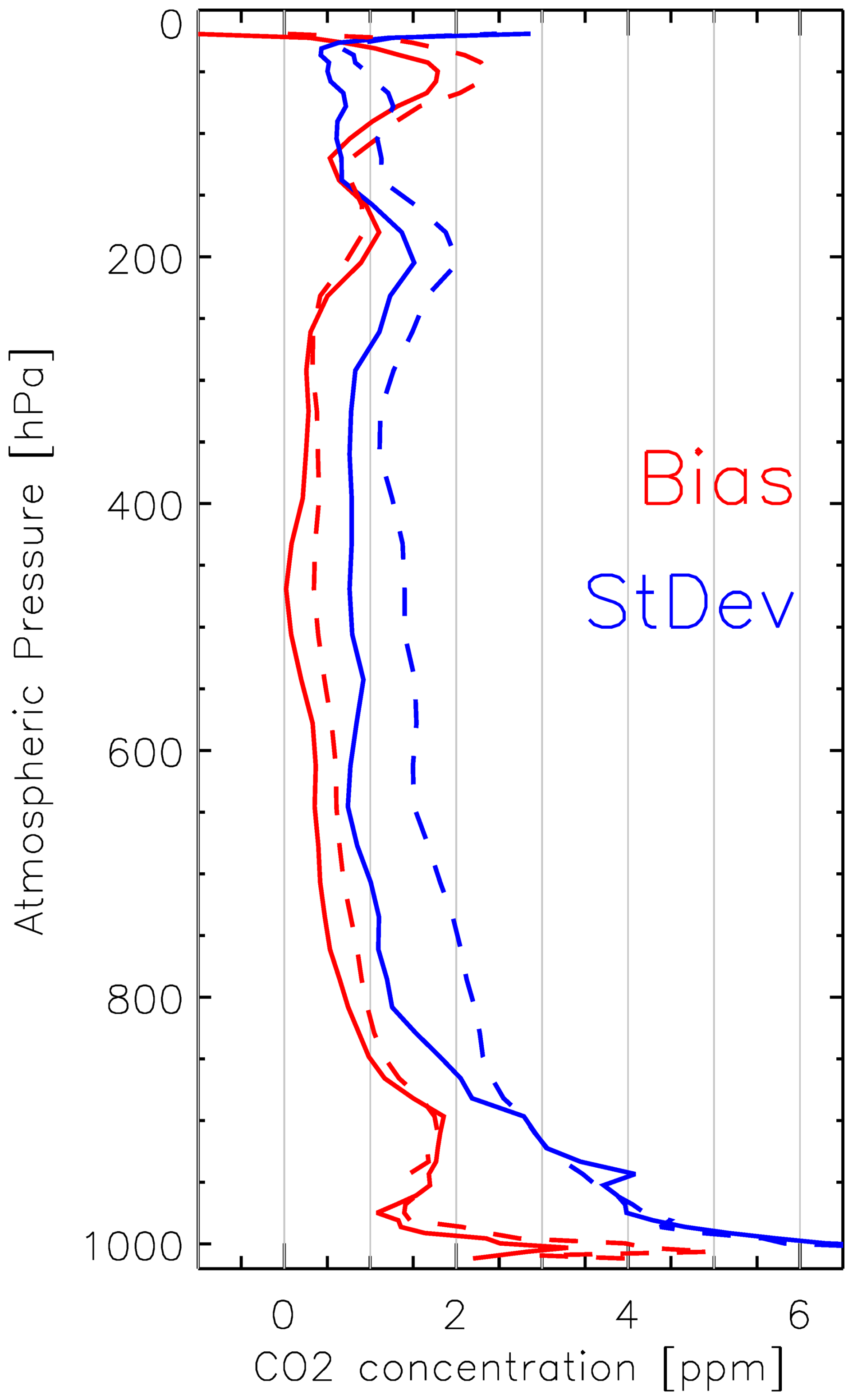
Figure 3Statistical comparison (Red: Biases; Blue: Standard deviation) of the AirCore vertical samples against both the CAMS modelling (plain lines) and its climatological fit (dashed lines).
The larger SD values of the climatological fit than the model are expected as the former cannot reproduce neither the inter-annual anomalies nor the synoptic variability. Nevertheless, the 2 ppm standard deviation is much less than both the growth over the analysis period and the amplitude of the seasonal cycle, which confirms that the climatological fit reproduces most of the CO2 concentration variability. In addition, the standard error of the climatological fit is larger, but on the same order of magnitude as the typical difference between the CAMS modelling and its climatological fit.
We acknowledge, however, that the statistics reported here may not be representative of the globe as a whole. On the one hand, synoptic variability, which cannot be captured by the climatological fit, is larger at mid-latitudes than in tropical regions. On the other hand, the high density of CO2 monitoring stations in Western Europe provides strong observational constraints on the CAMS modelling that are not available in all regions. Further evaluation against a more geographically distributed set of measurements is therefore necessary. To this end, we use a more diverse dataset of AirCore profiles acquired and made available by NOAA (Baier et al., 2023).
The dataset describes 145 profiles of atmospheric composition. More than half (84) of these profiles were acquired in the vicinity of Boulder, Colorado. Note that the surface pressure at Boulder is around 800 hPa, whereas Fig. 4 is shown as a function of equivalent pressure based on the hybrid sigma levels. At this site, the bias is very small for most of the troposphere and increases to around 2 ppm in the stratosphere, which is consistent with the results of the French site. The standard deviation is around 1 ppm in the free troposphere and stratosphere, and increases to ≈ 2 ppm in the mixing layer, again consistently with the results presented above. Lamont, with 32 AirCore samples, shows a very high standard deviation in the low atmosphere. A deeper analysis shows that this is due to 10 samples acquired between 22 July and 27 July 2018 when the concentration (observed and modelled by CAMS) differed strongly from the climatology. Other sites have too few samples for a meaningful statistical analysis but the comparisons are consistent with a modelling error on the order of 2 ppm. The error appears to be on the order of a few ppm, and larger in the low atmosphere.

Figure 4Statistical comparison of the NOAA AirCore vertical samples (Baier et al., 2023) against the climatological fit of the CAMS modelling. The statistical estimates are made for a number of locations where the profiles have been acquired. The figure indicates in parentheses the number of available profiles to compute the statistics. Left figure shows the biases whereas the right figure is for the Standard Deviation.
Overall, the analysis of the NOAA dataset indicates that the statistical results obtained at the French site, for which a large number of profiles are available, are broadly representative of those obtained in other regions where AirCore profiles are available.
3.3 Evaluation against TCCON
TCCON stations are distributed over the globe, which provides some indication of the spatial variability of the model performance. However, the TCCON standard products only provide a total column estimate with no indication on the vertical distribution. We therefore evaluate the total CO2 column concentration from the CAMS modelling as well as its climatological fit as in Eq. (3). The column is computed with a constant vertical weighting without accounting for the vertical sensitivity of the remote sensing product (the TCCON product is a best estimate of the total column and is therefore relevant for our evaluation). We also evaluate the CAMS and climatological vertical profiles: we compute a weighted total column using the prior and the AK provided with the TCCON retrieval datasets.
The results shown in Fig. 5 confirm the spatial variability of the statistics with smaller errors in the southern hemisphere and in the tropics than in the mid and high latitudes of the Northern hemisphere. The errors are on the order of 1 ppm. As expected, the errors are larger for the climatological fit than they are for the CAMS modelling, with three exceptions (Hefei, Manaus and Darwin) where they are almost identical. The results when using the unweighted and weighted total columns are very similar (see Fig. 5) indicating that the noise introduced by the vertical sensitivity is small in comparison to other sources of uncertainty.

Figure 5Statistical comparison (Standard deviation) of the TCCON total column against estimates from the CAMS modelling (green), the climatological fit (blue) and the GGG2020 prior used for the TCCON retrieval (red). The stations are sorted according to their latitude. For each station, the top bar shows the comparison of XCO2 without accounting for the averaging kernels (AK); the bottom bar is derived from the full vertical profile (either CAMS or Clim) and uses the AK for the total column estimate. This figure uses the datasets described in Notholt et al. (2026), Morino et al. (2022a, b, c), Deutscher et al. (2023a, b), Wunch et al. (2022), Strong et al. (2022), Dubey et al. (2022a, b), Sussmann et al. (2025), Liu et al. (2023), Weidmann et al. (2023), Iraci et al. (2022), García et al. (2022), Shiomi et al. (2022), Hase et al. (2024), Sherlock et al. (2022), Petri et al. (2024), Buschmann et al. (2022), Wennberg et al. (2025), Warneke et al. (2024), Wennberg et al. (2022), Té et al. (2022), De Mazière et al. (2022), Kivi et al. (2026), Zhou et al. (2022).
Note that the prior used for the TCCON estimate (Laughner et al., 2023) shows a difference with respect to the posterior value that is significantly larger than that obtained with the climatological fit. This strongly indicates that this fit could offer a better prior for TCCON estimates. However, the TCCON posterior value is loosely constrained by its prior, so that the use of a better prior may not change significantly the TCCON XCO2 estimates. For TCCON retrievals of the total column, the prior information of importance is the vertical profile and the fidelity of the prior in the higher atmospheric levels that are less constrained by measurements. Thus, although the climatology described in this paper appears closer to the “truth” than the GGG2020 prior, there is no demonstration that its use would result in a better posterior estimate of the column from TCCON measurements. Our analysis does show, nevertheless, that our climatology is accurate within ≈ 1 ppm, with spatial variations, and in particular a North-South gradient.
3.4 Amplitude of the seasonal cycle
Figure 6 shows the amplitude of the CO2 seasonal cycle at various levels in the atmosphere along longitude 25° E, chosen to maximize the coverage of land surfaces. The amplitude of the cycle is computed directly from the four Ai coefficients (A1 to A4) of Eq. (2). As expected, the seasonal cycle amplitude is larger in the lower atmospheric layers than it is higher up. The seasonal cycle also varies strongly with latitude: It is less than 2 ppm south of 30° S but takes values of more than 10 ppm north of 10° N, a difference which is a direct consequence of the fraction of land surfaces at the mid and high latitudes of the two hemispheres. Note that the seasonal cycle is rather high over the Sahara Desert (15–30° N) despite the absence of vegetation. It results from the transport of CO2 from other regions of the northern hemisphere with vegetation cover that drives a large seasonal cycle of the CO2 fluxes. In the high atmosphere, the seasonal cycle amplitude is smaller than in the low atmospheric levels but remains significant, up to 5 ppm. The seasonal cycle in the high atmosphere is not necessarily in phase with that observed at lower atmospheric levels, as for instance shown in Fig. 2.

Figure 6Amplitude of the CO2 seasonal cycle at various atmospheric levels as a function of latitude along the 25° E meridian.
Figure 7 shows a global map of the amplitude of the XCO2 seasonal cycle. The range of variation is large with values less than 2 ppm in most of the Southern hemisphere (with some exceptions over South America, Africa and Northern Australia) and up to 12 ppm over Siberia. The structure is mostly zonal, with a strong South-North gradient, although larger values are observed over the eastern part of the continents (with respect to the western part) at the northern mid and high latitudes. Regions of high elevation also show a reduced seasonal cycle of CO2 with respect to other regions of the same latitude.

Figure 7Amplitude of the XCO2 seasonal cycle.
3.5 Error of the Fit
Figure 2 shows time series of CAMS simulations together with the climatological fit at various levels in the atmosphere for a specific location chosen at the centre of the AirCore landings of Fig. 1. A similar analysis (not shown) can be performed over the XCO2 time series as in Eq. (3). Figure 8 shows the RMS deviation of the XCO2 fit as a function of location. Typical values are between 0.5 and 1.6 ppm with the smallest values observed in the Pacific, close to Hawaii and the Mauna Loa observatory, and the largest value over northeast China. Over the northern hemisphere, the deviation of the fit is much smaller than the seasonal cycle amplitude (Fig. 7) indicating that the seasonal cycle is fairly constant from year to year, which is a main hypothesis of the climatological fit developed in this paper. The deviation of the fit is less than 1 ppm over most of the oceans but takes larger values over the continents of the Northern hemisphere where vegetation fluxes, together with synoptic variability in the atmospheric transport, lead to day-to-day variations (Fig. 2) that cannot be reproduced by the climatology.

Figure 8RMS difference [ppm] between the XCO2 CAMS simulation and the climatological fit. The symbols overlaid on the map are at the location of the TCCON stations and indicate the error of the climatological fit with respect to the TCCON measurement, as in Fig. 5.
Overlaid on Fig. 8 are the standard deviations of the differences between the climatological analysis and the TCCON retrievals. In general, the typical differences with TCCON are slightly larger (a few tenths of a ppm) than the differences with CAMS but the spatial structure is consistent with the largest and smallest values found in the same areas. This consistency indicates that the deviation from the fit is a good indicator for the statistical error of the XCO2 concentration as described by the climatological product.
3.6 Vertical Covariance
We now analyze the vertical covariance of the climatological fit errors. One approach is to use the AirCore profiles described in Sect. 2.3 and analyzed in Sect. 3.2. There are about 80 profiles available in the vicinities of both Trainou (France) and Boulder (CO) locations, which is sufficient for a statistical analysis. The differences between the AirCore profiles and the climatological fit are computed at the model level resolution and used to compute variance-covariances and vertical correlations, which are shown in Fig. 9 for the Trainou site and in Fig. S1 (in the Supplement) for Boulder. The number of profiles is insufficient at the other sites for a meaningful statistical evaluation. Note that we also attempted an analysis for each of the 4 meteorological seasons at the Boulder and Trainou sites, but the sample is then insufficient to draw firm conclusions.

Figure 9Variance-covariance (left) and correlation matrices of the CO2 concentration deviations. The first row is based on the difference between the CAMS simulations and the climatological fit. The second row is based on the difference between the AirCore profiles and the climatological fit. The figures on the left show the square root of the covariance (bound at zero), expressed in ppm while the figures on the right show the correlation of the deviations. A similar figure for the Boulder site is shown in the Supplement.
The other approach is to use the CAMS simulation as the truth, compute the difference with the climatological fit at each time step and atmospheric level, and then compute a vertical variance-covariance from the time series of the differences. This shall be done independently for each of the model grid cells. In Fig. 9, we show the result for the model grid cell [48° N; 2° E] at the center of the French AirCore samples (Fig. 1), but similar analyses can be produced over all grid cells.
As expected, there is some vertical correlation on the errors (both in the model and in the AirCore samples) which leads to positive correlation and covariances. Some weak negative correlations are observed between the stratosphere and the troposphere. The two methods lead to rather similar results. The variances and covariances have the same order of magnitude, with larger values in the low atmosphere. There is a local maximum on the covariance around ≈ 150 hPa which corresponds to the troposphere-stratosphere transition, whose height may vary with a temporality that is poorly reproduced by the modelling. The vertical correlation estimates are rather similar, although slightly larger when computed against the model than against the AirCores. Overall, for this particular location, it appears that the error variance-covariance of the climatological fit, evaluated against the in-situ measurements, can be approximated by the value derived from the CAMS analysis.
Similar conclusions can be derived for the Boulder location (Fig. S1). The surface is much higher (≈ 1600 m) with an atmospheric pressure around 800 hPa. The variances and covariances are smaller than they are at the French site, both for the modelling approach and for the AirCore evaluation. The two approaches show very similar patterns, although the correlations are slightly larger (vertically extended) in the modelling analysis than when using the AirCore measurements.
4.1 Physical interpretation
The results demonstrate that a large fraction of the atmospheric CO2 variability can be represented by the combination of (i) the growth rate measured at the iconic Mauna Loa station and (ii) a stationary seasonal cycle described by two harmonics. This confirms that, at first order, the temporal evolution of atmospheric CO2 is dominated by large-scale processes that are spatially coherent: the anthropogenic trend and the biospheric seasonal exchange.
The success of the approach reflects two key properties of atmospheric CO2:
-
Rapid large-scale mixing, which ensures that the long-term growth rate is nearly uniform across latitudes and vertical levels.
-
Strong periodicity of biospheric fluxes, particularly in the Northern Hemisphere, which produces a remarkably regular seasonal cycle whose shape is well captured by annual and semi-annual harmonics.
The fact that the residual variability is typically below 1–2 ppm in the free troposphere indicates that interannual changes in fluxes and synoptic transport, while detectable, remain second-order compared to the seasonal amplitude of the concentration (up to 10–12 ppm at northern mid-latitudes).
However, the degradation of performance in the planetary boundary layer highlights the intrinsic limitation of any climatological approach: surface flux variability and boundary-layer dynamics introduce short-term fluctuations that cannot be captured by stationary harmonics.
4.2 Relation to previous empirical background models
The approach developed here has similarities with empirical background models such as those proposed by Reuter et al. (2012) and Laughner et al. (2023), which describe atmospheric CO2 using a simple analytical formulation and a reference to the Mauna Loa and American Samoa observations for the latter. Our approach is slightly more complex, however. Indeed, Reuter et al. (2012) used only 17 coefficients to describe the CO2 variability over the full Earth and atmospheric levels, while the approach of Laughner et al. (2023) is purely analytical with a set of empirical values embedded within the equations. Our approach uses only 5 coefficients, but these are different for each grid point and atmospheric level. Thus, while the two former approaches are purely analytical and can be implemented as a simple analytical function, our approach requires a 25 MB dataset as input. We have compared the performance of these approaches. Although the fully analytical functions do reproduce the main variations of atmospheric CO2, their performance appears limited compared to our approach. Reuter et al. (2012) assumed a constant growth rate in the atmosphere while the true growth has accelerated in the past decade. This is corrected in the method of Laughner et al. (2023) that uses observations to constrain the mean trend, but the evaluation against TCCON shows that our approach leads to significantly lower errors. Besides, Laughner et al. (2023) assumed no variation of the concentrations along the longitudes, which is a strong limitation, in particular for the low atmospheric levels.
The analytical approach of Reuter et al. (2012) or Laughner et al. (2023) may be sufficient when only a rough estimate of the CO2 profile is needed. Our approach brings additional accuracy at the cost of some complexity.
The SLIMCO2 approach presented in Appendix A of Noël et al. (2022) has many similarities with that proposed here. Both use more than 10 years of a global 4D description of atmospheric CO2 (CarbonTracker for SLIMCO2, CAMS for our product). The main difference is our use of an analytical function versus the explicit estimate of the detrended concentration at 36 time steps within the year. Another difference is the way the growth rate is modelled, based on the Mauna Loa time series in our approach, and assuming a linear growth between the global mean value derived from the atmospheric transport simulation on 1 January in SLIMCO2. Through direct contact (Maximilian Reuter, personal communication, 2026), we compared the XCO2 estimates of the two approaches over a number of selected targets. The temporal profiles of XCO2 generated by the two methods are very similar (trends and seasonal cycles) although not identical. There are some differences in the overall trend and the seasonal cycle described by our method is smoother. The statistical difference is on the order of 0.30 ppm and varies spatially with a maximum of 0.47 ppm among the targets we analysed. Overall, the differences are significantly smaller than the likely differences between the modelled value and the truth. The differences result from the variations in the two approaches. There is no strong argument for using one versus the other.
4.3 Implications for satellite retrievals
Our simple modelling of the atmospheric CO2 could be used as an accurate prior for satellite retrievals of the atmospheric concentration. Indeed, the validation against both AirCore measurements and TCCON stations has shown an accuracy better than 1.5 ppm on XCO2, and a reasonable description of the vertical profile. This suggests that the proposed formulation could serve as a physically informed prior for column or profile retrievals. Because the formulation is linear in its parameters, it can be easily implemented and can also be updated as new Mauna Loa data become available. Besides, as the de-seasonalized growth rate does not vary strongly from month to month, the Mauna Loa time series can be extrapolated in time over a few months with no significant added error on the climatological product.
Importantly, the vertical covariance analysis indicates that errors of the climatological fit are vertically correlated, especially within the troposphere. This has consequences for the specification of background error covariance matrices in inversion systems. The similarity between covariance structures derived from CAMS and from AirCore comparisons suggests that the model-based estimate provides a reasonable approximation of real atmospheric variability. Thus, the covariance matrices, which have been derived based on the CAMS vs analytical fit differences, may be used for the satellite-based inversions of the CO2 profiles.
4.4 Potential for satellite retrieval validation
The proposed climatological product may also provide a useful framework for a first evaluation of space-borne CO2 retrievals. Because it captures the dominant components of atmospheric variability – namely the long-term trend and the stationary seasonal cycle – it defines a physically consistent baseline against which satellite products can be evaluated. Obviously, the satellite products aim at improving our knowledge of atmospheric concentration, and are therefore designed to achieve an accuracy that is higher than that of the climatological product. Yet, a comparison of the retrievals against this climatology may be used as a first validity check during the commissioning phase.
In regions where the residual variability relative to the climatology is small (e.g. remote oceanic areas, tropical regions, or the Southern Hemisphere), the atmospheric state is largely controlled by well-mixed background conditions. In such regions, discrepancies between satellite retrievals and the climatological estimate are more likely to reflect retrieval biases, instrumental effects, or forward-model errors rather than unresolved atmospheric variability. These areas therefore offer favorable conditions for assessing systematic errors and long-term stability.
Conversely, in regions where the residual variability is large – in particular over continental mid- and high latitudes of the Northern Hemisphere – synoptic transport, boundary-layer dynamics, and heterogeneous surface fluxes introduce short-term fluctuations that are not captured by the climatological representation. In these areas, differences between satellite products and the climatological estimate cannot be interpreted solely as retrieval errors, since part of the discrepancy may arise from real atmospheric variability. The spatial structure of the fit residuals thus provides an objective indicator of where satellite validation can rely on a stable background and where additional caution is required.
More generally, the product may help separate two components of satellite error diagnostics: (i) systematic biases relative to a well-characterized background, and (ii) representation errors linked to unresolved atmospheric variability. This distinction is particularly relevant for the evaluation of high-precision missions targeting sub-ppm accuracy.
4.5 Limitations of the approach, and potential for improvements
Several limitations of the approach must be acknowledged, and offer opportunities for improvements.
Our approach uses the measurements at Mauna Loa to describe the mean growth rate at all points over the globe. We made this choice because the Mauna Loa time series is easily accessible, continuous, regularly updated and available over a long time period. The near-uniform growth rate observed across latitudes and vertical levels is consistent with characteristic tropospheric mixing times of a few weeks zonally, a few months meridionally within a hemisphere, and approximately 1 year between hemispheres (Jacob et al., 1997). The 1-year time scale for inter-hemispheric exchange suggests the use of a different growth rate for the Northern and Southern hemispheres. Thus, over the southern hemisphere, one could replace the Mauna Loa time series by that from American Samoa, operated by NOAA-GML (Thoning et al., 2025) or the observations from Amsterdam Island operated by LSCE, two locations in the Southern Hemisphere that sample “background” concentrations. We compared the smoothed de-seasonalized time series of Mauna-Loa and American Samoa. There is a bias of ≈ 2.5 ppm, with higher concentrations at Mauna Loa, due to the time required for anthropogenic CO2 emissions, which occur predominantly in the Northern Hemisphere, to be transported to the Southern Hemisphere. The bias is increasing with time as a result of increasing emissions. We used the American Samoa time series, instead of Mauna Loa, to quantify the trend and redid the evaluation against TCCON. There is no significant improvement, nor degradation, of the consistency with TCCON CO2 column estimates, although we expected some differences between Northern and Southern Hemisphere stations.
The method assumes that the seasonal cycle does not change significantly over the analysis period. Yet, observations of surface concentrations of CO2 over several decades indicate an increase in the amplitude of the seasonal cycle in the Northern hemisphere (Graven et al., 2013; Piao et al., 2018). Our approximation appears valid over 13 years, but long-term changes in biospheric phenology exacerbated by climate change could eventually invalidate this assumption. A new fit against updated time series may therefore become necessary in the future to account for these changes.
Our approach shows large errors in the lower atmospheric layers where surface fluxes and mixing heights vary rapidly. A purely harmonic representation cannot reproduce synoptic variability, frontal passages, or localized flux events. This is inherent to the climatological approach.
We have validated the CAMS and climatological fit against AirCore over a single region which may not be representative of the whole globe. This region (central France) shows a large seasonal cycle and synoptic variability, when compared to other regions of the globe, as shown in Figs. 6 and 7. Yet, other regions (such as Siberia and Eastern Asia) show even larger cycle amplitudes and variability which may be difficult to handle by our simple approach. In addition, the CAMS modelling over western Europe is well constrained by a high density of surface observations that is not available elsewhere. One may therefore question the representativeness of some results. Figure 4 shows some additional comparisons using the AirCore from NOAA (Baier et al., 2023), that are consistent with the results of the France samples, but most have been acquired over the United States which is also well constrained by the surface observations. Further validation using airborne measurements over more diverse areas could provide additional evaluation.
In this paper, we have developed and evaluated a climatological representation of atmospheric CO2 variability at seasonal and interannual scales based on a multi-year 4D reanalysis. This representation is available in near-real time thanks to the near real time availability of the CO2 measurements at the Mauna Loa station, operated by the Scripps Institution of Oceanography and NOAA. The analysis confirms that, at first order, atmospheric CO2 variability is dominated by a globally coherent growth rate and a largely stationary seasonal cycle driven by biospheric fluxes. The seasonal component can be robustly represented using only two harmonics, showing that most of the observed variability can be described with a limited number of parameters.
Evaluation against independent AirCore vertical profiles and TCCON column retrievals demonstrates that the typical representation error of the climatological fit is on the order of 1–1.5 ppm for XCO2, with smaller errors over the Southern Hemisphere and oceanic regions, and larger residuals over northern continental areas. These results confirm that a substantial fraction of atmospheric CO2 variability is highly regular in space and time.
The residual deviations from the climatology, typically around 1 ppm and regionally up to 1.5 ppm, define the scale of atmospheric variability that cannot be captured by a stationary representation. This provides a physically based benchmark for assessing the accuracy requirements of satellite retrievals and highlights the level of systematic precision needed for applications in atmospheric inversions.
Beyond its analytical interest, the climatological product offers a compact and practical framework for representing atmospheric CO2 fields and their associated error structures. By separating the dominant climatological signal from higher-frequency variability, it may facilitate the evaluation of satellite observations, the specification of prior information in retrieval algorithms, and the interpretation of regional CO2 anomalies. The climatological product may also be used for other purposes when an estimate of the CO2 concentration is needed, in particular in near-real-time. For instance, it is used among other predictors by the Copernicus Marine Environment Service (https://marine.copernicus.eu/, last access: 12 November 2026) to estimate the surface ocean fugacity and air-sea fluxes about one month behind real time (Chau et al., 2024).
The use of the climatological product relies on a dataset (netCDF file) that provides the 5 parameters on a latitude-longitude grid and for 79 atmospheric levels. The file is 25 MB. In addition, the analysis led to variance-covariance matrices for each of the model grid points. The corresponding file will be used as prior information for the derivation of CO2 profiles based on the MicroCarb satellite measurements. The file is 400 MB and is available for other uses (see Data availability below).
Two NetCDF files have been created in the context of this study and are available for any use. The first one contains the 5 Ai coefficients in Eq. (2) on a lat-lon-pressure grid. The second one contains the vertical variance-covariance matrices (Figs. 9 and S1) on a lat-lon grid. They are available on request from the corresponding author or at the following links: https://sharebox.lsce.ipsl.fr/index.php/s/xGCD36KuYmN3OcZ (last access: 12 November 2026) and https://sharebox.lsce.ipsl.fr/index.php/s/dT5etwySTrWgIBN (last access: 12 November 2026). The TCCON data is available from https://doi.org/10.14291/TCCON.GGG2020 (Wunch et al., 2020). The LSCE Aircore data is available from https://doi.org/10.25326/787 (Ramonet et al., 2025). The NOAA Aircore data is available from https://doi.org/10.15138/6AV0-MY81 (Baier et al., 2021).
The supplement related to this article is available online at https://doi.org/10.5194/acp-26-16247-2026-supplement.
FMB created the priors code, carried out the validation, and led the writing of the manuscript. FC developed the CAMS modelling that is used in the paper. MR developed the French AirCore program that is used, together with the NOAA samples and TCCON retrievals, for the product evaluation. FMB prepared the manuscript with contributions from all co-authors.
The contact author has declared that none of the authors has any competing interests.
Publisher's note: Copernicus Publications remains neutral with regard to jurisdictional claims made in the text, published maps, institutional affiliations, or any other geographical representation in this paper. The authors bear the ultimate responsibility for providing appropriate place names. Views expressed in the text are those of the authors and do not necessarily reflect the views of the publisher.
The authors are grateful to the teams and funding bodies that make possible the measurements from the TCCON network (https://doi.org/10.14291/TCCON.GGG2020, Wunch et al., 2020) as well as the AirCore profiles (https://doi.org/10.15138/6AV0-MY81, Baier et al., 2021, 2023) that have been used for evaluation in this paper.
This paper was edited by Jason West and reviewed by three anonymous referees.
Baier, B., Sweeney, C., Newberger, T., Higgs, J., Wolter, S., Tans, P. P., and NOAA Global Monitoring Laboratory: NOAA AirCore atmospheric sampling system profiles (Version 20260717), NOAA GML [data set], https://doi.org/10.15138/6AV0-MY81, 2021.
Baier, B. C., Sweeney, C., and Chen, H.: Chapter 8 – The AirCore atmospheric sampling system, in: Field Measurements for Passive Environmental Remote Sensing, edited by: Nalli, N. R., Elsevier, 139–156, https://doi.org/10.1016/B978-0-12-823953-7.00014-9, 2023.
Buschmann, M., Petri, C., Palm, M., Warneke, T., and Notholt, J.: TCCON data from Ny-Ålesund, Svalbard (NO), Release GGG2020.R0 (Version R0), CaltechDATA [data set], https://doi.org/10.14291/TCCON.GGG2020.NYALESUND01.R0, 2022.
Chau, T.-T.-T., Chevallier, F., and Gehlen, M.: Global analysis of surface ocean CO2 fugacity and air-sea fluxes with low latency, Geophys. Res. Lett., 51, e2023GL106670, https://doi.org/10.1029/2023GL106670, 2024.
Chevallier, F., Ciais, P., Conway, T. J., Aalto, T., Anderson, B. E., Bousquet, P., Brunke, E. G., Ciattaglia, L., Esaki, Y., Fröhlich, M., Gomez, A. J., Gomez-Pelaez, A. J., Haszpra, L., Krummel, P., Langenfelds, R., Leuenberger, M., Machida, T., Maignan, F., Matsueda, H., Morguí, J. A., Mukai, H., Nakazawa, T., Peylin, P., Ramonet, M., Rivier, L., Sawa, Y., Schmidt, M., Steele, P., Vay, S. A., Vermeulen, A. T., Wofsy, S., and Worthy, D.: CO2 surface fluxes at grid point scale estimated from a global 21-year reanalysis of atmospheric measurements, J. Geophys. Res., 115, D21307, https://doi.org/10.1029/2010JD013887, 2010.
Chevallier, F., Lloret, Z., Cozic, A., Takache, S., and Remaud, M.: Toward high-resolution global atmospheric inverse modelling using graphics accelerators, Geophys. Res. Lett., 50, https://doi.org/10.1029/2022GL102135, 2023.
Ciais, P., Rayner, P., Chevallier, F., Bousquet, P., Logan, M., Peylin, P., and Ramonet, M.: Atmospheric inversions for estimating CO2 fluxes: methods and perspectives, Climatic Change, 103, 69–92, https://doi.org/10.1007/s10584-010-9909-3, 2010.
Crisp, D., Atlas, R. M., Breon, F.-M., Brown, L. R., Burrows, J. P., Ciais, P., Connor, B. J., Doney, S. C., Fung, I. Y., Jacob, D. J., Miller, C. E., O’Brien, D., Pawson, S., Randerson, J. T., Rayner, P., Salawitch, R. J., Sander, S. P., Sen, B., Stephens, G. L., Tans, P. P., Toon, G. C., Wennberg, P. O., Wofsy, S. C., Yung, Y. L., Kuang, Z., Chudasama, B., Sprague, G., Weiss, B., Pollock, R., Kenyon, D., and Schroll, S.: The Orbiting Carbon Observatory (OCO) mission, Adv. Space Res., 34, https://doi.org/10.1016/j.asr.2003.08.062, 2004.
De Mazière, M., Sha, M. K., Desmet, F., Hermans, C., Scolas, F., Kumps, N., Zhou, M., Metzger, J.-M., Duflot, V., and Cammas, J.-P.: TCCON data from Réunion Island (RE), Release GGG2020.R0 (Version R0), CaltechDATA [data set], https://doi.org/10.14291/TCCON.GGG2020.REUNION01.R0, 2022.
Deutscher, N. M., Griffith, D. W. T., Paton-Walsh, C., Jones, N. B., Velazco, V. A., Wilson, S. R., Macatangay, R. C., Kettlewell, G. C., Buchholz, R. R., Riggenbach, M. O., Bukosa, B., John, S. S., Walker, B. T., and Nawaz, H.: TCCON data from Wollongong (AU), Release GGG2020.R0 (Version R0), CaltechDATA [data set], https://doi.org/10.14291/TCCON.GGG2020.WOLLONGONG01.R0, 2023a.
Deutscher, N. M., Griffith, D. W. T., Paton-Walsh, C., Velazco, V. A., Wennberg, P. O., Blavier, J.-F., Washenfelder, R. A., Yavin, Y., Keppel-Aleks, G., Toon, G. C., Jones, N. B., Kettlewell, G. C., Connor, B. J., Macatangay, R. C., Wunch, D., Roehl, C., and Bryant, G. W.: TCCON data from Darwin (AU), Release GGG2020.R0 (Version R0), CaltechDATA [data set], https://doi.org/10.14291/TCCON.GGG2020.DARWIN01.R0, 2023b.
Dubey, M., Lindenmaier, R., Henderson, B. G., Allen, N. T., Roehl, C. M., Blavier, J.-F., Love, S., and Wunch, D.: TCCON data from Four Corners (US), Release GGG2020.R0 (Version R0), CaltechDATA [data set], https://doi.org/10.14291/TCCON.GGG2020.FOURCORNERS01.R0, 2022a.
Dubey, M. K., Henderson, B. G., Allen, N. T., Blavier, J.-F., Roehl, C. M., and Wunch, D.: TCCON data from Manaus (BR), Release GGG2020.R0 (Version R0), CaltechDATA [data set], https://doi.org/10.14291/TCCON.GGG2020.MANAUS01.R0, 2022b.
Forkel, M., Carvalhais, N., Rödenbeck, C., Keeling, R., Heimann, M., Thonicke, K., Zaehle, S., and Reichstein, M.: Enhanced seasonal CO2 exchange caused by amplified plant productivity in northern ecosystems, Science, 351, 696–699, https://doi.org/10.1126/science.aac4971, 2016.
Franz, D., Acosta, M., Altimir, N., et al.: Towards long-term standardised carbon and greenhouse gas observations for monitoring Europe's terrestrial ecosystems: a review, Int. Agrophys., 32, 439–455, https://doi.org/10.1515/intag-2017-0039, 2018.
Friedlingstein, P., Le Quéré, C., O’Sullivan, M., Hauck, J., Landschützer, P., Luijkx, I. T., Li, H., van der Woude, A., Schwingshackl, C., Pongratz, J., Regnier, P., Andrew, R. M., Bakker, D. C. E., Canadell, J. G., Ciais, P., Gasser, T., Jones, M. W., Lan, X., Morgan, E., Olsen, A., Peters, G. P., Peters, W., Sitch, S., and Tian, H.: Emerging climate impact on carbon sinks in a consolidated carbon budget, Nature, 649, 98–103, https://doi.org/10.1038/s41586-025-09802-5, 2026.
García, O. E., Schneider, M., Herkommer, B., Gross, J., Hase, F., Blumenstock, T., and Sepúlveda, E.: TCCON data from Izana (ES), Release GGG2020.R1 (Version R1), CaltechDATA [data set], https://doi.org/10.14291/TCCON.GGG2020.IZANA01.R1, 2022.
Graven, H. D., Keeling, R. F., Piper, S. C., Patra, P. K., Stephens, B. B., Wofsy, S. C., Welp, L. R., Sweeney, C., Tans, P. P., Kelley, J. J., Daube, B. C., Kort, E. A., Santoni, G. W., and Bent, J. D.: Enhanced seasonal exchange of CO2 by northern ecosystems since 1960, Science, 341, 1085–1089, 2013.
Hase, F., Herkommer, B., Groß, J., Blumenstock, T., Kiel, M., and Dohe, S.: TCCON data from Karlsruhe (DE), Release GGG2020.R2 (Version R2), CaltechDATA [data set], https://doi.org/10.14291/TCCON.GGG2020.KARLSRUHE01.R2, 2024.
Iraci, L. T., Podolske, J. R., Hillyard, P. W., Roehl, C., Wennberg, P. O., Blavier, J.-F., Landeros, J., Allen, N., Wunch, D., Zavaleta, J., Quigley, E., Osterman, G. B., Barrow, E., and Barney, J.: TCCON data from Indianapolis (US), Release GGG2020.R1 (Version R1), CaltechDATA [data set], https://doi.org/10.14291/TCCON.GGG2020.INDIANAPOLIS01.R1, 2022.
Jacob, D. J., Prather, M. J., Rasch, P. J., Shia, R.-L., Balkanski, Y. J., Beagley, S. R., Bergmann, D. J., Blackshear, W. T., Brown, M., Chiba, M., Chipperfield, M. P., de Grandpré, J., Dignon, J., Feichter, J., Genthon, C., Grose, W. L., Kasibhatla, P. S., Köhler, I., Kritz, M. A., Law, K. S., Penner, J. E., Ramonet, M., Reeves, C. E., Rotman, D. A., Stockwell, D. Z., Van Velthoven, P. F. J., Verver, G. H., Wild, O., Yang, H., and Zimmermann, P.: Evaluation and intercomparison of global atmospheric transport models using 222Rn and other short-lived tracers, J. Geophys. Res.-Atmos., 102, 5953–5970. https://doi.org/10.1029/96JD02955, 1997.
Jacobson, A. R., Schuldt, K. N., Miller, J. B., et al.: CarbonTracker CT2019B, NOAA/GML [data set], https://doi.org/10.25925/20201008, 2020.
Karion, A., Sweeney, C., Tans, P., and Newberger, T.: AirCore: an innovative atmospheric sampling system, J. Atmos. Ocean. Technol., 27, 1839–1853, https://doi.org/10.1175/2010JTECHA1448.1, 2010.
Keeling, C. D., Bacastow, R. B., Bainbridge, A. E., Ekdahl Jr., C. A., Guenther, P. R., Waterman, L. S., and Chin, J. F. S.: Atmospheric carbon dioxide variations at Mauna Loa Observatory, Hawaii, Tellus, 28, 538–551, https://doi.org/10.1111/j.2153-3490.1976.tb00701.x, 1976.
Kivi, R., Heikkinen, P., and Kyrö, E.: TCCON data from Sodankylä (FI), Release GGG2020.R1 (Version R1), CaltechDATA [data set], https://doi.org/10.14291/TCCON.GGG2020.SODANKYLA01.R1, 2026.
Laughner, J. L., Roche, S., Kiel, M., Toon, G. C., Wunch, D., Baier, B. C., Biraud, S., Chen, H., Kivi, R., Laemmel, T., McKain, K., Quéhé, P.-Y., Rousogenous, C., Stephens, B. B., Walker, K., and Wennberg, P. O.: A new algorithm to generate a priori trace gas profiles for the GGG2020 retrieval algorithm, Atmos. Meas. Tech., 16, 1121–1146, https://doi.org/10.5194/amt-16-1121-2023, 2023.
Laughner, J. L., Toon, G. C., Mendonca, J., Petri, C., Roche, S., Wunch, D., Blavier, J.-F., Griffith, D. W. T., Heikkinen, P., Keeling, R. F., Kiel, M., Kivi, R., Roehl, C. M., Stephens, B. B., Baier, B. C., Chen, H., Choi, Y., Deutscher, N. M., DiGangi, J. P., Gross, J., Herkommer, B., Jeseck, P., Laemmel, T., Lan, X., McGee, E., McKain, K., Miller, J., Morino, I., Notholt, J., Ohyama, H., Pollard, D. F., Rettinger, M., Riris, H., Rousogenous, C., Sha, M. K., Shiomi, K., Strong, K., Sussmann, R., Té, Y., Velazco, V. A., Wofsy, S. C., Zhou, M., and Wennberg, P. O.: The Total Carbon Column Observing Network's GGG2020 data version, Earth Syst. Sci. Data, 16, 2197–2260, https://doi.org/10.5194/essd-16-2197-2024, 2024.
Liu, C., Wang, W., Sun, Y., and Shan, C.: TCCON data from Hefei (PRC), Release GGG2020.R1 (Version R1), CaltechDATA [data set], https://doi.org/10.14291/TCCON.GGG2020.HEFEI01.R1, 2023.
Masarie, K. A. and Tans, P. P.: Extension and integration of atmospheric carbon dioxide data into a globally consistent measurement record, J. Geophys. Res., 100, 11593–11610, https://doi.org/10.1029/95JD00859, 1995.
Membrive, O., Crevoisier, C., Sweeney, C., Danis, F., Hertzog, A., Engel, A., Bönisch, H., and Picon, L.: AirCore-HR: a high-resolution column sampling to enhance the vertical description of CH4 and CO2, Atmos. Meas. Tech., 10, 2163–2181, https://doi.org/10.5194/amt-10-2163-2017, 2017.
Morino, I., Velazco, V. A., Hori, A., Uchino, O., and Griffith, D. W. T.: TCCON data from Burgos, Ilocos Norte (PH), Release GGG2020.R0 (Version R0), CaltechDATA [data set], https://doi.org/10.14291/TCCON.GGG2020.BURGOS01.R0, 2022a.
Morino, I., Ohyama, H., Hori, A., and Ikegami, H.: TCCON data from Rikubetsu (JP), Release GGG2020.R0 (Version R0), CaltechDATA [data set], https://doi.org/10.14291/TCCON.GGG2020.RIKUBETSU01.R0, 2022b.
Morino, I., Ohyama, H., Hori, A., and Ikegami, H.: TCCON data from Tsukuba (JP), 125HR, Release GGG2020.R0 (Version R0), CaltechDATA [data set], https://doi.org/10.14291/TCCON.GGG2020.TSUKUBA02.R0, 2022c.
Noël, S., Reuter, M., Buchwitz, M., Borchardt, J., Hilker, M., Schneising, O., Bovensmann, H., Burrows, J. P., Di Noia, A., Parker, R. J., Suto, H., Yoshida, Y., Buschmann, M., Deutscher, N. M., Feist, D. G., Griffith, D. W. T., Hase, F., Kivi, R., Liu, C., Morino, I., Notholt, J., Oh, Y.-S., Ohyama, H., Petri, C., Pollard, D. F., Rettinger, M., Roehl, C., Rousogenous, C., Sha, M. K., Shiomi, K., Strong, K., Sussmann, R., Té, Y., Velazco, V. A., Vrekoussis, M., and Warneke, T.: Retrieval of greenhouse gases from GOSAT and GOSAT-2 using the FOCAL algorithm, Atmos. Meas. Tech., 15, 3401–3437, https://doi.org/10.5194/amt-15-3401-2022, 2022.
Notholt, J., Petri, C., Warneke, T., and Buschmann, M.: TCCON data from Bremen (DE), Release GGG2020.R1 (Version R1), CaltechDATA [data set], https://doi.org/10.14291/TCCON.GGG2020.BREMEN01.R1, 2026.
Petri, C., Vrekoussis, M., Rousogenous, C., Warneke, T., Sciare, J., and Notholt, J.: TCCON data from Nicosia (CY), Release GGG2020.R1 (Version R1), CaltechDATA [data set], https://doi.org/10.14291/TCCON.GGG2020.NICOSIA01.R1, 2024.
Piao, S., Liu, Z., Wang, Y., Ciais, P., Yao, Y., Peng, S., Chevallier, F., Friedlingstein, P., Janssens, I. A., Peñuelas, J., Sitch, S., and Wang, T.: On the causes of trends in the seasonal amplitude of atmospheric CO2, Glob. Change Biol., 24, 608–616, https://doi.org/10.1111/gcb.13909, 2018.
Ramonet, M., Lopez, M., Rigouleau, L.-J., Lopez, D., Pernin, J., Ponthieu, T., Guedj, A., and Crevoisier, C. : AirCore – L2 – TRN site, Aeris [data set], https://doi.org/10.25326/787, 2025.
Reuter, M., Buchwitz, M., Schneising, O., Hase, F., Heymann, J., Guerlet, S., Cogan, A. J., Bovensmann, H., and Burrows, J. P.: A simple empirical model estimating atmospheric CO2 background concentrations, Atmos. Meas. Tech., 5, 1349–1357, https://doi.org/10.5194/amt-5-1349-2012, 2012.
Sherlock, V., Connor, B., Robinson, J., Shiona, H., Smale, D., and Pollard, D. F.: TCCON data from Lauder (NZ), 120HR, Release GGG2020.R0 (Version R0), CaltechDATA [data set], https://doi.org/10.14291/TCCON.GGG2020.LAUDER01.R0, 2022.
Shiomi, K., Kawakami, S., Ohyama, H., Arai, K., Okumura, H., Ikegami, H., and Usami, M.: TCCON data from Saga (JP), Release GGG2020.R0 (Version R0), CaltechDATA [data set], https://doi.org/10.14291/TCCON.GGG2020.SAGA01.R0, 2022.
Strong, K., Roche, S., Franklin, J. E., Mendonca, J., Lutsch, E., Weaver, D., Fogal, P. F., Drummond, J. R., Batchelor, R., Lindenmaier, R., and McGee, E.: TCCON data from Eureka (CA), Release GGG2020.R0 (Version R0), CaltechDATA [data set], https://doi.org/10.14291/TCCON.GGG2020.EUREKA01.R0, 2022.
Sussmann, R., Rettinger, M., and Mostafavi Pak, N.: TCCON data from Garmisch (DE), Release GGG2020.R1 (Version R1), CaltechDATA [data set], https://doi.org/10.14291/TCCON.GGG2020.GARMISCH01.R1, 2025.
Té, Y., Jeseck, P., and Janssen, C.: TCCON data from Paris (FR), Release GGG2020.R0 (Version R0), CaltechDATA [data set], https://doi.org/10.14291/TCCON.GGG2020.PARIS01.R0, 2022.
Thoning, K. W., Tans, P. P., and Komhyr W. D.: Atmospheric carbon dioxide at Mauna Loa Observatory: 2. Analysis of the NOAA GMCC data, 1974–1985, J. Geophys. Res., 94, 8549–8565, https://doi.org/10.1029/JD094iD06p08549, 1989.
Thoning, K. W., Crotwell A. M., and Mund, J. W.: Atmospheric Carbon Dioxide Dry Air Mole Fractions from continuous measurements at Mauna Loa, Hawaii, Barrow, Alaska, American Samoa and South Pole, 1973–present. Version 2025-04-26, National Oceanic and Atmospheric Administration (NOAA), Global Monitoring Laboratory (GML), Boulder, Colorado, USA, https://doi.org/10.15138/yaf1-bk21, 2025.
Warneke, T., Petri, C., Notholt, J., and Buschmann, M.: TCCON data from Orléans (FR), Release GGG2020.R1 (Version R1), CaltechDATA [data set], https://doi.org/10.14291/TCCON.GGG2020.ORLEANS01.R1, 2024.
Weidmann, D., Brownsword, R., and Doniki, S.: TCCON data from Harwell, Oxfordshire (UK), Release GGG2020.R0 (Version R0), CaltechDATA [data set], https://doi.org/10.14291/TCCON.GGG2020.HARWELL01.R0, 2023.
Wennberg, P. O., Roehl, C. M., Wunch, D., Toon, G. C., Blavier, J.-F., Washenfelder, R., Keppel-Aleks, G., and Allen, N. T.: TCCON data from Park Falls (US), Release GGG2020.R1 (Version R1), CaltechDATA [data set], https://doi.org/10.14291/TCCON.GGG2020.PARKFALLS01.R1, 2022.
Wennberg, P. O., Wunch, D., Roehl, C. M., Blavier, J.-F., Toon, G. C., and Allen, N. T.: TCCON data from Lamont (US), Release GGG2020.R1 (Version R1), CaltechDATA [data set], https://doi.org/10.14291/TCCON.GGG2020.LAMONT01.R1, 2025.
Wunch, D., Toon, G. C., Blavier, J. F. L., Washenfelder, R. A., Notholt, J., Connor, B. J., Griffith, D. W. T., Sherlock, V., and Wennberg, P. O.: The Total Carbon Column Observing Network, Philos. Trans. A Math. Phys. Eng. Sci., 369, 2087–2112, https://doi.org/10.1098/rsta.2010.0240, 2011.
Wunch, D., Wennberg, P. O., Griffith, D. W. T., Deutscher, N. M., Feist, D. G., Notholt, J., and Laughner, J. L.: 2020 TCCON Data Release (Version GGG2020), CaltechDATA [data set], https://doi.org/10.14291/TCCON.GGG2020, 2020.
Wunch, D., Mendonca, J., Colebatch, O., Allen, N. T., Blavier, J.-F., Kunz, K., Roche, S., Hedelius, J., Neufeld, G., Springett, S., Worthy, D., Kessler, R., and Strong, K.: TCCON data from East Trout Lake, SK (CA), Release GGG2020.R0 (Version R0), CaltechDATA [data set], https://doi.org/10.14291/TCCON.GGG2020.EASTTROUTLAKE01.R0, 2022.
Zhou, M., Wang, P., Kumps, N., Hermans, C., and Nan, W.: TCCON data from Xianghe, China, Release GGG2020.R0 (Version R0), CaltechDATA [data set], https://doi.org/10.14291/TCCON.GGG2020.XIANGHE01.R0, 2022.