
the Creative Commons Attribution 4.0 License.
the Creative Commons Attribution 4.0 License.
 | 12 Nov 2026
Evaluation and improvement of the cold pool parameterization in the LMDZ climate model against Large Eddy Simulations
Mamadou Lamine Thiam

Frédéric Hourdin
Jean-Yves Grandpeix
Catherine Rio
Maëlle Coulon-Decorzens
Cold pools, formed under clouds by the evaporation of precipitation, play a central role in maintaining and organizing atmospheric convection. It is suspected that their absence in climate models may lead to significant errors in the representation of convection, such as the premature convection extinction after sunset. The introduction of a cold pool parameterization into the LMDZ climate model has significantly improved the representation of convection, in particular its diurnal cycle. Thanks to this indirect evaluation, the parameterization of cold pool was retained in the further versions of LMDZ. However, no evaluation of the representations of cold pools themselves was done so far. This work provides for the first time such an evaluation based on Large Eddy Simulation (LES). The evaluation is done both on a case of radiative–convective equilibrium that allows the study of convective processes in a well-controlled and quasi-stationary framework, without the influence of large-scale dynamics, and on the time-dependent continental case AMMA (African Monsoon Multidisciplinary Analysis), representative of typical Sahelian conditions with local initiation during the afternoon. First, we evaluate the physical relationships underlying the cold pool model in the LES, then, in a second step, its behavior when coupled with the deep convection scheme in the single-column version of LMDZ. The analyses carried out demonstrate the relevance of the assumptions underlying the parameterization. The initial version actually captures the main characteristics of LES cold pools but also exhibits some biases. We show how substantial modifications to the cold pool scheme and a readjustment of certain free parameters helped reduce those biases significantly. The remaining flaws could be corrected by adding convective mixing through thermal plumes within the cold pools and by modeling the evolution of cold pools number density rather than imposing it.
- Article
(11273 KB) - Full-text XML
- BibTeX
- EndNote


During thunderstorms, precipitation forms inside convective clouds. When it falls either to the side or below the cloud, into air that is not saturated with respect to water vapor, a portion of this precipitation evaporates. This evaporation cools the air, making it denser and creating so-called unsaturated downdrafts. When approaching the surface the descending air masses diverge horizontally. The cold air may then accumulate in pools that expand. These expanding masses of cold air are generally called “cold pools” or “wakes”. The later term was retained when developing the code and will be used here in the equations for consistency. The former term will be used throughout the text of this paper. The cold pool, that spreads horizontally because its air is colder than its environment, can also be seen as a density current (Charba, 1974; Droegemeier and Wilhelmson, 1987). Cold pools are most often associated with a gust front, capable of lifting the surrounding warm air and thus promoting the development of new convective cells. In organized propagative systems such as squall lines, convective columns are permanently generated by cold pool fronts at the front of the system (Rotunno et al., 1988; Weisman and Rotunno, 2004).
Present over both land and ocean, cold pools are generally deeper, colder, and propagate more rapidly over land. They are known for playing a key role in the self-aggregation of tropical convection (Jeevanjee and Romps, 2013) as well as in the transition between shallow and deep convection (Khairoutdinov and Randall, 2006; Böing et al., 2012).
In atmospheric Global Circulation Models (GCMs), as those used for climate change studies, convection has to be parameterized due to the coarse horizontal resolution (30 to 300 km). Simulating convective rainfall with parameterized physics is challenging (Randall et al., 2003). GCMs often underestimate rainfall rates (Kendon et al., 2012; Pantillon et al., 2015; Tan et al., 2018; Rooney et al., 2022) and produce peak precipitation over land at noon, in phase with insolation, while the maximum precipitation is generally observed in late afternoon or during night (Randall et al., 2003; Guichard et al., 2004; Stephens et al., 2010; Dirmeyer et al., 2012). Cold pools probably play a key role in this timing, by self-maintaining convection (Pantillon et al., 2015; Grant et al., 2018). Cold pools also play a role in triggering elevated convection (i.e., convection initiated above the boundary layer). Accounting for cold pools in a GCMs has been shown for instance to improve the representation of nocturnal precipitation over the Southern Great Plains in central US (Park et al., 2024).
One of the first attempts to parameterize cold pools was proposed by Qian et al. (1998). Their model represents explicitly the main cold pool features such as area, depth and propagation speed. Later on, Grandpeix and Lafore (2010) proposed also an explicit parameterization based on a population of identical circular cold pools that are cooled by the evaporation of precipitation, this cooling term being provided by the parameterization of deep convection. This new scheme was coupled to the Emanuel (1991) deep convection scheme and has since become a key parameterization of the LMDZ global climate model (Rio et al., 2009). Other explicit parameterizations of cold pools were proposed more recently by Park (2014) and also by Rooney et al. (2022). Implicit cold pool parameterizations have also been developed in order to represent the memory effect of cold pools onto convection. Piriou et al. (2007) and Suselj et al. (2019) represent this effect by formulating entrainment as a function of past precipitation evaporation. The parametrization of Del Genio et al. (2015) is somewhat intermediate between explicit and implicit parameterizations: cold pools are used as stores of cold air coming from precipitating downdrafts, thus providing a memory to deep convection which increases the phase lag relative to surface forcing in a manner very close to Piriou et al. (2007) and Suselj et al. (2019). More recently, Freitas et al. (2024) designed a parameterization which focuses on the impact of gust fronts without considering the cold pools themselves. The parameterization was tested with the BRAMS model and was shown to improve the MCS representation.
Among the cold pool parameterizations mentioned above, only those of Grandpeix and Lafore (2010) and Rooney et al. (2022) represent cold pool spreading as resulting from a temperature difference between the cold pool and its environment, that is, as a density current. In the other parameterizations, cold pool expansion is driven by the descending mass fluxes that feed the cold pool. The works of Rooney et al. (2022) and Freitas et al. (2024) introduced propagation from one model grid cell to another, a process which is not represented so far in LMDZ although it is known to be important for representing their impact on convective organization (Freitas et al., 2024). Several of the aforementioned studies show an improvement of the representation of the diurnal cycle of precipitation when parameterizing cold pools Park (2014); Rooney et al. (2022). Indeed, the coupling of the Emanuel (1991) parameterization of deep convection with cold pool parameterization of Grandpeix and Lafore (2010) and with the thermal plume model of Rio and Hourdin (2008) in the LMDZ climate model significantly improved the simulation of the diurnal cycle of precipitation over land in the tropics (Rio et al., 2009), shifting its maximum from noon to mid afternoon. A further improvement was brought by the introduction of the stochastic triggering of deep convection (Rochetin et al., 2014) which made the simulated convection more intermittent. Despite this success, and the use of the cold pool model in the standard version of the LMDZ atmospheric and IPSL (Institut Pierre Simon Laplace) coupled models (Hourdin et al., 2020a; Boucher et al., 2020), the characteristics of the simulated cold pools were not evaluated so far. The same applies for the other existing cold pool parameterizations (Park, 2014; Del Genio et al., 2015; Rooney et al., 2022; Freitas et al., 2024), which have not been evaluated for their ability to simulate the cold pools themselves, but rather in terms of their effect on convection. This is explained not only by a lack of observational data but also by the fact that the internal variables of parameterizations are not directly accessible from observations.
Large Eddy Simulations (LES) are a useful complement to observations. Their fine horizontal resolution enables them to simulate explicitly turbulent and convective motions in the boundary layer (Brown et al., 2002; Siebesma et al., 2003). One advantage of LES compared to observations is that they provide full three-dimensional information. They have been used to develop and evaluate boundary layer and convection parameterizations (Rio et al., 2009; Dorrestijn et al., 2013; Strauss et al., 2019; Suselj et al., 2019; Legay et al., 2025). Suselj et al. (2019) used LES to evaluate in detail the internal variables of their unified convection (dry, shallow and deep) parameterization, for example by validating the surface fraction covered by moist updrafts. They also used LES to validate an approximation regarding the timing of when cold pools begin to invigorate convection in their unified convection scheme, and to study the effect of cold pools in the convection. Other studies have used LES to better understand cold pool processes (Feng et al., 2015; Meyer and Haerter, 2020; Lochbihler et al., 2021) and to guide the development of cold pool parameterizations (Kurowski et al., 2018). However, to our knowledge, no study has yet exploited LES to evaluate in detail the internal variables of a cold pool parameterization.
Here we propose to use LES to evaluate the parameterization of cold pools of LMDZ (Grandpeix and Lafore, 2010; Grandpeix et al., 2010). We first use LES to evaluate some of the fundamental relationships between large scale state variables (for LES, the horizontal average over the domain) and internal variables which are at the basis of the parameterization. We then propose improvements which are further assessed in simulations with a Single-Column-Model (SCM) version of LMDZ against LES. In such simulations, the parameterization interacts with all the other parameterizations and depends on the values of a number of free parameters. To explore the sensitivity of the results to these free parameters and retune the model after improvement of its physical content, we use a tool for automatic calibration, High-Tune-Explorer, developed recently (Couvreux et al., 2021; Hourdin et al., 2021). This tool, based on history matching, can be used to characterize the subspace of parameter values for which the model is in agreement with LES, given a series of target metrics and associated tolerances to error (Couvreux et al., 2021). It is used here to explore the sensitivity of the agreement between SCM simulations and LES to the model free parameters.
The paper starts by presenting in Sect. 1 the tools used: the LMDZ model, the cold pool parameterization by Grandpeix and Lafore (2010) (referred to as the GL10 hereafter), and the LES used for evaluation. The presentation of the tuning tool (largely published) and the setup of its use is let to an appendix to concentrate on model physics and improvement in the core of the paper. In Sect. 2, we detail the cold pool sampling in LES, designed to assess the physical laws internal to the cold pool parameterization and its coupling with deep convection. Section 3 is devoted to a comparison of cold pool model variables simulated by LMDZ in SCM mode and those calculated in LES, in order to identify the model's limitations. These results will then be discussed, and proposed improvements will be described in Sect. 4. Finally, we conclude with a synthesis and discussion of prospects in Sect. 5.
2.1 LMDZ and its single-column version
LMDZ is the General Circulation Model (GCM) used in this work. Developed in the 1970s at Laboratoire de Meteorologie Dynamique (Sadourny and Laval, 1984; Hourdin et al., 2006). It is based on simplified Navier-Stokes equations for fluid mechanics, as well as transport equations. It represents the second generation (Hourdin et al., 2013) of a climate model initially described by Sadourny and Laval (1984). LMDZ is the atmospheric component of the IPSL coupled model. The latter is one of around twenty coupled models taking part regularly in the international coupled model intercomparison project (CMIP), the results of which are used in IPCC (Intergovernmental Panel on Climate Change) reports. We use here the LMDZ6A configuration of LMDZ designed for CMIP6 and described by Hourdin et al. (2020a).
LMDZ consists of two main parts, from a physical, mathematical and computational point of view. The first part, called “the dynamics”, concerns the numerical resolution of the atmospheric general circulation equations. This component manages horizontal exchanges between the model's grid cells. The second part, called “physics”, calculates the impact of radiation, small-scale processes (subgrid) and phase changes of water on dynamic variables via “physical parameterizations”. This “physical” part is made up of juxtaposed atmospheric columns, which do not interact with each other. Within each column, the variables are assumed to be statistically homogeneous in the horizontal plane.
The SCM version of LMDZ is built by extracting an atmospheric column from the GCM, incorporating all subgrid-scale parameterizations, and running it in a large-scale constrained environment. This approach has become central in the development and tuning of parameterizations of convection and associated clouds in several climate modeling groups (Zhang et al., 2016; Gettelman et al., 2019). Parameterizations are often developed and evaluated within this single-column framework by comparing them with LES of the same atmospheric column. The SCM/LES approach was promoted in particular by GCSS (GEWEX Cloud Systems Study), a program aimed at improving the parameterization of cloud systems in climate models (Krueger et al., 2016). A major advantage of the SCM is its low computational cost, which allows a large number of simulations, even on a laptop, making it particularly useful in the development phase, where extensive testing is required.
2.2 Convective parameterizations in LMDZ
The role of convective parameterizations is to provide sources of heating Q1 and moistening Q2 (following notations first introduced by Yanai et al., 1973) to the conservation equations of potential temperature θ and specific humidity qv:
where Cp is the heat capacity of dry air, QR is the radiative heating, c and e are condensation and evaporation rates, fg is the condensate ice fraction, Lv is the latent heat of vaporization, Lf the latent heat of fusion and (with ϕ=θ or qv) is the vertical convergence of the Reynold turbulent flux of ϕ accounting for the effect of the subgrid-scale turbulent or convective motions on the explicitly resolved large scale flow. Note that the factor on the right hand side of the first equation was missing in the equation of Grandpeix and Lafore (2010) but not in the code of the parametrization. The convective parameterizations also often provide a source term Q3 for momentum but it is not involved in the coupling with cold pools described here.
Note that the equations above are simplified assuming that the ice fraction fg is unchanged by evaporation and condensation. Note also that Q2 is a sink of humidity expressed conventionally as a heating term with constant Lv.
The parameterization of turbulence, convection and clouds in LMDZ is based on a multi-scale, or object view, as described below.
2.2.1 The small scale turbulence
The small scale turbulence, mainly active near the surface, is accounted for following Yamada (1983) scheme, with an eddy diffusive approach in which the eddy diffusivity relies on a prognostic equation for the turbulent kinetic energy.
2.2.2 Shallow convection
Shallow convection (dry or cloudy) is handled in LMDZ with the so-called “thermal plume model”, a mass flux scheme which was developed to account for non local vertical transport by organised thermal plumes, cells or rolls in the convective boundary layer (Hourdin et al., 2002; Rio and Hourdin, 2008). The combination of an eddy diffusion with a mass flux scheme for the representation of turbulent transport in the convective boundary layer, first proposed by Chatfield and Brost (1987), has since be popularized as the EDMF (Eddy Diffusion Mass Flux) approach. In the thermal plume model, more specifically, the population of convective structures within a grid cell are summarized into a unique effective ascending plume, with surface fraction αth and a unique ascending mass flux fth=ραthwth, compensated by a mass flux −fth in a fraction 1−αth of the grid cell. The sources and only contain the vertical convergence of the mass flux transport ( where ϕth is the value of variable ϕ within the thermal plume), the part coming from the condensation or evaporation being treated in the so-called large-scale condensation scheme.
2.2.3 The large-scale condensation scheme
The large-scale condensation scheme is used to predict the cloud fraction except for deep convection, based on a probability distribution function (PDF) of the total water within the horizontal grid cell (giving the cloud fraction as the part of the grid cell with humidity above saturation). This statistical cloud scheme provides to first order: and . For shallow cumulus or stratocumulus, cloud condensation is thus treated outside the thermal plume scheme. Both schemes are however coupled together when the thermal plume is active within a grid cell. In this case, the subgrid water PDF is prescribed as a bimodal function, with one mode corresponding to the thermal plume and the other one to its environment. This coupling led to a strong improvement in the representation of cumulus and stratocumulus clouds (Jam et al., 2013; Hourdin et al., 2019).
2.2.4 Deep convection
Deep convection is represented with the Emanuel (1991) mass flux scheme modified by Grandpeix et al. (2004). Its fundamental principles are retained, with a representation of a population of cumulonimbus clouds as a collection of saturated updrafts and downdrafts together with an unsaturated downdraft. This parameterization simultaneously represents transport, condensation, cloud formation, and precipitation.
The core of the cumulonimbus is represented as an undiluted updraft that does not entrain air laterally above cloud base, but is gradually “eroded” while rising. This updraft is assumed to be fast enough to carry the liquid or solid water condensed within it. Following the Episodic Mixing and Buoyancy Sorting approach, a population of diluted ascending or descending saturated air masses are created by mixing a fraction of air shed from the adiabatic ascent with ambient air according to an imposed PDF, that detrain at their level of neutral buoyancy. Before forming these mixtures, the water in excess in the air shed from the adiabatic updraft is precipitated, and then again, the excess water is precipitated before the diluted updraft is detrained into the environment (there is no further precipitation from diluted downdrafts). Finally, the unsaturated downdraft is driven and intensified by the evaporation of precipitation that falls inside and below the clouds. The large scale cooling associated with this unsaturated downdrafts is the main driver of cold pool formation and growth.
In practice, the convective tendencies Q1 and Q2 are separated into two parts, “saturated” and “unsaturated”. The saturated tendencies and take into account adiabatic updraft, diluted updrafts and downdrafts, and a downward flux in the environment compensating all these mass fluxes. The unsaturated tendencies and take into account unsaturated downdraft as well as compensating ascent.
2.3 The cold pool model
The cold pool model has been entirely described in GL10. Here, we introduce the main equations and internal variables of the parameterization relevant for the rest of the paper.
The cold pool model represents a population of circular cold pools (or wakes) over an infinite plane, consistently with the way the Reynolds decomposition is used to separate, in GCMs, the 3D dynamical core from the 1D world of parameterizations of subgrid transport, assuming that the statistics of the turbulent or convective motions responsible for this transport are horizontally homogeneous on an infinite plane.
The centers of those cold pools are randomly distributed with a uniform number density Dwk (number of cold pools per unit area) assuming no overlap between two of them. Due to the complex life cycle of cold pools (including birth, death, collisions and merging), calculating their number density requires another parameterization. So far, the value of the cold pool number density is imposed. In LMDZ6A, it is fixed to a different value over ocean (10 cold pools over 100 km × 100 km) and over land (8 cold pools over 1000 km × 1000 km).
An important simplification of the model consists in assuming that, within a given column of the model and at a given time step, all the wakes have the same height, radius, and vertical profiles of thermodynamic variables which is equivalent to say that we are representing the population of cold pools through a mean effective cold pool. All those variables however evolve in time according to the cold pool physics, as explained below.
In practice, the model divides the space into two parts, the interior (wk) and exterior (or environment) of cold pools (ex) respectively. For temperature, humidity and vertical velocity, we introduce a wake anomaly defined as the difference of its mean values in the two subdomains and the average over the horizontal domain.
The main driver of the parameterization is the cooling associated with convective unsaturated downdrafts. All this cooling, provided by the deep convection scheme, is applied to the interior of the cold pools thus creating a contrast in temperature δT between the interior and exterior of the cold pool (see Fig. 1). Once the cold pools are initiated (which requires a prior activation of deep convection), they enter a positive feedback loop with deep convection. Cold pools reinforce deep convection both because the saturated drafts are fed by air coming from the environment of the cold pools (warmer near the surface than the average grid cell), and because of the lifting energy provided by the cold pool spreading as detailed in the following section. The temperature difference between the cold pools and their environment is controlled by competing effects: it increases due to cooling by convective downdrafts and decreases due to cold pool spreading and gravity wave damping. When deep convection stops, this temperature contrast decreases until the cold pool parameterization is switched off based on a combination of thresholds.
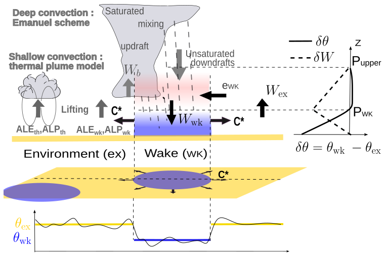
Figure 1Conceptual diagram of the cold pool model and its coupling with convection in LMDZ climate model. (wk) denotes the cold-pool regions, characterized by a lower temperature (θwk), while (ex) represents the environment of cold pools, with a higher temperature (θex). Wwk and Wex denote the vertical velocities in (wk) and (ex), respectively. δθ and δw represent the differences in potential temperature and vertical velocity between regions (wk) and (ex). pwk represents the pressure corresponding to the height of the top of cold pool, defined as the altitude where θwk becomes equal to θex (δθ=0). pupper represents the level at which all cold-pool model variables vanish. C* represents the spreading speed of cold pool. Wb corresponds to the vertical velocity at cloud base. ewk represents the entrainment above pwk. Finally, ALE and ALP represent, respectively, the lifting energies and powers provided by thermals (ALEth, ALPth) and cold pools (ALEwk, ALPwk).
The top height of the cold pool is defined as the altitude hwk (and associated pressure pwk) where the temperature difference between (wk) and (ex) becomes zero. Below this level cold pools are cooler than their exterior. The boundary between the cold pool and the environment is considered to be infinitely thin, and at each point on this boundary, the cold pool spreads at a rate C. C is considered to be a random variable whose mean C* will give the rate at which the cold pool spreads. In the GL10 model, C* scales with the square root of the potential energy available in the cold pools, i.e the energy associated with their collapse, WAPE (Wake Available Potential Energy), given by:
So that:
where ρ is the air density; θv is the virtual potential temperature.
Coefficient k in Eq. (4) should take a value between 0 and 1. Based on 3D CRM (Cloud Resolving Models) simulations, Lafore (2000) estimated this coefficient to 0.33 in the case of a linear structure such as squall line. This is the value retained in LMDZ6A.
When cold pools appear in a grid cell were they were not present before, their fractional cover σwk=πr2Dwk (where r is the cold pool radius) is set arbitrarily to 2 %, corresponding to an initial radius of about 2.5 km over ocean and 30 km over land with the values chosen for the wake number density in LMDZ6A. The cold pool radius then grows with rate so that the time evolution of the fractional area reads:
This surface fraction increases over time. It is limited to 40 % of the domain. When this threshold is reached the growth of the cold pools is stopped and the radius remains constant.
It is assumed that below the top of cold pool (pwk), the vertical velocity profile associated with cold pools results solely from the spreading at the surface, without lateral entrainment (ewk=0) or detrainment (dwk=0) between the cold pool and its environment. Above this level, the subsidence induces a lateral convergence of air feeding the cold pool which can be reinforced by additional re-evaporation of rainfall below stratiform clouds. The shape of the vertical profile of the vertical p-velocity difference δω (where ω is the vertical p-velocity in Pa s−1, while we will note w the vertical velocity in m s−1) between the cold pool region and its environment is imposed as a piecewise linear function of pressure: δω increases linearly from zero at the surface up to a maximum value at pwk and then decreases linearly between pwk and a minimum pressure pupper corresponding to the upper bound of the cold pool model. The vertical subsidence which thus increases downward between pupper and pwk is fed by lateral entrainment ewk without detrainment so that . This lateral entrainment accounts for the horizontal component of the meso-scale circulation known to entrain dry and warm (in terms of potential temperature) air from low- or mid- tropospheric air into the cold pool (see Fig. 1), in turn reducing the WAPE.
At pupper, the top of the cold pool model, δX cancels for all cold pool variables X. In GL10 model and in LMDZ6A, pupper was set to 600 hPa and there was also a nonzero velocity difference (δωcv) at pupper, accounting for the difference of the convective mass fluxes between (wk) and (ex). In the version used here, δωcv=0 above this level as we realized that the GL10 version was introducing a double counting of the vertical mass flux of unsaturated downdraft at pupper. This modification has however little effect on the parameterization results since the mass flux associated with downdrafts at pupper is small (result not shown).
As already said, it is the cooling associated with the re-evaporation of rain in unsaturated downdrafts that is the primary driver of cold pool development. This process is reflected in the model by assigning the heating term computed by the convective scheme to the interior of cold pools, while acts on their environment. Consistent with this splitting, we assume that the saturated part of the convective scheme sees the profiles outside the cold pools, and the unsaturated downdrafts their interior. We further assume that thermal plumes are only active in the fraction of the horizontal surface located outside the cold pools. Thus the mass flux transport scheme is applied to any variable outside the cold pool , and finally and . The thermal plume model therefore induces a differential tendency that is opposite of the average tendency restricted to the environment. Ultimately, the contrast in convective tendencies (shallow and deep) between the cold pools and their environment reads:
It is the terms and that drive the time evolution of δθ and δqv given by:
This time evolution also includes a differential heating and moistening induced by the cold pools themselves of the air inside and outside the cold pools, under the effect of lateral air entrainment from the environment above pwk, subsidence inside the cold pools, and compensating ascent in the environment:
The terms in Eq. (7) partially compensate for the fact that the contrasts δ are not transported by the dynamics until now. We therefore take into account, in the parameterizations, the vertical part of large-scale advection to partially compensate for this deficiency.
Finally, the last term, present only in the θ part of Eq. (7), corresponds to the reduction in temperature contrasts by gravity waves with a coefficient specified as the ratio of an efficiency Kgw to a characteristic time
estimated as the time required for a wave with speed Nz (where N is the Brunt-Väisälä frequency and z is altitude) to travel a distance equal to the geometric mean of the cold pool size and the interval between cold pools.
Finally, the circulation induced in the cold pool parameterizations by the differential heating by convection (and cold pools themselves) contributes as well to the physics tendencies for temperature and humidity. The source terms only contain the vertical convergence of the Reynolds flux associated with mass flux transport (downward in the cold pool and upward in its environment) that reads for any conserved variable ϕ so that:
Finally, the cold pool model includes:
-
three prognostic variables, derived directly from the model equations: the profiles of δθ and δqv and σwk.
-
three diagnostic variables, evaluated from the profile of δθ: pwk, C* and WAPE
-
three main free parameters: the coefficient k, the density Dwk and Kgw.
2.4 Triggering and closure of the deep convection scheme
Triggering and closure formulations in LMDZ have been described in Rio et al. (2013). Deep convection is triggered when the Available Lifting Energy (ALE) at cloud base exceeds the convective inhibition (CIN) threshold. This lifting energy is provided either by the thermal plume model (ALEth) or by the cold pool parameterization (ALEwk):
The intensity of the convection depends on the mass flux (Mb) at the cloud base. The closure consists in expressing Mb as a function of an available lifting power ALP, provided by the thermal plume (ALPth) and cold pools (ALPwk) parameterizations:
where
is the vertical velocity at the level of free convection (LFC), ΔP=500 hPa and wbsrf and wbmax are model free parameters.
Concerning the boundary layer, the available lifting energy is taken as the maximum kinetic energy in the thermal plume below cloud base
A notable improvement was introduced by Rochetin et al. (2014), with the implementation of a statistical representation of the size distribution of cloudy thermal bases. In the new statistical triggering, deep convection is activated if both ALE and at least one cumulus cloud within a grid cell exceeds a given size, specified by Strig (adjustable parameter). The available lifting power scales with .
To calculate ALEwk, the model assumes that the maximum speed (Cmax) on the cold pool contour will trigger convection. This is assumed to be proportional to the square root of WAPE, with a higher coefficient of proportionality than the one used for C* leading to the following relationship:
where .
The Available Lifting Energy associated with cold pools is thus expressed by the following relationship:
Combining Eqs. (16) and (15), one obtains:
with , meaning that, in the cold pool model, the Available Lifting Energy associated with cold pools is equal to the collapse energy.
Each cold pool provides a power associated with its horizontal spreading. This power is calculated as the product of the kinetic energy supplied by the pool and the mass flux, evaluated over the entire contour of the cold pool (Lg=2πr), over the full height of the cold pool hwk, and using the spreading velocity C*. The power (ALPwk,i) of an individual cool pool i is therefore:
To obtain the average power (ALPwk) over all cold pools in the domain, this individual power is multiplied by the cold pool number density Dwk:
Since σwk = Dwkπr2, the lifting power ALPwk reads:
where ϵ=0.25 is the lifting efficiency. This value means that 25 % of the power associated with cold pool spreading is available for deep convection. This rather arbitrary choice is tested hereafter.
2.5 Large Eddy Simulations
Atmospheric Large Eddy Simulations (LES) are performed with non hydrostatic models, with a grid resolution fine enough to resolve the main structures (large eddies) that dominate the turbulent or convective transport. They provide an explicit and detailed representation of turbulent and convective motions within the boundary layer and of the associated clouds (see e. g. Brown et al., 2002; Siebesma et al., 2003, among many others). LES were used as well for assessing parameterizations of deep convection, including cold pools that are represented explicitly in such simulations (see e. g. Suselj et al., 2019). Note however that these simulations can become more dependent on the model parameterizations used when microphysics start to play a predominant role. One of the major strengths of LES lies in its ability to provide three-dimensional information not available from observations, making them an indispensable complement to the latter for understanding processes. In addition, LES can be used to validate the internal variables of parameterizations, enabling their physical realism to be assessed.
In the present study, we use the outputs of LES for two test cases, one over ocean and the other one over land. The test case over ocean was run with two different models, SAM and Meso-NH, with the exactly same setup in order to assess the uncertainty in LES, as it is known that RCE experiments are particularly sensitive to the microphysics scheme (Wing et al., 2018).
The LES over ocean were carried out in Radiative-Convective Equilibrium (RCE) mode (see e. g. Daleu et al., 2015). In the RCE simulations used here, radiative computation is replaced by a constant cooling of −1.5 K per day, while the surface temperature is imposed at 300 K. Two LES of this RCE case are used here, one performed with the SAM model (Khairoutdinov and Randall, 2003) and the other one with Meso-NH (Lac et al., 2018). Both simulations cover an horizontal domain of 200 km × 200 km with resolution of 250 m. The lateral boundary conditions are cyclic for both models. The SAM RCE simulation ran for 44 d, a quasi steady-state regime being reached after about 40 d. SAM output are available every 3 h. The Meso-NH model was first run for 40 d at CRM (2.5 km) resolution and then restarted from the equilibrium reached at 250 m resolution for 10 d. Meso-NH outputs are available every 24 h.
The LES over land is issued from AMMA (African Monsoon Multidisciplinary Analysis) field campaign experiment (Redelsperger et al., 2006). This case is derived from observations made on 10 July 2006 during which a relatively small, short-lived convective system formed over Niamey (Lothon et al., 2011). This system, with a lifetime of around 6 h, was observed by various instruments (radar and atmospheric soundings), supplemented by satellite data. This case study represents a typical example of deep convection in the Sahel region (Couvreux et al., 2012). An LES of this continental case was carried out with the Meso-NH model over a 200 km × 200 km domain, with a horizontal resolution of 200 m. Lateral boundary conditions are cyclic and surface fluxes are imposed. Outputs are generated at a frequency of 30 min.
One advantage of RCE for parameterization development is that it targets a steady state regime. By contrasts, the AMMA case corresponds to a diurnal cycle of deep convection over land, for which the time matters, and for which errors in the phasing of the triggering of deep convection can alter comparisons.
3.1 Distinguishing the cold pools from their environment
In order to use LES for the assessment of the cold pool parameterization, the first challenge is to separate cold pools from their environment. Indeed, there is no a priori established framework for objectively identifying cold pools in observations and numerical models (Rochetin et al., 2021), and choices may depend in part on the physical picture one has of cold pools, and also, for the purpose at hand, on the picture underlying the parameterization. The first method for identifying cold pools proposed by Young et al. (1995) was based on surface precipitation rates. In more recent studies, such as those by Provod et al. (2016); Zuidema et al. (2017); Vogel et al. (2021); Rochetin et al. (2021); Touzé-Peiffer et al. (2022), the detection of cold pools is closer to a density current oriented detection, in which variations in temperature, pressure and wind are taken into account.
In the present study, the aim is not to isolate individual “cold pools objects”, but only to know whether a grid cell of the LES is inside or outside cold pools. Also the boundary conditions are idealized targeting the statistical homogeneity assumption that is at the basis of the Reynolds decomposition between dynamical core and physics parameterizations. In this idealized case with uniform surface temperature, cold pools can be identified using a threshold on the anomaly (after removing the domain average) of temperature at 10 m above surface, T10 m, i.e. at the first model mid layer.
Figures 2 and 3 show a horizontal moving average with a box of 3.25 km × 3.25 km of the divergence of the wind at 10 m above surface, V10 m. From these maps, the centers and gust fronts of cold pools can be easily identified, corresponding respectively to the maximum and minimum of divergence values. Maxima of divergence of surface wind indicate the center of cold pools where cold air masses collapse. Precipitation is generally co-located with these divergence maxima (not shown). The fairly strong wind convergence observed around cold pools centers corresponds to the strong lift of air masses created upstream of the gust front at the cold pool's periphery.
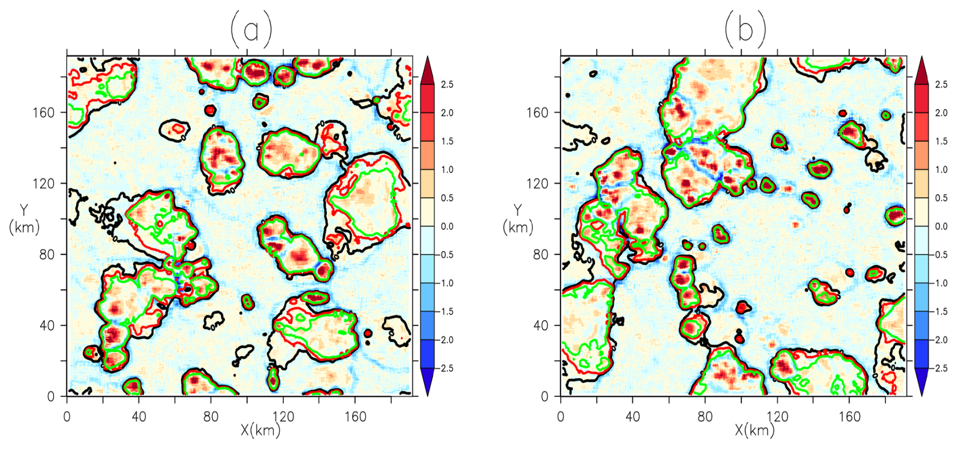
Figure 2Moving average (with a box of 3.25 km × 3.25 km) of the divergence of wind at 10 m (in unit 10−3 s−1 or 1 m s−1 km−1). Panels (a) and (b) correspond to two different states of the LES SAM carried out on the oceanic RCE case. Contours of temperature anomalies at 10 m at −0.4 K (green), −0.2 K (red) and 0 K (black) are superimposed on the smoothed divergence field.
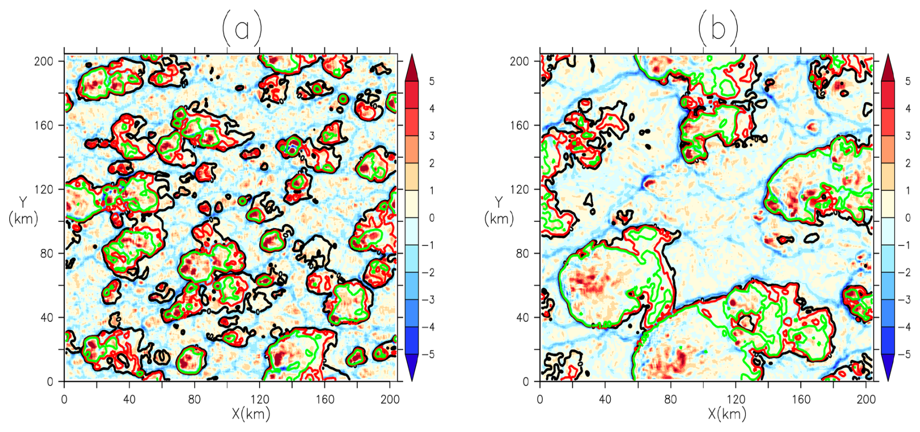
Figure 3Same as Fig. 2 for two successive instants, 5:30 PM (a) and 7:30 PM (b), of the LES Meso-NH carried out on the AMMA case. The contours superimposed corresponds to T10 m anomalies of −1 K (green), −0.5 K (red) and 0 K (black).
Both the two LES of the RCE case and the LES of the AMMA case show cold pools clusters forming a common gust front. This can be explained by the fact that, during propagation, cold pools can merge to create a single, larger cold pool. We can also observe that wind convergence (and thus associated updrafts) is more intense where cold pools meet. This is in line with some studies that indicate that convection initiation on gust fronts is more efficient when two or more cold pools collide (Meyer and Haerter, 2020; Torri and Kuang, 2019; Haerter and Schlemmer, 2018; Feng et al., 2015).
We superimpose on this map the T10 m anomaly contours with different values to determine an optimal threshold for this anomaly. In the RCE case, the T10 m anomaly at 0 K sometimes includes regions without cold pools centers, where divergence of surface wind is low (Fig. 2a and b) while anomaly contours at −0.2 and −0.4 K surround the centers of cold pools quite well. In the AMMA case, figure 3a clearly shows that the 0 K threshold is too high to identify cold pools. Fig. 3b, on the other hand, shows that the −1 K threshold follows gust fronts of cold pools better than the −0.5 K threshold. On the basis of these analyses, we retain the T10 m anomaly thresholds at −0.2 and −1 K to identify cold pools in the RCE and AMMA cases respectively.
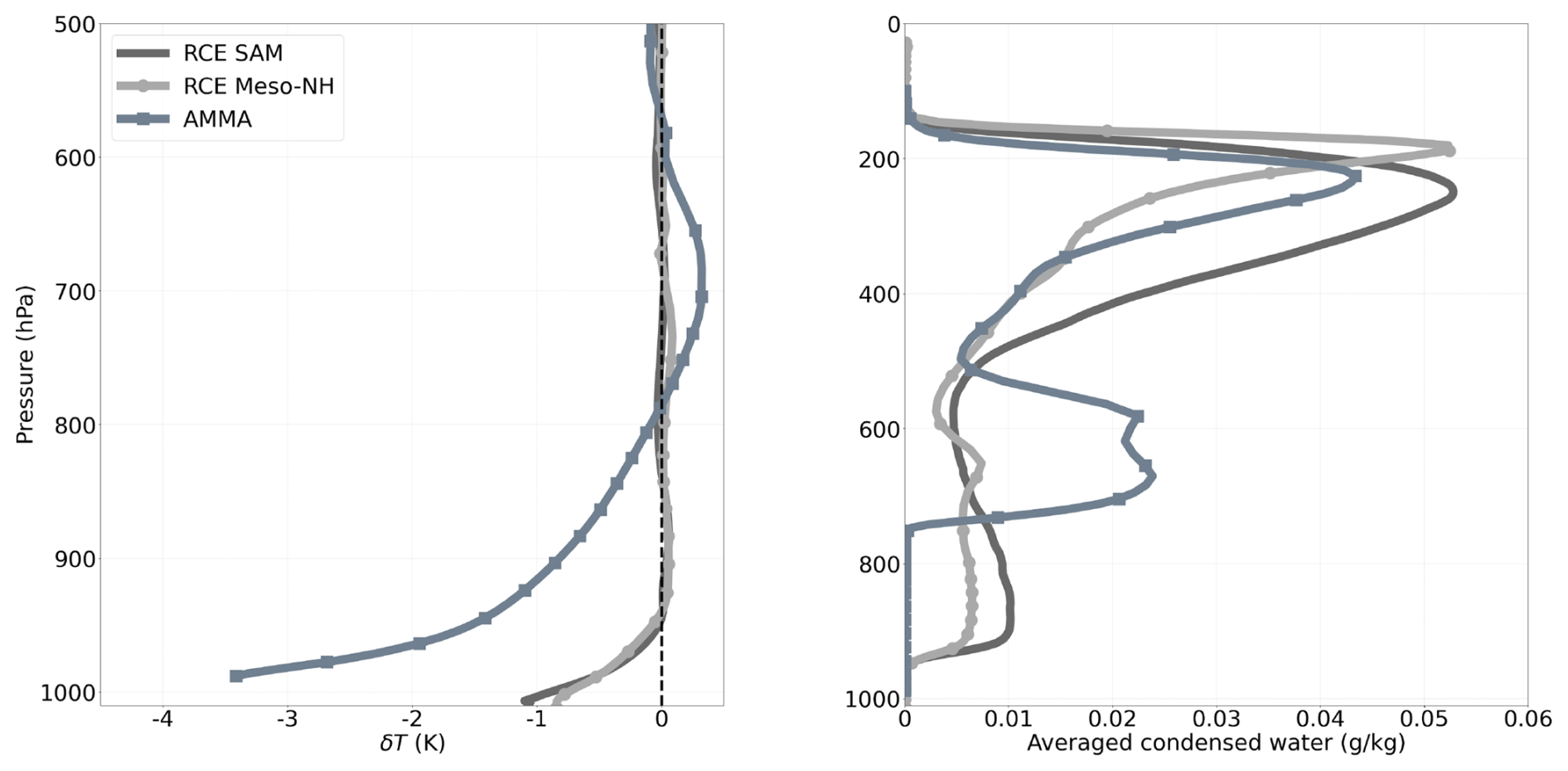
Figure 4Vertical profiles of the cold pool temperature anomaly (left, difference between the inside and the outside of cold pools) and of the averaged condensed water (right, g kg−1).
3.2 Computing the WAPE from the cold pool anomalies
Once the threshold value is fixed for the T10 m anomaly, we separate the full 3-dimensional LES domain between cold pool region (wk) and the rest of the domain (ex) form which we can compute the horizontal averages on each subdomain, Xwk inside cold pools and Xex outside, and then the cold pool anomaly . This sampling allows to compute the vertical profiles of cold pools anomaly for temperature (δT), humidity (δqv) and vertical velocity (δw). Examples of temperature anomalies are shown in Fig. 4.
Note that we apply the same surface mask to the entire column to determine the vertical profiles. This simple vision of vertical cylinders is adopted to match the view underlying the parameterization but may be put into question in the presence of strongly tilted convection.
One can then compute the collapse energy (WAPE) of cold pools in the LES by integrating from the surface up to pwk, the virtual temperature anomaly, δθv (Eq. 3). As suggested by Grandpeix et al. (2010), we take for pwk the pressure where the δT profile cancels out. This altitude is around 950 hPa (approximately 600 m) in the oceanic RCE case and around 800 hPa (approximately 2 km) in the AMMA case (Fig. 4).
3.3 Computing C* from the mean wind divergence inside cold pools
It is assumed in the parameterization that cold pools are identical disks of radius r. This assumption makes it easy to determine C* by the divergence theorem:
After applying Eq. (21), we obtain the following relation
where Swk is the area of cold pools.
Since Lg=2πr, σwk=Dwkπr2 and Swk=πr2, C* can read as a function of the mean divergence of wind at 10 m, the surface fraction (σwk) and the density (Dwk) of cold pools by the relation:
The choice to calculate C* here from σwk rather than from the radius r is explained by the fact that it is easier to estimate σwk in the LES, since we did not use automatic cold-pool detection tools that would allow the radius of cold pools to be determined directly.
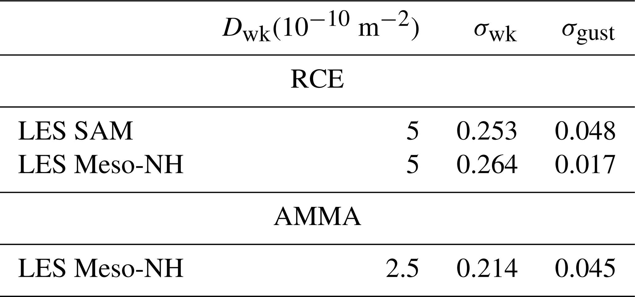
To apply this calculation of C* in the LES, we take the horizontal average of the surface wind divergence inside cold pools. The surface fraction (σwk) of cold pools calculated in the LES is 0.214 (Average over the available time steps between 5:00 PM and 10:00 PM) for the AMMA case and 0.253 (Average over the 24 time steps with the SAM model) for the RCE case. To determine Dwk, we manually counted the centers of cold pools visible on the surface wind divergence maps (Figs. 2 and 3), as we did not use automated detection methods in this study that could generate their number automatically. We find a density, Dwk, of about 5 cold pools per 100 km × 100 km in the RCE case, and about 2.5 cold pools over the same domain in the AMMA case.
3.4 Computing ALP and ALE form gust front vertical velocities
Finally we derive a direct estimation of the Available Lifting Energy (ALEwk) and Power (ALPwk) in the LES from a sampling of the vertical wind at cloud base.
To do this, we first determine an average cloud-base height at which we extract vertical velocities wb(x,y). This height corresponds to the altitude at which the average profile of condensed water reaches its first non-zero value. It is estimated at around 950 hPa on the two LES of the RCE case and at around 750 hPa for the LES of the AMMA case (cf. Fig. 4).
We then separate the updrafts on gust fronts from those associated with thermal plumes. Since the updrafts on gust fronts are both stronger and more coherent horizontally than those associated with thermal plumes, we define a gust front mask based on a threshold applied to an horizontally moving average of the vertical velocity at cloud based wb, denoted as . Because the gust fronts are stronger in the AMMA case than in the RCE case, different choices were made for the size of the horizontal box of the moving average (1.25 km × 1.25 km for the RCE case and 2 km × 2 km for AMMA) and for the value of the vertical velocity threshold (0.6 m s−1 for the RCE case and 2 m s−1 for the AMMA case). Those values were retained after several tests so as to separate as effectively as possible the gust front form other ascents.
Figures 5 and 6 overlays the updrafts within (red) and outside (green) gust fronts on maps of T10 m anomaly (smoothed by applying a moving average with a box of 2.5 km × 2.5 km), for the RCE and AMMA cases respectively. The contours of the T10 m anomalies used to identify cold pools (−0.2 K for RCE and −1 K for AMMA) are displayed as well. Visually, the gust fronts computed with thresholds of 0.6 m s−1 (RCE) and 2 m s−1 (AMMA) align well with the contours of cold pools identified using these T10 m anomaly thresholds. It also appears that most thermals are located in the environment of cold pools for both the RCE and AMMA cases. This retrospectively validates a choice made in LMDZ6A, where the effect of thermals was only computed outside cold pools.
Both ALEwk and ALPwk are computed from wb restricted to the gust front mask, noted wb,gust.
ALEwk is estimated as the kinetic energy associated with the maximum value of :
Table 1Cold pools number density (Dwk), surface fraction of cold pools (σwk), and surface fraction of gust fronts (σgust) estimated from the LES for the RCE and AMMA cases. For the RCE case, the values represent an average over the 24 available time steps from the SAM LES and the 10 available time steps from the Meso-NH LES. For the AMMA case, the values are an average of the time steps obtained between 5:00 PM and 10:00 PM.
ALPwk represents the average updrafts power provided by all cold pools in the domain. It is calculated as the horizontal average of the cube of wb,gust times the surface fraction (σgust) covered by gust fronts:
The gust front mask is used to calculate σgust, which is 0.048 (LES SAM) for the RCE case and 0.045 for the AMMA case, for the times shown in Figs. 5 and 6. Characteristics of the cold pools estimated from the sampling are gathered on Table 1.
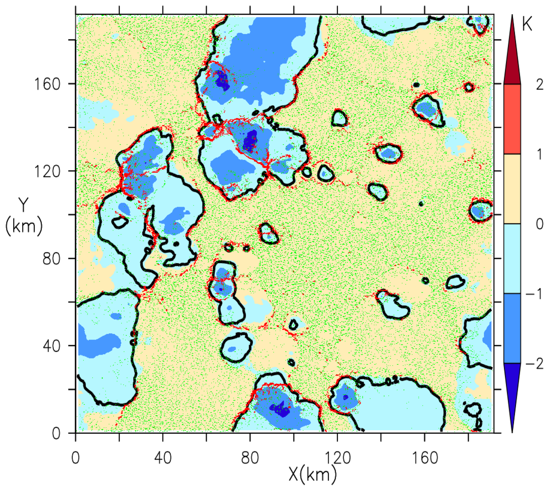
Figure 5Map of T10 m anomaly (color shadings), smoothed (moving average with a horizontal box of 2.5 km × 2.5 km), at an instant of the LES SAM of the RCE case. The black contour is the −0.2 K anomaly used to separate the inside from the environment of cold pools. The green and red dots show grid cells with vertical velocity at cloud base wb larger than 0.8 m s−1, inside (red) and outside (green) the gust front mask (see main text for the definition of the gust front mask).
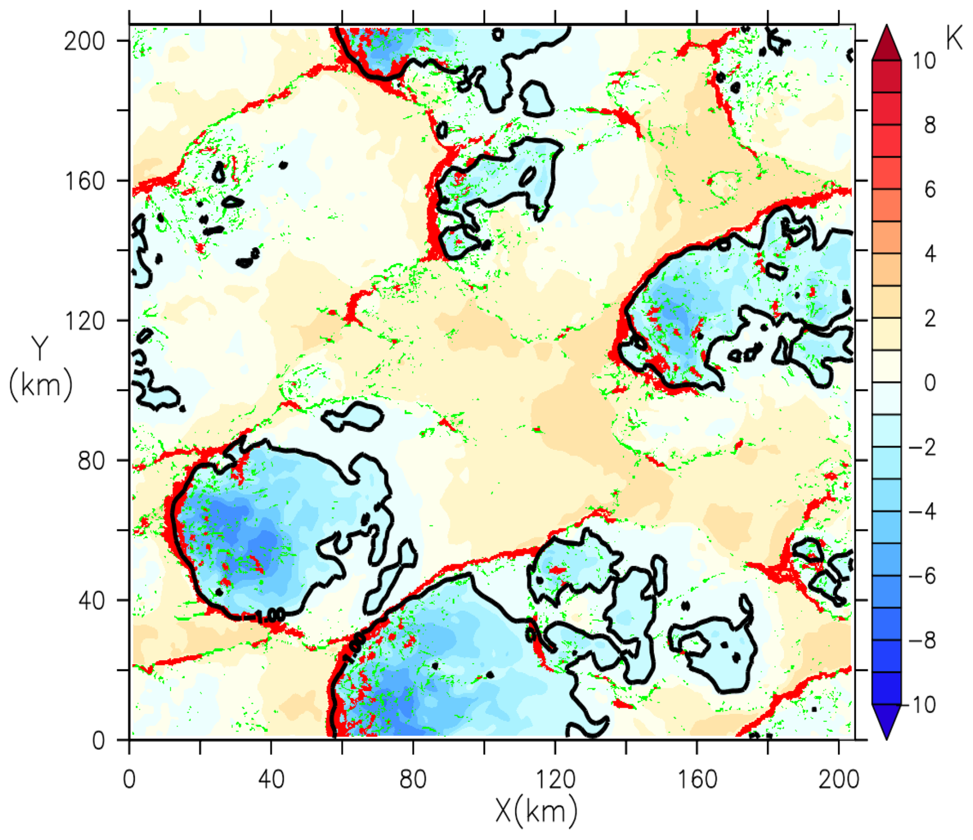
Figure 6Map of T10 m anomaly (color shadings), smoothed (moving average with a horizontal box of 2.5 km × 2.5 km), at 7:30 PM for the LES of the AMMA case. The black contour is the −1 K anomaly used to separate the inside from the environment of cold pools. The green and red dots show grid cells with vertical velocity at cloud base wb larger than 2 m s−1, inside (red) and outside (green) the gust front mask (see main text for the definition of the gust front mask).
3.5 Validation of phenomenological laws
Physical parameterizations are defined by sets of mathematical equations designed to represent subgrid processes within a column of the model. The formulation of these equations is based both on a phenomenological understanding of the processes involved and on fundamental principles of physics. These parameterizations can be evaluated as a whole or in parts, by isolating certain equations or relationships between internal variables, or between internal variables and GCM state variables. LES offers the possibility of performing a priori validation and adjustment of these laws.
In the cold pool model, variables ALEwk, ALPwk and C* are determined from the collapse energy, WAPE (see Eqs. 4, 17 and 20). We compare in Table 2 the values obtained using the parameterization formulations (parameterized value P), based on WAPE deduced from δθv, with those obtained directly from resolved wind in the LES (sampled value S): the vertical speed at cloud base (wb) for ALEwk and ALPwk, and the mean divergence of wind at 10 m in cold pools for C*. These analyses are performed by averaging over the available time steps: 24 time steps for SAM and 7 for Meso-NH in the RCE case, and between 5:00 PM and 10:00 PM for the AMMA case.
The values of ALEwk calculated by both methods are very close to each other. The largest error is an underestimation by about 30 % of the ALEwk computed from WAPE compared to the wb,gust estimate. These results for the three LES confirm the validity of the hypothesis of equality between ALEwk and WAPE assumed in the parameterization.
Table 2Comparison of the variables ALEwk, C*, and ALPwk obtained directly from sampling (S) of the resolved wind in the LES, with those calculated using the formulations of the parameterization (P). The S (bold numbers) values are derived from the vertical velocity at cloud base (wb) for ALEwk and ALPwk, and from the mean divergence of wind at 10 m in cold pools for C*. The P values are calculated from the WAPE deduced from δθv, itself sampled from the same LES. S value of ALEwk are directly compared with WAPE deduced from δθv (Eq. 17). C* and ALPwk of S values are compared with P values of this variables considering the coefficients k=0.33 and k=0.56. The analyses are based on the average of the available time steps: 24 time steps for the LES performed with SAM and 7 with Meso-NH in the oceanic RCE case, and between 5:00 PM and 10:00 PM for the LES of the AMMA case.

Table 2 shows that, C* values computed from the WAPE are systematically lower than those coming from the mean divergence of wind at 10 m in cold pools. This difference could be due to an underestimation of the coefficient k, imposed here at 0.33. With k=0.56, the calculation of C* based on the WAPE becomes comparable to those obtained from the mean divergence of wind at 10 m in cold pools (Table 2). As discussed above, the value of 0.33 was retained following an oral communication by Lafore (2000). But other studies propose different values: Lafore and Moncrieff (1989) estimate k at 0.68 based on CRM simulations of 2D squall grain, Bryan (2005) estimate it at 0.5 from observations of cold pools during the BAMEX experiment in the American Great Plains. Our results are thus compatible with the hypothesis of the model which postulates that the kinetic energy of cold pools results from the transformation of WAPE into kinetic energy with a coefficient k compatible with the published estimates.
Table 2 also shows that, for the three LES cases, the values of ALPwk calculated with C* from WAPE are at least three times lower than those obtained from wb,gust. Two coefficients are involved in the calculation of ALPwk with the parameterization formula: the coefficient k and the lifting efficiency ϵ, imposed respectively to 0.33 and 0.25. Using k=0.56 however in the calculation of C*, and keeping ϵ at is nominal value of 0.25 allows to reconcile the various estimates. This is compatible with the hypothesis of the parameterization according to which 25 % of the horizontal power provided by the cold pools during its propagation would be used to reinforce the intensity of the convection while a large part dissipates.
In this section, we evaluate the cold pool parameterization in the SCM configuration of LMDZ. The comparison is more demanding here, since all parameterizations interact with each other and because the state of the atmosphere at the time of evaluation depends on the interaction of all those parameterizations during the preceding hours (AMMA) or days (RCE). The SCM simulations are performed with exactly the same initial and boundary conditions as the corresponding LES for both cases.
For the RCE case, we represent diagnostics once a quasi-steady state has been reached by averaging results between day 40 and 44.
In the AMMA case, cold pools appear around 5:00 PM in the LES but as early as 1:30 PM in LMDZ CTRL, revealing a model limitation. Adjusting the Strig parameter involved in the triggering criteria could delay this onset, though a more physical approach would be required. For comparison, we focus on the times when cold pools are most developed: 7:30 PM in the LES and 2:30 PM in LMDZ CTRL, where the intermediate analysis of δT shows colder and thus more pronounced pools.
In order to facilitate comparisons between LMDZ and LES, we also impose in the LMDZ simulations the density of cold pools estimated in the LES. We thus set a density of 5 cold pools per 100 km × 100 km for the RCE case and 2.5 cold pools per 100 km × 100 km for the AMMA case. To represent the profiles of δT, δqv and δw in LMDZ CTRL for the RCE case, we perform a time average between the 41st and 43rd day of simulation, in order to compare with the LES at the same times. For the AMMA case, the analysis is performed at 7:30 PM in the LES and at 2:30 PM in LMDZ CTRL, as specified above. The same procedure is applied to compare the WAPE, ALE, and ALP variables between LMDZ CTRL and the LES for both cases.
4.1 Vertical profiles of δT, δqv and δw
The analysis of the δT profiles in the LES confirms that cold pools are colder at the surface with temperatures increasing towards the top for the three LES. The cold pools are about three times deeper in AMMA (Fig. 7a) than for the RCE case (Fig. 7d). In the LES, the cold pool temperatures for the AMMA case (around 4 K) are lower than those of the RCE case (around 1.2 K). This is consistent with observations which indicate much colder pools over land than over the ocean. For the AMMA case in particular, observations reveal a temperature drop of approximately 5 K during the passage of the cold pool (Lothon et al., 2011), a value fairly close to that of the LES. It should be noted however that the AMMA case corresponds to a relatively weak episode of continental convection. The δqv profiles indicate that at the surface, cold pools are wetter than the surrounding air in the RCE case and the AMMA case (Fig. 7b and e). In both cases, the excess of humidity within cold pools decreases with altitude up to the cold pools top. The humidity deficit above this level is due to the lateral entrainment of dry air from the mid troposphere and its subsidence into the cold pools (Fig. 7c and f). For the RCE case, this subsidence vanishes below 800 hPa (Fig. 7c), while for the AMMA case, it vanishes at a higher level, around 600 hPa (Fig. 7f).
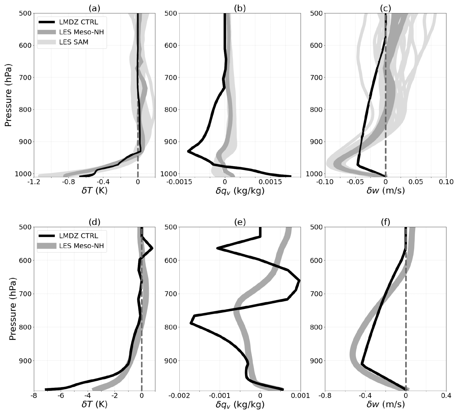
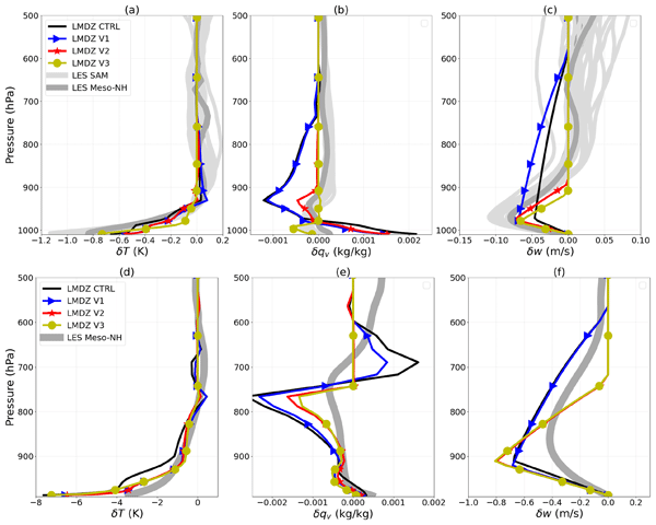
Figure 7Vertical profiles of δT, δqv and δw calculated in the LES and simulated by LMDZ control (LMDZ CTRL). For the RCE case (a, b, c), the profiles are shown for a set of 24 times for the SAM LES (light grey) and 10 for Meso-NH (dark grey). For LMDZ CTRL, results are averaged from day 41 to 43. For the AMMA case (d, e, f), the profiles correspond to the times when cold pools were most developed, i.e., 7:30 PM in LES and 2:30 PM in LMDZ CTRL.
The δT profiles simulated with LMDZ CTRL are qualitatively consistent with LES, with a cold pool top (where δT cancels) at about the right altitude. Cold pools simulated with LMDZ are however warmer than in the LES for the RCE case (Fig. 7a), and colder at the surface than the LES for the AMMA case (Fig. 7d). Consistently with LES, cold pools are also wetter at the surface and drier close to their top top (Fig. 7b and e). However the variations of δqv are much larger in LMDZ than in the corresponding LES. In particular, the cold pools are much too dry at their top in LMDZ. In both cases, cold pools are associated with subsidence. The height at which the subsidence of air masses into cold pools begins, fixed at 600 hPa in LMDZ CTRL, is too high compared to LES for the RCE case (Fig. 7e).
4.2 WAPE, ALE and ALP
Table 3Comparison of the WAPE, ALEwk, C* and ALPwk computed from sampling of the LES and by LMDZ control (LMDZ CTRL) for the RCE case and the AMMA case. For the RCE case, comparisons are made using an average of the days following the achievement of equilibrium (days 41, 42, and 43). For the AMMA case, they are performed at the times when the cold pools are most developed (7:30 PM in the LES and 2:30 PM in LMDZ CTRL).
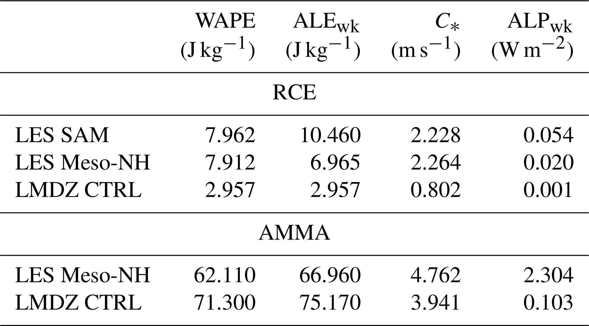
For the RCE case, the WAPE is significantly smaller in LMDZ CTRL than in the LES, with a difference of at least a factor of 2 (Table 3). These low values of WAPE in LMDZ CTRL also translate into low ALEwk values compared to LES (Table 3). On the other hand, for the AMMA case, the WAPE simulated by the model, and consequently ALEwk, are slightly higher than the values derived from the LES (Table 3). The value of C* simulated by LMDZ CTRL is at least three times smaller than that of the LES in the RCE case and slightly lower for the AMMA case (Table 3). ALPwk is at least twenty times weaker in LMDZ CTRL than in the LES for all cases (Table 3).
Various modifications of the cold pool parameterization are explored in the following section to try to correct the defects listed above.
Here, we start by correcting the identified discrepancies between the LES and the model concerning the value of the coefficient k and the pressure height pupper, and by assessing the impact of these changes on the temperature and humidity difference between the cold pools and their environment, before exploring other avenues for improvement.
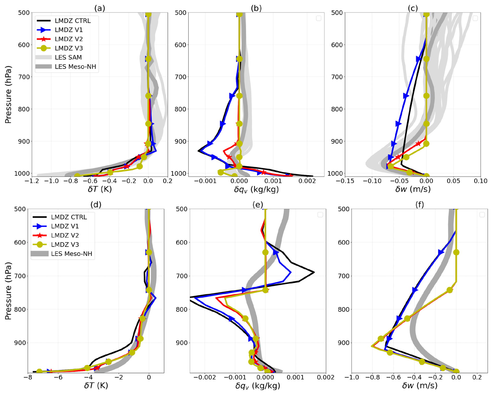
Figure 8Vertical profiles of δT, δqv and δw calculated in the LES and simulated with LMDZ: for a control simulation (CTRL, same curves as Fig. 7), with adjustment of the coefficient k to 0.56 (V1), with the modified computation of pupper (V2) and with the activation of thermals in the entire domain (V3). Both the RCE (a, b, c) and AMMA (d, e, f) cases are shown for the times as in Fig. 9.
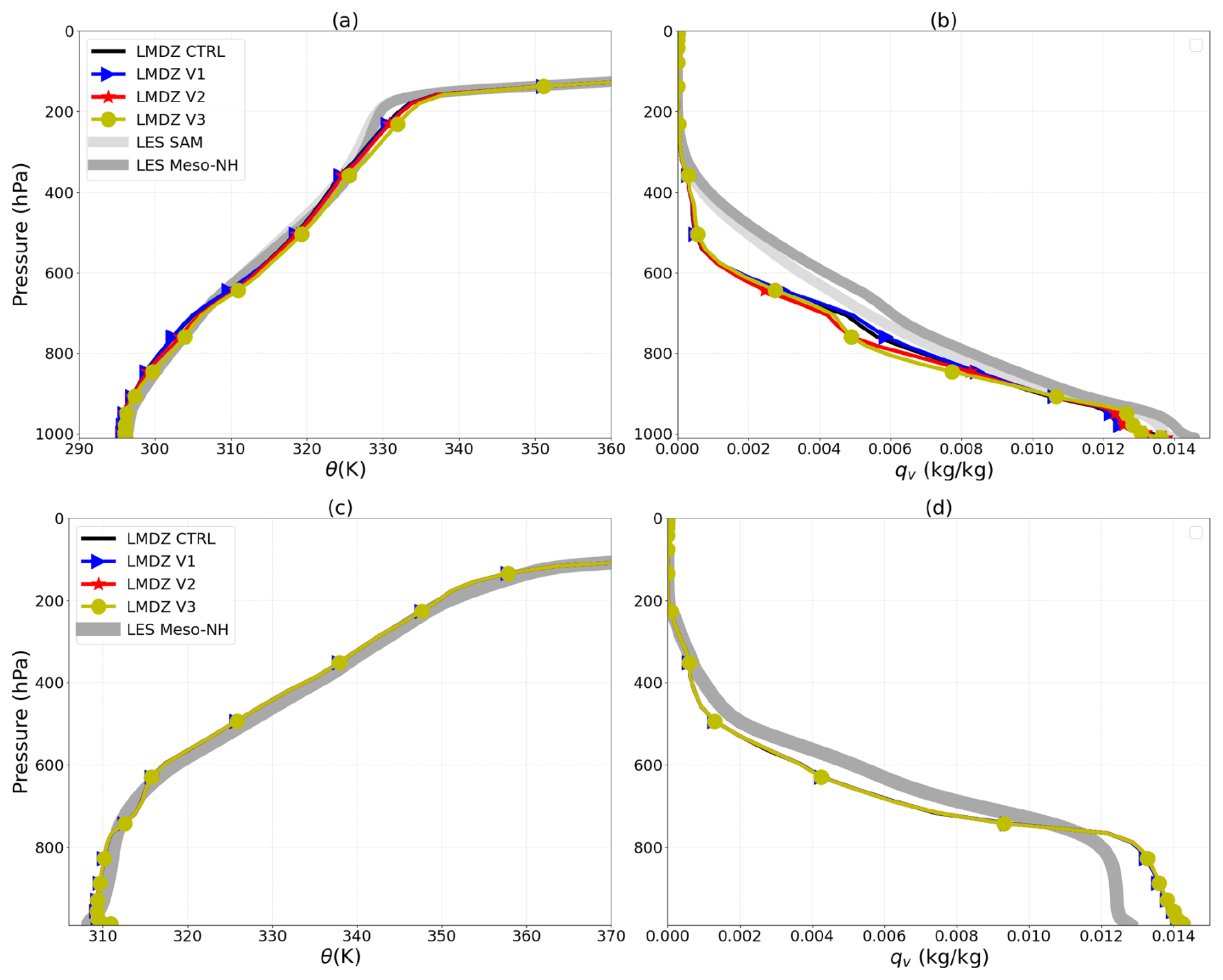
Figure 9Vertical profiles of potential temperature (θ) and specific humidity (qv) calculated in the LES and simulated with LMDZ: for a control simulation (CTRL), with adjustment of the coefficient k to 0.56 (V1), with the modified computation of pupper (V2) and with the activation of thermals in the entire domain (V3). Both the RCE (a, b) and AMMA (c, d) cases are shown for the same times as in Fig. 7.
Table 4Description of simulations performed with LMDZ in the standard configuration and with various modifications.
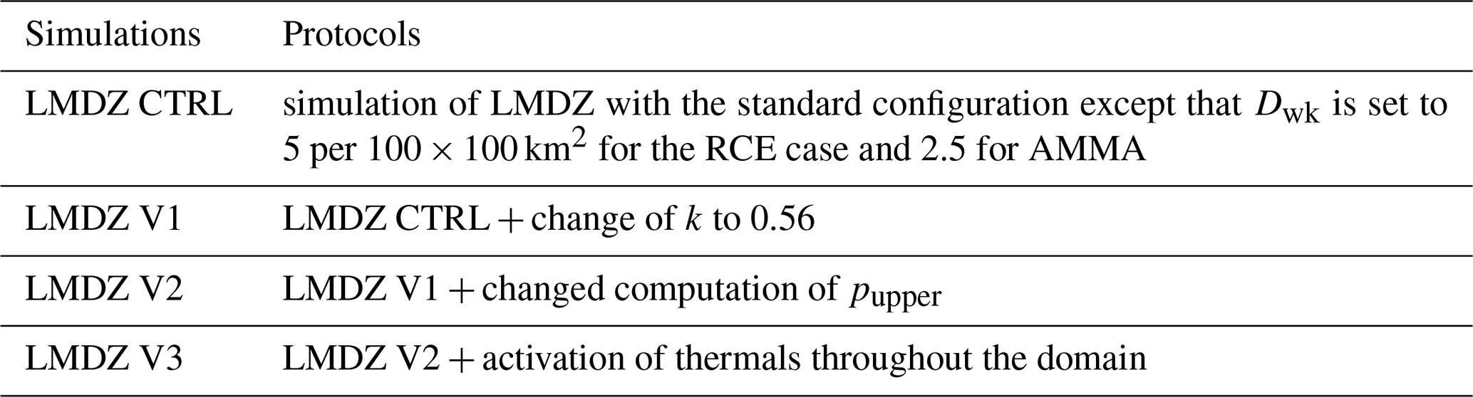
5.1 Coefficient k
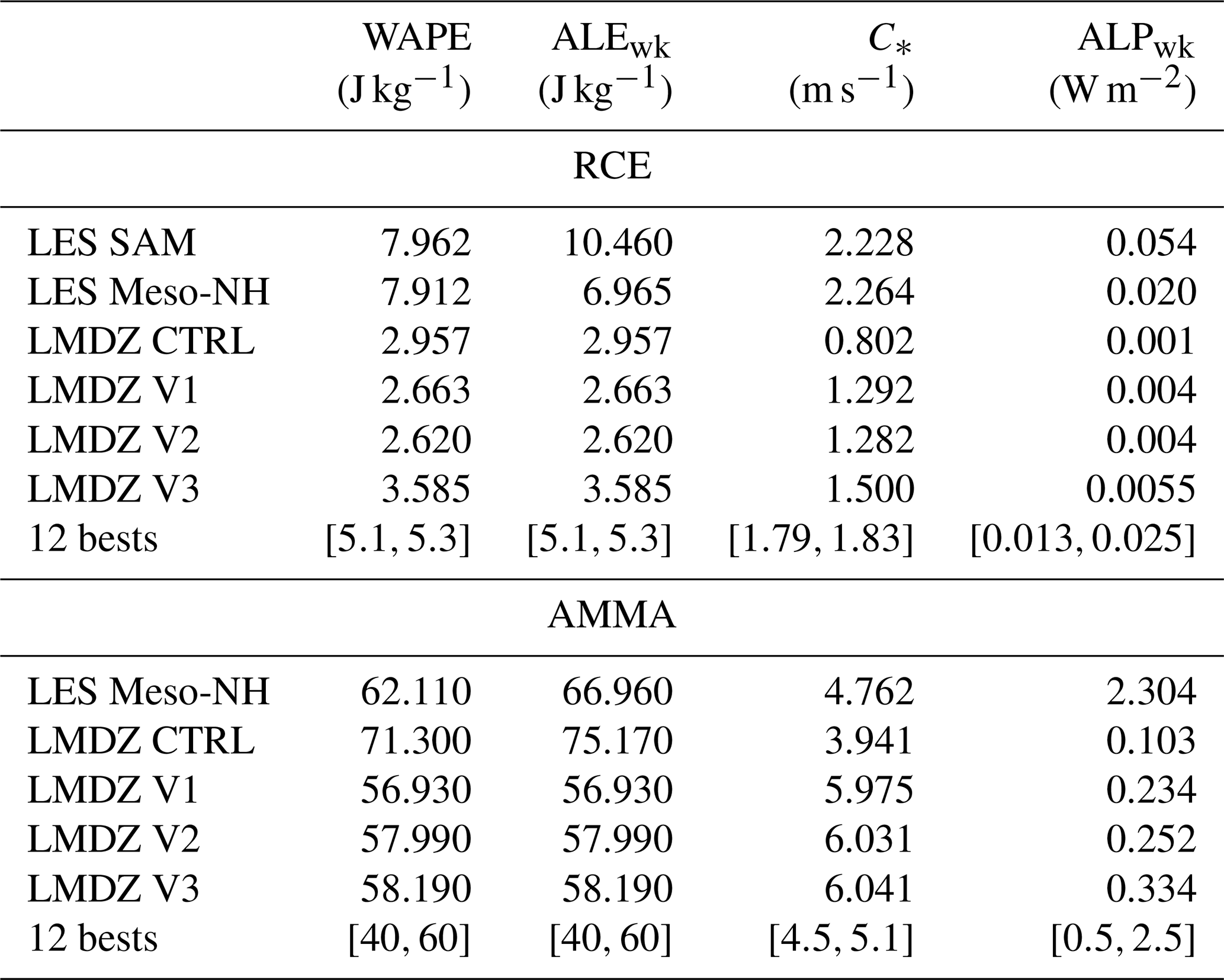
We present here the impact of increasing the coefficient k from 0.33 to 0.56 (LMDZ V1 simulation) on the profiles of δT, δqv, δw as well as on the variables C*, WAPE, ALPwk and ALEwk (see Table 4). In the RCE case, this modification significantly improves the profile of δw below pwk (Fig. 8c). It also allows for a better representation of the δw profiles below pwk in the AMMA case (Fig. 8f). These improvements are directly linked to the increase in C* for both cases (Table 5), since the δw profile below pwk depends on the spreading of cold pools. The increase in C* could be associated with stronger air mass subsidence within the cold pool, which would contribute to a slight drying near the surface in both cases (Fig. 8b and e). For the AMMA case, this drying results in slightly drier cold pools at the surface in LMDZ V1 than in the LES, but they remain overall comparable to the latter. The increase in C* in both the RCE and AMMA cases also leads to a better representation of ALPwk (an increase by at least a factor of 5 for both cases), even though this variable remains underestimated (Table 5). We also note a warming effect from this modification in both the RCE and AMMA cases. The impact on the δT profiles in the AMMA and RCE cases is responsible for the decrease in the values of WAPE and ALEwk for these two cases (Table 5).
Figure 9 shows that the modification introduced in version V1 has a low impact on the θ and qv mean profiles (Fig. 9), the black and blue curves being almost superimposed. Both CTRL and V1 simulations reproduce the θ profiles fairly well. Around 600 hPa, the temperature is too warm in the RCE case. Regarding humidity, a dry bias is present in the boundary layer in the RCE case, as well as between 800 and 400 hPa. For the AMMA case, there is a wet bias in the boundary layer and above 600 hPa, and a dry bias between 700 and 600 hPa. At the altitudes where these dry biases are found, notably between 800 and 400 hPa for the RCE case and between 700 and 600 hPa for the AMMA case, LMDZ produces almost no clouds, likely due to an overly dry atmosphere (not shown).
5.2 Choice of cold pools scheme upper bound, pupper
In the previous sections, we found that the altitude at which the subsidence of dry air above cold pools initiate is located around 800 hPa in the LES for the RCE case and around 600 hPa for the AMMA case, while in LMDZ, pupper is arbitrarily set to 600 hPa in the original version of the parameterization. In version V2, in addition to the change of the value of k from 0.33 to 0.56, we impose where γwk,upper (fixed here to 3) is considered as a new free parameter in the following section.
Note that the numerical scheme used to estimate pwk was also modified compared to GL10 in order to solve instability issues.
The principle of the new scheme is to compute the height at which the vertical integral of δθ, from the surface to that level, reaches a fraction χ of the total integral from the surface to the first positive value of δθ. This fraction is taken slightly below 100 % to avoid fluctuations of pwk from one time step to the other, which happens when δθ is close to zero on a large range of altitudes around pwk as seen in Figs. 7 and 8. The new computation was activated already in CTRL and V1, not affecting the results significantly (figure not shown). The new computation becomes really important when pupper is deduced from pwk rather than being imposed.
Comparisons between LMDZ V2 simulations and LES show a better representation of the δqv profiles at the top of cold pools in both the RCE and AMMA cases (Fig. 8b and 8e). These results show that the dry bias at the top of the cold pool in the original version was due to advection of dry air from too high an altitude. This modification also reduces slightly the humidity of cold pools near surface in the RCE case, although they remain more humid than in the LES. Note finally that this modification has a very limited impact on the δT profiles.
Table 5 shows that the change in pupper weakly affects the variables WAPE, C*, ALEwk and ALPwk for these two cases.
Versions V2 does not modify much the mean vertical profiles except for a drying of the mid-troposphere in the RCE case (Fig. 9b), in a region where the CTRL simulation was already too dry. Although the time evolution of the mean profiles is the first target of physics parameterizations, we think however that the improvement of the internal variables is so strong for this modification that it should be adopted in the future in LMDZ.
5.3 Activation of thermals throughout the domain
As explained above, in the standard LMDZ configuration, thermals only interact with temperature and humidity profiles outside cold pools, inducing a differential heating in moistening (Eq. 6). This choice was originally made to account for the fact that the atmosphere is more stable inside cold pools, and indeed the analysis above shows that the thermal plumes that reach cloud base are essentially located outside cold pools. Version V3 is identical to version V2, except that we consider that thermal plumes are active everywhere in the grid cell. Consistently, the terms and are removed from Eq. (6). For the RCE case, this leads to a decrease in the surface humidity of cold pools, closer to the LES results (Fig. 8b). In the AMMA case, the effect is also present, although less pronounced (Fig. 8e). This result is expected because the vertical transport by thermals systematically dries the surface (Diallo et al., 2017). This confirms the key role of boundary layer convection in regulating surface humidity on both continent (Diallo et al., 2017) and ocean (Hourdin et al., 2020b), via the mixing of moist air with dry air above. One way to improve the representation of humidity anomaly profile without activating the thermal plumes everywhere would be to add a simple parameterization of shallow and cloud-free boundary layer convection (a simplified version of the thermal plume model) within the cold pool region.
In version V3, cold pools are colder than in version V2 in both the RCE and AMMA cases (Fig. 8). In the RCE case, however, cold pools remain less cold than in the LES despite this effect. In the AMMA case, this cooling accentuates the overestimation of the cold anomaly. In both cases, this cooling leads to an increase in the WAPE, C*, ALEwk, and ALPwk variables (Table 5). Version V3 does not introduce any notable changes, compared to V2, in the profiles of θ and qv for the RCE and AMMA cases.
Table 5Comparison of the variables WAPE, ALEwk, C* and ALPwk calculated from the samplings in the LES, with those obtained with LMDZ: in a control simulation (CTRL), with the adjustment of the coefficient k to 0.56 (V1), with the modified computation of pupper (V2), the activation of thermals in the entire domain (V3) and for the 12 best simulations of a tuning experiment, for the RCE and AMMA cases.
5.4 Tuning of free parameters
The tests presented above show possible avenues for improving the cold pool parameterization. However, we see that the modifications do not sufficiently affect the mean profiles to reduce these biases significantly. All tests underestimate (for the RCE case) or overestimate (for the AMMA case) the cold temperature anomaly inside cold pools, as well as WAPE, ALEwk, C*, and ALPwk. We also observe systematic errors in the mean profiles, notably profiles that are much too dry for the RCE case.
In the GCM, these variables are not sensitive only to the parameters or formulation of the cold pool model. They are influenced by all other parameterizations, and in particular by the convection scheme to which the cold pool scheme is strongly coupled. In an attempt to see how modifications to other parameterizations could help reduce these biases, we performed automatic calibration simulations using the htexplo tool.
In practice, we decided to start from a tuning performed for the convective boundary layer by Hourdin et al. (2021), for a configuration with 95 levels rather than 79 and using more recent versions of the codes than those used in the rest of the paper. This version indeed serves as the basis for preparing the future version of the climate model for the Fast-Trac part of the CMIP7 project, whose simulations are scheduled to begin in early 2026. We assume that the boundary layer parameters values have already been chosen to accurately represent the convective boundary layer and associated clouds, cumulus and stratocumulus. Regarding modifications to the cold pool model, those affecting the coefficient k and pupper are taken into account, as in the V2 configuration. Adjustments related to thermals (V3) are not considered here because they raise as many questions as they solve.
The tuning is performed using the htexplo tool as explained in Appendix A. We choose metrics preferentially on the RCE case targeting the WAPE, ALP and the profiles of anomalies and mean variables. Indeed, we wish to avoid being overly dependent on errors in the phasing of the deep convective diurnal cycle. The adjustable parameters selected for the cold pool model are: k, γwk,upper, χ, and ϵ. Parameters involved in the deep convection scheme are also included: the minimum wbsrf and maximum wbmax vertical velocities at the base of the convective column; the fraction of the grid cell area in which precipitating downdrafts occur, σdesc; and the maximum precipitation efficiency in the Emmanuel scheme (EPmax). This efficiency is a maximum efficiency at the top of the convective columns. The difference 1−EPmax controls how much condensed water exits the convective clouds, and thus the moisture source in the upper atmosphere. Details on the metrics and parameter ranges chosen are given in Appendix A.
The result of this tuning is the product of trial and error preliminary tuning experiments regarding the choice of parameters, their bounds, the metrics to adjust, and the associated tolerances. We finally perform 13 waves of tuning with the experimental setup described in Appendix A, and present here the 12 best configurations among all the runs performed during this tuning experiment. The best simulations are selected according to the 13 metrics involved in the tuning procedure (cf. Table A1). For each metric we compute a score where mi is the metrics computed on the simulation, oi the target value (“observation”) and σi a tolerance to error. A combined metric is computed as the maximum of si over the 13 metrics: Si=maxisi. The best simulations are those with the smallest values of Si.
The analysis of the results for the RCE case reveals that the 12 bests configurations better simulate the targeted variables, particularly the mean humidity profile and the amplitude of the potential temperature deviations δθ. These deviations are more negative, consistent with a stronger WAPE and C* coefficient. Furthermore, the δqv profiles at the top of the cold pools, as well as the δw profiles, remain well represented across all 12 simulations.
By applying the parameters from the tuning performed on the RCE case to the AMMA case simulations, a significant reduction in the cold bias at the surface of cold pools is obtained (Fig. 10d), as well as an improvement in the mean humidity profiles across all 12 simulations. Only the best simulation (BEST TUNE) reproduces δqv and δw profiles consistent with the LES, the others tending to generate cold pools that are too dry at their top due to slightly overestimated δw profiles (Fig. 10e and f). The BEST TUNE simulation also provides a better representation of WAPE (Fig. 12a) and ALPwk (Fig. 12b) in the AMMA case, with values very close to those from the LES at the time when cold pools reach their maximum development (Table 5), despite a shift by about 3 h earlier in the afternoon.
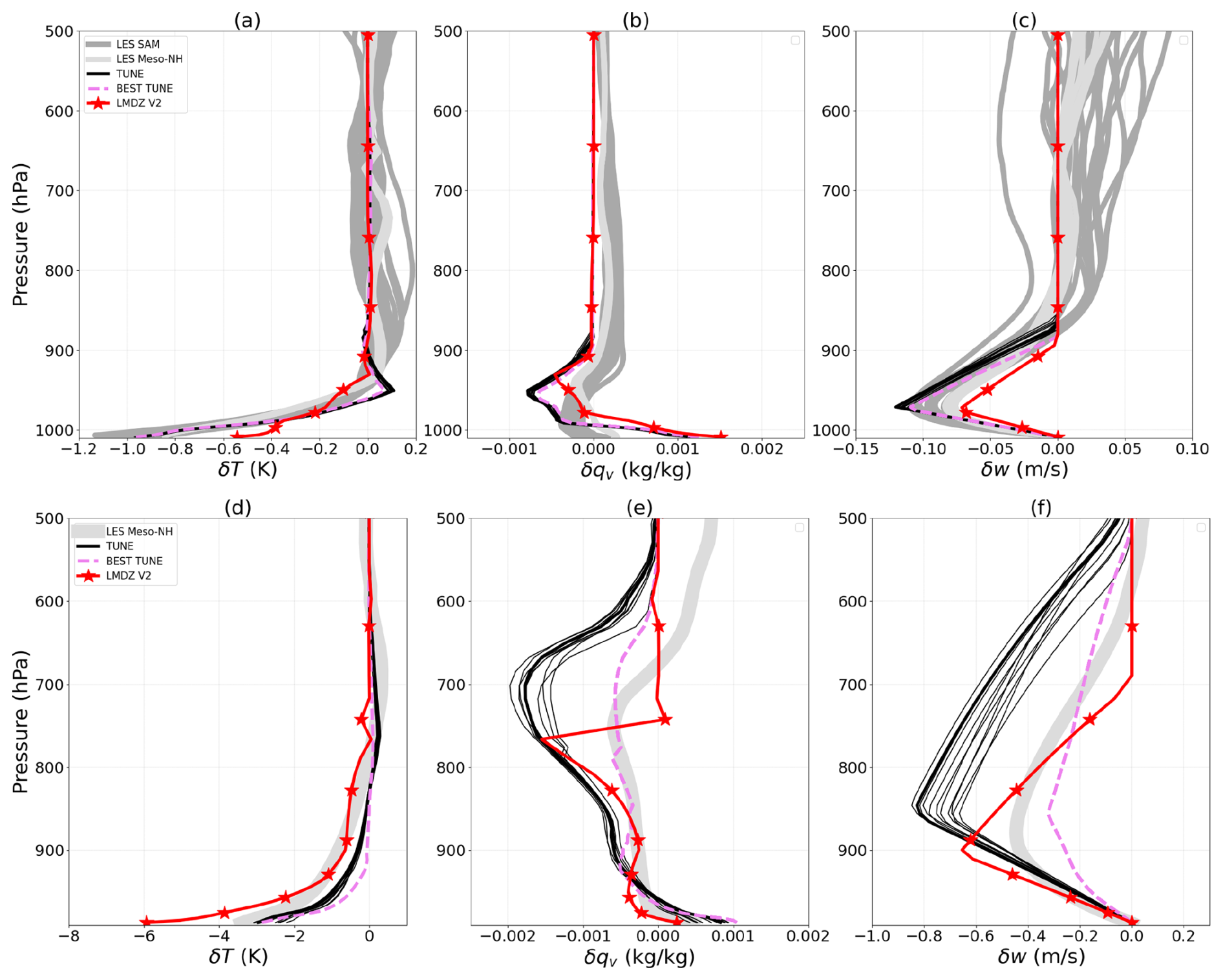
Figure 10Like Fig. 8, but showing for LMDZ, the V2 simulation, the 12 best simulations from the tuning (TUNE, in black) as well as the best one among them (TUNE BEST, in violet dotted).
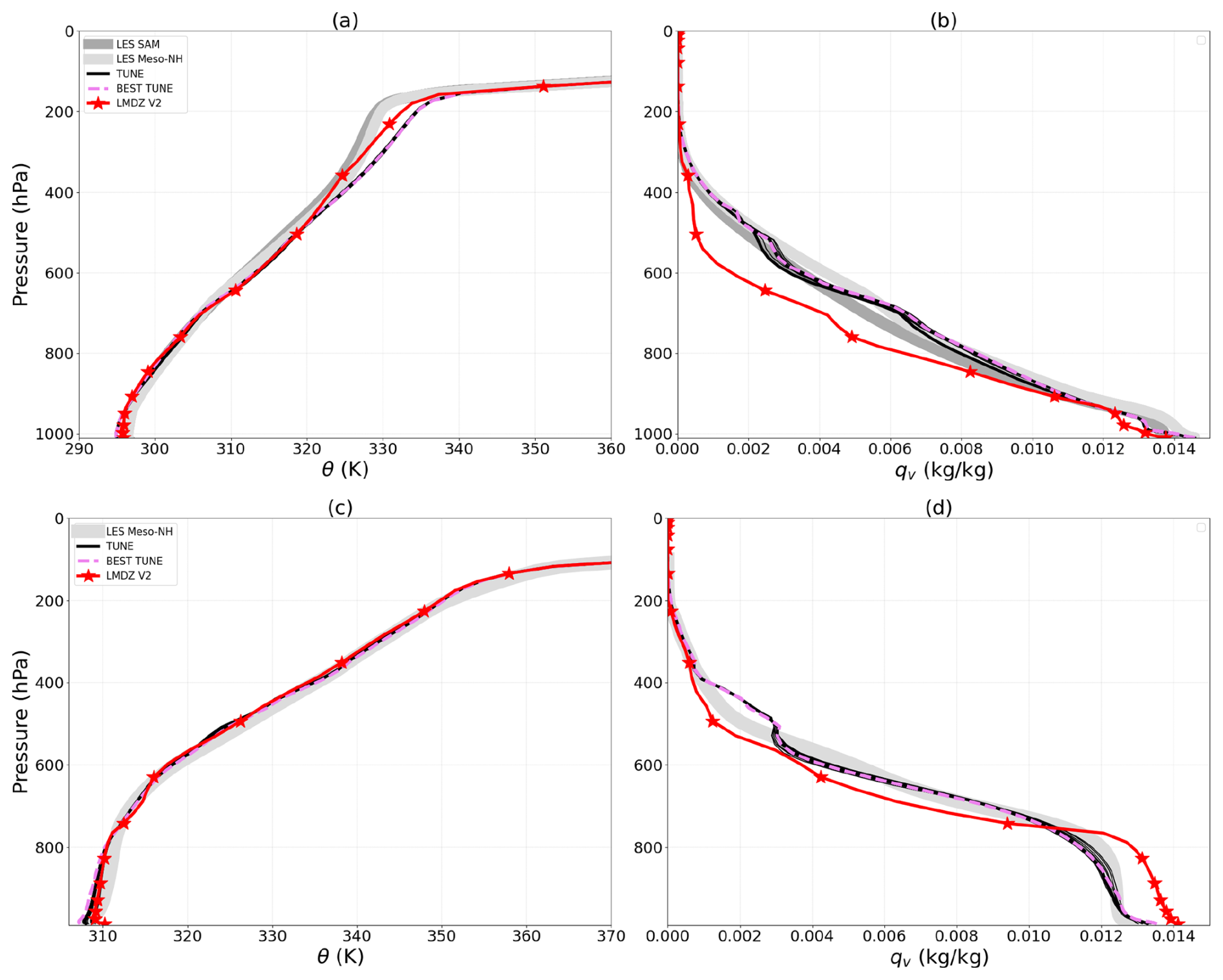
Figure 11Like Fig. 9, but showing for LMDZ, the V2 simulation, the 12 best simulations from the tuning (TUNE, in black) as well as the best one among them (TUNE BEST, in violet dotted).
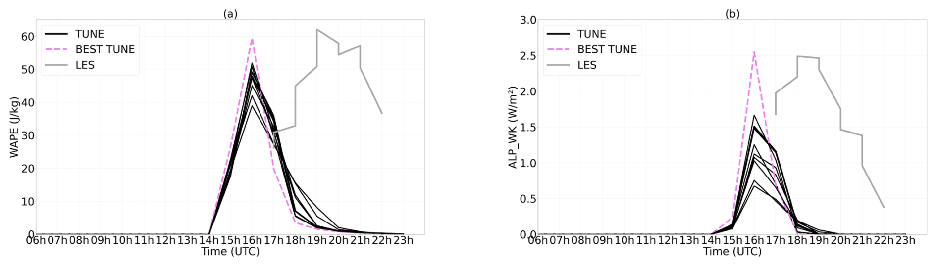
Figure 12Time series of the collapse energy, WAPE (J kg−1, panel a), and the available lifting power,ALPwk (W m−2, panel b), associated with cold pools, shown for the 12 best simulations from the tuning (TUNE, in black), for the best among them (TUNE BEST, in violet dotted) and for the LES (in grey) over times steps between 5:00 PM and 10:00 PM.
It is well known that representing the diurnal cycle of convection remains a major challenge for GCMs. In LMDZ, a significant improvement in the representation of the diurnal cycle of precipitation was achieved thanks to the preconditioning of convection by thermals, as well as the role of cold pools in sustaining convection (Rio et al., 2009). Nevertheless, the delay in the timing of convective initiation remains a limitation. Intermediate tests have shown that tuning the parameter Strig, which defines the threshold cumulus size required to trigger deep convection, can delay convective onset. A work aiming at better representing the transition between shallow and deep convection is currently ongoing in the LMDZ team.
Several lessons can be learned about the range of the free parameters involved in the tuning when considering the best values (last column of Table A2).
First the fraction of the grid cell assigned to unsaturated downdrafts, σdesc with a selected range of [0.042,0.048], is larger than the nominal value of 0.003, which contributes to first order to the increased intensity of cold pools, in particular for the RCE case. Concerning the parameters of the cold pool model itself, first the tuning of k from Eq. (4) confirms the findings of Sect. 3.5, with selected range of [0.56,0.57]. The value of γwk,upper that controls the height of the cold pool model is [3.6,4.1], compatible as well with the previous findings. With a range of [0.26,0.46], the tuning suggest that more than 25 % of the power associated with cold pool spreading is available for deep convection. Note finally that the χ parameter of the new numerical scheme for pwk computation is also strongly constraint by the tuning exercise (to a value of about 0.97). The values of parameters in the control simulation (initial values) and in the BEST TUNE simulation are presented in Table A2.
The htexplo tool retrieves automatically cold pool model parameter values close to those issued from direct analysis of LES. This highlights both the power of using such a tool for model development, avoiding a long phase of trial error in a multi-dimensional space, and the relevance of the model physics. Likewise, the range of values selected for σint leads to cold pool heights of about 600 m in the RCE case and 2 km in the AMMA case, in agreement with the expected orders of magnitude over ocean and over land, respectively.
One goal of the tuning is to intensify cold pools, particularly in the RCE case. The increase of σdesc is primarily responsible for strengthening cold pools in this case, through stronger evaporation.This increases confidence in the validity of the physics implemented in the cold pool model. In the AMMA case, the opposite effect (less colder cold pools) is explained by the rather large increase in C* (from 3 to 5 m s−1), induced by the adjustment of k. This increase in C* accelerates the increase of the cold pools fractional area σwk, reducing the efficiency of evaporative cooling, which can no longer compensate for the dilution due to their rapid evolution. Although this mechanism is also present in the RCE case (with an increase in C* from about 1 to 2 m s−1), it remains much less pronounced there, allowing the evaporation obtained with these σdesc values to effectively strengthen the cold pools.
We also consider that the increase of the difference 1−EPmax and σdesc played an important role in the improvement of the specific humidity profiles for the RCE and AMMA cases, although other parameters may also play a role. The increase of the difference 1−EPmax increases the amount of condensed water released at the top of the convective columns, thereby moistening the upper layers of the atmosphere. The value of EPmax was set to 0.999 in the control configuration. The increase in σdesc may both enhance humidity through enhanced evaporation and dry the boundary layer, for the AMMA case in particular, due to increased entrainment and downward advection of dry air from the free troposphere.
We also briefly examined the behavior of updrafts, given their strong coupling with downdrafts and cold pools. We note a decrease in undiluted adiabatic updrafts (which represent the theoretical capacity of the column to transport air and moisture) and a decrease in saturated updrafts in the tuned simulations (not shown). These effects are more pronounced in the AMMA case. The decrease in undiluted adiabatic updrafts would be linked to the drying of the boundary layer, itself associated with the increase in σdesc, as explained previously. This reduction in undiluted updrafts would also contribute to the decrease in saturated updrafts by limiting the moisture supply to the mixing with environmental air.
This study presents an evaluation of the LMDZ cold pool model based on Large Eddy Simulations (LES). We evaluate both the fundamental assumptions of the model, the properties of the cold pools it simulates, as well as its coupling with deep convection, using LES of two test cases: the RCE case offers a controlled and quasi-stationary framework for studying convective processes, whereas the AMMA case corresponds to a typical case of Sahelian deep convection driven by the diurnal cycle of surface fluxes over land.
For evaluation, we introduce two kinds of sampling of the LES. The first one separates the interior from the outside of the cold pools, based on a threshold of the 10 m temperature anomaly of −0.2 K for the RCE case and −1 K for AMMA. The second one separates the zone of gust fronts by smoothing horizontally the vertical wind at cloud base (moving average over a square of 1.25 km side for the RCE case and 2 km for AMMA) with a threshold of 0.8 m s−1 for the RCE case and 2 m s−1 for AMMA. The coincidence of the temperature contour used for the cold pool sampling with the lines of maximum wind convergence near the surface and with the gust front mask provides a very consistent view of the cold pools. It reinforces the choices that guided the conception of the cold pool scheme. It also confirms that most of the thermals reaching cloud base are located outside cold pools.
We first evaluated directly in the LES the internal formulations of the parameterization by comparing the value of cold pool spread mean horizontal velocity C* obtained from the mean divergence of the horizontal wind within the cold pools, the WAPE computed from the air density contrast between the cold pool and its environment and the lifting energy (ALE) and power (ALP) obtained from the vertical velocity at cloud base. The good consistency between the results confirms the fundamental assumptions of the model.
The evaluation was then carried out in the SCM version of the LMDZ model for the AMMA and RCE cases. In this framework, evaluation is much more demanding due to the influence of other parameterizations.
Overall, the comparisons confirm the ability of the model to reproduce the properties of cold pools, although some discrepancies with respect to the LES remain. Part of the discrepancies with LES were attributed to the choice of free parameters rather than to the physical formulation of the cold pool model itself. In addition, the computation of the altitude (pupper) at which the subsidence of dry air above the cold pool vanishes was significantly modified. Initially set to 600 hPa over both ocean and land, this value proved to be too high for the RCE case, leading to excessively dry conditions near the top of the cold pools. From now on, this altitude pupper is determined as a function of the cold pool top height (pwk), allowing its regional variability (ocean or land) to be taken into account. The importance of this determination of pupper highlights the importance of the representation of the lateral entrainment of free tropospheric dry air into the cold pool for controlling in particular its humidity.
Thanks to the adjustments made with the htexplo tool, taking into account certain parameters of deep convection, the representation of cold pool temperature has been improved. Analyses indicate that this improvement is mainly due to the surface fraction parameter σdesc associated with precipitating downdrafts. Indeed, an increase in this parameter leads to more intense evaporation, which enhances the cooling of cold pools. The calibration experiments also significantly improved specific humidity in the AMMA and RCE cases. On the one hand, the increase in σdesc corrects the moist bias in the boundary layer by drying it out through an increased supply of dry air from upper levels. On the other hand, the more intense evaporation linked to the increase in σdesc together with the increase in the difference 1−EPmax moisten the atmosphere above the boundary layer, thereby reducing the dry bias that was present there. Indeed, the increase in the difference 1−EPmax corresponds to a greater release of condensed water into the upper layers of the atmosphere. These results highlight the ability of the htexplo tool to propose a physically consistent calibration while improving the understanding of the role of parameters and their interactions.
For the AMMA case, the analysis of the diurnal cycle also shows that the adjusted model reproduces well the intensity and updraft power of cold pools at the time of their maximum development, but with a lead of about 3 h in the diurnal timing of this maximum. While this single case is not statistically significant it is worth mentioning that early convective initiation is a known limitation of LMDZ, even though the representation of the diurnal cycle of continental precipitation has significantly improved thanks to the inclusion of cold pool effects (Rio et al., 2009). The remaining lead in convective onset cannot be modified by the cold pool model itself, since the cold pool model is by essence not active before convective initiation. It is most probably a question of transition between shallow and deep convection and specific work are ongoing in the LMDZ team to better represent this transition.
The LES of the AMMA case is characterized by a significant wind shear resulting in relatively organized convection. Although the interaction between wind shear and cold pools is not yet explicitly taken into account in LMDZ, the results indicate that the cold pool model already represents quite well regimes with moderate wind shear. Accounting for wind shear in the parameterization of both convection and cold pools is under consideration in the LMDZ team. Once such effects taken into account, it may be relevant to recalibrate the cold pool model using, in addition to the RCE and AMMA cases, LES of strongly organized convection such as squall lines or Mesoscale Convective Systems (MCS), for which the influence of wind shear is more pronounced.
Calibration performed in SCM is not a general guarantee of improvement in 3D mode. It could even degrade the results if the cases used in SCM mode are not enough representative, or if coupling with the large scale (not accounted for in SCM) matters more than the details of the scheme, which could motivate tuning in intermediate configurations before full 3D implementation (Ma et al., 2015). In the present case, however, preliminary 3D test runs (not shown) of the most recent versions of the LMDZ climate model show a behavior that is overall similar to that obtained in SCM. The new numerical scheme proposed for the computation of pwk also proved to be more robust, significantly reducing crashes during 3D simulations. The above mentioned changes have been adopted in the new version of the LMDZ global model, used as the atmospheric component of the IPSL-CM7 coupled model under development for the forthcoming CMIP7 Fast-Trac exercise.
Although significant progress has been made in recent years in modeling cold pools, due to their important role in convection, challenges remain. First, as already mentioned, a missing physical process has been identified in the cold pool model: not accounting for boundary layer convection within the cold pools results in overly humid conditions at the surface. A simple parameterization of boundary layer convective transport, based for instance on a simplified version of the thermal plume model, could be included to better represent vertical mixing within the cold pools without activating the thermal plume model uniformly over the grid cell. The cold pool number density should become an internal variable of the model since we know it presents very different values when considering popcorn like convection over ocean or continents, or well organized long live system such as squall lines. A parameterization of this number density, based on a population dynamic model is presently under test. To end with, the propagation of cold pools from grid cell to grid cell should also be included in the model.
htexplo and the tuning setup The tuning experiments shown here are done with the htexplo tool.
htexplo has been developed in collaboration between the LMD (Paris), the Centre National de Recherche Météorologiques (CNRM/Météo-France) and the University of Exeter (UK). It is an automatic calibration tool for free parameters, based on machine learning techniques from the uncertainty quantification community (Williamson et al., 2013). This approach proposes a new calibration paradigm: instead of optimizing parameter values, it aims to identify the subset of parameters that enables the model to reproduce certain observables to a certain accuracy. The main steps involved in using the tool, as well as its mathematical foundations, are well described in Couvreux et al. (2021). The htexplo tool was used for the first time in a SCM/LES comparison on several boundary layer cases of the LMDZ model, in order to characterize the subspace of free parameter values for which SCM simulations are consistent with LES for certain metrics and a given tolerance (Couvreux et al., 2021). This information was then used by Hourdin et al. (2021) to calibrate the 3D configuration. These authors demonstrated how reducing the parameter space using this method significantly saves computing and human resources. They also pointed out that this approach eases the burden on the modeler, enabling him or her to concentrate more on understanding and improving the physical parameterizations of the model.
For the RCE case, we target the quasi-equilibrium phase by considering averages between days 41 and 43. The metrics selected for these calibration exercises are the profiles of δT, qv, and θ, evaluated from vertical averages at different levels as indicated in.
Details on the metrics, with targets and tolerances to error, are given in Table A1.
The parameters chosen for tuning are listed in Table A2 together with the a priori ranges given to htexplo at the beginning of the tuning exercise and ranges of the best 12 simulations obtained after 13 waves of tuning.
Table A1Metrics (targets and 1σ tolerances) used for the tuning. For the RCE case, they concern the averages between days 41 and 43 of the WAPE and the cold pool spreading rate C*, as well as the vertical profiles of δθ, qv, and θ averaged over the altitude ranges specified in the right column. For the AMMA case, only the WAPE averaged between hours 10 and 17 of the simulation is used.
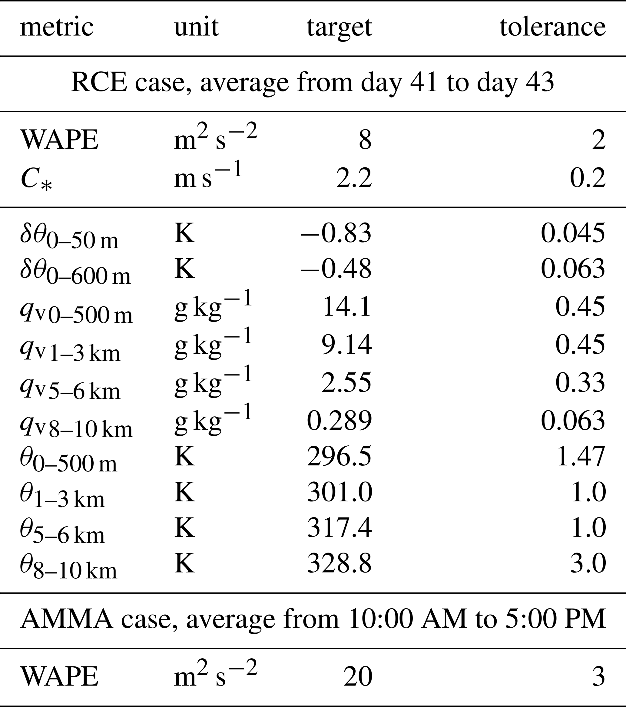
Table A2Free parameters considered in the tuning exercise, along with their values in the control simulation (initial values) and in the BEST TUNE simulation.
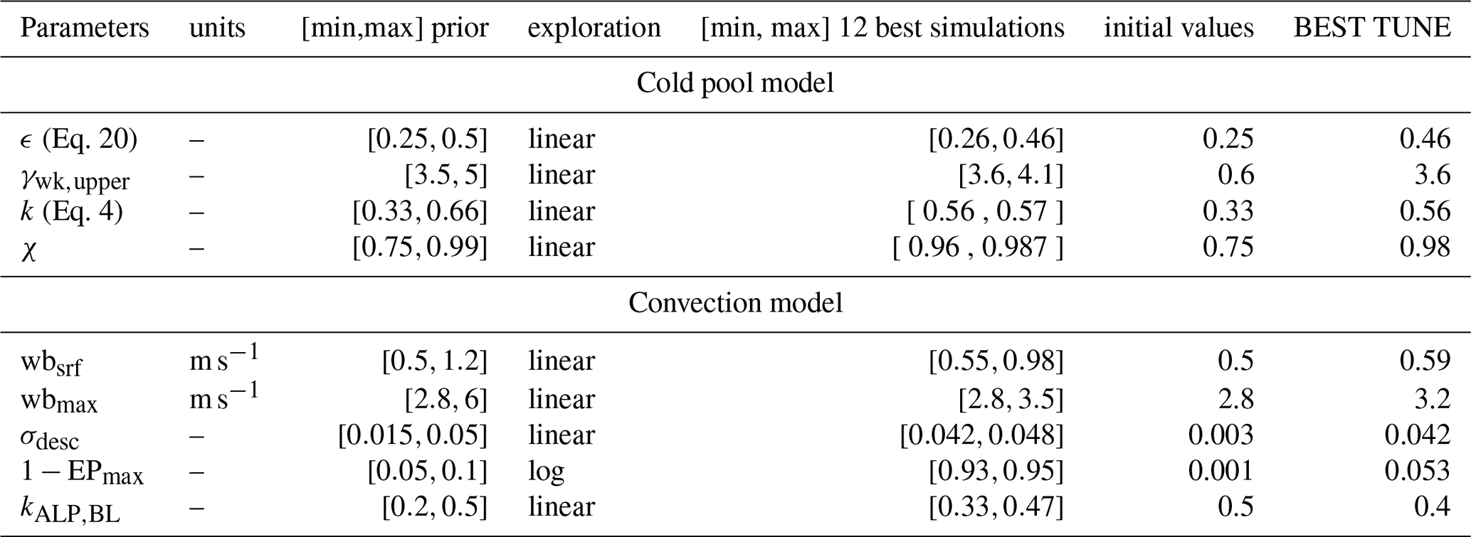
The codes used are distributed openly through subversion. The LMDZ GCM is available at: http://svn.lmd.jussieu.fr/LMDZ/LMDZ6/trunk (last access: 28 February 2025). It can be installed automatically on a laptop with the command http://lmdz.lmd.jussieu.fr/pub/install_lmdz.sh (last access: 28 February 2025). The htexplo tool is available at: https://svn.lmd.jussieu.fr/HighTune/trunk (last access: 10 September 2025). The data and scripts used in this study are available at the following DOI: https://doi.org/10.5281/zenodo.20548562 (Thiam et al., 2026).
Mamadou Lamine Thiam: work design, diagnostics, analysis, figures and writing. Frédéric Hourdin: work design, diagnostics, analysis and writing. Jean-Yves Grandpeix: conception of the work, analysis and writing. Catherine Rio: RCE simulation with Meso-NH, analysis and writing. Maëlle Coulon–Decorzens: tuning expertise.
The contact author has declared that none of the authors has any competing interests.
Publisher's note: Copernicus Publications remains neutral with regard to jurisdictional claims made in the text, published maps, institutional affiliations, or any other geographical representation in this paper. The authors bear the ultimate responsibility for providing appropriate place names. Views expressed in the text are those of the authors and do not necessarily reflect the views of the publisher.
The authors thank Caroline Müller for providing the RCE simulation run with the SAM model and Fleur Couvreux for providing the AMMA simulation run with the Meso-NH model. We also acknowledge support from the DEPHY research group of CLIMERI, funded by CNRS/INSU and Météo-France. It benefited from the development of the htexplo tool within this project and automation of LES/SCM simulations through standardization of IO formats.
Mamadou Lamine Thiam's doctoral thesis was supported by Institute de Recherche pour le Développement (IRD) as part of the international doctoral program entitled “Modélisation des Systèmes Complexes” (PDI-MSC). The thesis also received financial support from the Cuomo Foundation (Monaco) as part of an IPCC support program. This study has received funding from Agence Nationale de la Recherche – France 2030 as part of the PEPR TRACCS programme under grant number ANR-22-EXTR-0008. This study also recieved a funding from the French Agence Nationale de la Recherche under grant no. ANR-21-CE46-0013 (Monte Carlo Simulations for Meteorology and Climatology project).
This paper was edited by Johannes Quaas and reviewed by two anonymous referees.
Böing, S. J., Jonker, H. J. J., Siebesma, A. P., and Grabowski, W. W.: Influence of the subcloud layer on the development of a deep convective ensemble, J. Atmos. Sci., 69, 2682–2698, https://doi.org/10.1175/JAS-D-11-0317.1, 2012. a
Boucher, O., Denvil, S., Levavasseur, G., Cozic, A., Caubel, A., Foujols, M.-A., Meurdesoif, Y., Balkanski, Y., Checa-Garcia, R., Hauglustaine, D., Bekki, S., and Marchand, M.: IPSL IPSL-CM6A-LR-INCA model output prepared for CMIP6 RFMIP piClim-aer, Earth System Grid Federation [data set], https://doi.org/10.22033/ESGF/CMIP6.14604, 2020. a
Brown, A. R., Cederwall, R. T., Chlond, A., Duynkerke, P. G., Golaz, J.-C., Khairoutdinov, M., Lewellen, D. C., Lock, A. P., MacVean, M. K., Moeng, C.-H., Neggers, R. A. J., Siebesma, A. P., and Stevens, B.: Large-eddy simulation of the diurnal cycle of shallow cumulus convection over land, Q. J. Roy. Meteor. Soc., 128, 1075–1093, https://doi.org/10.1256/003590002320373210, 2002. a, b
Bryan, G. H.: Spurious convective organization in simulated squall lines owing to moist absolutely unstable layers, Mon. Weather Rev., 133, 1978–1997, https://doi.org/10.1175/MWR2952.1, 2005. a
Charba, J.: Application of gravity current model to analysis of squall-line gust front, Mon. Weather Rev., 102, 140–156, https://doi.org/10.1175/1520-0493(1974)102<0140:AOGCMT>2.0.CO;2, 1974. a
Chatfield, R. B. and Brost, R. A.: A two-stream model of the vertical transport of trace species in the convective boundary layer, J. Geophys. Res.-Atmos., 92, 13263–13276, https://doi.org/10.1029/JD092iD11p13263, 1987. a
Couvreux, F., Rio, C., Guichard, F., Lothon, M., Canut, G., Bouniol, D., and Gounou, A.: Initiation of daytime local convection in a semi-arid region analysed with high-resolution simulations and AMMA observations, Q. J. Roy. Meteor. Soc., 138, 56–71, https://doi.org/10.1002/qj.903, 2012. a
Couvreux, F., Hourdin, F., Williamson, D., Roehrig, R., Volodina, V., Villefranque, N., Rio, C., Audouin, O., Salter, J., Bazile, E., Brient, F., Favot, F., Honnert, R., Lefebvre, M.-P., Madeleine, J.-B., Rodier, Q., and Xu, W.: Process-based climate model development harnessing machine learning: I. A calibration tool for parameterization improvement, J. Adv. Model. Earth Sy., 13, e2020MS002217, https://doi.org/10.1029/2020MS002217, 2021. a, b, c, d
Daleu, C. L., Plant, R. S., Woolnough, S. J., Sessions, S., Herman, M. J., Sobel, A., Wang, S., Kim, D., Cheng, A., Bellon, G., Peyrille, P., Ferry, F., Siebesma, P., and van Ulft, L.: Intercomparison of methods of coupling between convection and large-scale circulation: 1. Comparison over uniform surface conditions, J. Adv. Model. Earth Sy., 7, 1576–1601, https://doi.org/10.1002/2015MS000468, 2015. a
Del Genio, A. D., Wu, J., Wolf, A. B., Chen, Y., Yao, M.-S., and Kim, D.: Constraints on cumulus parameterization from simulations of observed MJO events, J. Climate, 28, 6419–6442, https://doi.org/10.1175/JCLI-D-14-00832.1, 2015. a, b
Diallo, F. B., Hourdin, F., Rio, C., Traore, A.-K., Mellul, L., Guichard, F., and Kergoat, L.: The surface energy budget computed at the grid-scale of a climate model challenged by station data in West Africa, J. Adv. Model. Earth Sy., 9, 2710–2738, https://doi.org/10.1002/2017MS001081, 2017. a, b
Dirmeyer, P. A., Cash, B. A., Kinter, J. L., Jung, T., Marx, L., Satoh, M., Stan, C., Tomita, H., Towers, P., Wedi, N., Achuthavarier, D., Adams, J. M., Altshuler, E. L., Huang, B., Jin, E. K., and Manganello, J.: Simulating the diurnal cycle of rainfall in global climate models: Resolution versus parameterization, Clim. Dynam., 39, 399–418, https://doi.org/10.1007/s00382-011-1127-9, 2012. a
Dorrestijn, J., Crommelin, D. T., Siebesma, A. P., and Jonker, H. J. J.: Stochastic parameterization of shallow cumulus convection estimated from high-resolution model data, Theor. Comp. Fluid Dyn., 27, 133–148, https://doi.org/10.1007/s00162-012-0281-y, 2013. a
Droegemeier, K. K. and Wilhelmson, R. B.: Numerical simulation of thunderstorm outflow dynamics. Part I: Outflow sensitivity experiments and turbulence dynamics, J. Atmos. Sci., 44, 1180–1210, https://doi.org/10.1175/1520-0469(1987)044<1180:NSOTOD>2.0.CO;2, 1987. a
Emanuel, K. A.: A scheme for representing cumulus convection in large-scale models, J. Atmos. Sci., 48, 2313–2335, https://doi.org/10.1175/1520-0469(1991)048<2313:ASFRCC>2.0.CO;2, 1991. a, b, c
Feng, Z., Hagos, S., Rowe, A. K., Burleyson, C. D., Martini, M. N., and de Szoeke, S. P.: Mechanisms of convective cloud organization by cold pools over tropical warm ocean during the AMIE/DYNAMO field campaign, J. Adv. Model. Earth Sy., 7, 357–381, https://doi.org/10.1002/2014MS000384, 2015. a, b
Freitas, S. R., Grell, G. A., Chovert, A. D., Silva Dias, M. A. F., and de Lima Nascimento, E.: A parameterization for cloud organization and propagation by evaporation-driven cold pool edges, J. Adv. Model. Earth Sy., 16, e2023MS003982, https://doi.org/10.1029/2023MS003982, 2024. a, b, c, d
Gettelman, A., Truesdale, J. E., Bacmeister, J. T., Caldwell, P. M., Neale, R. B., Bogenschutz, P. A., and Simpson, I. R.: The Single Column Atmosphere Model version 6 (SCAM6): Not a scam but a tool for model evaluation and development, J. Adv. Model. Earth Sy., 11, 1381–1401, https://doi.org/10.1029/2018MS001578, 2019. a
Grandpeix, J.-Y. and Lafore, J.-P.: A density current parameterization coupled with Emanuel's convection scheme. Part I: The models, J. Atmos. Sci., 67, 881–897, https://doi.org/10.1175/2009JAS3044.1, 2010. a, b, c, d, e, f
Grandpeix, J.-Y., Phillips, V., and Tailleux, R.: Improved mixing representation in Emanuel's convection scheme, Quarterly Journal of the Royal Meteorological Society: A journal of the atmospheric sciences, Applied Meteorology and Physical Oceanography, 130, 3207–3222, https://doi.org/10.1256/qj.03.144, 2004. a
Grandpeix, J.-Y., Lafore, J.-P., and Cheruy, F.: A density current parameterization coupled with Emanuel's convection scheme. Part II: 1D simulations, J. Atmos. Sci., 67, 898–922, https://doi.org/10.1175/2009JAS3045.1, 2010. a, b
Grant, L. D., Lane, T. P., and van den Heever, S. C.: The role of cold pools in tropical oceanic convective systems, J. Atmos. Sci., 75, 2615–2634, https://doi.org/10.1175/JAS-D-17-0352.1, 2018. a
Guichard, F., Petch, J. C., Redelsperger, J.-L., Bechtold, P., Chaboureau, J.-P., Cheinet, S., Grabowski, W., Grenier, H., Jones, C. G., Köhler, M., Piriou, J.-M., Tailleux, R., and Tomasini, M.: Modelling the diurnal cycle of deep precipitating convection over land with cloud-resolving models and single-column models, Q. J. Roy. Meteor. Soc., 130, 3139–3172, https://doi.org/10.1002/qj.503, 2004. a
Haerter, J. O. and Schlemmer, L.: Intensified cold pool dynamics under stronger surface heating, Geophys. Res. Lett., 45, 6299–6310, https://doi.org/10.1029/2017GL076874, 2018. a
Hourdin, F., Couvreux, F., and Menut, L.: Parameterization of the Dry Convective Boundary Layer Based on a Mass Flux Representation of Thermals, J. Atmos. Sci., 59, 1105–1123, https://doi.org/10.1175/1520-0469(2002)059<1105:POTDCB>2.0.CO;2, 2002. a
Hourdin, F., Musat, I., Bony, S., Braconnot, P., Codron, F., Dufresne, J.-L., Fairhead, L., Filiberti, M.-A., Friedlingstein, P., Grandpeix, J.-Y., Krinner, G., LeVan, P., Li, Z.-X., and Lott, F.: The LMDZ4 general circulation model: climate performance and sensitivity to parametrized physics with emphasis on tropical convection, Clim. Dynam., 27, 787–813, https://doi.org/10.1007/s00382-006-0158-0, 2006. a
Hourdin, F., Foujols, M.-A., Codron, F., Guemas, V., Dufresne, J.-L., Bony, S., Denvil, S., Guez, L., Lott, F., Ghattas, J., Braconnot, P., Marti, O., Meurdesoif, Y., and Bopp, L.: Impact of the LMDZ atmospheric grid configuration on the climate and sensitivity of the IPSL-CM5A coupled model, Clim. Dynam., 40, 2167–2192, https://doi.org/10.1007/s00382-012-1411-3, 2013. a
Hourdin, F., Jam, A., Rio, C., Couvreux, F., Sandu, I., Lefebvre, M.-P., Brient, F., and Idelkadi, A.: Unified Parameterization of Convective Boundary Layer Transport and Clouds With the Thermal Plume Model, J. Adv. Model. Earth Sy., 11, 2910–2933, https://doi.org/10.1029/2019MS001666, 2019. a
Hourdin, F., Rio, C., Grandpeix, J.-Y., Madeleine, J.-B., Cheruy, F., Rochetin, N., Jam, A., Musat, I., Idelkadi, A., Fairhead, L., Foujols, M.-A., Mellul, L., Traore, A.-K., Dufresne, J.-L., Boucher, O., Lefebvre, M.-P., Millour, E., Vignon, E., Jouhaud, J., and Diallo, F. B.: LMDZ6A: The atmospheric component of the IPSL climate model with improved and better tuned physics, J. Adv. Model. Earth Sy., 12, e2019MS001892, https://doi.org/10.1029/2019MS001892, 2020a. a, b
Hourdin, F., Rio, C., Jam, A., Traore, A.-K., and Musat, I.: Convective Boundary Layer Control of the Sea Surface Temperature in the Tropics, J. Adv. Model. Earth Sy., 12, e01988, https://doi.org/10.1029/2019MS001988, 2020b. a
Hourdin, F., Williamson, D., Rio, C., Couvreux, F., Roehrig, R., Villefranque, N., Musat, I., Fairhead, L., Diallo, F. B., and Volodina, V.: Process-based climate model development harnessing machine learning: II. Model calibration from single column to global, J. Adv. Model. Earth Sy., 13, e2020MS002 225, https://doi.org/10.1029/2020MS002225, 2021. a, b, c
Jam, A., Hourdin, F., Rio, C., and Couvreux, F.: Resolved Versus Parametrized Boundary-Layer Plumes. Part III: Derivation of a Statistical Scheme for Cumulus Clouds, Bound.-Lay. Meteorol., 147, 421–441, https://doi.org/10.1007/s10546-012-9789-3, 2013. a
Jeevanjee, N. and Romps, D. M.: Convective self-aggregation, cold pools, and domain size, Geophys. Res. Lett., 40, 994–998, https://doi.org/10.1002/grl.50204, 2013. a
Kendon, E. J., Roberts, N. M., Senior, C. A., and Roberts, M. J.: Realism of rainfall in a very high-resolution regional climate model, J. Climate, 25, 5791–5806, https://doi.org/10.1175/JCLI-D-11-00562.1, 2012. a
Khairoutdinov, M. and Randall, D.: High-resolution simulation of shallow-to-deep convection transition over land, J. Atmos. Sci., 63, 3421–3436, https://doi.org/10.1175/JAS3810.1, 2006. a
Khairoutdinov, M. F. and Randall, D. A.: Cloud resolving modeling of the ARM summer 1997 IOP: Model formulation, results, uncertainties, and sensitivities, J. Atmos. Sci., 60, 607–625, https://doi.org/10.1175/1520-0469(2003)060<0607:CRMOTA>2.0.CO;2, 2003. a
Krueger, S. K., Morrison, H., and Fridlind, A. M.: Cloud-resolving modeling: ARM and the GCSS story, Meteor. Mon., 57, 25.1–25.16, https://doi.org/10.1175/AMSMONOGRAPHS-D-15-0047.1, 2016. a
Kurowski, M. J., Suselj, K., Grabowski, W. W., and Teixeira, J.: Shallow-to-deep transition of continental moist convection: Cold pools, surface fluxes, and mesoscale organization, J. Atmos. Sci., 75, 4071–4090, https://doi.org/10.1175/JAS-D-18-0031.1, 2018. a
Lac, C., Chaboureau, J.-P., Masson, V., Pinty, J.-P., Tulet, P., Escobar, J., Leriche, M., Barthe, C., Aouizerats, B., Augros, C., Aumond, P., Auguste, F., Bechtold, P., Berthet, S., Bielli, S., Bosseur, F., Caumont, O., Cohard, J.-M., Colin, J., Couvreux, F., Cuxart, J., Delautier, G., Dauhut, T., Ducrocq, V., Filippi, J.-B., Gazen, D., Geoffroy, O., Gheusi, F., Honnert, R., Lafore, J.-P., Lebeaupin Brossier, C., Libois, Q., Lunet, T., Mari, C., Maric, T., Mascart, P., Mogé, M., Molinié, G., Nuissier, O., Pantillon, F., Peyrillé, P., Pergaud, J., Perraud, E., Pianezze, J., Redelsperger, J.-L., Ricard, D., Richard, E., Riette, S., Rodier, Q., Schoetter, R., Seyfried, L., Stein, J., Suhre, K., Taufour, M., Thouron, O., Turner, S., Verrelle, A., Vié, B., Visentin, F., Vionnet, V., and Wautelet, P.: Overview of the Meso-NH model version 5.4 and its applications, Geosci. Model Dev., 11, 1929–1969, https://doi.org/10.5194/gmd-11-1929-2018, 2018. a
Lafore, J.-P. and Moncrieff, M. W.: A numerical investigation of the organization and interaction of the convective and stratiform regions of tropical squall lines, J. Atmos. Sci., 46, 521–544, https://doi.org/10.1175/1520-0469(1989)046<0521:ANIOTO>2.0.CO;2, 1989. a
Legay, A., Deremble, B., and Burchard, H.: Derivation and implementation of a non-local term to improve the oceanic convection representation within the k–ϵ parameterization, J. Adv. Model. Earth Sy., 17, e2024MS004243, https://doi.org/10.1029/2024MS004243, 2025. a
Lochbihler, K., Lenderink, G., and Siebesma, A. P.: Cold pool dynamics shape the response of extreme rainfall events to climate change, J. Adv. Model. Earth Sy., 13, e2020MS002306, https://doi.org/10.1029/2020MS002306, 2021. a
Lothon, M., Campistron, B., Chong, M., Couvreux, F., Guichard, F., Rio, C., and Williams, E.: Life cycle of a mesoscale circular gust front observed by a C-band Doppler radar in West Africa, Mon. Weather Rev., 139, 1370–1388, https://doi.org/10.1175/2010MWR3480.1, 2011. a, b
Ma, H.-Y., Chuang, C. C., Klein, S. A., Lo, M.-H., Zhang, Y., Xie, S., Zheng, X., Ma, P.-L., Zhang, Y., and Phillips, T. J.: An improved hindcast approach for evaluation and diagnosis of physical processes in global climate models, J. Adv. Model. Earth Sy., 7, 1810–1827, https://doi.org/10.1002/2015MS000490, 2015. a
Meyer, B. and Haerter, J. O.: Mechanical forcing of convection by cold pools: Collisions and energy scaling, J. Adv. Model. Earth Sy., 12, e2020MS002 281, https://doi.org/10.1029/2020MS002281, 2020. a, b
Pantillon, F., Knippertz, P., Marsham, J. H., and Birch, C. E.: A parameterization of convective dust storms for models with mass-flux convection schemes, J. Atmos. Sci., 72, 2545–2561, https://doi.org/10.1175/JAS-D-14-0341.1, 2015. a, b
Park, S.: A unified convection scheme (UNICON). Part I: Formulation, J. Atmos. Sci., 71, 3902–3930, https://doi.org/10.1175/JAS-D-13-0233.1, 2014. a, b, c
Park, S., Song, C., Kim, S., and Kim, J.: Parameterization of the elevated convection with a unified convection scheme (UNICON) and its impacts on the diurnal cycle of precipitation, J. Adv. Model. Earth Sy., 16, e2023MS003651, https://doi.org/10.1029/2023MS003651, 2024. a
Piriou, J.-M., Redelsperger, J.-L., Geleyn, J.-F., Lafore, J.-P., and Guichard, F.: An approach for convective parameterization with memory: Separating microphysics and transport in grid-scale equations, J. Atmos. Sci., 64, 4127–4139, https://doi.org/10.1175/2007JAS2144.1, 2007. a, b
Provod, M., Marsham, J. H., Parker, D. J., and Birch, C. E.: A characterization of cold pools in the West African Sahel, Mon. Weather Rev., 144, 1923–1934, https://doi.org/10.1175/MWR-D-15-0023.1, 2016. a
Qian, L., Young, G. S., and Frank, W. M.: A convective wake parameterization scheme for use in general circulation models, Mon. Weather Rev., 126, 456–469, https://doi.org/10.1175/1520-0493(1998)126<0456:ACWPSF>2.0.CO;2, 1998. a
Randall, D., Khairoutdinov, M., Arakawa, A., and Grabowski, W.: Breaking the cloud parameterization deadlock, B. Am. Meteorol. Soc., 84, 1547–1564, https://doi.org/10.1175/BAMS-84-11-1547, 2003. a, b
Redelsperger, J.-L., Diedhiou, A., Flamant, C., Janicot, S., Lafore, J.-P., Lebel, T., Polcher, J., Bourlès, B., Caniaux, G., de Rosnay, P., Desbois, M., Eymard, L., Fontaine, B., Geneau, I., Ginoux, K., Hoepffner, M., Kane, C., Law, K., Mari, C., Marticorena, B., Mougin, E., Pelon, J., Peugeot, C., Protat, A., Roux, F., Sultan, B., and Van Den Akker, E.: Amma, une étude multidisciplinaire de la mousson ouest-africaine, La Météorologie, 54, 22–32, https://doi.org/10.4267/2042/20098, 2006. a
Rio, C. and Hourdin, F.: A thermal plume model for the convective boundary layer: Representation of cumulus clouds, J. Atmos. Sci., 65, 407–425, https://doi.org/10.1175/2007JAS2256.1, 2008. a, b
Rio, C., Hourdin, F., Grandpeix, J.-Y., and Lafore, J.-P.: Shifting the diurnal cycle of parameterized deep convection over land, Geophys. Res. Lett., 36, https://doi.org/10.1029/2008GL036779, 2009. a, b, c, d, e
Rio, C., Grandpeix, J.-Y., Hourdin, F., Guichard, F., Couvreux, F., Lafore, J.-P., Fridlind, A., Mrowiec, A., Bony, S., Rochetin, N., Roehrig, R., Idelkadi, A., Lefebvre, M.-P., and Musat, I.: Control of deep convection by sub-cloud lifting processes: the ALP closure in the LMDZ5B general circulation model, Clim. Dynam., 40, 2271–2292, https://doi.org/10.1007/s00382-012-1506-x, 2013. a
Rochetin, N., Grandpeix, J.-Y., Rio, C., and Couvreux, F.: Deep convection triggering by boundary layer thermals. Part II: Stochastic triggering parameterization for the LMDZ GCM, J. Atmos. Sci., 71, 515–538, https://doi.org/10.1175/JAS-D-12-0337.1, 2014. a, b
Rochetin, N., Hohenegger, C., Touzé-Peiffer, L., and Villefranque, N.: A physically based definition of convectively generated density currents: Detection and characterization in convection-permitting simulations, J. Adv. Model. Earth Sy., 13, e2020MS002402, https://doi.org/10.1029/2020MS002402, 2021. a, b
Rooney, G. G., Stirling, A. J., Stratton, R. A., and Whitall, M.: C-POOL: A scheme for modelling convective cold pools in the Met Office Unified Model, Q. J. Roy. Meteor. Soc., 148, 962–980, https://doi.org/10.1002/qj.4241, 2022. a, b, c, d, e, f
Rotunno, R., Klemp, J. B., and Weisman, M. L.: A theory for strong, long-lived squall lines, J. Atmos. Sci., 45, 463–485, https://doi.org/10.1175/1520-0469(1988)045<0463:ATFSLL>2.0.CO;2, 1988. a
Sadourny, R. and Laval, K.: January and July performances of the LMD general circulation model, in: New Perspectives in Climate Modelling, edited by: Berger, A. and Nicolis, C., Elsevier, 173–197, ISBN 978-0444422958, 1984. a, b
Siebesma, A. P., Bretherton, C. S., Brown, A., Chlond, A., Cuxart, J., Duynkerke, P. G., Jiang, H., Khairoutdinov, M., Lewellen, D., Moeng, C.-H., Sanchez, E., Stevens, B., and Stevens, D. E.: A large eddy simulation intercomparison study of shallow cumulus convection, J. Atmos. Sci., 60, 1201–1219, https://doi.org/10.1175/1520-0469(2003)60<1201:ALESIS>2.0.CO;2, 2003. a, b
Stephens, G. L., L'Ecuyer, T., Forbes, R., Gettelmen, A., Golaz, J.-C., Bodas-Salcedo, A., Suzuki, K., Gabriel, P., and Haynes, J.: Dreary state of precipitation in global models, J. Geophys. Res.-Atmos., 115, D24211, https://doi.org/10.1029/2010JD014532, 2010. a
Strauss, C., Ricard, D., Lac, C., and Verrelle, A.: Evaluation of turbulence parametrizations in convective clouds and their environment based on a large-eddy simulation, Q. J. Roy. Meteor. Soc., 145, 3195–3217, https://doi.org/10.1002/qj.3605, 2019. a
Suselj, K., Kurowski, M. J., and Teixeira, J.: A unified eddy-diffusivity/mass-flux approach for modeling atmospheric convection, J. Atmos. Sci., 76, 2505–2537, https://doi.org/10.1175/JAS-D-18-0239.1, 2019. a, b, c, d, e
Tan, J., Oreopoulos, L., Jakob, C., and Jin, D.: Evaluating rainfall errors in global climate models through cloud regimes, Clim. Dynam., 50, 3301–3314, https://doi.org/10.1007/s00382-017-3806-7, 2018. a
Thiam, M. L., Hourdin, F., Grandpeix, J.-Y., Rio, C., and Coulon-Decorzens, M.: Data and scripts used in the study: Evaluation and improvement of the cold pool parameterization in the LMDZ climate model against Large Eddy Simulations, Zenodo [data set], https://doi.org/10.5281/zenodo.20548562, 2026. a
Torri, G. and Kuang, Z.: On cold pool collisions in tropical boundary layers, Geophys. Res. Lett., 46, 399–407, https://doi.org/10.1029/2018GL080501, 2019. a
Touzé-Peiffer, L., Vogel, R., and Rochetin, N.: Cold pools observed during eurec 4 a: Detection and characterization from atmospheric soundings, J. Appl. Meteorol. Clim., 61, 593–610, https://doi.org/10.1175/JAMC-D-21-0048.1, 2022. a
Vogel, R., Konow, H., Schulz, H., and Zuidema, P.: A climatology of trade-wind cumulus cold pools and their link to mesoscale cloud organization, Atmos. Chem. Phys., 21, 16609–16630, https://doi.org/10.5194/acp-21-16609-2021, 2021. a
Weisman, M. L. and Rotunno, R.: “A theory for strong long-lived squall lines” revisited, J. Atmos. Sci., 61, 361–382, https://doi.org/10.1175/1520-0469(2004)061<0361:ATFSLS>2.0.CO;2, 2004. a
Williamson, D., Goldstein, M., Allison, L., Blaker, A., Challenor, P., Jackson, L., and Yamazaki, K.: History matching for exploring and reducing climate model parameter space using observations and a large perturbed physics ensemble, Clim. Dynam., 41, 1703–1729, https://doi.org/10.1007/s00382-013-1896-4, 2013. a
Wing, A. A., Reed, K. A., Satoh, M., Stevens, B., Bony, S., and Ohno, T.: Radiative–convective equilibrium model intercomparison project, Geosci. Model Dev., 11, 793–813, https://doi.org/10.5194/gmd-11-793-2018, 2018. a
Yamada, T.: Simulations of Nocturnal Drainage Flows by a q2l Turbulence Closure Model, J. Atmos. Sci., 40, 91–106, https://doi.org/10.1175/1520-0469(1983)040<0091:SONDFB>2.0.CO;2, 1983. a
Yanai, M., Esbensen, S., and Chu, J.-H.: Determination of bulk properties of tropical cloud clusters from large-scale heat and moisture budgets, J. Atmos. Sci., 30, 611–627, https://doi.org/10.1175/1520-0469(1973)030<0611:DOBPOT>2.0.CO;2, 1973. a
Young, G. S., Perugini, S. M., and Fairall, C. W.: Convective wakes in the equatorial western Pacific during TOGA, Mon. Weather Rev., 123, 110–123, https://doi.org/10.1175/1520-0493(1995)123<0110:CWITEW>2.0.CO;2, 1995. a
Zhang, M., Somerville, R. C. J., and Xie, S.: The SCM concept and creation of ARM forcing datasets, Meteor. Mon., 57, 24.1–24.12, https://doi.org/10.1175/AMSMONOGRAPHS-D-15-0040.1, 2016. a
Zuidema, P., Torri, G., Muller, C., and Chandra, A.: A survey of precipitation-induced atmospheric cold pools over oceans and their interactions with the larger-scale environment, Surv. Geophys., 38, 1283–1305, https://doi.org/10.1007/s10712-017-9447-x, 2017. a
- Abstract
- Introduction
- Tools and methods
- Assessment of the cold pool model internal equations from LES
- Evaluation in the single column configuration of LMDZ
- Improvements of the cold pool model
- Conclusions
-
Appendix A:
htexploand the tuning setup - Code and data availability
- Author contributions
- Competing interests
- Disclaimer
- Acknowledgements
- Financial support
- Review statement
- References
- Abstract
- Introduction
- Tools and methods
- Assessment of the cold pool model internal equations from LES
- Evaluation in the single column configuration of LMDZ
- Improvements of the cold pool model
- Conclusions
-
Appendix A:
htexploand the tuning setup - Code and data availability
- Author contributions
- Competing interests
- Disclaimer
- Acknowledgements
- Financial support
- Review statement
- References