A localized plant species-specific BVOC emission rate library of China established using a developed statistical approach based on field measurements

Precise quantification of biogenic volatile organic compound (BVOC) emissions is essential for effective control of ozone and secondary organic aerosol pollution. However, the lack of a localized and detailed plant species–specific emission rate library poses significant challenges to accurate emission estimates in China. Additionally, large uncertainty exists in the representative emission rates used in inventory compilation. Here, a statistical approach for classifying emission intensity and assigning representative emission rates with higher accuracy was developed from our measurements and local field observations. Furthermore, a localized plant species–specific BVOC emission rate library for China covering 599 plant species was established. Critically, different reliability levels were assigned to each emission rate according to the measurement technique. Emission simulations were conducted to evaluate the implications of the developed library. Comparison with formaldehyde vertical column density observations showed that our localized library improved the model performance in capturing the spatial variations of isoprene emissions. The newly estimated BVOC emissions were 27.70 Tg, 18 % higher than estimates based on the global library. Updating the localized emission rates reduced underestimation in southern and overestimation in northeast and western China.

1 Introduction

Biogenic volatile organic compounds (BVOCs) are primarily emitted by vegetation in terrestrial ecosystems (Ciccioli et al., 2023; Guenther et al., 1995, 2012; Li et al., 2023, 2024; Simpson et al., 1999). These compounds are highly reactive (Atkinson and Arey, 2003), which can react with nitrogen oxides (NO_x) to generate ozone (O₃) and secondary organic aerosol (SOA) through atmospheric oxidation (Li et al., 2022; Wei et al., 2024), thereby affecting air quality, cloud formation, solar radiation transmission, and climate change (Blichner et al., 2024; Ndah et al., 2024). Furthermore, the O₃ formation can be more sensitive to BVOCs than to NO_x in VOC-limited areas (Guo et al., 2024; Huang et al., 2024; Wang et al., 2023a). In China, both the reduction of anthropogenic VOCs and the growth of BVOC emissions in recent years (Cao et al., 2024a; Gai et al., 2024) have enhanced the contribution of BVOCs to O₃ and SOA formation (Yang et al., 2023). Cao et al. (2022) reported that summertime BVOC emissions led to an average increase of 8.6 ppb (17 %) in daily maximum 8 h (MDA8) O₃ concentration and 0.84 µg m⁻³ (73 %) in SOA over China. Accurately estimating BVOC emissions is essential for the precise control of complex air pollution in China.

Reported BVOC emission inventories for China have shown variable results and large uncertainties (Li et al., 2024). The quality of emission rates in an inventory substantially influences the accuracy of emission estimates (Wang et al., 2023b). In existing inventories, different emission rates have been applied to the same plant species due to variations in assignment methods. Mostly, global emission rates by plant function type (PFT) were used, although these include a few observations from China. Emissions from domestic and foreign plants often differ due to genetic, environmental, and climatic factors (Chatani et al., 2018). Uncertainties will inevitably be introduced when foreign measurements are used in Chinese emission inventories. Therefore, it is essential to localize the emission rate library. Some inventories used limited local observations, but large uncertainties remained. In some cases, the emission rate was assigned based on a single observation or by directly averaging multiple observations. This approach introduces uncertainties because local measurements are limited and different studies may report varying emission rates for the same plant species (Chen et al., 2024; Zeng et al., 2024). Subsequently, some studies applied a method based on emission intensity categories to determine the emission rates used in inventory compilation (Klinger et al., 2002; Wang et al., 2007; Yan et al., 2005). In this method, different emission intensity categories (e.g., negligible, low, moderate, and high) are defined, each with a representative emission rate and a range of ±50 % (Simpson et al., 1999; Zhang et al., 2024). For each plant species, the emission rate is determined from the tendency of reported values to fall within certain categories. This method can substantially improve the accuracy of final emission rates; however, it has several limitations. First, the process of determining emission categories, representative emission rates, and ranges is not straightforward and lacks theoretical justification. Second, the various emission categories and representative values in different studies have led to disparate emission rates for the same plant species. For example, Klinger et al. (2002) assigned isoprene emission rates of 70, 70, and 14 $\mathrm{\mu }\mathrm{g}\mathrm{C}{\mathrm{g}}^{-\mathrm{1}}{\mathrm{h}}^{-\mathrm{1}}$ for Saliix character, Quercus mongolica, and Picea jezoensis, respectively, whereas Wang et al. (2007) reported values of 20, 50, and 10 $\mathrm{\mu }\mathrm{g}\mathrm{C}{\mathrm{g}}^{-\mathrm{1}}{\mathrm{h}}^{-\mathrm{1}}$. Third, most studies used coarse classifications of emission, typically five to seven categories (Klinger et al., 2002; Yan et al., 2005), which may result in imprecise classifications and overestimation or underestimation of emission rates for specific plant species. Significant uncertainties will be further introduced into BVOC emission estimates. Thus, detailed emission categories and accurate representative values and ranges are essential for accurately estimating emission rates. Additionally, a localized BVOC emission rate library should be established based on domestic observations to enhance inventory accuracy. Additionally, PFT-averaged emission rates were often used, which fail to capture the species specificity of BVOC emissions. Research has shown that isoprene emission rates can vary by 220 %–330 % among vegetation subtypes (Batista et al., 2019). Therefore, it is also necessary to establish a plant species–specific emission rate library.

In this study, we first conducted the emission measurements for plants in China to provide more baseline data for the establishment of a localized emission rate library. Second, by summarizing our field measurements along with reported emission rates from China, we developed a statistical approach to determine plant species–specific emission rates. A localized BVOC emission rate library for China was established, and its features were analyzed. Differences in BVOC emission rates among vegetation types, families, genera, and species were examined. Then, the developed emission rate library was applied to establish a BVOC emission inventory for China using the Model of Emissions of Gases and Aerosols from Nature (MEGAN) v3.2. Its performance was further evaluated. Furthermore, the influence of emission rates with different reliability levels on the estimated BVOC emission was investigated. This study will be significant for improving the accuracy of local biogenic emission inventories and, in turn, air quality modeling. Additionally, our developed statistical approach can be extended to the establishment of BVOC emission rate libraries for other regions.

2 Field measurements of emission rates

Field measurements of BVOC emission rates were conducted from July 2020–September 2023. The sites covered the south and north of China, including Shandong, Hebei, Jiangsu, and Anhui Provinces. Their specific locations are shown in Fig. S1 in the Supplement. Meanwhile, some pot experiments in the plant growth chamber were included. Emissions from 66 plant species – including 30 broadleaf trees, 12 coniferous trees, 20 shrubs, two crops, and two herb species – were measured (Table S1 in the Supplement). The dynamic enclosure technique was used for the observations, as depicted in Fig. 1 (Zhang et al., 2024). First, selected branches were enclosed within a Teflon bag (Welch Fluorocarbon, Inc., USA) with a volume ranging from 15–60 L and a PAR transparency close to 100 %. The bag was made of polytetrafluoroethylene, a material known for its inherent chemical inertness that minimizes the generation and adsorption of VOCs without requiring additional treatment (Zhang et al., 2024). Clean air was continuously introduced into the bag at a constant flow rate of 10–20 L min⁻¹ after removing water, O₃, and VOCs through silicone rubber, potassium iodide, and activated carbon. After equilibrium, the gases in the bag were collected into adsorption tubes filled with Tenax TA and Carbograph 5TD (Markes International, Bridgend, UK) using an air-sampling pump (Gilian Gilair Plus, Sensidyne, USA) with a flow rate of 200 mL min⁻¹ for 30 min. For each plant species, three mature and healthy individuals were selected as replicates, and one blank sample was used as the background. During the whole enclosure, the temperature and photosynthetically active radiation (PAR) were recorded in real time. After the experiment, all leaves on the enclosed branch were collected and weighed after drying at 75 °C for 48 h.

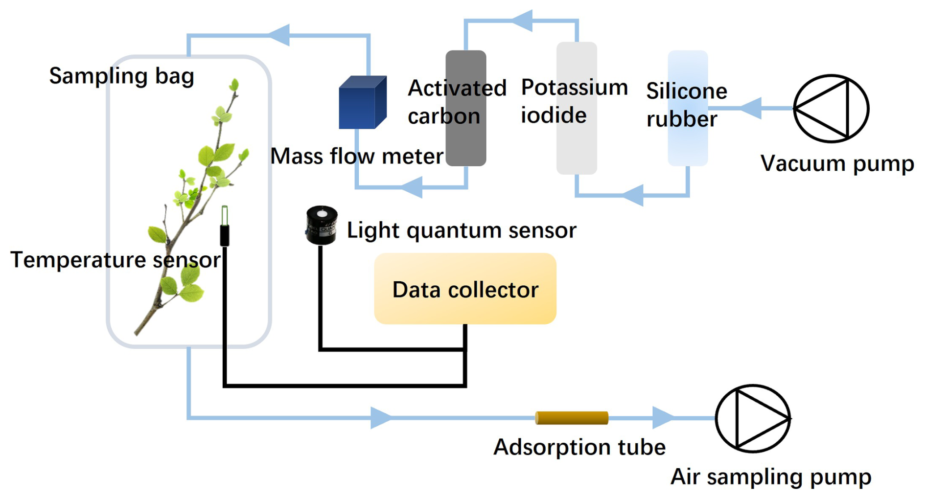
Figure 1 Schematic of dynamic enclosure technique. Vacuum pump was used to introduce air to the system; silicone rubber, potassium iodide, and activated carbon were used to remove O₃ and VOCs from the air; a mass flow meter was used to control flow rate; a temperature sensor and light quantum sensor were used to record temperature and photosynthetically active radiation; after equilibrium, the gases in the bag were collected into adsorption tubes using an air-sampling pump.

The sampled tubes were analyzed using thermal desorption (TD)–gas chromatography–mass spectrometry (GC-MS) (TD, ATD II-26, Acrichi Inc., China; GC-MS, 7890A-5975C, Agilent Technologies, USA). Detailed information about their operating conditions can be found in our previous study (Zhang et al., 2023, 2024). The Agilent DB-5 chromatography column (30 m in height, inner diameter 0.25 mm, pore size 0.25 µm) was used. In the study, terpene mixed standards (Apelriemer Environmental, USA) and photochemical assessment monitoring station mixed standards (LINDE, USA) with a concentration of 1 ppm were used to quantify VOC concentrations. During compound quantification, the response factor (RF) method was used when the relative standard deviation of RFs was <20 %. Otherwise, the external standard method was used, and the correlation coefficients of their curves were >0.99. The quantified compounds included isoprene, 14 monoterpenes, six sesquiterpenes, 21 alkanes, four alkenes, and 17 aromatics, as listed in Table S2.

The emission rates for each compound (VOC_i) were calculated using Eq. (1).

$$\begin{array}{}\text{(1)}& {\text{EF}}_{\mathrm{i}}={\displaystyle \frac{F\times C_{\mathrm{i}}}{M}},\end{array}$$

where F (L min⁻¹) and C_i (µg m⁻³) are the flow rate of the purged clean air into the Teflon bag and the mass concentration of VOC_i, respectively, and M (g) is the dry mass of the enclosed leaves. EF_i represents the emission rate of VOC_i under the observed temperature and PAR.

3 Establishment of localized emission rate library

3.1 Collection of basal observed emission rates

Our field measurements and the published domestic measurements on plant species-specific BVOC emission rates in China were integrated to establish the localized emission rate library. Keywords including “plant volatile organic compounds”, “plant VOC emissions”, “BVOCs”, “isoprene”, and “biogenic VOCs” were utilized to query databases such as the China National Knowledge Infrastructure, Web of Science, Elsevier ScienceDirect, and Google Scholar. A total of 43 articles on BVOC emission measurements in China were identified.

All the collected basal data observed under different environmental conditions were normalized to standard conditions (temperature=30 °C, $\text{PAR}=\mathrm{1000}\mathrm{\mu }\mathrm{mol}{\mathrm{m}}^{-\mathrm{2}}{\mathrm{s}}^{-\mathrm{1}}$) using the algorithm described in Guenther et al. (1993). Additionally, all emission rates were uniformly converted to values in units of $\mathrm{\mu }\mathrm{g}{\mathrm{g}}^{-\mathrm{1}}{\mathrm{h}}^{-\mathrm{1}}$ (Zhang et al., 2024). The specific leaf area (SLA) values used for conversion were species-specific. For our measurements, we utilized SLA values derived from the general relationship between leaf area and leaf dry weight. For literature-sourced emission rates, we preferentially used SLA values from the original publication when available; otherwise, we obtained representative SLA values from measurements of the same species in China through an extensive literature review (Ghirardo et al., 2016; Ren et al., 2014; Wang et al., 2017). In total, we obtained the raw emission data of 599 plant species. Specifically, the sample size was 845 for isoprene, with emission rates ranging from 0.002–3699.61 $\mathrm{\mu }\mathrm{g}{\mathrm{g}}^{-\mathrm{1}}{\mathrm{h}}^{-\mathrm{1}}$; 846 for monoterpenes, with emission rates ranging from 0.006–4281.03 $\mathrm{\mu }\mathrm{g}{\mathrm{g}}^{-\mathrm{1}}{\mathrm{h}}^{-\mathrm{1}}$; and 140 for sesquiterpenes, with emission rates ranging from 0.002–143.84 $\mathrm{\mu }\mathrm{g}{\mathrm{g}}^{-\mathrm{1}}{\mathrm{h}}^{-\mathrm{1}}$.

The collected emission rates included results measured using the static enclosure technique and the dynamic one. For the static enclosure technique, the branches or leaves were sealed within an enclosed space for collecting BVOCs. During the enclosure, there is no air exchange (Préndez et al., 2013; Tsui et al., 2009). The environment inside the chamber may change significantly due to the exposure to sunlight and physiological processes of plants, including temperature, humidity, and carbon dioxide (Stringari et al., 2023, 2024). These changes may lead to abnormal BVOC emissions by the enclosed plants. The dynamic enclosure technique involves air exchange in the chamber to maintain conditions that closely resemble the natural environment (Li et al., 2019). Thus, its measurements are expected to more accurately represent real emissions. In earlier studies, the static enclosure technique was commonly used in China, providing numerous observed results. In total, 473 isoprene and 421 monoterpene emission rate values from 348 plant species were obtained using the static enclosure technique, and 372 isoprene, 425 monoterpene, and 140 sesquiterpene emission rate values from 330 plant species were obtained using the dynamic enclosure technique. A total of 79 plant species had emission rate observations using both techniques. Despite the large uncertainties associated with the static enclosure technique, these observations were included in establishing our localized rate library because of their larger sample size and ability to display plant emission patterns to a certain extent (Stringari et al., 2023). In the library, emission rates from observations using dynamic and static techniques were assigned different reliability (R) values of 1 and 2, respectively. An R value of 1 indicates a higher reliability of emission rates than an R value of 2.

3.2 Determination of plant species-specific emission rates

3.2.1 Determination of emission categories

All the available normalized isoprene, monoterpene, and sesquiterpene emission rates from all the plants were separately analyzed. Also, the values observed by dynamic and static enclosure techniques were separately analyzed. For each library described above, frequency distribution statistics were conducted. For the observations by the dynamic technique, the isoprene, monoterpene, and sesquiterpene emission rates fell predominantly within 0–600, 0–600, and 0–200 $\mathrm{\mu }\mathrm{g}{\mathrm{g}}^{-\mathrm{1}}{\mathrm{h}}^{-\mathrm{1}}$, respectively, with a sparse distribution of higher emission rates. For the static technique, the isoprene and monoterpene emission rates fell predominantly within 0–300 and 0–50 $\mathrm{\mu }\mathrm{g}{\mathrm{g}}^{-\mathrm{1}}{\mathrm{h}}^{-\mathrm{1}}$, respectively. First, we divided the emission range (the x axis) into various groups, which were further subdivided into 20 equal intervals (Fig. 2). Then, we counted the frequency of values in each interval. Although individual plant emission rates were inconsistent, they exhibited a clear regularity in distribution, forming distinct intensity levels. Most measurements clustered around a mean value (the peak of the curve), revealing an underlying statistical structure despite individual variability. Second, ten categories (I–X) were defined for emission rates of isoprene and monoterpenes measured by the static enclosure technique, eleven (I–XI) for monoterpenes measured by dynamic one, and eight (I–VIII) for sesquiterpenes. Different categories represent different emission intensities, with categories I–XI representing emission levels from low to high. In the present study, more emission categories were identified than those in previous studies (Klinger et al., 2002; Wang et al., 2007; Yan et al., 2005).

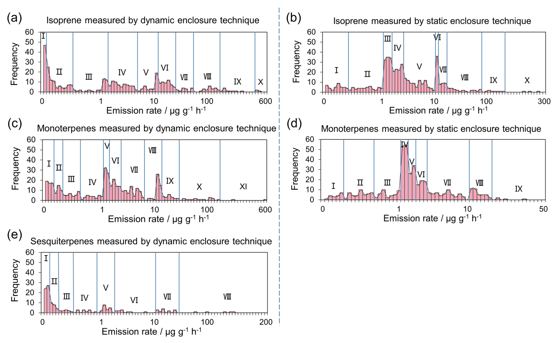
Figure 2 Frequency distribution of BVOC emission rates observed by (a, c, e) dynamic and (b, d) static enclosure techniques. The Roman numerals on each subgraph represent the emission categories identified by the frequency distribution.

For each category, the ranges, frequency, mean, and standard deviation (SD) of emission rates are listed in Table 1. The frequencies of emission rates varied among emission categories. For the measurements by the dynamic enclosure technique, isoprene emission rates were concentrated in category II, ranging 0.05–0.5 $\mathrm{\mu }\mathrm{g}{\mathrm{g}}^{-\mathrm{1}}{\mathrm{h}}^{-\mathrm{1}}$, with a frequency of 22 %; categories VII–X, with higher emission intensity, comprised only 13 % of the total measurements. This indicates that the categories with low and moderate emission intensity included the most plant species and samples. The distribution of monoterpene emission rates measured by the dynamic technique was relatively uniform, with frequencies ranging from 11 %–16 % in most categories. For sesquiterpenes, category I, with the lowest emission intensity had the most measurements, accounting for 36 % of the total, indicating the generally lower sesquiterpene emissions for most plants. Among the emission rates measured by the static technique, the highest frequencies of isoprene and monoterpene emission rates were found in categories III and IV, respectively; their lowest frequencies occurred in categories with the highest emission intensity, comprising less than 2 % of the total measurements.

Table 1 Emission categories and their emission rate ranges and statistical results for each BVOC component.

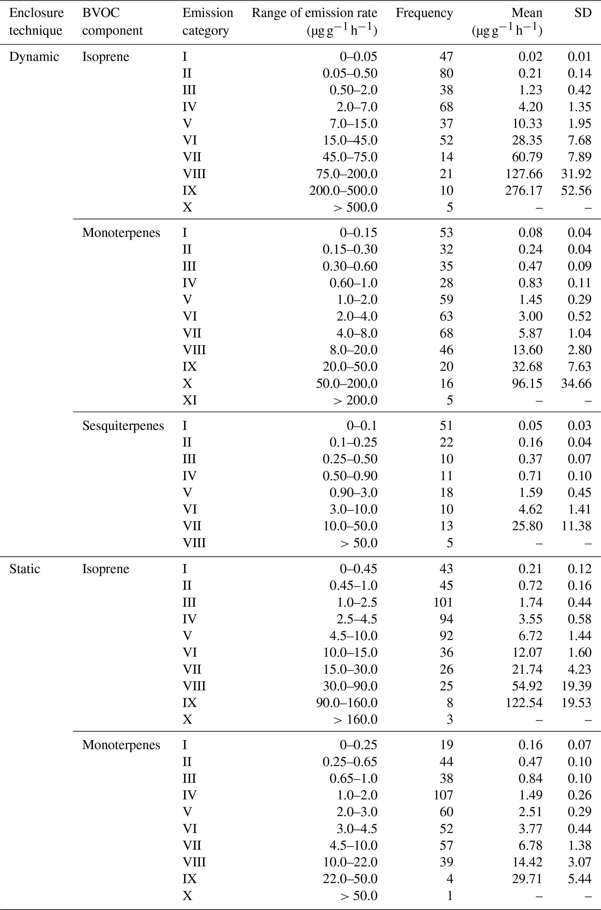
The emission rates exhibited a discrete distribution within each emission category, characterized by large SDs relative to the mean. Using the mean as the representative emission rate for each category would introduce uncertainty in emission rates for individual plant species. Therefore, to obtain a robust estimate of the central tendency that is less sensitive to potential outliers and the large observed variance, we implemented a two-step statistical protocol to determine the representative emission rates for each category. First, the 95 % confidence interval (CI) of each emission category was determined through a t test (Rivas-Ruiz et al., 2013). This allowed a 95 % probability of the actual emission rates falling within each category. Second, the values within the 95 % CI for each category were averaged as its representative emission rate. Third, the emission rate interval for each intensity category was determined by ±50 % of its representative value. Notably, for the category with the highest emission intensity, the lower limit of the interval was taken as the representative value due to its limited samples and high dispersion. Thus, the emission rate intervals and representative values for each intensity category were obtained specifically for each BVOC component and for measurements by dynamic and static techniques separately, as listed in Table S3.

For emission categories with lower emission intensity, the representative emission rates from observations using static enclosure techniques were higher than those from observations using the dynamic technique. The opposite was observed for emission categories with higher emission intensity. Specifically, for isoprene, ten emission categories were classified for observations by both techniques. The representative emission rates from the static technique were higher than those from the dynamic one in categories I–V, which had lower emission intensity, while they were lower in categories VI–X, which had higher emission intensity.

3.2.2 Determination of emission rates

Based on the established detailed categories of emission intensity with more accurate representative emission rates and intervals, the plant species-specific emission rates were determined. For a certain plant species, the assignment rule of emission rate is shown in Fig. 3. The assignment is separate for the measurements by dynamic and static techniques. Then, a localized library including BVOC emission rates for 599 plant species was constructed, including those estimated based on the measurements by both dynamic and static enclosure techniques, labeled with R values of 1 and 2, respectively. This library is available at https://doi.org/10.5281/zenodo.14557394 (Han et al., 2024).

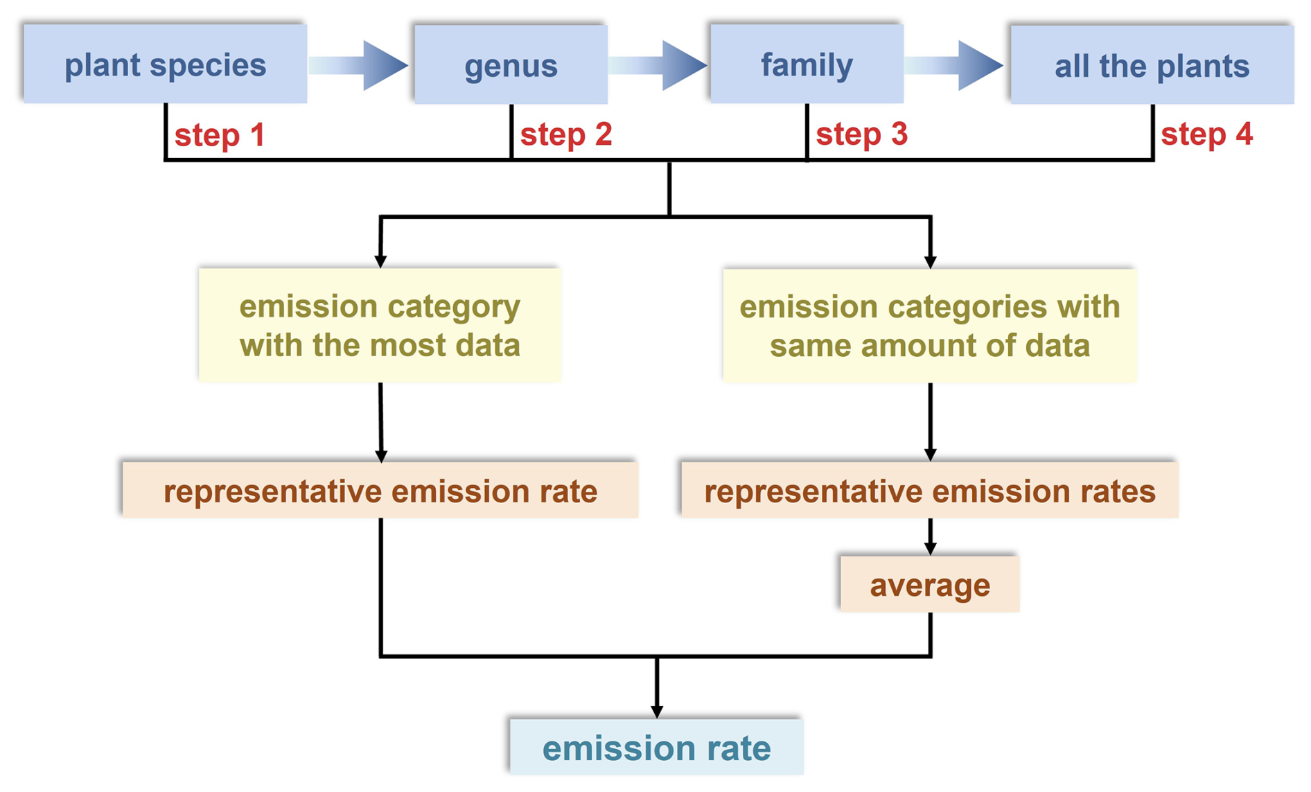
Figure 3 Determination of the emission rate for a certain plant species. Step 1–4 mean the order of priority when determining emission rates, namely using baseline data of the plant species primarily (step 1), then its belonging genus (step 2) and family (step 3), and at last all the plants in our dataset (step 4). For one of the steps, if no data fall within the interval of any emission category, then the observations of emission rates in the next step are used.

3.3 Characteristics of localized emission rate library

3.3.1 Emission intensities of plants

To characterize the emission capacitiesof different vegetation types, the number of plant species in each emission category was counted, with R value = 1 as an example (Fig. S2). First, most plant species (57 %) exhibited low-to-moderate isoprene emission intensities (Categories IV–VI). This emission profile was predominantly observed in evergreen broadleaf trees, deciduous broadleaf trees, and evergreen broadleaf shrubs, which together accounted for 69 % of the species in these categories. Crops were uniformly distributed across Categories II–VI (low-to-moderate), whereas herbs showed a wide distribution, spanning all categories except Category II. Besides, monoterpene emissions were primarily characterized by moderate intensity (Categories V–VII), encompassing 53 % of all species. Key contributors included evergreen broadleaf trees, deciduous broadleaf trees, and both evergreen and deciduous broadleaf shrubs. In contrast, only a small fraction of species (7 %) displayed high emission intensities (Categories IX–XI). Most herb species (67 %) showed moderate-to-high monoterpene emissions (Categories IV, VII, and VIII), while the majority of crop species (85 %) fell into the low-to-moderate range (Categories III–VII). As for sesquiterpene emissions, over half of the plant species (52 %) demonstrated low sesquiterpene emission intensities (Categories I–II), primarily consisting of evergreen broadleaf trees, evergreen coniferous trees, deciduous broadleaf trees, and crops. Deciduous broadleaf trees and shrubs showed a relatively uniform distribution across Categories I–VIII.

In general, most plant species emit isoprene at low to moderate intensities. Specifically, broadleaf plants predominantly exhibited a moderate emission intensity, whereas coniferous plants were mostly characterized by low-intensity emissions. Regarding monoterpenes, both broadleaf and coniferous plants primarily showed a moderate emission intensity. In contrast, herbaceous plants displayed a wide range of emission intensities for both isoprene and monoterpenes, covering low, moderate, and high levels. Meanwhile, the emission intensity of sesquiterpenes was relatively lower for most plant species, particularly trees and crops.

3.3.2 Emission differences among vegetation types

The distribution of emission rates across various vegetation types is illustrated in Fig. 4. Notably, considerable variation existed among vegetation types, characterized by a discrete distribution. For isoprene, the emission rates of trees were typically concentrated at 0.02–28.5 $\mathrm{\mu }\mathrm{g}{\mathrm{g}}^{-\mathrm{1}}{\mathrm{h}}^{-\mathrm{1}}$, those of shrubs concentrated around 4.2 $\mathrm{\mu }\mathrm{g}{\mathrm{g}}^{-\mathrm{1}}{\mathrm{h}}^{-\mathrm{1}}$, and those of crops mainly in 0.20–28.5 $\mathrm{\mu }\mathrm{g}{\mathrm{g}}^{-\mathrm{1}}{\mathrm{h}}^{-\mathrm{1}}$, while emission rates of herbs showed a discrete distribution, with an average of 26.5 $\mathrm{\mu }\mathrm{g}{\mathrm{g}}^{-\mathrm{1}}{\mathrm{h}}^{-\mathrm{1}}$. Overall, herbs showed the highest isoprene emission, followed by trees and shrubs, based on their means and medians. For monoterpenes, emission rates of trees and shrubs were primarily concentrated at 1.5–5.8 $\mathrm{\mu }\mathrm{g}{\mathrm{g}}^{-\mathrm{1}}{\mathrm{h}}^{-\mathrm{1}}$, those of crops were mainly 0.46–5.8 $\mathrm{\mu }\mathrm{g}{\mathrm{g}}^{-\mathrm{1}}{\mathrm{h}}^{-\mathrm{1}}$, while those of herbs were evenly distributed, with an average of 17.7 $\mathrm{\mu }\mathrm{g}{\mathrm{g}}^{-\mathrm{1}}{\mathrm{h}}^{-\mathrm{1}}$. Generally, herbs had the highest monoterpene emission, followed by shrubs, while the emissions of trees and crops were comparatively lower. As for sesquiterpenes, the emission rates for trees were mainly concentrated at 0.05–0.17 $\mathrm{\mu }\mathrm{g}{\mathrm{g}}^{-\mathrm{1}}{\mathrm{h}}^{-\mathrm{1}}$ and secondarily in 0.36–4.3 $\mathrm{\mu }\mathrm{g}{\mathrm{g}}^{-\mathrm{1}}{\mathrm{h}}^{-\mathrm{1}}$; those of shrubs were mainly distributed around 0.17 and 1.5 $\mathrm{\mu }\mathrm{g}{\mathrm{g}}^{-\mathrm{1}}{\mathrm{h}}^{-\mathrm{1}}$, and those of crops and herbs were mainly 0.05–0.17 $\mathrm{\mu }\mathrm{g}{\mathrm{g}}^{-\mathrm{1}}{\mathrm{h}}^{-\mathrm{1}}$. Comparatively, trees and shrubs showed the highest sesquiterpene emission, followed by herbs, while crops had the lowest emission. As to the subtypes, broadleaf plants had relatively higher isoprene emission levels, while coniferous plants had higher monoterpene emission levels. This may be attributed to the broad and thick leaves of broadleaf plants, which possess stronger photosynthetic efficiency to produce isoprene (Benjamin et al., 1996; Li et al., 2021). Meanwhile, the thicker cuticle of coniferous plants can create favorable conditions for the storage of monoterpenes (Aydin et al., 2014), which are primarily regulated by temperature and less influenced by light (Bourtsoukidis et al., 2024). Moreover, the vegetation types with high sesquiterpene emissions were similar to those with high monoterpene emissions, which can be explained by the significant correlation between the emissions of monoterpenes and sesquiterpenes from plants (P<0.05) reported by Ormeño et al. (2010).

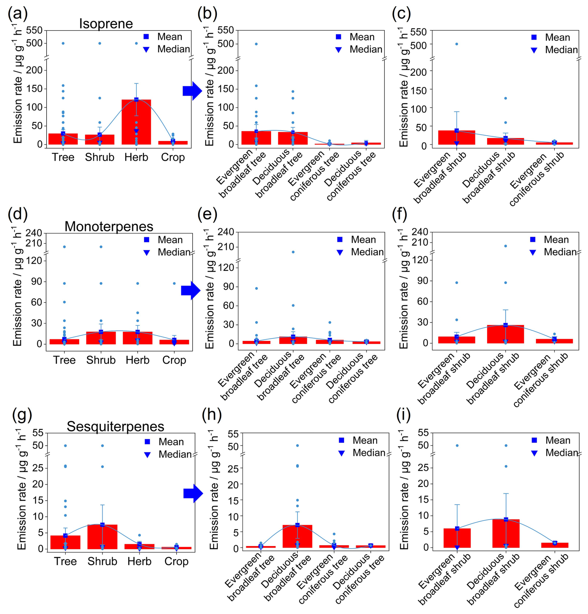
Figure 4 Statistics of BVOC emission rates in various vegetation types. (a–i) Distribution of emission rates for isoprene (a), monoterpenes (d), and sesquiterpenes (g) across vegetation types (trees, shrubs, herbs, and crops). Differences in BVOC emission rates between various subtypes of trees (b, e, h) and shrubs (c, f, i). Bar charts display median and mean of the distribution; bar ends represent the 25th and 75th percentiles, and outliers are also displayed.

3.3.3 Interspecific differences in the same family/genus

Plants within the same family or genus usually share similar morphological and biological traits (Lun et al., 2020; Wu, 2021). However, BVOC emissions are influenced by genes and interactions with the environment (Peñuelas and Staudt, 2010), leading to variations in the components and quantities of BVOC emissions. From our developed emission rate library, higher BVOC emissions were discovered in the families Poaceae and Fabaceae, which respectively had higher isoprene and monoterpene emissions. Exceptionally, the crop isoprene emission rates in Fabaceae were overall higher than those in Poaceae (Fig. 5). Specifically, the emission rates of Arachis hypogaea and Glycine max (28.5 $\mathrm{\mu }\mathrm{g}{\mathrm{g}}^{-\mathrm{1}}{\mathrm{h}}^{-\mathrm{1}}$) – belonging to Fabaceae – were higher than those of Zea mays and Sorghum bicolor (16.4 $\mathrm{\mu }\mathrm{g}{\mathrm{g}}^{-\mathrm{1}}{\mathrm{h}}^{-\mathrm{1}}$), belonging to Poaceae. Differences may exist among genera within the same family. Plants of Poaceae are widely distributed in China and worldwide (Sun et al., 2024; Wanasinghe et al., 2024), including the dominant crops like Triticum aestivum, Oryza sativa, and Z. mays, as well as herbs and bamboo. The plant species, genera, and BVOC emission rates within Poaceae are listed in Table S4. The evergreen broadleaf trees and bamboo species – such as Fargesia spathacea and Bambusa textilis – are widely distributed and commonly used for afforestation (Yan et al., 2024). They possessed the highest isoprene emission rate of 500.0 $\mathrm{\mu }\mathrm{g}{\mathrm{g}}^{-\mathrm{1}}{\mathrm{h}}^{-\mathrm{1}}$. In the selection of plant species for future afforestation, lower-emission bamboo species like Bambusa ventricosa and Bambusa vulgaris var. striata should be preferred. Herbs usually showed higher isoprene and monoterpene emissions, but Phragmites australis had higher sesquiterpene emissions. Crops showed higher sesquiterpene emissions than other vegetation types. Also, it is worth mentioning that considerable differences in emission rates were exhibited even among plants belonging to the same genus. Thus, it may introduce uncertainties to our developed emission rate library when assigning based on the observations of all the plants within the same genus or family. Meanwhile, the limited samples in the same family likely resulted in an incomplete conclusion. Therefore, expanding emission observations to cover a wider range of plant species is imperative for the development of a more precise emission rate library. Also, the accuracy of the emission rates in the developed library derived by this assignment could be verified through field observations in a future study.

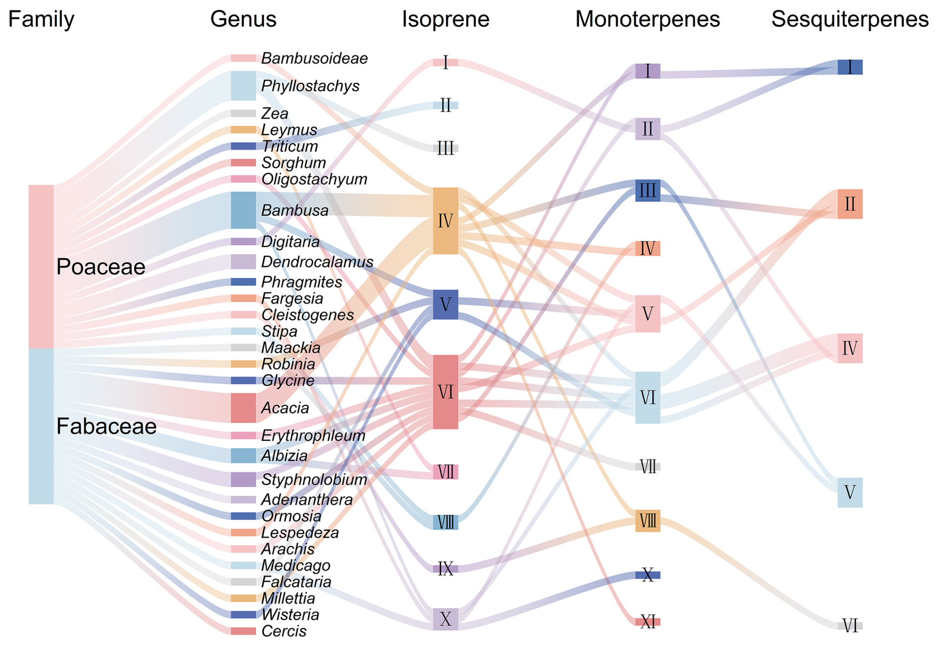
Figure 5 Emission categories of the plant species in different genera of the families Poaceae and Fabaceae. Box length represents the number of species, and colors at the start and end of each connecting line correspond to the two connected ends.

3.3.4 Variability in emission rates derived from dynamic and static enclosure measurements

In the localized emission rate library, the subsets of emission rates with R values of 1 and 2 were separately established. For isoprene emission rates, 51 % of plant species exhibited higher values with R value = 2 than with R value = 1. Among these plants, 66 % had an emission rate of 0.02–4.2 $\mathrm{\mu }\mathrm{g}{\mathrm{g}}^{-\mathrm{1}}{\mathrm{h}}^{-\mathrm{1}}$ (in lower emission intensity) (Fig. 6). In contrast, for plants with emission rates of R value = 1 higher than those of R value = 2, 78.1 % had emission rates of 28.5–500.0 $\mathrm{\mu }\mathrm{g}{\mathrm{g}}^{-\mathrm{1}}{\mathrm{h}}^{-\mathrm{1}}$ (in moderate and high emission intensity). For monoterpene emission rates, 49 % of plant species displayed higher values with R value = 2 than with R value = 1, with all emission rates below 13.4 $\mathrm{\mu }\mathrm{g}{\mathrm{g}}^{-\mathrm{1}}{\mathrm{h}}^{-\mathrm{1}}$ (in lower emission intensity). In contrast, for plants with emission rates of R value = 1 higher than those of R value = 2, 48 % had emission rates of 13.4–200.0 $\mathrm{\mu }\mathrm{g}{\mathrm{g}}^{-\mathrm{1}}{\mathrm{h}}^{-\mathrm{1}}$ (in moderate and high emission intensity). To conclude, the emission for plants with high intensity may be underestimated when measured by the static enclosure technique, while those for plants with low intensity may be overestimated. The discrepancy between emission rates derived from dynamic and static enclosure measurements is likely attributed to two factors. First, static enclosure technique, which may induce a large buildup of BVOCs and release of stressed compounds due to altered chamber conditions; its detection limit causes more compounds to be detected (Li et al., 2019), leading to higher emission rates than dynamic measurement for plants with low emission intensity. Second, plants with high emission intensity often have strong transpiration, leading to moisture condensation on the walls within the static enclosure, followed by stomatal closure and reduced emissions (Kfoury et al., 2017). In addition, high BVOCs concentrations may undergo reactions and degradation in the chamber (Antonsen et al., 2020), together contributing to underestimates by the static technique for plants with high emission intensity.

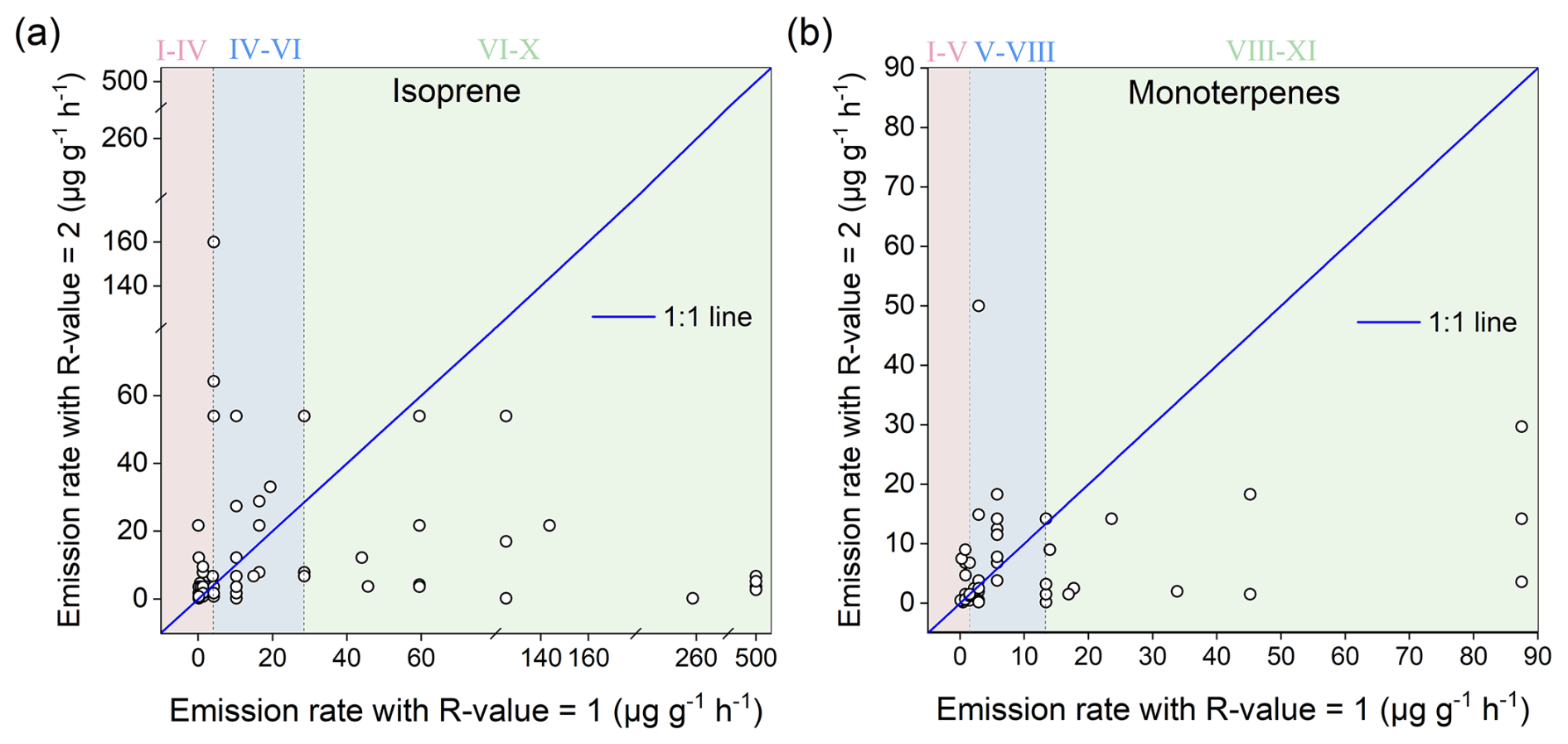
Figure 6 Comparison of emission rates derived from dynamic (R value = 1) and static (R value = 2) enclosure measurements for isoprene (a) and monoterpenes (b). (The solid line represents the 1:1 relationship, and the Roman numerals on each subgraph represent the emission category.)

3.3.5 Comparison with global emission rate library of MEGANv3.2

Comparison between our library and MEGANv3.2 global library was performed. For consistency, the comparison was conducted at the genus level, as the global library often assigns uniform values across species within a genus. Our results revealed consistent identification of high-emitting genera but quantitative differences (Fig. S4). For isoprene, while genera like Populus and Quercus are high-emitters in both libraries, our localized emission rates for Populus (78.51 $\mathrm{nmol}{\mathrm{m}}^{-\mathrm{2}}{\mathrm{s}}^{-\mathrm{1}}$) and Salix (11.64 $\mathrm{nmol}{\mathrm{m}}^{-\mathrm{2}}{\mathrm{s}}^{-\mathrm{1}}$) differ significantly from the global value (37 and 37 $\mathrm{nmol}{\mathrm{m}}^{-\mathrm{2}}{\mathrm{s}}^{-\mathrm{1}}$, respectively). The discrepancies are even more pronounced for monoterpenes. Genera Lespedeza and Spiraea have the highest emissions in both libraries, but the localized values (40.87 and 21.0 $\mathrm{nmol}{\mathrm{m}}^{-\mathrm{2}}{\mathrm{s}}^{-\mathrm{1}}$) are nearly an order of magnitude higher than the global values (5.30 and 2.73 $\mathrm{nmol}{\mathrm{m}}^{-\mathrm{2}}{\mathrm{s}}^{-\mathrm{1}}$). In contrast, sesquiterpene emissions show closer agreement in both libraries.

4 Application of localized emission rate library

4.1 BVOC emission simulation

MEGANv3.2 was applied to estimate BVOC emissions, including 199 compounds (isoprene, 40 monoterpenes, 45 sesquiterpenes, and 113 other VOCs). The simulation was driven by key inputs, including vegetation data, species-specific emission rates, and externally sourced meteorological fields such as Weather Research and Forecasting (WRF) output. Specifically, the vegetation data include the distribution of four growth forms, their species speciation, ecological types, canopy types, and leaf area index (LAI). In the study, the database of high-resolution vegetation distribution (HRVD) with a horizontal resolution of 1 km×1 km established by Cao et al. (2024b, https://doi.org/10.5281/zenodo.10830151), was used to produce the distributions of growth forms and canopy types. It integrates multiple sources of land cover data – including the China multi-period land use/cover change remote sensing monitoring data set (CNLUCC) (Xu et al., 2020), MODIS MCD12Q1 land cover product (Friedl and Sulla-Menashe, 2019), as well as the Vegetation Atlas of China (1:1 000 000) – which shows a significant correlation with the field investigation. The vegetation speciation was derived from the Vegetation Atlas of China (1:1 000 000). LAI was from the MODIS version 6.1 LAI product reprocessed by Lin et al. (2023) (http://globalchange.bnu.edu.cn/research/laiv061, last access: 16 May 2025) and further updated based on the HRVD. Hourly meteorological fields driving MEGANv3.2 were simulated by WRF v3.8.1. The simulation covered the whole of China at a horizontal resolution of 36 km×36 km for the year 2020.

In MEGAN version 3.2 used in this study, both PFT distribution and detailed vegetation species composition in grids are entered. Based on the vegetation composition, the gridded PFT-averaged emission factors can be calculated from the species-specific emission factors using the emission factor processing module of MEGANv3.2 and are then included in the emission calculator. Notably, plant species in our library did not cover all the plants in the vegetation speciation file; for species not included in our library, we assigned their emission factors using the global values. To match the input for MEGANv3.2, where monoterpenes and sesquiterpenes were categorized into five and two categories, respectively, the emission rates of monoterpenes and sesquiterpenes were assigned to separate categories based on the relationships of the global ones in MEGANv3. In total, emission rates of 283 plant species were updated, including 257, 280, and 101 species for isoprene, monoterpenes, and sesquiterpenes, respectively. Specifically, 202 plant species the emission rates with R value = 1, while an additional 81 species had those with R value = 2. The application of emission rates with R value = 1 was assessed by calculating the plant species coverage percentage of the total vegetation. Emission rates with R value = 1 cover a high percentage of the dominant vegetation, specifically 93 % of the total tree area and 94 % of the total crop area. In contrast, their coverage is substantially lower for shrubs and herbs, with 34 % and 21 % of their respective areas. This is a common challenge in regional BVOC modeling, as comprehensive field measurements for all shrub and herb species are often limited.

To systematically evaluate the performance of the localized emission library developed in this study, four simulation experiments (Simulation 1–4) were conducted under identical model configurations, with the only variation being the source of emission rates. Simulation 1 incorporated all available species-specific emission rates in our localized library, prioritizing those with high accuracy (R value = 1) and supplementing with lower-accuracy records (R value = 2) where necessary, thereby maximizing localization. Simulation 2 used only R value = 1 emission rates to establish a baseline under the most reliable data scenario. Simulation 3 also employed the full localized library but favored R value = 2 data and supplemented it with R value = 1. This design enabled a controlled assessment of data quality influence through comparison with Simulation 1. In Simulations 1–4, for plants without assigning localized emission rates, global data were used. Finally, Simulation 4 relied on the default global emission rate library embedded in MEGANv3.2, serving as a reference to quantify the net effect of emission rate localization when compared with Simulation 1. A summary of the simulation design is provided in Table 2 for clarity.

Table 2 Simulation experiments for evaluation of the localized emission rate library.

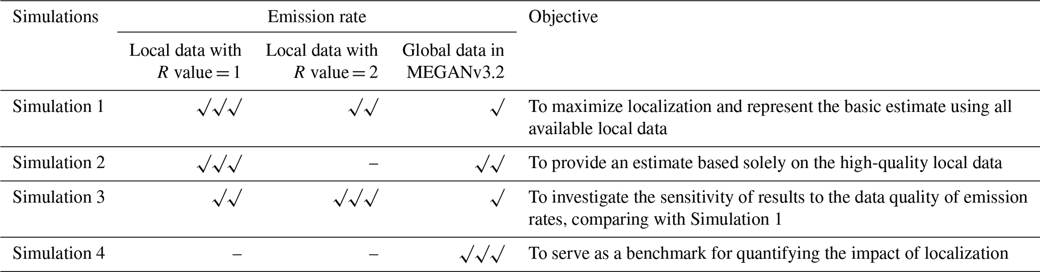
Note: The number of √ symbols shows the priority from high to low. Taking Simulation 1 as an example, the plant species-specific emission rates are assigned from the localized library with R value = 1 primarily (labeled $\surd \surd \surd$), then those with R value = 2 as a supplement (labeled $\surd \surd$), and global data are used for plants without localized emission rates (labeled √).

4.2 BVOC emissions in China

Based on the results in Simulation 1 where our developed emission rate library was fully applied – including the emission rates with R values of both 1 and 2 (as in Table 2) – the annual total BVOC emission in China for the year 2020 was 27.70 Tg (detailed composition shown in Fig. S5). In the four BVOC categories, other VOCs contributed the most, accounting for 47 % of the total emissions. The large contribution was attributable to their large number of compound species, comprising more than half of the total simulated compounds in MEGANv3.2. Isoprene and monoterpenes exhibited comparable contributions, accounting for 23 % and 25 % of the total, respectively. Specifically, isoprene, butane, and isobutene emerged as the most substantial contributors to BVOC emissions, jointly accounting for 44 %. Notably, in our study, the emission estimates for butane and isobutene used global emission factors without localization. They were even higher than the isoprene and monoterpene emission factors from our localized library for some tree species. This might have introduced uncertainties, and local observations for their emission rates are required in the future.

BVOC emissions in China exhibited large spatial variations, higher in the southeast and lower in the northwest (Fig. 7). Specifically, high emissions in the Southeast Hill, Yunnan–Guizhou Plateau, and Taiwan Province, located in southeastern China, were primarily attributed to the extensive coverage of evergreen broadleaf trees (Cai et al., 2024). Among them, the widely distributed plants Quercus fabri, Bambusa textilis, and Lithocarpus amygdalifolius had higher isoprene emission rates of 85.5, 500.0, and 125.4 $\mathrm{\mu }\mathrm{g}{\mathrm{g}}^{-\mathrm{1}}{\mathrm{h}}^{-\mathrm{1}}$, respectively. Suitable environments characterized by high temperatures were also major contributors to the high emissions in these regions (Duan et al., 2023). Furthermore, the Greater and Lesser Khingan Mountains and Changbai Mountains were rich in forest resources, including both coniferous and broadleaf trees, accounting for over 77 % of the total vegetation distribution in those regions, resulting in relatively higher BVOC emissions. The North China Plain and Sichuan Basin, with their widespread crop cultivation, accounting for 74 % and 54 % of the total vegetation coverage, also exhibited high emissions. The lower emissions in the northwest were likely due to the predominance of herb species with lower emission rates, such as Festuca ovina, Krascheninnikovia compacta, and Elymus nutans.

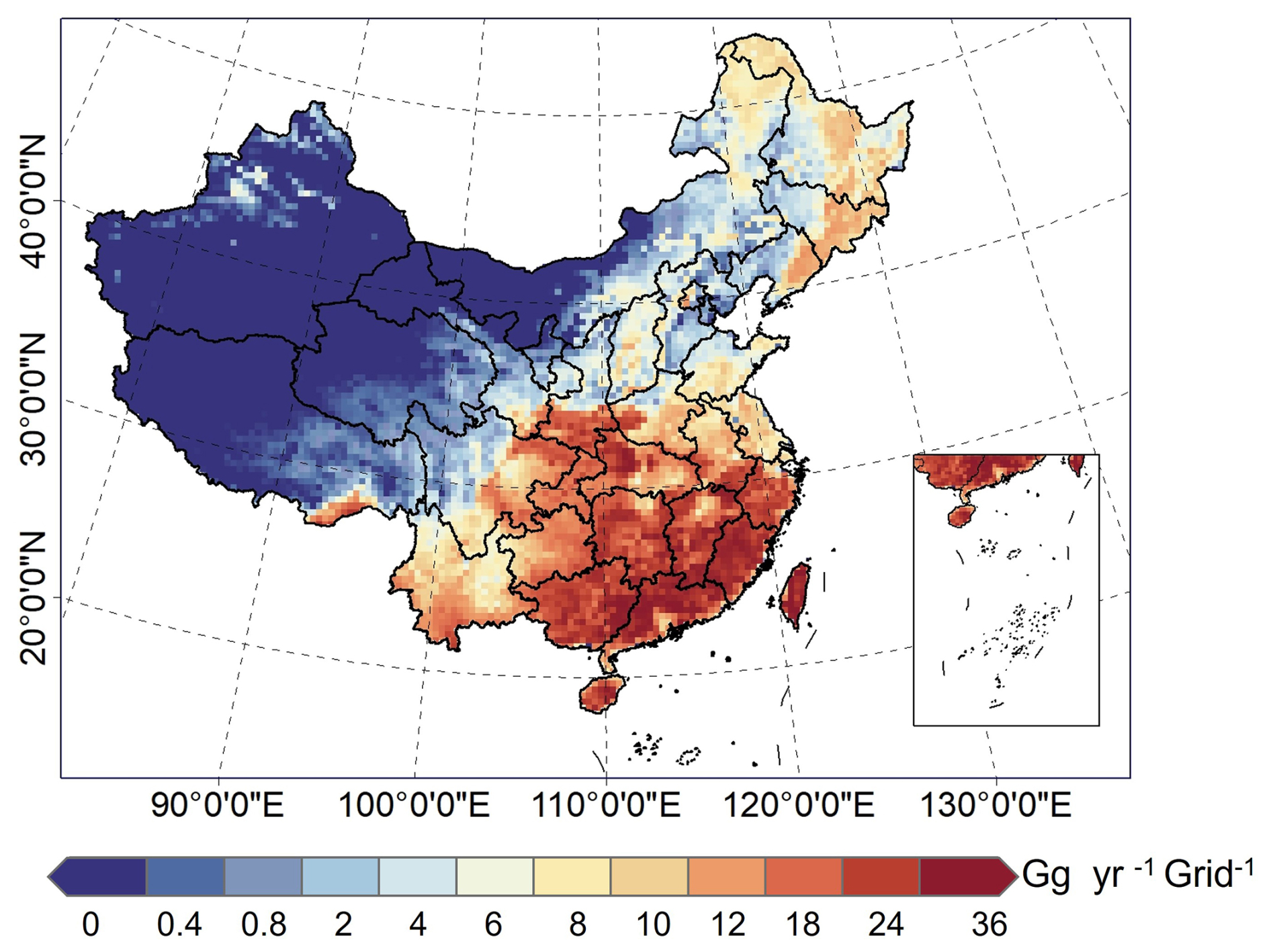
Figure 7 Spatial distribution of BVOC emissions estimated based on the localized emission rate library in China in 2020.

Compared with the results in Simulation 4, BVOC emissions were 18 % higher after updating the emission rates using our developed library than the emissions (23.44 Tg) estimated using the global emission rates without localization. By BVOC categories, the emissions of isoprene, monoterpenes, and sesquiterpenes increased by 55 %, 29 %, and 48 %, respectively. The contributions of isoprene, monoterpenes, sesquiterpenes, and other VOCs to total BVOC emissions changed from 18 %, 23 %, 4 %, and 55 % to 23 %, 25 %, 5 %, and 47 %, respectively. A discrepancy was also found in the spatial distribution (Fig. 8c). In southeastern China, especially the Sichuan Basin, Simulation 1 showed higher emissions than Simulation 4. This was likely due to the widespread distribution of crops, which had higher emission rates in our library compared with the global one. Conversely, in western and northeastern China, particularly in the Greater and Lesser Khingan Mountains and Changbai Mountains, emissions in Simulation 1 were lower than in Simulation 4. This was mainly due to the extensive distribution of the genera Pinus and Betula. Their isoprene emission rates with R value = 1 were used in Simulation 1, which were 80 % and 86 % lower than the global ones, respectively. Also, the plants of the two genera were widespread, accounting for 70 % of the total vegetation coverage area in the Greater and Lesser Khingan Mountains and Changbai Mountains. To evaluate the spatial patterns of simulated BVOC emissions based on various emission rates, the correlation between emissions and observed formaldehyde (HCHO) vertical column density (VCD) was analyzed. HCHO in the atmosphere can serve as a reliable proxy for tracing the biogenic source of isoprene, especially in summer (Liu et al., 2024). Here, the Sentinel-5p TROPOspheric Monitoring Instrument (TROPOMI) Spaceborne HCHO products, which can be accessed through the Google Earth Engine platform (https://code.earthengine.google.com/, last access: 10 June 2025), were used. It is important to note that in our study region, which is subject to anthropogenic influences, a substantial fraction of the atmospheric HCHO is expected to originate from anthropogenic VOCs (Ren et al., 2022). This likely caused uncertainty in our analysis, in summer. Meanwhile, satellite HCHO products also exhibit uncertainties (Chong et al., 2024). As shown in Fig. S7, the isoprene emissions in July in Simulation 1 correlated more strongly with HCHO concentration spatially (correlation coefficient = 0.73, P<0.05) than in Simulation 4 (correlation coefficient = 0.67, P<0.05). This suggests that the application of our localized emission rate library could simulate the spatial variations of BVOC emissions better. Using the global emission rate library, there might be an underestimate in the south and an overestimate in the northeast and west, which could be abated by updating the localized emission rates.

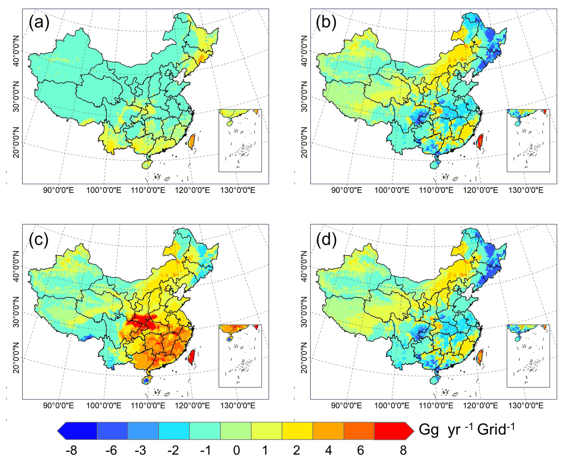
Figure 8 Spatial distribution of differences among BVOC emissions simulated using different emission rates: (a–d) Simulation 1 minus Simulation 2 (a), Simulation 1 minus Simulation 3 (b), Simulation 1 minus Simulation 4 (c), Simulation 2 minus Simulation 3 (d).

4.3 Impact of emission rates with different reliability on BVOC emission estimates

To apply more accurate emission rates, Simulation 2 was conducted employing only the emission rates with R value = 1 from the localized library. For the plant species having emission rates with R value = 2 in Simulation 1, the global emission rates were assigned in Simulation 2. Compared with the estimation from Simulation 1, there was a similar total emission (27.46 Tg). By BVOC categories, isoprene emissions increased by 4 %, while monoterpene emissions decreased by 2 %; the emissions of sesquiterpenes and other VOCs remained unchanged. The BVOC composition changed little. Spatially, in most regions of China, the emissions of Simulation 1 were slightly lower than those from Simulation 2 by −1 to 0 $\mathrm{Gg}{\mathrm{yr}}^{-\mathrm{1}}{\mathrm{grid}}^{-\mathrm{1}}$ (Fig. 8a). The main reason for this discrepancy was that plant emission rates were updated using R value = 2 in Simulation 1, which was lower than the global ones in Simulation 2. Among these plants, herbs accounted for 84 %, while trees and shrubs only accounted for 3 % and 14 %, respectively. The average isoprene and monoterpene emission rates of these herb species derived from our library were 7 % and 67 % lower than those from the global library, respectively. In contrast, the emissions of Simulation 2 exceeded those of Simulation 1 in certain areas by $\mathrm{0}-\mathrm{6}\mathrm{Gg}{\mathrm{yr}}^{-\mathrm{1}}{\mathrm{grid}}^{-\mathrm{1}}$, which were concentrated in South China, the Lesser Khingan Mountains, and the Changbai Mountains. This was primarily due to the herb distribution belonging to the Carex genus, whose isoprene emission rates with R value = 2 were 24 % higher than the global values. These plants comprised 31 % of the total herb coverage. The above resulted in only small changes in the national total BVOC emissions when excluding emission rates with lower reliability.

Furthermore, to investigate the impact of using emission rates with R value = 1 versus R value = 2 on the estimated emissions, Simulation 3 was conducted by using those with R value = 2 preferentially and then those with R value = 1 supplementally. The results in Simulations 1 and 3 were compared. Simulation 3 produced an increase in BVOC emissions by 7 %. By BVOC categories, isoprene and monoterpene emissions rose by 17 % and 11 %, respectively, while those of sesquiterpenes and other VOCs remained similar. Their contributions to the total BVOC emissions changed little. Spatially, in most regions, the emissions in Simulation 3 were higher than those in Simulation 1 (Fig. 8b), particularly in the Sichuan Basin. O. sativa, a single crop species, accounted for 93 % of the total crop coverage. Its isoprene and monoterpene emission rates for R value = 2 were 1.2 and 14.2 $\mathrm{\mu }\mathrm{g}{\mathrm{g}}^{-\mathrm{1}}{\mathrm{h}}^{-\mathrm{1}}$, respectively, much higher than those with R value = 1 (0.18 and 5.8 $\mathrm{\mu }\mathrm{g}{\mathrm{g}}^{-\mathrm{1}}{\mathrm{h}}^{-\mathrm{1}}$). In the Lesser Khingan Mountains and Changbai Mountains, the isoprene emission rate for the widely distributed genus Larix with R value = 2 was 166 % higher than that with R value = 1; for the species Pinus koraiensis, the monoterpene emission rate with R value = 2 was 390 % higher. Conversely, in areas where herbs were widely distributed, especially in the northwest of China, the emissions in Simulation 3 were lower than those in Simulation 1. This was likely because, for most herb species, emission rates at R value = 2 were lower than those at R value = 1. For instance, the applied isoprene emission rates for the genera Stipa, Cleistogenes, and Leymus in Simulation 1 were 125.8, 258.9, and 59.5 $\mathrm{\mu }\mathrm{g}{\mathrm{g}}^{-\mathrm{1}}{\mathrm{h}}^{-\mathrm{1}}$, respectively, while they were 1.2, 1.2, and 4.2 $\mathrm{\mu }\mathrm{g}{\mathrm{g}}^{-\mathrm{1}}{\mathrm{h}}^{-\mathrm{1}}$, respectively, in Simulation 3. For emissions estimated in Simulation 3, the correlation between emissions and observed HCHO VCD was analyzed, with a correlation coefficient of 0.63 (P<0.05). Meanwhile, the correlation coefficient (0.72) for the emissions estimated in Simulation 2 was also higher than that in Simulation 3. Their correlation coefficient was 0.63 (P<0.05), lower than that in Simulation 1. Meanwhile, the correlation coefficient (0.72) for the emissions estimated in Simulation 2 was also higher than that in Simulation 3. Therefore, it can be concluded that greater application of emission rates from dynamic measurements leads to better implications for emission estimates. Together with maximizing localization, namely using emission rates from static measurements as a supplement, better results will be obtained. Notably, similar national total BVOC emissions and spatial accuracy were observed between Simulations 1 and 2 because most of the species (84 %) with emission rates of R value = 2 were herbs, whose coverage was limited. Overall, using emission rates with R value = 2 could overestimate total BVOC emissions in China. Therefore, additional high-reliability emission observations using dynamic techniques are strongly encouraged to further improve the accuracy of the localized emission rate library and emission inventory.

5 Conclusion

By integrating our field measurements with reported local measurements, a statistical approach for classifying emission categories and determining plant species–specific emission rates for BVOC emission inventory compilation was developed. It produced more detailed categories of emission intensity, accurate emission rate intervals, and representative values compared to previous studies, namely ten, ten or eleven, and eight categories respectively for isoprene, monoterpene, and sesquiterpene emission rates. The detailed categories for emission intensity can further improve the determined representative emission rates. Based on this, a localized plant species–specific BVOC emission rate library for China was developed, including isoprene, monoterpene, and sesquiterpene emission rates for 599 plant species. In this library, observations from both dynamic and static techniques were included and separated with different reliability. Variability was found in the emission rates derived from dynamic and static enclosure measurements. Specifically, measurements by static enclosure technique may underestimate the emissions of plants with higher emission intensity and overestimate the emissions of plants with lower emission intensity. Analyzing the emission rates derived from the dynamic technique measurements in our library, and comparing the means and medians among vegetation types, herbs showed the highest isoprene emission level, followed by trees and shrubs; herbs also had the highest monoterpene emission level, followed by shrubs, while trees and crops were comparatively lower; trees and shrubs showed the highest sesquiterpene emission levels, followed by herbs and crops. Interspecific differences were exhibited within the same type, family, or genus.

Furthermore, our localized emission rate library was applied in China's BVOC emission inventory compilation, with performance evaluation. By updating the localized emission rates, the simulated BVOC emission in China in 2020 was 27.70 Tg, 18 % higher than that using the global emission rate library. Isoprene, monoterpenes, sesquiterpenes, and other VOCs contributed 23 %, 25 %, 5 %, and 47 % to the total emissions, respectively. It had better performance in emission estimation, with the higher correlation coefficient of 0.73 (P<0.05) between isoprene emission and HCHO VCD observations spatially. The underestimates in the south and overestimates in the northeast and west when using global emission rates could be reduced by updating the localized ones. Using emission rates with different reliability could result in different emission estimates and model performance. The use of emission rates measured by static enclosure technique could decrease the accuracy of estimation and result in an overestimation of BVOC emissions. Therefore, in BVOC emission inventory compilation, it is suggested to use emission rates measured by the dynamic enclosure technique more to achieve more accurate results.

Although our developed localized emission rate dataset is beneficial for improving the accuracy of the emission inventory, uncertainties still exist in the dataset and its application. First, the dataset includes only a limited number of plant species, making it difficult to cover all the plants in China. Researchers must use global emission rates for plants without localized observations. Second, uncertainties may be introduced when assigning emission rates based on observations of plants within the same genus or family. For the emission rates with R value = 1, 16 % were allocated by genus and 13 % by family; for those with R value = 2, 3 % were allocated by genus and 5 % by family. Third, for monoterpene and sesquiterpene emission rates separately, some of the raw observed results are the sum of their studied dominant compounds rather than the whole category of monoterpenes and sesquiterpenes. Therefore, in the application of our dataset, there may be an underestimation of their emissions. Meanwhile, the MEGAN model requires more detailed categories for them; it is better to conduct compound-specific observations and obtain their emission rates. Fourth, the determined emission categories can be more detailed, and the emission rate intervals and representative values can be more accurate if more local observation samples are available. The above uncertainties would be reduced by including more reliable local emission measurements, specifically by plant species and compounds, in the future. Notably, despite the current uncertainties, our study starts the effort to establish a reliable localized dataset of BVOC emission rates used in inventory compilation. Undeniably, it helps improve the regional representativeness of model inputs for China and better captures the spatial variations of BVOC emissions. Meanwhile, our developed statistical approach can be extended to the establishment of localized BVOC emission rate datasets for other regions.