The boundary of nighttime ozone chemical equilibrium as an indicator of local chemistry disturbances in the polar mesopause region

The nighttime ozone chemical equilibrium (NOCE) is a key assumption widely employed in various applications within the mesopause region, such as retrieving difficult-to-measure characteristics from observational data. Previously, the NOCE boundary criterion was used to analyze its long-term evolution based on SABER/TIMED data, primarily at low and mid-latitudes. This study extends this focus to polar latitudes. We demonstrate that the NOCE criterion clearly delineates the main features of the transition zone that vertically separates regions of strong and weak diurnal photochemical oscillations of O and H. During the polar night, this transition zone degenerates into a sharp step in the vertical profiles of these species, and the criterion accurately identifies the altitude of this step. Furthermore, we analyze the evolution of the NOCE boundary using SABER/TIMED observations in conjunction with MERRA-2 reanalysis data for the winter–spring periods from 2002 to 2025. We show that the most pronounced variability of the NOCE boundary occurs at northern polar latitudes during and after strong Sudden Stratospheric Warmings accompanied by stratopause elevation events. Prior to or during the onset of such warmings, the daily mean altitude of the boundary can rise to ∼86 km. Following these events, it rapidly descends to 72–74 km, where it can remain for an extended period. Model studies of the 2009 winter show that the NOCE boundary closely tracks the variability of the median vertical distributions of O, as well as the volume emission rates of OH(v=1–9), O(¹S), and O₂(b${}^{\mathrm{1}}{\mathrm{\Sigma }}_g^{+}$).

1 Introduction

Ozone is a unique atmospheric trace gas that plays different roles depending on altitude. In particular, stratospheric ozone protects life on our planet by absorbing ultraviolet solar radiation in the wavelength range of 200–315 nm. Moreover, by absorbing radiation in the Herzberg continuum, ozone at these altitudes is the only atmospheric minor gas whose vertical distribution determines the photodissociation rate of the major gas, molecular oxygen. In turn, tropospheric ozone acts as the fourth (in terms of importance) greenhouse gas after H₂O, CO₂ and CH₄. Furthermore, in the boundary layer, ozone is one of the five major pollutants (according to the World Health Organization) that negatively affect the biosphere and human health due to its high toxicity.

In the mesosphere–lower thermosphere (MLT), ozone is involved in reactions between the O_x and HO_x families (O+O₃ and $\mathrm{H}+\mathrm{OH}+{\mathrm{HO}}_{\mathrm{2}}$), which produce many layered phenomena. Below ∼80–87 km, there are strong diurnal photochemical oscillations, where the difference between daytime and nighttime values of these components can reach several orders of magnitude due to the diurnal modulation of the photodissociation rates of O₂, H₂O, and O₃. Above ∼80–87 km, photochemical oscillations are relatively weak compared to the more pronounced impact of vertical and horizontal transport. As a result, there is a narrow (1–3 km thick) transition region where the regime of photochemical oscillations changes rapidly with height. Above this transition region, O and H concentrations accumulate and reach absolute maxima, forming the corresponding layers, including a layer of stored chemical energy. This leads to the appearance of a secondary ozone maximum and airglow layers of excited OH, O₂ and O observed in the visible and infrared ranges. In particular, the reaction of ozone with atomic hydrogen is the main source of OH airglow, whose intensity spectrum can be used, for example, to derive information about the mesopause temperature. Thus, mesopause photochemistry enables several remote sensing techniques that are widely used for ground-based and satellite monitoring of climate change and wave activity at these altitudes. The chemical heating from exothermic reactions between O_x-HO_x species is one of the major sources of the mesopause energy balance. In particular, this heating can exceed that from turbulent energy dissipation (e.g., Grygalashvyly et al., 2024). Moreover, mesopause photochemistry influences the radiative cooling of this region in the CO₂ 15 µm band, is involved in plasma-chemical reactions, and contributes to the formation of ionospheric layers. Note that variations in the O_x-HO_x transition zone height reflect corresponding changes in the O and H layers, and through them, in airglows and other mesopause features. Thus, this characteristic can be considered a sensitive indicator of mesopause processes.

Note also, the mentioned transition of O_x-HO_x behavior with height may occur via the nonlinear response to the diurnal modulation of photodissociation rates, resulting in the appearance of subharmonic (with periods of 2, 3, 4, and more days) or chaotic oscillations of O, O₃, H, OH, and HO₂ (e.g., Sonnemann and Fichtelmann, 1997; Feigin et al., 1998). This unique phenomenon was investigated theoretically by taking into account different transport processes (Sonnemann and Feigin, 1999; Sonnemann et al., 1999; Kulikov and Feigin, 2005; Kulikov, 2007; Kulikov et al., 2020), including within the framework of the 3D chemical-transport models (Sonnemann and Grygalashvyly, 2005; Kulikov et al., 2021). The vertical eddy diffusion was revealed as the most important process (Sonnemann and Feigin, 1999; Sonnemann et al., 1999), so that 2 d oscillations can only survive at real diffusion coefficients. At the same time, the eddy diffusion in the zonal direction leads to the appearance of the so-called reaction-diffusion waves in the form of propagating phase fronts of 2 d oscillations (Kulikov and Feigin, 2005; Kulikov et al., 2012; Kulikov et al., 2020). Recently, the first evidence of 2 d photochemical oscillations in the actual mesopause was revealed through the satellite data processing (Kulikov et al., 2021).

At the MLT altitudes, the physicochemical assumptions involving ozone are a useful tool for monitoring poorly measured O_x-HO_x components. In many papers, the rocket and satellite measurements of the ozone and the volume emission rates of OH(ν), O(¹S), and O₂(a¹Δ_g) were applied to retrieve O and H distributions (e.g., Good, 1976; McDade and Llewellyn, 1988; Thomas, 1990; Llewellyn and McDade, 1996; Mlynczak et al., 2007, 2013a, b, 2014, 2018; Smith et al., 2010; Xu et al., 2012; Siskind et al., 2015). The retrieval approach employs a model of the corresponding airglow and an algebraic equation derived from the assumption of ozone photochemical/chemical equilibrium and relating local O and H values with measurement data. The ternary photochemical equilibrium condition of OH, HO₂, and O₃ produces a useful system of algebraic equations, which was used to retrieve daytime distributions of O, H, HO₂, and H₂O from simultaneous O₃ and OH data measured during the satellite CRISTA – MAHRSI campaign (Kulikov et al., 2006, 2009) and to evaluate the quality of simultaneous observations of OH, HO₂, and O₃ by MLS/Aura (Kulikov et al., 2018a; Belikovich et al., 2019). Note also that the nighttime ozone chemical equilibrium was used (i) to study hydroxyl emission in the MLT region using simulated and measured data, in particular, OH^∗ mechanisms, morphology and variability caused, for example, by atmospheric tides and gravity wave activity (e.g., Marsh et al., 2006; Nikoukar et al., 2007; Xu et al., 2012; Kowalewski et al., 2014; Sonnemann et al., 2015); (ii) to analyze the MLT response to sudden stratospheric warmings (SSWs) (e.g., Smith et al., 2009); (iii) to derive exothermic heating rates in the MLT (e.g., Mlynczak et al., 2013b); (iv) to analytically simulate the mesospheric OH^∗ layer response to gravity waves (e.g., Swenson and Gardner, 1998); and (v) to derive the analytical dependence of excited hydroxyl layer number density and peak altitude on atomic oxygen and temperature (e.g., Grygalashvyly et al., 2014; Grygalashvyly, 2015).

The daytime O₃ balance at MLT altitudes is primarily determined by reactions $\mathrm{O}+{\mathrm{O}}_{\mathrm{2}}+\mathrm{M}\to {\mathrm{O}}_{\mathrm{3}}+\mathrm{M}$, ${\mathrm{O}}_{\mathrm{3}}+hv\to {\mathrm{O}}_{\mathrm{2}}+\mathrm{O}$, O(¹D), and $\mathrm{H}+{\mathrm{O}}_{\mathrm{3}}\to {\mathrm{O}}_{\mathrm{2}}+\mathrm{OH}$ (Kulikov et al., 2017, 2022a). Kulikov et al. (2017) examined O₃ daytime equilibrium within the framework of a 3D chemical-transport model and found it to provide a good approximation everywhere in the MLT region due to the high ozone photodissociation rate. In contrast, nighttime ozone chemical equilibrium (NOCE) is valid above a lower boundary, whose altitude depends on latitude and month. In particular, according to the 3D chemical-transport model, the monthly mean NOCE boundary varies within the range of 81–87 km (Kulikov et al., 2018b). Below this boundary, the local ratio between true O₃ and its equilibrium value may vary widely and reaching several orders of magnitude (e.g., Fig. 5 in Kulikov et al., 2018b). This means that the error in retrieved data due to the use of the O₃ equilibrium approximation is uncontrollable and may significantly exceed all other errors in the retrieval procedure arising from, for example, uncertainties in measurement data and rate constants. In order to limit the equilibrium approximation error, Kulikov et al. (2018b) developed a robust analytical criterion that allows localizing the boundary of the NOCE using measured or retrieved data. Kulikov et al. (2019) applied this criterion to determine the NOCE boundary using data from the SABER (Sounding of the Atmosphere using Broadband Emission Radiometry) instrument onboard the TIMED (Thermosphere Ionosphere Mesosphere Energetics and Dynamics) satellite. The space-time distribution of the derived NOCE boundary showed good agreement with model results. Moreover, the application of the NOCE condition below this boundary could lead to a significant (up to 5–8 times) systematic underestimation of the 2-month mean O distribution below 86 km. Recently, Kulikov et al. (2023a) analyzed the long-term evolution of the monthly mean NOCE boundary derived from SABER/TIMED data in 2002–2021. It was revealed that, first, this characteristic at 55° S–55° N contains a clear signal of the 11-year solar cycle and can be considered a sensitive indicator of solar activity. Second, the NOCE criterion at low and middle latitudes reproduces well the altitude and captures the main variations of the transition zone that vertically separates regions of strong and weak diurnal oscillations of O and H. In particular, the transition zone at middle latitudes demonstrates a pronounced annual cycle with minimum altitude in winter and maximum altitude in summer. This is a nontrivial effect as summer nighttime H values are substantially higher than those in winter (e.g., Kulikov et al., 2024), which results in shorter ozone lifetimes in summer than in winter. Thus, one would expect an opposite seasonal dependence of the transition zone altitude. Nevertheless, the same results were obtained in model studies by Belikovich et al. (2018) and Kulikov et al. (2018b). In the work by Kulikov et al. (2023a), the discussed effect was explained by the specific nonlinear properties of nighttime mesopause chemistry, which depend strongly on the daytime $\mathrm{O}/\mathrm{H}$ ratio preceding the night. By design, the NOCE criterion takes into account these properties, ensuring good agreement with the transition zone position. Thus, this criterion is not only a useful technical tool for retrieving unmeasured data from satellite observations, but also a sensitive indicator of O and H layers. As mentioned, many phenomena in the MLT (e.g., airglows) are caused by O and H layers. Thus, one can expect that variations in the main features of these phenomena (e.g., half-width, peak volume emission rates, etc.) are connected with the NOCE boundary position and can be explained/predicted by the NOCE criterion. Finally, Kulikov et al. (2023a) noted abrupt changes in the NOCE boundary at northern polar latitudes in winters with powerful SSWs accompanied by elevated (up to ∼80–85 km) stratopause events, but a detailed analysis of these variations was outside the scope of that study.

This article focuses on the local evolution of the NOCE boundary at polar latitudes, primarily during Northern Hemisphere winters characterized by major SSWs. It is well established that SSWs are driven by the upward propagation and amplification of planetary waves from the lower atmosphere and their subsequent interaction with the stratospheric zonal flow. A major SSW is commonly identified when the winter polar 10 hPa zonal-mean winds poleward of 60° N reverse from westerly to easterly, accompanied by a reversal of the 10 hPa zonal-mean temperature gradient poleward of 60° N (e.g., Butler et al., 2015). In contrast, during a minor SSW, the temperature gradient reverses without a reversal of the background zonal circulation. Consequently, winter processes at mesopause altitudes must be considered within the context of the concurrent dynamics of the upper stratosphere and, in some cases, the lower mesosphere. In the Southern Hemisphere, SSWs are much rarer and weaker than their Northern Hemisphere counterparts (e.g., Vincent et al., 2022). However, a major SSW occurred in September 2002, profoundly affecting the Antarctic ozone hole that year. More recently, a minor SSW in September 2019 exhibited the largest temperature variations ever recorded in the Southern Hemisphere winter polar stratosphere (Roy et al., 2022). Furthermore, the winter of 2024 was characterized by two successive minor SSWs in mid-July and early August (Zi et al., 2025). For broader context, Vincent et al. (2022) identified all minor SSWs in the Southern Hemisphere between 1994 and 2019 using MERRA-2 reanalysis data.

The first goal is to study using model data the connection between the NOCE boundary and the spatiotemporal variability of O_x-HO_x chemistry at these latitudes; the second is to analyze the evolution of the NOCE boundary from the SABER/TIMED dataset during the winter–spring period, especially before, during, and after SSWs in 2002–2025. In the next section, we present the model data used. In Sect. 3, we briefly describe the criterion for determining the local altitude of the NOCE boundary and explain the methodology of its application to satellite data. In Sect. 4, we study how the NOCE boundary is related to the features of O and H oscillations calculated by the 3D model. Section 5 presents the main results obtained from SABER/TIMED data in comparison with zonal wind and temperature in the upper stratosphere and lower mesosphere from the MERRA-2 reanalysis. Section 6 is devoted to the discussion, followed by concluding remarks.

2 Data used

To investigate the relationship between the NOCE boundary and the transition zone of O_x-HO_x diurnal oscillations at polar latitudes, model data with sub-daily temporal resolution are required. The specific year is not critical, as our focus is on these short time scales. To this end, we analyzed a one-year simulation of the NCAR Whole Atmosphere Community Climate Model with thermosphere and ionosphere extension (WACCM-X) (Liu et al., 2018) for the year 2000 as a representative example, using hourly output. We performed the simulation using WACCM-X (version 2.1) nudged to Modern-Era Retrospective Analysis for Research and Applications, Version 2 (MERRA-2, e.g., Molod et al., 2015) data.

To determine the NOCE boundary height, we used version 2.0 of the SABER data product (Level2A) for the simultaneously measured profiles of pressure (p), temperature (T), O₃ (at 9.6 µm), and the total volume emission rate of OH^∗ transitions (9→7 and 8→6) at 2.0 µm at geometrical altitudes. Following Kulikov et al. (2023b), we considered only nighttime data corresponding to solar zenith angles χ>95°.

As noted above, winter processes at mesopause altitudes must be considered within the context of the concurrent dynamics of the upper stratosphere and, in some cases, the lower mesosphere. Here, we examine the evolution of the NOCE boundary height alongside the zonal-mean wind at 60° N and 10 hPa (U_{60° N,10 hPa}) and the 10 hPa temperature difference between the polar cap and 60° N (ΔT_{90–60° N,10 hPa}). The latter is defined as the difference between the zonal-mean temperature averaged over 80–90° N and that averaged over 60–70° N. Both variables were derived from MERRA-2 reanalysis data for the corresponding years. It is worth noting that the use of MERRA-2 data to identify SSWs is a well-established practice.

3 The NOCE criterion and determination of the NOCE boundary from SABER data

The equilibrium ozone concentration (${\mathrm{O}}_{\mathrm{3}}^{\text{eq}}$), corresponding to the instantaneous balance between the production and loss terms due to Reactions (R1) and (R2), is given by:

$$\begin{array}{}\text{(1)}& {\mathrm{O}}_{\mathrm{3}}^{\text{eq}}={\displaystyle \frac{k_{\mathrm{1}}\cdot \mathrm{O}\cdot {\mathrm{O}}_{\mathrm{2}}\cdot \mathrm{M}}{k_{\mathrm{2}}\cdot \mathrm{H}}},\end{array}$$

where M is air concentration, and k_1,2 are the corresponding rate constants of the reactions (see Table 1).

Table 1 List of reactions with corresponding rate constants (for three-body reactions [${\mathrm{cm}}^{\mathrm{6}}{\mathrm{molecule}}^{-\mathrm{2}}{\mathrm{s}}^{-\mathrm{1}}$], for two-body reactions [${\mathrm{cm}}^{\mathrm{3}}{\mathrm{molecule}}^{-\mathrm{1}}{\mathrm{s}}^{-\mathrm{1}}$]) taken from Burkholder et al. (2025).

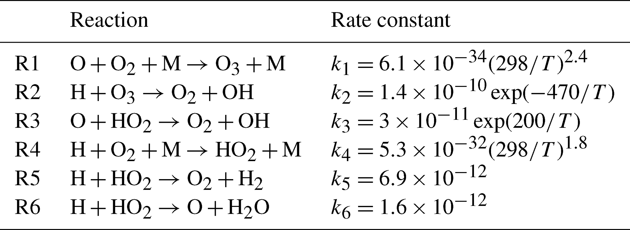
As mentioned above, the criterion for NOCE validity was proposed by Kulikov et al. (2018b). Following a minor correction by Kulikov et al. (2023b), it is expressed as follows:

$$\begin{array}{}\text{(2)}& \begin{array}{rl}\text{Crit}& \equiv {\displaystyle \frac{{\mathit{\tau }}_{{\mathrm{O}}_{\mathrm{3}}}}{{\mathit{\tau }}_{{\mathrm{O}}_{\mathrm{3}}^{\text{eq}}}}}=\mathrm{2}\cdot {\displaystyle \frac{k_{\mathrm{1}}\cdot \mathrm{M}\cdot {\mathrm{O}}_{\mathrm{2}}}{k_{\mathrm{2}}}}\cdot \left(k_{\mathrm{4}}\cdot \mathrm{M}\cdot {\mathrm{O}}_{\mathrm{2}}\cdot \left(\mathrm{1}-{\displaystyle \frac{k_{\mathrm{5}}+k_{\mathrm{6}}}{k_{\mathrm{3}}}}\right)\right.\\ & \left.+k_{\mathrm{2}}\cdot {\mathrm{O}}_{\mathrm{3}}\right)\cdot {\displaystyle \frac{\mathrm{1}}{k_{\mathrm{2}}\cdot \mathrm{H}\cdot {\mathrm{O}}_{\mathrm{3}}}}\ll \mathrm{1},\end{array}\end{array}$$

where k_i are the corresponding reaction rate constants from Table 1, ${\mathit{\tau }}_{{\mathrm{O}}_{\mathrm{3}}}$ is the ozone lifetime and ${\mathit{\tau }}_{{\mathrm{O}}_{\mathrm{3}}^{\text{eq}}}$ is the local time scale of ${\mathrm{O}}_{\mathrm{3}}^{\text{eq}}$. Calculations using a global 3D chemistry-transport model of the middle atmosphere showed that the criterion Crit=0.1 accurately defines the boundary of the region where $|{\mathrm{O}}_{\mathrm{3}}/{\mathrm{O}}_{\mathrm{3}}^{\text{eq}}-\mathrm{1}|\le \mathrm{0.1}$ (Kulikov et al., 2018b, 2023b). Moreover, Kulikov et al. (2023b) developed the theory of chemical equilibrium for a certain trace gas and provided a rigorous mathematical proof.

Since Reaction (R2) is the source of excited OH, the term $k_{\mathrm{2}}\cdot \mathrm{H}\cdot {\mathrm{O}}_{\mathrm{3}}$ in Eq. (2) can be rewritten in terms of characteristics measured by SABER using the corresponding OH(v) model:

$$\begin{array}{}\text{(3)}& k_{\mathrm{2}}\cdot \mathrm{H}\cdot {\mathrm{O}}_{\mathrm{3}}=\text{VER}/A(\mathrm{T},\mathrm{M},\mathrm{O}),\end{array}$$

where VER is the total volume emission rate of OH^∗ transitions (9→7 and 8→6) at 2.0 µm, A(T,M,O) is the function given in square brackets in Eq. (3) of Mlynczak et al. (2013a). This function is derived by combining the physicochemical balance equations for OH^∗ in the v=8 and v=9 states (see Kulikov et al., 2022b, for details):

$$\begin{array}{}\text{(4)}& \begin{array}{rl}A(\mathrm{T},\mathrm{M},\mathrm{O})& ={\displaystyle \frac{f_{\mathrm{9}}\cdot E_{\mathrm{97}}}{E_{\mathrm{9}}+B_{\mathrm{9}}\cdot {\mathrm{O}}_{\mathrm{2}}+C_{\mathrm{9}}\cdot \mathrm{O}+D_{\mathrm{9}}\cdot {\mathrm{N}}_{\mathrm{2}}}}\\ & +{\displaystyle \frac{f_{\mathrm{8}}\cdot E_{\mathrm{86}}}{E_{\mathrm{8}}+B_{\mathrm{8}}\cdot {\mathrm{O}}_{\mathrm{2}}+C_{\mathrm{8}}\cdot \mathrm{O}+D_{\mathrm{8}}\cdot {\mathrm{N}}_{\mathrm{2}}}}\\ & +{\displaystyle \frac{f_{\mathrm{9}}\cdot E_{\mathrm{86}}}{E_{\mathrm{9}}+B_{\mathrm{9}}\cdot {\mathrm{O}}_{\mathrm{2}}+C_{\mathrm{9}}\cdot \mathrm{O}+D_{\mathrm{9}}\cdot {\mathrm{N}}_{\mathrm{2}}}}\\ & \cdot {\displaystyle \frac{E_{\mathrm{98}}+B_{\mathrm{98}}\cdot {\mathrm{O}}_{\mathrm{2}}+C_{\mathrm{98}}\cdot \mathrm{O}+D_{\mathrm{98}}\cdot {\mathrm{N}}_{\mathrm{2}}}{E_{\mathrm{8}}+B_{\mathrm{8}}\cdot {\mathrm{O}}_{\mathrm{2}}+C_{\mathrm{8}}\cdot \mathrm{O}+D_{\mathrm{8}}\cdot {\mathrm{N}}_{\mathrm{2}}}},\end{array}\end{array}$$

where f_v are the nascent distributions for vibrational level v; B_v, C_v, and D_v are the total quenching coefficients for O₂, O, and N₂, respectively, for corresponding level v; E_v are the total spontaneous emission coefficients for corresponding level v; B₉₈, D₉₈, and E₉₈ are the quenching ratios for quenching by O₂, N₂, and spontaneous emission coefficients, respectively, for the transitions from level 9 to level 8. The values of these rate constants are given in Mlynczak et al. (2013a), with a correction in Mlynczak et al. (2018). Below 86–87 km, $A(\mathrm{T},\mathrm{M},\mathrm{O})\cong A(\mathrm{T},\mathrm{M},\mathrm{O}=\mathrm{0})$ due to relatively small O concentrations (Kulikov et al., 2023a). Consequently, the NOCE criterion for SABER data can be recast into a form that depends only on measurable characteristics:

$$\begin{array}{}\text{(5)}& \begin{array}{rl}\text{VER}& \ge {\text{VER}}_{\text{min}}(\mathrm{T},\mathrm{M})\equiv \mathrm{20}\cdot {\displaystyle \frac{k_{\mathrm{1}}\cdot {\mathrm{O}}_{\mathrm{2}}\cdot \mathrm{M}}{k_{\mathrm{2}}}}\cdot \left(k_{\mathrm{4}}\cdot \mathrm{M}\cdot {\mathrm{O}}_{\mathrm{2}}\right.\\ & \left.\cdot \left(\mathrm{1}-{\displaystyle \frac{k_{\mathrm{5}}+k_{\mathrm{6}}}{k_{\mathrm{3}}}}\right)+k_{\mathrm{2}}\cdot {\mathrm{O}}_{\mathrm{3}}\right)\cdot A(\mathrm{T},\mathrm{M},\mathrm{O}=\mathrm{0}),\end{array}\end{array}$$

where VER_min is the total volume emission rate at which the condition ${\mathit{\tau }}_{{\mathrm{O}}_{\mathrm{3}}}/{\mathit{\tau }}_{{\mathrm{O}}_{\mathrm{3}}^{\text{eq}}}=\mathrm{0.1}$ is satisfied. Thus, the local position of the NOCE boundary (altitude z_eq) is determined using criterion (5), where $\text{VER}={\text{VER}}_{\text{min}}(\mathrm{T},\mathrm{M})$. In the zeroth approximation (see Table 1):

$$\begin{array}{}\text{(6)}& \begin{array}{rl}{\text{VER}}_{\text{min}}& \approx \mathrm{20}\cdot {\displaystyle \frac{k_{\mathrm{1}}\cdot k_{\mathrm{4}}\cdot {{\mathrm{O}}_{\mathrm{2}}}^{\mathrm{2}}\cdot {\mathrm{M}}^{\mathrm{2}}}{k_{\mathrm{2}}}}\cdot A(\mathrm{T},\mathrm{M},\mathrm{O}=\mathrm{0})\\ & \sim {\displaystyle \frac{k_{\mathrm{1}}\cdot k_{\mathrm{4}}}{k_{\mathrm{2}}}}\sim \exp (\mathrm{470}/T)/T^{\mathrm{4.2}},\end{array}\end{array}$$

which ensures a strong anti-correlation between z_eq and temperature (Kulikov et al., 2023a): cooling of the mesopause leads to a noticeable rise in z_eq, and vice versa. Kulikov et al. (2023b) investigated the uncertainty in z_eq retrieved from SABER data. Following the standard error analysis presented, for example, in Mlynczak et al. (2013a, 2014), the uncertainty was obtained by calculating the root-sum-square of the individual sensitivities of the retrieved characteristic to perturbations in O₃, T, reaction rates, and the parameters of the A function. As a result, the uncertainty in the local altitude of the NOCE boundary was found to vary in the range of 0.1–0.3 km.

In this paper, we use the function A(T, M, O) with updated rate constants corresponding to the OH(ν) model of Panka et al. (2021). In particular, the quenching rates of OH(ν=8, 9) by O₂, N₂, and O were adopted from Adler-Golden (1997) and Caridade et al. (2013), respectively. Furthermore, the model accounts for the multiquantum quenching of OH^∗ via the process $\mathrm{OH}(\mathit{\nu }\ge \mathrm{5})+\mathrm{O}{(}^{\mathrm{3}}\text{P})\to \mathrm{OH}(\mathrm{0}\le {\mathit{\nu }}^{\prime }\le \mathit{\nu }-\mathrm{5})+\mathrm{O}{(}^{\mathrm{1}}D)$, as described by Sharma et al. (2015) and Kalogerakis et al. (2016). Applying criterion (5), we processed all simultaneous vertical profiles of p, T, O₃, and VER at geometric altitudes from the SABER database for the period 2002–2025, determining the position of the NOCE boundary as a function of time, latitude, and longitude. Additionally, the concentration of M was calculated using the ideal gas law, while the spatiotemporal distribution of the O₂ mixing ratio was adopted directly from the SABER database processing. The latitude range from 82.5° S to 82.5° N was divided into 33 bins 5° each, and all local values of z_eq falling into a given bin on a specific day of the year were averaged. Then, we calculated daily mean values of $z_{\text{eq}}^{\mathrm{d}}$ (hereafter, the superscript d denotes the daily average).

4 The connection of the NOCE boundary with spatiotemporal variability of O_x-HO_x chemistry

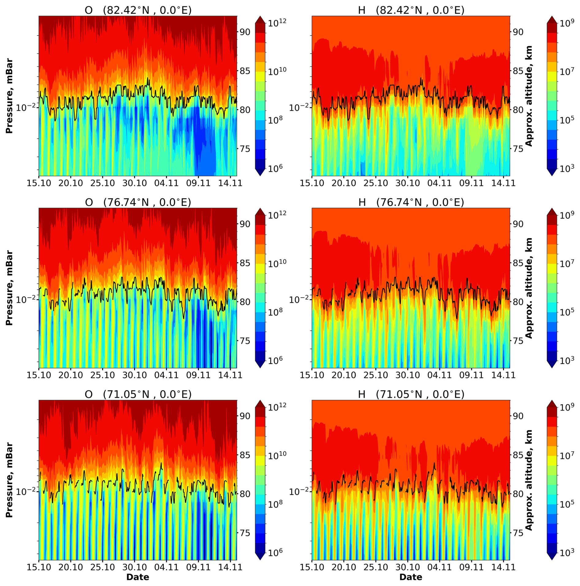
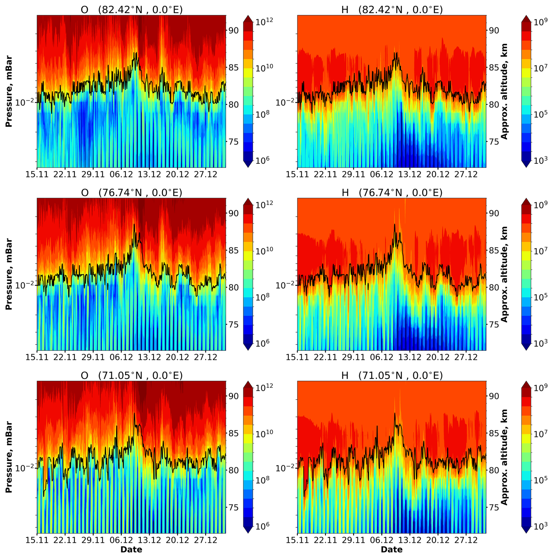
Figures 1–3 demonstrate the day-to-day evolution of O and H as a function of altitude above various northern polar locations over 3.5 months (from mid-September to December 2000), as simulated by WACCM-X. Thus, Figs. 1 and 3 correspond to periods around the autumnal equinox and the winter solstice, respectively. From mid-September to mid-October, pronounced diurnal O and H oscillations occur below 79–80 km, where nighttime values drop by several orders of magnitude relative to daytime values. These oscillations are driven by variations in solar radiation and high nighttime loss rates of HO_x and O, which are nonlinearly dependent on air concentration. Above 83–85 km, the behavior of O and H is fundamentally different. First, the diurnal range between minimum and maximum values is significantly reduced. Second, variations on multi-day timescales predominate in the corresponding spectra. The two regimes (upper and lower) of O and H oscillations are connected vertically by a transition zone several kilometers thick, which is characterized by sharp vertical gradients in the daily mean concentrations of these species. Note that the black lines in Figs. 1–3 indicate the NOCE boundary according to criterion (5). An interesting feature is observed in the dynamics of the Crit=0.1 contour line, which is typical of most nights in Fig. 1. Over the course of a single night, this line traverses the transition zone, moving from its lower part, where the strong O and H oscillations still persist, to the upper part of the transition zone, where the weak O and H oscillations are already established. Thus, as at middle and low latitudes (see Kulikov et al., 2023a), the NOCE criterion clearly indicates the local position and thickness of the transition zone. The duration of daylight decreases as the year progresses; this manifests relatively weakly in the upper region, but strongly in the lower region. Specifically, below the transition zone (see Fig. 2), the mean daily concentrations of O and H decrease noticeably, and their diurnal oscillations become less pronounced or periodically disappear (i.e., they are obscured by variations on other timescales). This is especially noticeable at 82.5° N. Finally, in December (see Fig. 3), the mean daily concentrations of O and H at lower altitudes drop to such low levels that the transition zone effectively “degenerates” into a step in the vertical profiles of these species, and the NOCE criterion marks the altitude of this transition. It should be noted that below 75 km, diurnal oscillations remain noticeable, likely due to residual photodissociation (e.g., of O₃, Fig. S1 in the Supplement) under twilight conditions. The same diurnal oscillations of O and H can be found in other runs of the WACCM-X model, e.g., https://doi.org/10.26024/5b58-nc53.

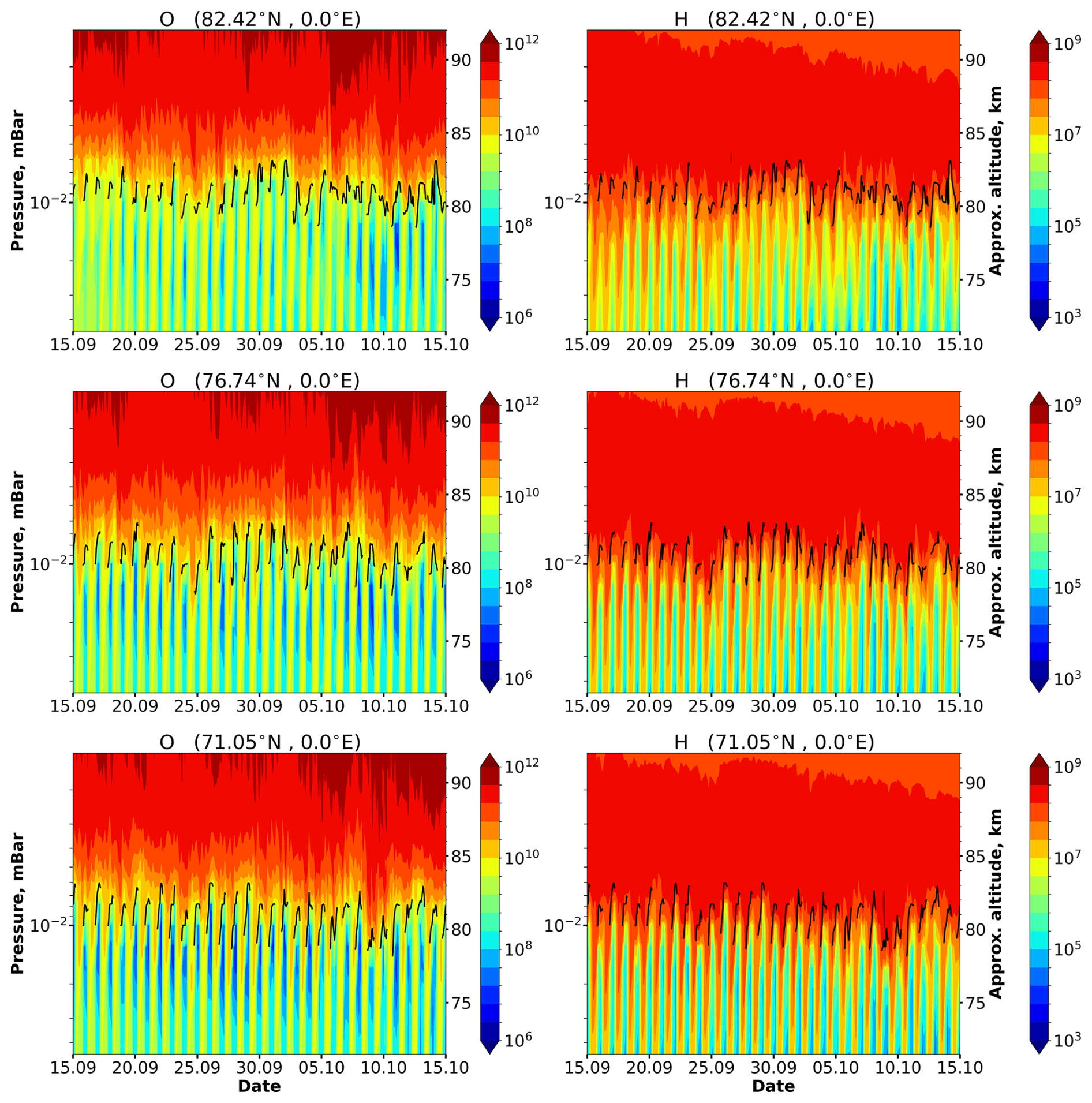
Figure 1 Time-height variations of O and H (in cm⁻³) over various polar locations in September–October 2000, calculated using the 3D chemical transport model WACCM-X. Log-pressure altitude is used as the vertical coordinate. Black lines indicate the NOCE boundary altitude based on criterion (5) (Crit=0.1).

Figure 2 The same as in Fig. 1, but in October–November 2000.

Figure 3 The same as in Fig. 1, but in November–December 2000.

5 NOCE boundary in the polar winters of 2002–2025 from SABER/TIMED data: main results and discussion

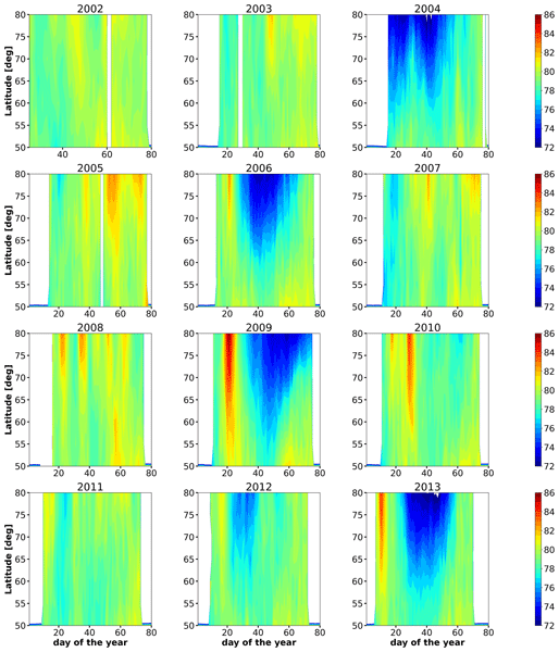
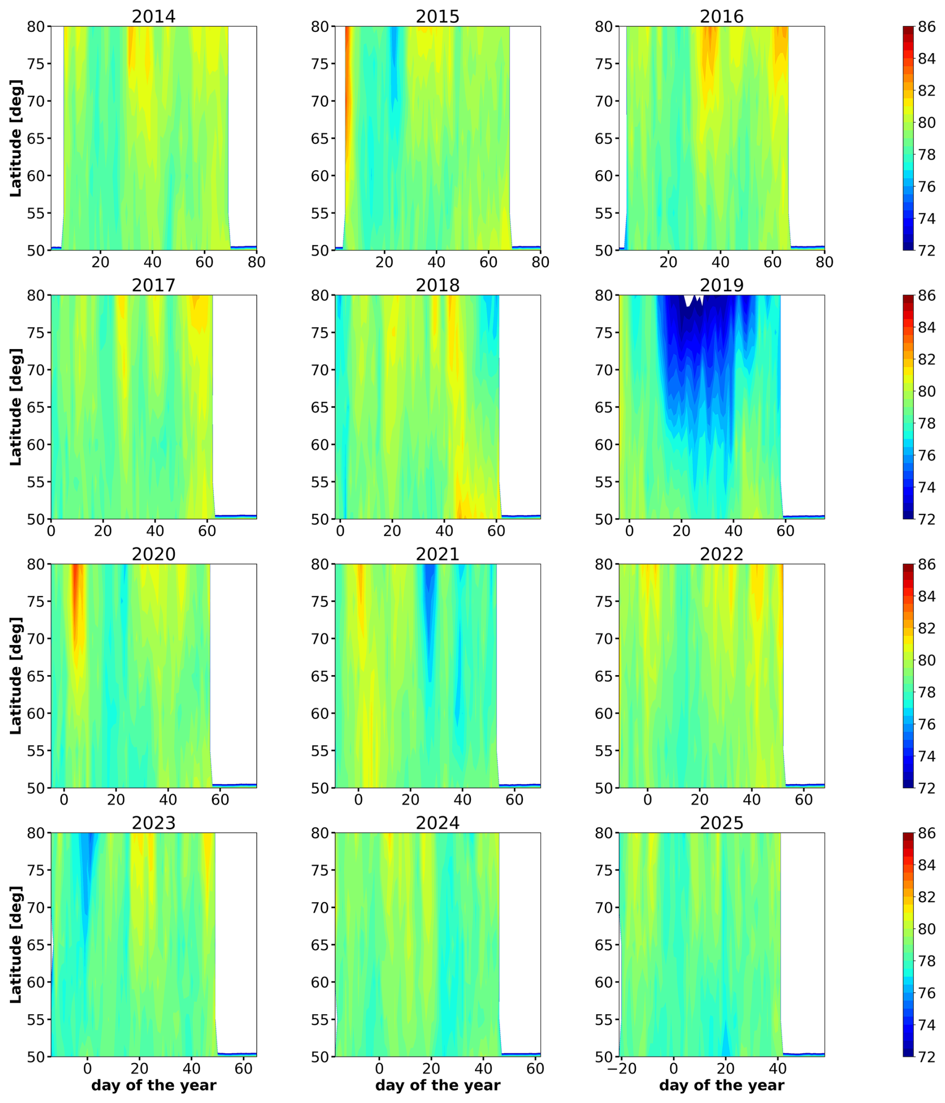
Figures 4 and 5 present contour maps showing the latitude–time evolution of $z_{\text{eq}}^{\mathrm{d}}$ in the Northern Hemisphere during the winter–spring period from 2002 to 2025, derived from SABER data. The strongest disturbances are observed in 2004, 2006, 2009, 2010, 2012, 2013, and 2019. These years are characterized by remarkable SSWs followed by elevated stratopause (ES) events. During other winters, such strong warmings did not occur; however, a notable single pulse of $z_{\text{eq}}^{\mathrm{d}}$ was observed (see, e.g., 2020), or multi-pulse behavior occurred (e.g., in 2008 and 2015). The variations in $z_{\text{eq}}^{\mathrm{d}}$ are most pronounced at 80° N and decrease toward the midlatitudes; however, in some years (e.g., 2009), they extended to 50–60° N. To identify the characteristic features of $z_{\text{eq}}^{\mathrm{d}}$ during these years and their underlying causes, we examine its time evolution at 80° N alongside the zonal mean wind at 60° N and 10 hPa (U_{60° N,10 hPa}) and the temperature difference between the pole and 60° N at 10 hPa (ΔT_{90–60° N,10 hPa}). As mentioned previously, both variables were calculated using MERRA-2 reanalysis data for the corresponding years. Furthermore, we correlate variations in $z_{\text{eq}}^{\mathrm{d}}$ with the height-time evolution of temperature in the stratosphere and mesosphere at 80° N, using data from SABER observations (Figs. S2–S5) and the JAWARA reanalysis (Yamazaki et al., 2025).

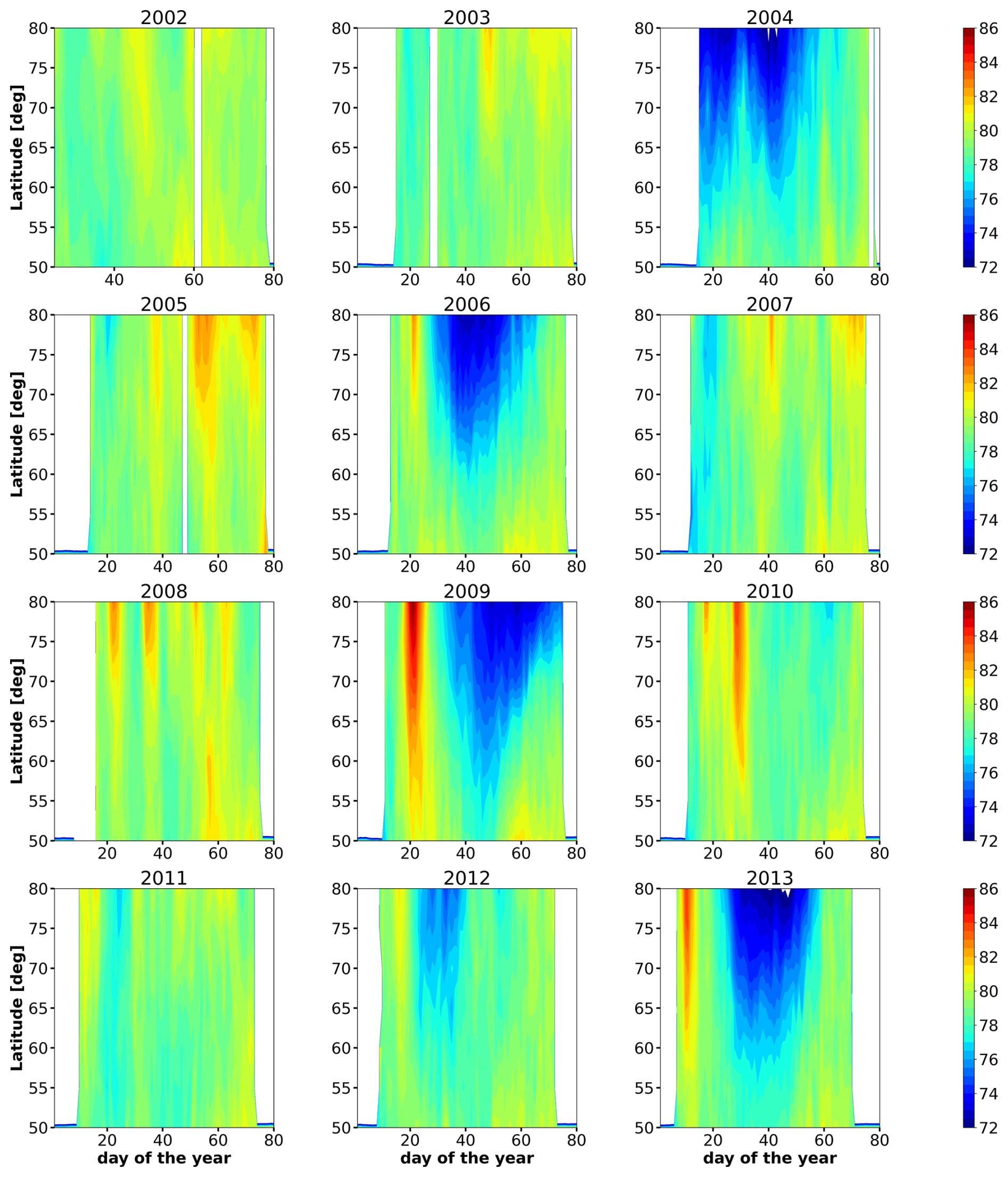
Figure 4 Latitude-time evolution of the daily mean NOCE boundary $z_{\text{eq}}^{\mathrm{d}}$ (geometrical altitude, km) at northern polar latitudes in 2002–2013 obtained from SABER data. White areas indicate missing data due to satellite geometry.

Figure 5 Same as Fig. 4, but for the period 2014–2025.

During years with ES events, a clear pattern emerges in the $z_{\text{eq}}^{\mathrm{d}}$ dynamics. We illustrate this using the winter of 2009 (Fig. 6), which featured the most intense SSW on record. In the second half of January, a pronounced pulse-like variation in $z_{\text{eq}}^{\mathrm{d}}$ was observed, during which it rapidly rose from 78 to 86 km over 5–6 d. This pulse coincided closely with the onset of the major SSW (central date: 24 January), which led to extreme cooling (up to 160 K) in the upper mesosphere and mesopause region at 80° N (Fig. S3; Fig. S10 in Yamazaki et al., 2025). From February to March, we observe: (1) an almost monotonic decrease in $z_{\text{eq}}^{\mathrm{d}}$ to 72.5 km; (2) only minor variations near this level until early March; and (3) a subsequent slow rise in $z_{\text{eq}}^{\mathrm{d}}$. According to SABER (Fig. S3) and JAWARA (Fig. S10 in Yamazaki et al., 2025) data, this behavior of $z_{\text{eq}}^{\mathrm{d}}$ in February–March can be attributed to the significant (up to 260 K) prolonged warming of the upper mesosphere at 80° N starting on 31 January during the ES event, when the stratopause ascended abruptly from ∼20–30 km to ∼82 km.

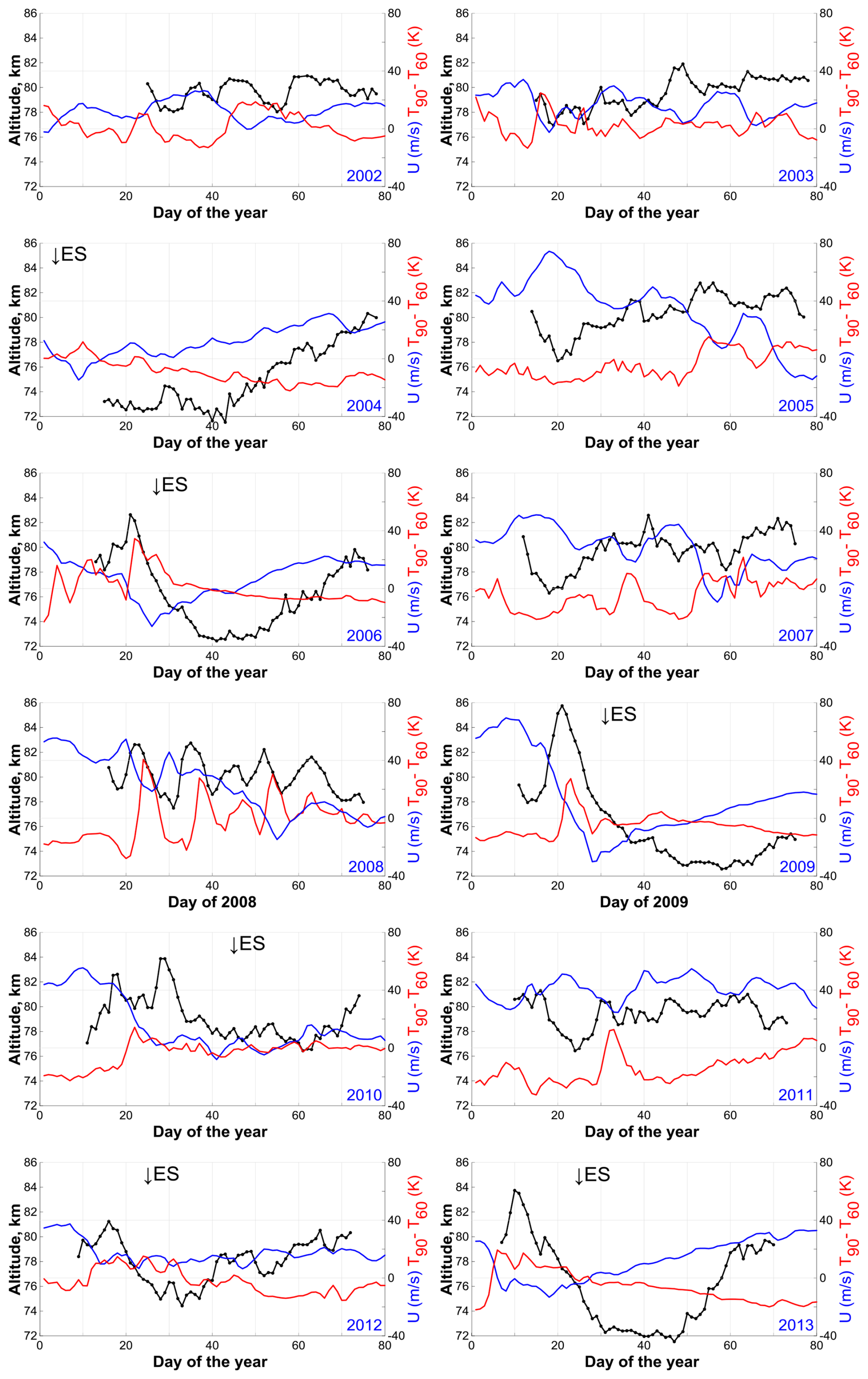
Figure 6 Time evolution of $z_{\text{eq}}^{\mathrm{d}}$ (geometrical altitude) at 80° N during 2002–2013, derived from SABER data (black lines with dots, left y-axis). Blue lines represent the zonal mean wind at 60° N and 10 hPa (right y-axis), while red lines indicate the pole-to-60° N temperature difference at 10 hPa (right y-axis); both variables are from the MERRA-2 reanalysis. The “↓ES” symbol marks the onset of the ES event in the corresponding years, as identified, for example, by Yamazaki et al. (2025).

In 2006 and 2013 (Fig. 6), the evolution of $z_{\text{eq}}^{\mathrm{d}}$ was similar to the 2009 case. SABER (Figs. S2 and S3) and JAWARA (Figs. S8 and S12 in Yamazaki et al., 2025) data indicate that the underlying mechanisms were identical. Brief upper mesospheric cooling caused by the SSW led to a pulse in $z_{\text{eq}}^{\mathrm{d}}$, while the subsequent prolonged warming during the ES event manifested as a significant decrease in $z_{\text{eq}}^{\mathrm{d}}$ to ∼72 km.

In 2004 (Fig. 6), due to SABER's satellite observation geometry, only the second stage associated with the ES is observable (Fig. S2), manifesting as a significant, prolonged decrease in $z_{\text{eq}}^{\mathrm{d}}$ to 72 km.

In 2019 (Fig. 7), the $z_{\text{eq}}^{\mathrm{d}}$ pulse was weak due to relatively mild upper mesospheric cooling, likely caused by a substantial time lag between the stratospheric warming and the zonal wind reversal. Subsequently, only a significant, prolonged decrease in $z_{\text{eq}}^{\mathrm{d}}$ below 72 km is observed, driven by the prolonged ES (Fig. S5; Fig. S15 in Yamazaki et al., 2025).

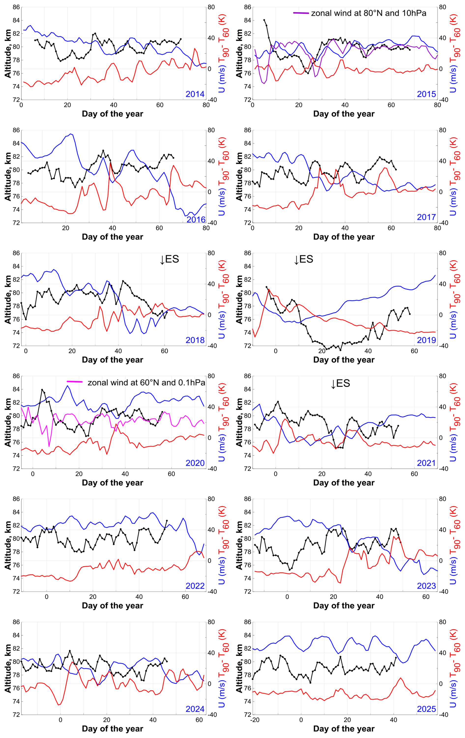
Figure 7 Same as Fig. 6, but for the period 2014–2025. Additional data in the 2015 and 2020 panels are derived from the MERRA-2 reanalysis.

In 2010, two distinct upper mesospheric cooling events occurred: one prior to the major SSW and the second during it (Fig. S3; Fig. S10 in Yamazaki et al., 2025). This resulted in a two-peaked structure in the $z_{\text{eq}}^{\mathrm{d}}$ evolution (Fig. 6). The elevated stratopause was modest in vertical extent (rising from ∼50 km to ∼70–75 km; Fig. S3) and short-lived; consequently, $z_{\text{eq}}^{\mathrm{d}}$ did not fall below 76–77 km.

The 2012 case (Fig. 6) is notable because it featured only a minor SSW (11 January), followed by an elevated stratopause. As in 2019, the $z_{\text{eq}}^{\mathrm{d}}$ pulse was muted due to relatively weak upper mesospheric cooling. The subsequent elevated stratopause (Fig. S3; Fig. S11 in Yamazaki et al., 2025), which rose from ∼35 km to ∼80–82 km, led to a drop in $z_{\text{eq}}^{\mathrm{d}}$ to ∼74 km at the end of January. This was followed by a rapid recovery of $z_{\text{eq}}^{\mathrm{d}}$ to ∼78–80 km in mid-February, coinciding with the rapid descent of the stratopause.

In 2021, the elevated stratopause was modest in vertical extent (rising from ∼50 to ∼75 km; Fig. S5; Fig. S16 in Yamazaki et al., 2025) and short-lived; consequently, $z_{\text{eq}}^{\mathrm{d}}$ did not fall below 75 km (Fig. 7).

In summary, SSWs accompanied by ES events produce a clear, two-stage pattern in $z_{\text{eq}}^{\mathrm{d}}$ evolution, characterized by fast and slow dynamics driven by the SSW and the subsequent ES, respectively. Throughout these stages, $z_{\text{eq}}^{\mathrm{d}}$ variability is governed by the magnitude and duration of the upper mesospheric cooling and warming, respectively.

As shown in Figs. 6 and 7, in years without ES events, $z_{\text{eq}}^{\mathrm{d}}$ typically varied within the 78–82 km range. Furthermore, the influence of major or minor SSWs is not clearly evident. In general, the dynamics of $z_{\text{eq}}^{\mathrm{d}}$ show no distinct regularity, nor do they exhibit a clear correlation with U_{60° N,10 hPa} or ΔT_{90–60° N,10 hPa}. This is particularly noticeable in years with a relatively weak polar vortex (e.g., 2002, 2003, 2014, 2021, and 2024). However, three notable exceptions are evident in 2008, 2015, and 2020.

In 2008 (Fig. 6), $z_{\text{eq}}^{\mathrm{d}}$ exhibited pronounced quasi-periodic oscillations with a period of approximately 7–10 d at altitudes between 77 and 83 km. Five distinct maxima in the NOCE boundary height are observed on 23 January, 3 February, 14 February, 21 February, and 3 March. Wang and Alexander (2009) identified four SSW events during this period: three consecutive minor SSWs and one major event, occurring on 25 January, 2 February, 16 February, and 23 February, respectively. The height–time temperature evolution derived from SABER observations (Fig. S3) indicates that these SSWs induced quasi-periodic temperature oscillations at 80° N above 70 km, with minima coinciding with the SSW events. As shown in Sect. 3, the NOCE boundary is strongly sensitive to temperature. Notably, these temperature oscillations are consistent with JAWARA reanalysis data (Fig. S9 in Yamazaki et al., 2025). Thus, the first four $z_{\text{eq}}^{\mathrm{d}}$ oscillations can be attributed to the SSWs, whereas the fifth may be a manifestation of the seasonal restructuring of stratospheric dynamics, characterized by oscillations of the mean zonal wind about zero (Wang and Alexander, 2009).

In 2015, due to the SABER satellite measurement geometry, the evolution of $z_{\text{eq}}^{\mathrm{d}}$ began with a sharp drop from 84 to 78 km (Fig. 7). Manney et al. (2015) noted that this winter was characterized by an unusual minor SSW in early January, which exerted an impact on atmospheric dynamics comparable to that of a major SSW. During this period, the zonal wind at 10 hPa reversed above 70° N, a reversal that lasted for only a few days (purple line in Fig. 7). Consistent with this, a drop in the stratopause was observed, accompanied by brief cooling at 80° N above 75 km, as indicated by SABER and JAWARA data; see Fig. S4 in the Supplement and S13 in Yamazaki et al. (2025). Thus, the initial $z_{\text{eq}}^{\mathrm{d}}$ maximum (84 km) at 80° N during this period can be attributed to this SSW. Notably, this maximum extended from the pole down to 55–60° N (Fig. 5). The subsequent strengthening and reconfiguration of the polar vortex later in January led to mesopause warming and a further decrease in $z_{\text{eq}}^{\mathrm{d}}$ to below 78 km.

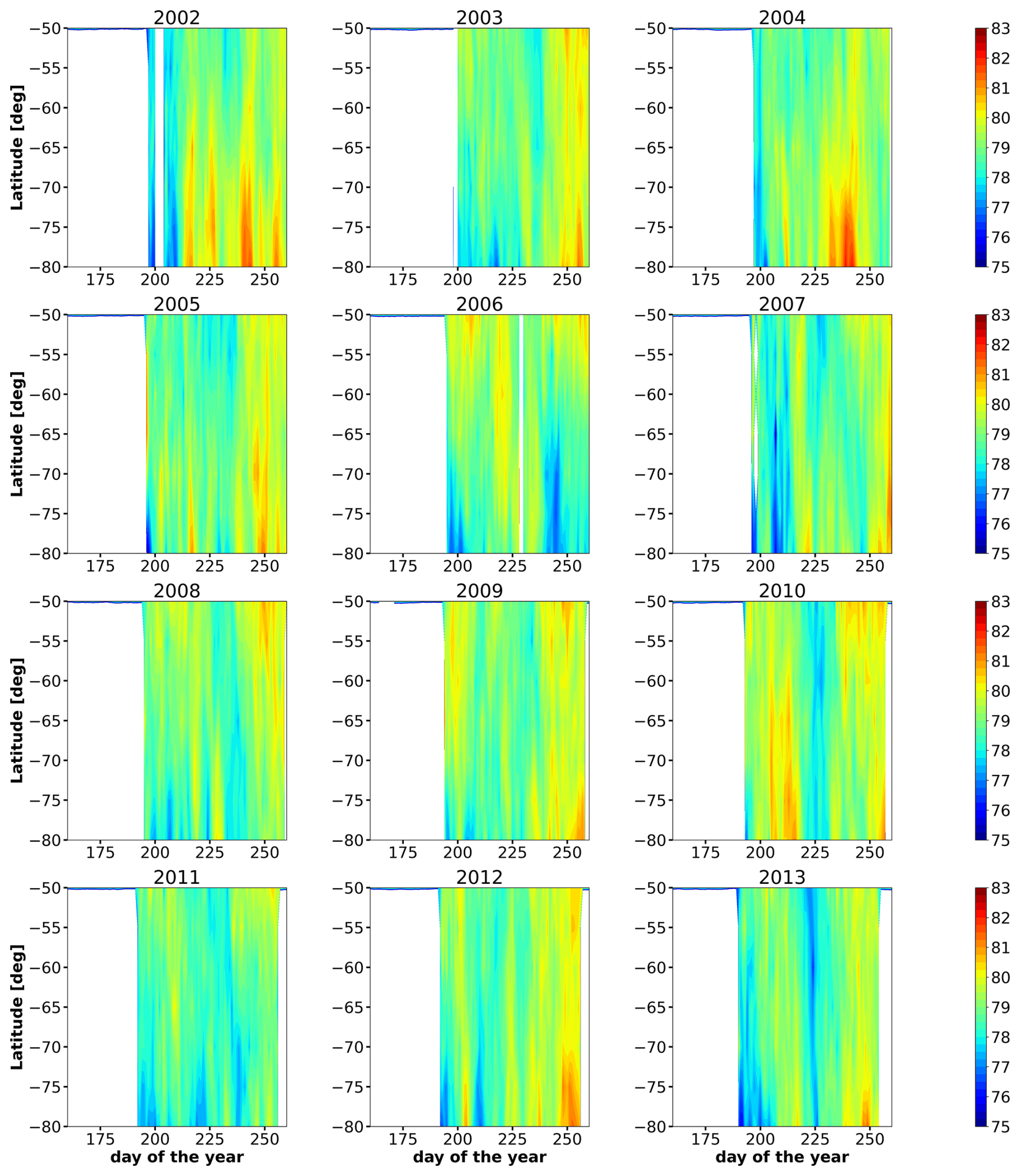
Figure 8 Latitude-time evolution of the daily mean NOCE boundary $z_{\text{eq}}^{\mathrm{d}}$ (geometrical altitude, km) at southern polar latitudes in 2002–2013 obtained from SABER data. White areas indicate missing data due to satellite geometry.

Over a two-week period in January 2020 (Fig. 7), a pronounced pulse-like variation in $z_{\text{eq}}^{\mathrm{d}}$ was observed, during which it rose from 78 to 84 km before returning to its original level. According to Lawrence et al. (2020) and Lukianova et al. (2021), this winter was characterized by a remarkably strong stratospheric polar vortex, driven by unusually weak tropospheric wave activity and wave reflection in the polar upper stratosphere. During the first 10 d of January 2020, a latitudinal and altitudinal splitting of the polar vortex occurred. This was accompanied by periodic accelerations in the zonal wind, causing a drop and warming of the stratopause, a zonal wind reversal at mesospheric altitudes (purple line in Fig. 7), and mesopause cooling with the formation of a temperature inversion layer (Lukianova et al., 2021). The mesopause cooling can be seen in Fig. S5 in the Supplement and Fig. S15 in Yamazaki et al. (2025). This event was not a typical SSW driven by planetary wave breaking. The subsequent strengthening and reconfiguration of the vortex later in January led to mesopause warming and the dissipation of the inversion layer. Thus, the pulse-like variation in $z_{\text{eq}}^{\mathrm{d}}$ was a manifestation of the intrinsic dynamics of the polar vortex, rather than a classical warming event driven by the breaking of upward-propagating planetary waves.

In summary, SSWs without an ES, as well as the internal dynamics of the polar vortex, can lead to pronounced variations in $z_{\text{eq}}^{\mathrm{d}}$ provided such events are accompanied by significant local cooling in the upper mesosphere.

Figures 8 and 9 present contour maps showing the southern latitude–time evolution of $z_{\text{eq}}^{\mathrm{d}}$ in the Southern Hemisphere from June to September between 2002 and 2025, derived from SABER data. Compared to the Northern Hemisphere maps in Figs. 4 and 5, significantly weaker $z_{\text{eq}}^{\mathrm{d}}$ variations are observed. The strongest disturbances occurred poleward of 60° S during the winters of 2002, 2004, 2012, 2014, 2017, and 2023. Figure 10 shows typical examples of $z_{\text{eq}}^{\mathrm{d}}$ time evolution at 80° S for selected years, derived from SABER data.

Figure 9 Same as Fig. 8, but for the period 2014–2025.

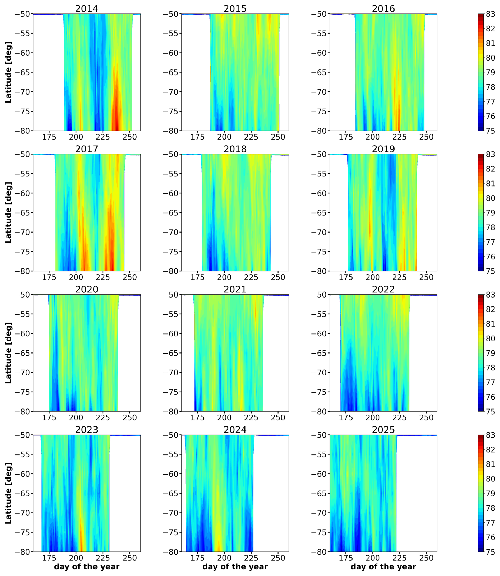
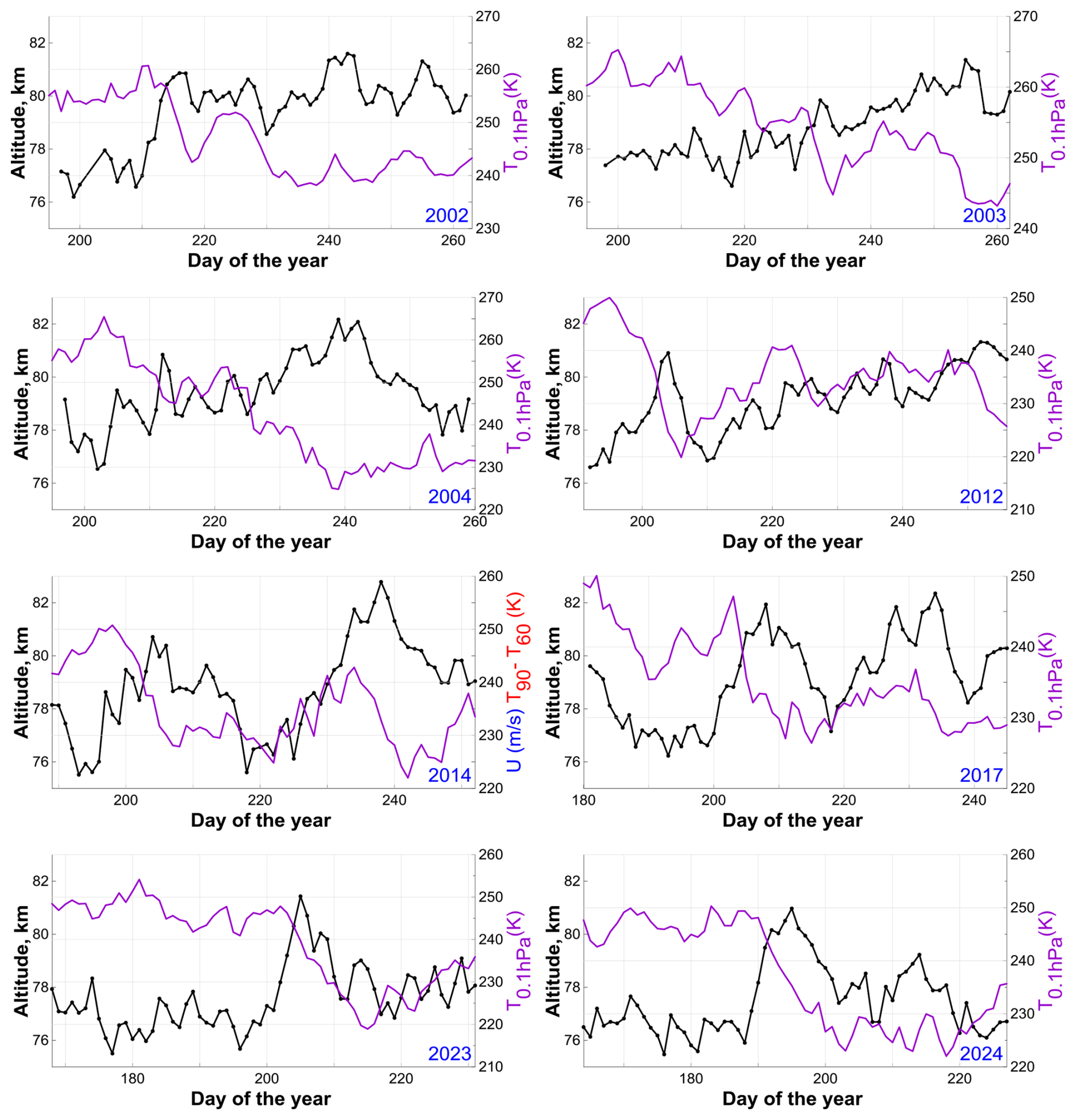
Figure 10 Time evolution of $z_{\text{eq}}^{\mathrm{d}}$ (geometrical altitude) at 80° S (black lines with dots, left y-axis), derived from SABER data for the selected years. Purple lines represent the zonal mean temperature at 60° S and 0.1 hPa (right y-axis) from the MERRA-2 reanalysis.

Note that the central dates of most Southern Hemisphere SSWs fall outside the time intervals when SABER's orbital geometry permits the determination of $z_{\text{eq}}^{\mathrm{d}}$ poleward of 55° S. In particular, the SSWs of 2002 and 2019 both occurred in September. According to Vincent et al. (2022), the central dates of the minor SSWs between 2002 and 2019 that were captured by SABER measurements were 23 August 2002 (day 235), 2 September 2002 (day 245), 13 September 2002 (day 256), 6 August 2008 (day 218), 2 August 2010 (day 214), 20 August 2012 (day 233), and 7 September 2013 (day 250). Only weak manifestations of these events are visible in the $z_{\text{eq}}^{\mathrm{d}}$ evolution shown in Figs. 8–10. Furthermore, Zi et al. (2025) reported that the central dates of the two minor SSWs in 2024 were 13 July 2024 (day 195) and 4 August 2024 (day 217). Figure 10 (the panel for 2024) shows that the first event corresponded to a local $z_{\text{eq}}^{\mathrm{d}}$ rise from ∼77 to ∼82 km, whereas the second did not significantly perturb $z_{\text{eq}}^{\mathrm{d}}$.

The time evolution of $z_{\text{eq}}^{\mathrm{d}}$ at 80° S can be classified into four distinct types: (1) monotonic growth (e.g., 2003); (2) a step-like change (e.g., 2002) or a change in slope (e.g., 2004); (3) a pulse-like disturbance (e.g., 2012, 2023, 2024); and (4) quasi-periodic oscillations with a period of ∼20–30 d (e.g., 2014, 2017). A comparison with MERRA-2 temperature data at 60° S and 0.1 hPa (T_{60° S,0.1 hPa}), shown in Fig. 10, indicates that many features of the $z_{\text{eq}}^{\mathrm{d}}$ evolution can be explained by intrinsic mesospheric dynamics. In particular, the step-like change in $z_{\text{eq}}^{\mathrm{d}}$ in 2002 and the pulse in 2023 were accompanied by similar variations in T_{60° S,0.1 hPa}. The monotonic growth of $z_{\text{eq}}^{\mathrm{d}}$ in 2003 corresponded to gradual cooling of the lower mesosphere, while the change in slope in 2004 exhibited a strong anticorrelation (correlation coefficient of $\sim -\mathrm{0.8}$) with T_{60° S,0.1 hPa}. Furthermore, the lower mesospheric temperature in 2017 also displayed quasi-periodic oscillations with a period closely matching that of the $z_{\text{eq}}^{\mathrm{d}}$ oscillations.

In summary, $z_{\text{eq}}^{\mathrm{d}}$ variations at southern polar latitudes during winter are significantly weaker than those at northern latitudes. These variations are generally decoupled from SSWs and can instead be attributed to intrinsic mesospheric dynamics.

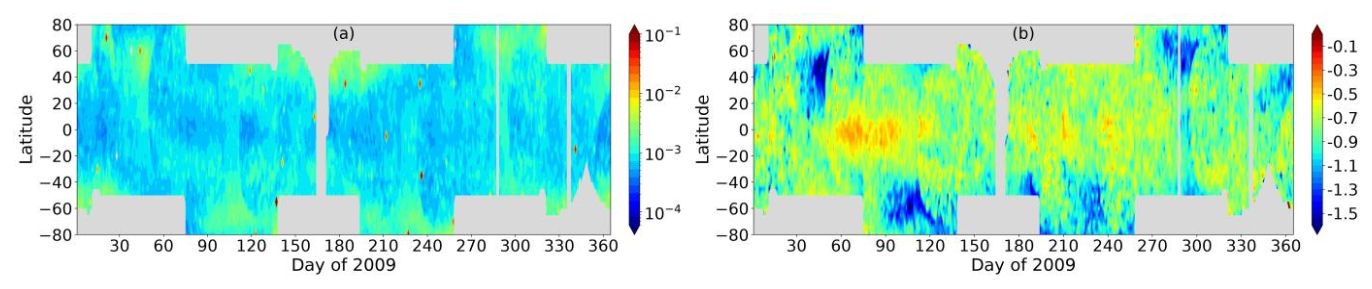
Figure 11 (a) The difference (in km) between $z_{\text{eq}}^{\mathrm{d}}$ values at 80° N derived from 2009 SABER data, assuming O=0 and O≠0. (b) The difference (in km) between $z_{\text{eq}}^{\mathrm{d}}$ values derived from 2009 SABER data using the new and previous rate constants for function A.

6 Discussion

We now show that the sharp change in the diurnal oscillations of O and H above 80 km (discussed in Sect. 4) is caused by the strong altitude dependence of their nighttime chemical lifetimes. The main loss processes for O at these altitudes are the reactions $\mathrm{O}+\mathrm{OH}\to {\mathrm{O}}_{\mathrm{2}}+\mathrm{H}$ and $\mathrm{O}+{\mathrm{HO}}_{\mathrm{2}}\to {\mathrm{O}}_{\mathrm{2}}+\mathrm{OH}$, whereas the main loss processes for H are the reactions $\mathrm{H}+{\mathrm{HO}}_{\mathrm{2}}\to {\mathrm{O}}_{\mathrm{2}}+{\mathrm{H}}_{\mathrm{2}}$ and $\mathrm{H}+{\mathrm{HO}}_{\mathrm{2}}\to \mathrm{O}+{\mathrm{H}}_{\mathrm{2}}\mathrm{O}$ (Kulikov et al., 2023b). Kulikov et al. (2023a), based on the equations describing purely chemical O and H nighttime evolution, evaluated the nighttime lifetimes of O and H:

$$\begin{array}{}\text{(7)}& {\displaystyle }\begin{array}{rl}{\mathit{\tau }}_{\mathrm{O}}& \equiv {\displaystyle \frac{\mathrm{O}}{|\mathrm{d}\mathrm{O}/\mathrm{d}t|}}={\displaystyle \frac{\mathrm{1}}{\mathrm{2}\cdot k_{\mathrm{4}}\cdot \mathrm{M}\cdot {\mathrm{O}}_{\mathrm{2}}}}\cdot {\left({\displaystyle \frac{\mathrm{O}}{\mathrm{H}}}\right)}_{\text{lt}={\text{lt}}_{\mathrm{n}}}\\ & -\left(\mathrm{1}-{\displaystyle \frac{k_{\mathrm{5}}+k_{\mathrm{6}}}{k_{\mathrm{3}}}}\right)\cdot (\text{lt}-{\text{lt}}_{\mathrm{n}}),\end{array}\end{array}$$

$$\begin{array}{}\text{(8)}& {\displaystyle }\begin{array}{rl}{\mathit{\tau }}_{\mathrm{H}}& \equiv {\displaystyle \frac{\mathrm{H}}{|\mathrm{d}\mathrm{H}/\mathrm{d}t|}}={\displaystyle \frac{\mathrm{1}}{\mathrm{2}\cdot k_{\mathrm{4}}\cdot \mathrm{M}\cdot {\mathrm{O}}_{\mathrm{2}}}}\cdot {\displaystyle \frac{k_{\mathrm{3}}}{k_{\mathrm{5}}+k_{\mathrm{6}}}}\cdot {\left({\displaystyle \frac{\mathrm{O}}{\mathrm{H}}}\right)}_{\text{lt}={\text{lt}}_{\mathrm{n}}}\\ & -\left({\displaystyle \frac{k_{\mathrm{3}}}{k_{\mathrm{5}}+k_{\mathrm{6}}}}-\mathrm{1}\right)\cdot (\text{lt}-{\text{lt}}_{\mathrm{n}}),\end{array}\end{array}$$

where lt is the local time, lt_n is the onset of night, $(\frac{\mathrm{O}}{\mathrm{H}}{)}_{\text{lt}={\text{lt}}_{\mathrm{n}}}$ is the $\mathrm{O}/\mathrm{H}$ ratio at the onset of night. Note that $k_{\mathrm{3}}\gg k_{\mathrm{5}}+k_{\mathrm{6}}$ (see Table 1). Above the NOCE boundary: ${\mathrm{O}}_{\mathrm{3}}\approx {\mathrm{O}}_{\mathrm{3}}^{\text{eq}}=\frac{k_{\mathrm{1}}\cdot \mathrm{O}\cdot {\mathrm{O}}_{\mathrm{2}}\cdot \mathrm{M}}{k_{\mathrm{2}}\cdot \mathrm{H}}$, then $(\frac{\mathrm{O}}{\mathrm{H}}{)}_{\text{lt}={\text{lt}}_{\mathrm{n}}}=\frac{({\mathrm{O}}_{\mathrm{3}}{)}_{\text{lt}={\text{lt}}_{\mathrm{n}}}}{{\mathrm{M}}^{\mathrm{2}}}$. Moreover, in the transition zone, the ozone volume mixing ratio (${\mathrm{O}}_{\mathrm{3}}/\mathrm{M}$) begins to increase, forming a secondary maximum at 90–95 km. This means that the first terms in Eqs. (7) and (8) increase with altitude faster than M⁻³, leading to approximately the same altitude dependence for τ_O and τ_H. Thus, the lower regime of O and H evolution, characterized by strong diurnal oscillations, corresponds to the condition ${\mathit{\tau }}_{\mathrm{O},\mathrm{H}}\ll D_{\mathrm{n}}$, where D_n is the duration of the night, whereas the weak diurnal oscillations of O and H at higher altitudes correspond to the opposite condition: ${\mathit{\tau }}_{\mathrm{O},\mathrm{H}}\gg D_{\mathrm{n}}$. Consequently, the existence of a narrow transition zone connecting the two regimes of O and H oscillations is due to a sharp increase in their lifetimes with increasing altitude.

In the ozone equilibrium approximation, criterion (5) can be rewritten as follows:

$$\begin{array}{}\text{(9)}& \begin{array}{rl}\text{Crit}=\mathrm{2}& \cdot \left(k_{\mathrm{4}}\cdot \mathrm{M}\cdot {\mathrm{O}}_{\mathrm{2}}\cdot \left(\mathrm{1}-{\displaystyle \frac{k_{\mathrm{5}}+k_{\mathrm{6}}}{k_{\mathrm{3}}}}\right)+k_{\mathrm{2}}\cdot {\mathrm{O}}_{\mathrm{3}}\right)\\ & \cdot {\displaystyle \frac{\mathrm{1}}{k_{\mathrm{2}}\cdot \mathrm{O}}}\le \mathrm{0.1}.\end{array}\end{array}$$

It can be seen that the Crit=0.1 contour corresponds to the following expression:

$$\begin{array}{}\text{(10)}& k_{\mathrm{2}}\cdot \mathrm{O}=\mathrm{20}\cdot \left(k_{\mathrm{4}}\cdot \mathrm{M}\cdot {\mathrm{O}}_{\mathrm{2}}\cdot \left(\mathrm{1}-{\displaystyle \frac{k_{\mathrm{5}}+k_{\mathrm{6}}}{k_{\mathrm{3}}}}\right)+k_{\mathrm{2}}\cdot {\mathrm{O}}_{\mathrm{3}}\right),\end{array}$$

which implies that the position of the NOCE boundary is closely tied to a particular value of the atomic oxygen concentration. Note that the product $k_{\mathrm{4}}\cdot \mathrm{M}\cdot {\mathrm{O}}_{\mathrm{2}}$ is the dominant term of this relation, which also determines the lifetimes of O and H in Eqs. (7) and (8). As can be seen from Fig. 1, at the beginning of the night, the NOCE boundary lies in the region exhibiting strong diurnal O oscillations. However, since the O concentration at these altitudes drops by 1–2 orders of magnitude or more during the night, the NOCE boundary, according to Eq. (10), must inevitably rise to those altitudes where a high O concentration persists at the end of the night, i.e., in the region of weak diurnal variations of this component. This is why, during each night, the Crit=0.1 contour cuts through the transition zone, passing from its lower part to the upper one, and clearly captures its main features (local position and thickness).

In this paper, we determined the NOCE boundary altitude, z_eq, using the function A(T, M, O) in Eq. (5) with new rate constants corresponding to the OH(v) model of Panka et al. (2021). We carried out an additional analysis to verify the approximation $A(\mathrm{T},\mathrm{M},\mathrm{O})\cong A(\mathrm{T},\mathrm{M},\mathrm{O}=\mathrm{0})$ at the NOCE boundary. For this purpose, we calculated z_eq in two ways: assuming O=0 and O≠0. In the latter case, the atomic oxygen concentration was determined from Eqs. (1) and (3) using the ozone equilibrium condition (${\mathrm{O}}_{\mathrm{3}}={\mathrm{O}}_{\mathrm{3}}^{\text{eq}}$), following Mlynczak et al. (2013a). Figure 11a shows the difference in z_eq values for 2009 as an example. Irrespective of latitude and season, the difference is generally less than 0.01 km, with very rare deviations of up to 0.1–0.2 km, which demonstrates the validity of this approximation. In addition, we compared the z_eq values determined using the new rate constants for function A with those derived using the previous rate constants (Mlynczak et al., 2013a, 2018). We found that the new rate constants led to a systematic downward shift in z_eq of approximately 0.5–1.5 km (Fig. 11b). Thus, our method for determining the NOCE boundary position is relatively insensitive to the choice of OH^∗ model parameters, demonstrating its robustness.

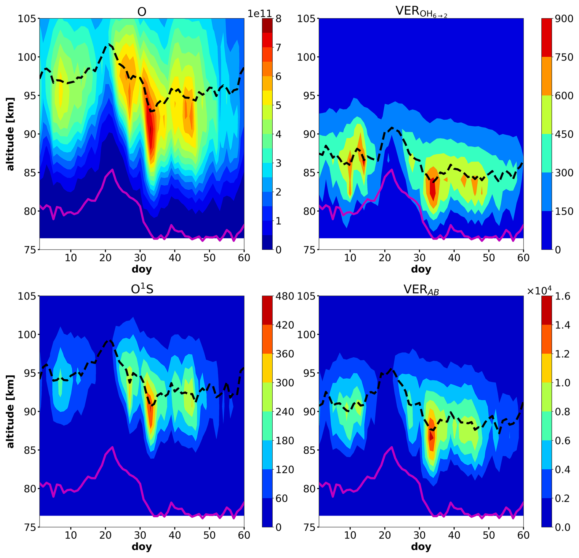
Figure 12 Time evolution of the daily zonal mean profiles (in geometrical altitude) of O (in cm⁻³) and the volume emission rate (in photon cm⁻³ s⁻¹) of OH(6-2), O(¹S) at 557.7 nm, and O₂(b${}^{\mathrm{1}}{\mathrm{\Sigma }}_g^{+}$) at 762 nm (Atmospheric Band) at ∼80° N during January–February 2009, simulated using the Canadian Middle Atmosphere Model (CMAM). The black dashed lines indicate the medians of the respective vertical distributions, while the magenta line marks the daily zonal mean NOCE boundary.

The analysis presented in Sect. 5 shows that the most pronounced variability of the NOCE boundary at high northern latitudes occurs during and after strong SSWs with subsequent elevated stratopause events. Just prior to or directly during such warmings, the daily mean boundary near the North Pole can rise abruptly to 86 km, and local values may reach even higher altitudes, up to 90–91 km. This implies that during these periods, retrieval methods for sparsely measured mesopause characteristics (in particular, atomic oxygen, O) that rely on the ozone equilibrium condition may yield significant unquantified errors at altitudes below this level due to the breakdown of the equilibrium. Conversely, immediately after such SSWs (during the ES stage), the NOCE boundary rapidly descends to 72–74 km and can remain at these altitudes for an extended period. Thus, during an ES event, the altitude range over which the ozone equilibrium condition is well satisfied is significantly expanded, allowing for the reliable retrieval of O and other characteristics well below 80 km.

The 2009 event (Fig. 6) demonstrates the most pronounced variations in $z_{\text{eq}}^{\mathrm{d}}$, particularly during the major SSW that triggered the $z_{\text{eq}}^{\mathrm{d}}$ pulse. A number of studies (e.g., Gao et al., 2011; Medvedeva et al., 2019; Hu et al., 2025) indicate strong perturbations in chemical constituents (specifically, atomic oxygen) and airglow emissions in the mesopause region during both this specific SSW and other major SSWs accompanied by an elevated stratopause. To identify common patterns in the evolution of the NOCE boundary and these characteristics, we examined multiple datasets from various 3D models for 2009 to find one that reproduced the same pulse-like variation in the NOCE boundary during this event. First, we found that the WACCM-X data were unsuitable for this purpose. A likely reason is that the WACCM-X temperature data show a remarkably weaker cooling of the upper mesosphere during this SSW compared to the SABER data, as can be seen by comparing Fig. 1a in Hu et al. (2025) with Fig. S3 for 2009. Second, the temperatures from the 2009 annual run of the Canadian Middle Atmosphere Model (CMAM; Scinocca et al., 2008), with 6-hourly output provided by the Canadian Centre for Climate Modelling and Analysis, correspond much better to the SABER data (e.g., Shepherd et al., 2014). We used this run to calculate the daily zonal mean evolution of the NOCE boundary at ∼80° N (Fig. 12), alongside the daily zonal mean vertical profiles of O and the volume emission rates of OH(6-2), O(¹S) at 557.7 nm, and O₂(b${}^{\mathrm{1}}{\mathrm{\Sigma }}_g^{+}$) at 762 nm (Atmospheric Band). To achieve this, the distributions of OH(v=1–9), O(¹S), and O₂(b${}^{\mathrm{1}}{\mathrm{\Sigma }}_g^{+}$) were calculated using established airglow models driven by CMAM profiles of pressure, temperature, and relevant chemical species (O, H, O₂, and O₃). Specifically, the OH(v=1–9) distributions were derived using the model by Panka et al. (2021; see their Table 1 for details), assuming vibrational level equilibrium. The O(¹S) distributions were calculated using the McDade et al. (1986) approximation, with rate constants updated by Gao et al. (2012). Finally, the O₂(b${}^{\mathrm{1}}{\mathrm{\Sigma }}_g^{+}$) distributions were modeled following Grygalashvyly et al. (2021), utilizing the aforementioned OH(v=1–9) profiles alongside the standard CMAM atmospheric profiles. As shown in Fig. 12, the NOCE boundary closely follows the variability of the medians of vertical distributions of O and the airglow emissions. Thus, we can propose that the NOCE boundary can serve as an indicator of disturbances in O_x–HO_x chemistry and the associated airglow variations arising during such powerful SSWs in the mesopause region.

7 Conclusions

At polar latitudes, the NOCE criterion clearly indicates the local position and thickness of the transition zone separating pronounced and weak photochemical oscillations of O and H caused by the diurnal variations in solar radiation. This is due to the strong dependence of the NOCE boundary position on the altitude of the layer with a relatively high O concentration. During the polar night, the transition zone effectively “degenerates” into a sharp step in the vertical profiles of these components, and the NOCE criterion identifies the altitude of this step.

Based on SABER observations (Figs. 4–7), the most pronounced variability of the NOCE boundary at northern polar latitudes is observed during and after strong SSWs followed by stratopause elevation events. Just prior to or directly during such warmings, the daily mean altitude of the boundary near the North Pole can jump to 86 km, while local values can be even higher, up to 90–92 km. Immediately after such SSWs, the NOCE boundary rapidly descends to 72–74 km and can remain there for an extended period. Thus, the altitude range where the ozone equilibrium condition is valid for determining O and other mesopause characteristics changes significantly during such events.

Model studies of the winter of 2009 show that the NOCE boundary closely tracks the variability of the medians of the vertical distributions of O and volume emission rates of OH(v=1–9), O(¹S), and O₂(b${}^{\mathrm{1}}{\mathrm{\Sigma }}_g^{+}$).

At southern polar latitudes, variations in the NOCE boundary values during winter are significantly weaker than at northern latitudes. These variations are generally unrelated to minor SSWs during these years, but can instead be explained by the dynamics of the polar vortex in the lower mesosphere.