CO emissions and NO_x ∕ CO ratios from the extreme 2025 Iberian wildfires: TROPOMI-based estimates and comparison with inventories

In summer 2025 the Iberian Peninsula experienced exceptional wildfire activity, with nearly 0.5 Mha of land burned and carbon emissions that broke European records since 2003. In this work, we quantify CO emission rates from 15 wildfires in northwestern Spain and northern Portugal during August 2025 using satellite observations from the Tropospheric Monitoring Instrument (TROPOMI). Through a plume masking method that exploits the synergy between collocated NO₂ and CO TROPOMI observations in complex multi-fire scenes, we infer CO emission rates for 46 individual hotspots. The area studied represents about 70 % of the total burned area in the Iberian Peninsula during that period. The inferred TROPOMI-based emission rates are compared against three fire emission inventories: the Global Fire Assimilation System (GFAS), the Global Fire Emissions Database (GFED) and the Fire Inventory from NCAR (FINN). Our results indicate that inventories systematically underestimate CO emissions by about a factor of 3 relative to TROPOMI-derived estimates, consistent with findings from previous studies on other extreme wildfire events. Additionally, we also investigate the NO_x $/$ CO mole density ratio (MDR; NO_x= NO + NO₂) as a proxy for combustion efficiency. This estimate is obtained from TROPOMI NO₂ $/$ CO MDR using literature-based NO₂-to-NO_x conversion factor. The TROPOMI-derived NO_x $/$ CO MDR values are consistently lower than those from inventories, with regional variability suggesting differences in combustion phase and fuel type across the study domain. These results highlight the potential of combined satellite observations to assess wildfire emissions in complex fire scenes, while also pointing to limitations in current fire emission inventories under such conditions.

1 Introduction

Wildfires are recurrent phenomena across terrestrial ecosystems with effects depending on the spatial extent and intensity of the fire and the characteristics of the affected area. Wildfires can lead to loss of vegetation and biodiversity, soil degradation, damage to infrastructure, health issues and casualties. Thus, wildfires are of environmental and socio-economic concern (Bowman et al., 2009; Moritz et al., 2014; Agbeshie et al., 2022; Chen et al., 2024). Regarding atmospheric and climate effects, wildfires degrade air quality, perturb atmospheric chemistry and disturb the carbon cycle. Biomass burning emissions include gases and aerosols, such as CO₂, CO, CH₄, NO_x (NO + NO₂), volatile organic compounds (VOCs), black carbon and fine particulate matter (PM_2.5), which affect human health, atmospheric oxidizing capacity, ozone formation and radiative forcing (Andreae and Merlet, 2001; Kaiser et al., 2012; Mao et al., 2013; Voulgarakis and Field, 2015; Andreae, 2019).

The magnitude and atmospheric impact of these emissions depend strongly on fuel properties, combustion conditions and meteorology. Wildfires can produce highly variable and sometimes exceptionally large emission events. These large wildfires (≥ 500 ha) occur every year in many prone regions worldwide (Doerr and Santín, 2016; Kelley et al., 2025). Climate change, together with fuel accumulation, change of land use and human ignitions, is favoring conditions for extreme wildfires, with recent events characterized by exceptional intensities and spreads of extraordinary scale and impact (Duane et al., 2021; Abatzoglou et al., 2025; Quaye et al., 2026). The 2019/2020 Australian fires are an example of such extreme events, not only for their ecological impact and estimated emissions equivalent to about 195 Tg of carbon (TgC), but also for their exceptional pyroconvective activity, which injected large amounts of smoke and water vapor into the stratosphere (Khaykin et al., 2020; van der Velde et al., 2021). Another record-breaking wildfire took place in 2023 over Canada, with nearly 15 Mha burned and over 640 TgC emitted to the atmosphere (Byrne et al., 2024; Jain et al., 2024; Zhang et al., 2025). Similarly, the 2024–2025 South American fire season accounted for more than 10 Mha burned just in Bolivia and 501 TgC emitted from Brazil and Bolivia's fires (Bourgoin et al., 2025; Kelley et al., 2025). The European continent is also prone to large wildfires, with the fire season expanding from June to September when, particularly countries within the Mediterranean Basin such as Portugal, Spain, Italy, Cyprus, Türkiye or Greece, suffer from large wildfires. The latest European State of the Climate report (C3S/ECMWF and WMO, 2026) indicated that fire danger (Zacharakis and Tsihrintzis, 2023) across Europe during summer 2025 was above the 1991–2020 average. The same report identified 2025 as record year for burned area in Europe, with over 1 Mha of land damaged. Approximately 65 % of this burned area occurred in the Iberian Peninsula, which is the focus region of this study (further described in Sect. 2). In August 2025, several large fires burned almost simultaneously across northwestern Spain and northern Portugal, causing fatalities, evacuations and widespread smoke transport (Sánchez-Hernández et al., 2025; Beltrán-Marcos et al., 2026; C3S/ECMWF and WMO, 2026). By the end of August, the cumulative burned area reached 380 000 ha in Spain, 260 000 ha in Portugal. During that period, nearly 300 wildfires spread throughout Spain, 160 in Portugal (EFFIS statistics portal, 2026). In fact, the C3S/ECMWF and WMO (2026) report highlighted August 2025 as the period with the highest monthly wildfire carbon emissions in Europe since 2003 (over 9 TgC), again dominated by the Iberian fires.

Most (90 %) of this carbon emitted by wildfires is in the form of CO₂ and CO, with their relative abundance related to combustion efficiency (Andreae and Merlet, 2001; Hoelzemann et al., 2004). In addition to fires, CO is also emitted to the atmosphere through burning of fossil fuels and industrial activities. In the atmosphere, CO also results from the oxidation of CH₄ and other hydrocarbons. Once in the atmosphere, the main loss pathway of CO is oxidation by hydroxyl radicals (OH), thus affecting the oxidizing capacity of the atmosphere and contributing to tropospheric ozone formation. Due to its relatively long lifetime (weeks to few months; Novelli et al., 1998; Zheng et al., 2019) compared with shorter-lived species such as NO₂ (Beirle et al., 2011), CO is often used as a tracer of biomass burning plumes. Quantifying wildfire CO emissions is essential for evaluating their impacts on atmospheric composition, air quality and climate.

However, obtaining reliable estimates of CO emissions from wildfires is challenging. Emission inventories are typically based on a combination of burned area or fire radiative power, fuel characteristics or emission factors (EFs), which is the amount (g) of trace gas or aerosol emitted per kg of burned dry matter (Andreae and Merlet, 2001; van der Werf et al., 2025; Wiedinmyer et al., 2023). Emission estimates from different inventories might differ depending on their input data, assumptions, biome classification and region considered (Kaiser et al., 2012; van der Werf et al., 2017, 2025; Faulstich et al., 2022; Wiedinmyer et al., 2023; Marais et al., 2025). Observation-based approaches, in contrast, derive emissions from atmospheric measurements and provide an independent constraint on emitted CO, but are also affected by uncertainties related to the retrievals, plume definition, wind fields, atmospheric chemistry and transport assumptions. Nevertheless, given the uncertainties in emission inventories and the contribution of multiple combustion and chemical sources to atmospheric CO, independent atmospheric observations are essential to quantify wildfire emissions and separate them from other source contributions.

In addition to mass-based emission estimates, satellite observations can also provide information on the relative composition of wildfire plumes through mole density ratios (MDRs), defined as the ratio between plume-enhanced column densities of two gases, such as NO_x and CO. If both enhancements relate to the same fire source, the MDR can be interpreted as an observational approximation to the relative emission strength of the two species, and therefore as a proxy for the corresponding EF ratio (van der Velde et al., 2021). MDR has been studied before in biomass burning context via satellite observations using CO, CO₂ and CH₄ (van Leeuwen and van der Werf, 2011). More recently, the specific metric NO₂ $/$ CO MDR, in units of mmol mol⁻¹, is also used to study combustion efficiency depending on the biomes (van der Velde et al., 2021; Wan et al., 2023), even in industry in megacities (Lama et al., 2020). Since flaming combustion emits relatively more NO_x (NO_x= NO + NO₂) and less CO than smoldering combustion (van der Velde et al., 2021), NO_x $/$ CO MDR can also be used as a proxy of combustion efficiency and combustion phase.

In this work, we assess CO emissions, NO₂ $/$ CO MDR and the NO₂-derived NO_x $/$ CO MDR from satellite-based observations during the summer 2025 fire season in the Iberian Peninsula, and compare them with three wildfire emission inventories: the Global Fire Assimilation System (GFAS), the Global Fire Emissions Database (GFED) and the Fire Inventory from NCAR (FINN). We aim to independently quantify CO emissions and to analyse their combustion characteristics using NO_x $/$ CO MDR.

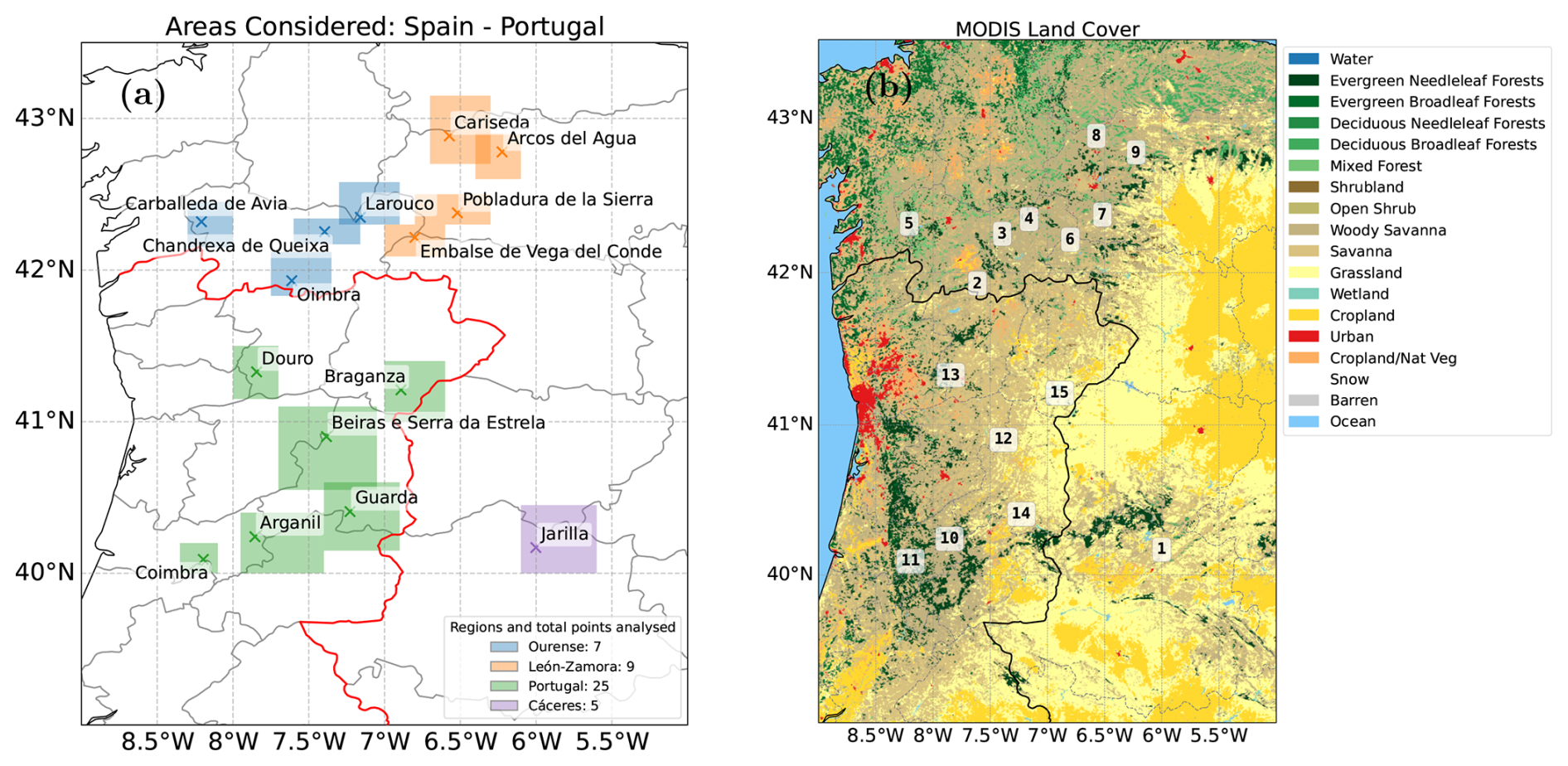
Figure 1 (a) Overview of the areas considered in this work with a total of 15 regions studied. Different regions are represented with different colours (b) MODIS Land Cover MCD12Q1 Version 6.1 data product with the International Geosphere–Biosphere Programme classification scheme.

2 Study area and fire events

The 2025 fire season was particularly severe in Spain and Portugal. According to the European Forest Fire Information System (EFFIS; Sedano et al., 2026), Spain recorded its most severe fire season since 2006 with a total of almost 0.4 Mha of burned area (nearly five times the 2006–2024 average), 83 % of which occurred in the month of August. Although Portugal suffered its worst fire season in 2017, 2025 was the second worst season since 2006 with almost 0.3 Mha burned, 73 % of which occurred also in August.

According to the yearly report provided by EFFIS (Sedano et al., 2026), in the month of August 2025, 0.334 Mha burned in Spain and 0.219 Mha burned in Portugal. In this work, a total burned area accounting for 0.388 Mha is studied, combining fires in Portugal and in Spain during August 2025. Thus, this study covers 70 % of the total area burned in the Iberian Peninsula during that month. In particular, we investigated the wildfires that occurred in August 2025 in 15 different regions in the Iberian Peninsula. Those wildfire regions or hotspots were named based on the different provinces or locations affected. Overall, a total of 46 TROPOMI overpasses were obtained for those 15 wildfire regions (i.e., most of the fires were observed during different days).

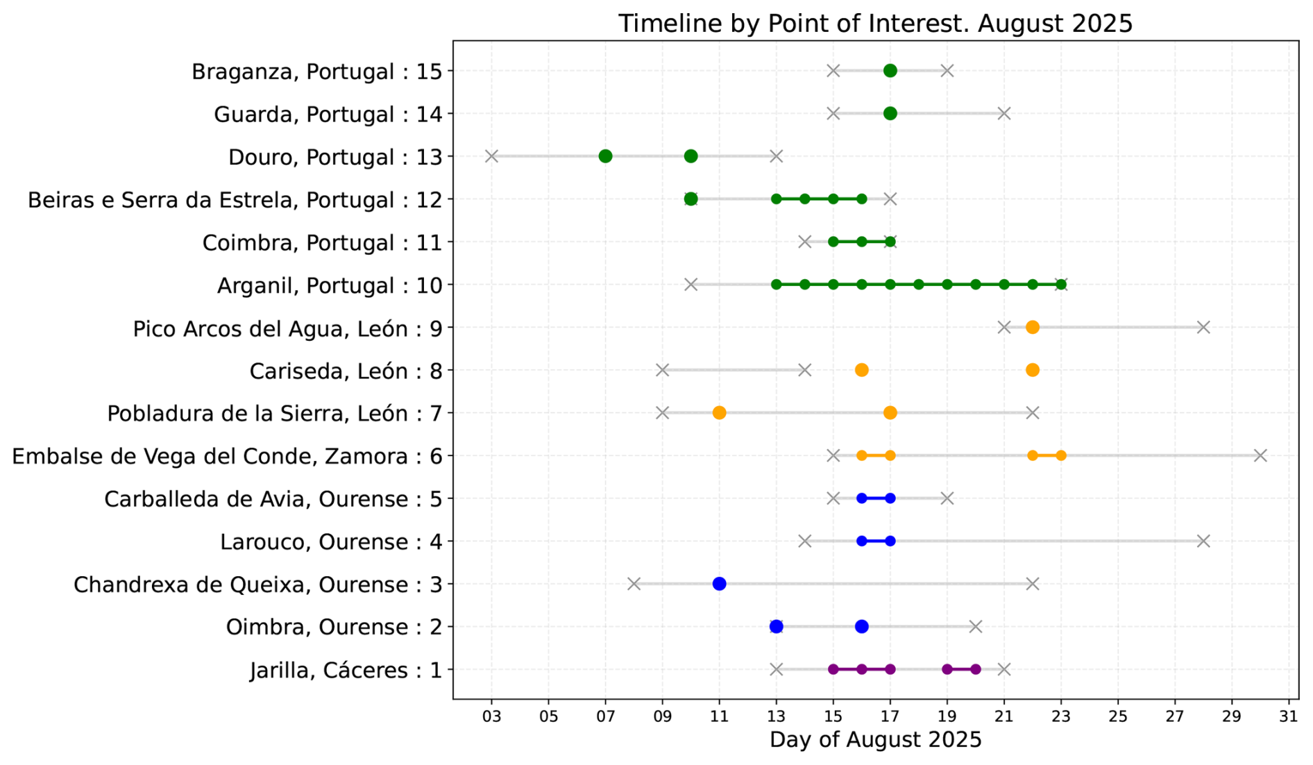
Figure 2 Timeline of the wildfires investigated during the month of August 2025, including the IDs of the regions of interest (Table 1). Colored points correspond to data in this work, following the same color scheme used in Fig. 1 for different regions. Gray lines and crosses correspond to the approximated initial and final day of the specific wildfire reported by supervised Sentinel-2 and MODIS from EFFIS. Note that, in case the wildfire was overpassed twice a day, only one single colored point is included.

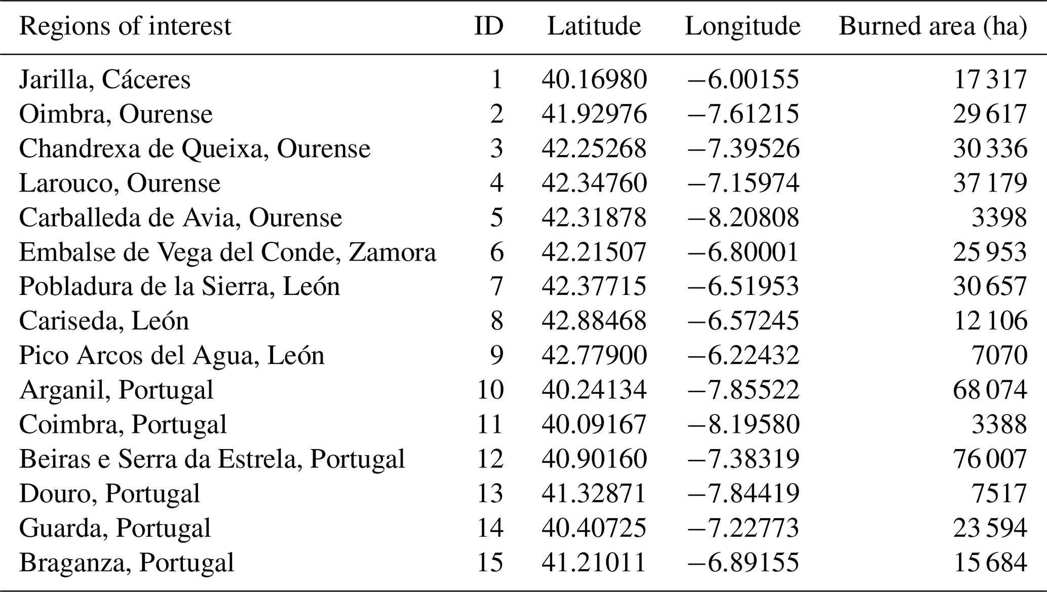
According to EFFIS, different types of biomes were burned within this August 2025. The distribution of biomass burned in Spain was: croplands 18 %, other natural lands 49 %, broadleaf forest 9.8 %, sclerophyllous vegetation 8.1 %, transitional 7.6 %. In Portugal: croplands 20 %, other natural lands 33 %, coniferous forest 6.4 %, transitional 35 %. Figure 1 shows the areas covered in this work, including the 15 specific wildfire regions studied. It also includes the land cover types according to the International Geosphere–Biosphere Programme (Seitzinger et al., 2015). A summary of the hotspot locations and the area burned for each site is shown in Table 1. Along this work, the different wildfire regions or hotspots will be referred to following the ID numbers provided in this Table 1.

The timelines of the different fires investigated in this work are provided in Fig. 2. These dates are obtained from Sentinel-2 and MODIS offered by EFFIS as supervised data. It should be noted, however, that these dates should be only regarded as indicative of start and end dates of active fires (EFFIS, 2020). Also, in case the wildfire was overpassed twice a day, only one single colored point is marked in Fig. 2.

Table 1 Regions of interest, IDs, hotspot latitude and longitudes and burned areas of the different fires studied in this work. Burned areas correspond to those reported by EFFIS.

3 Data

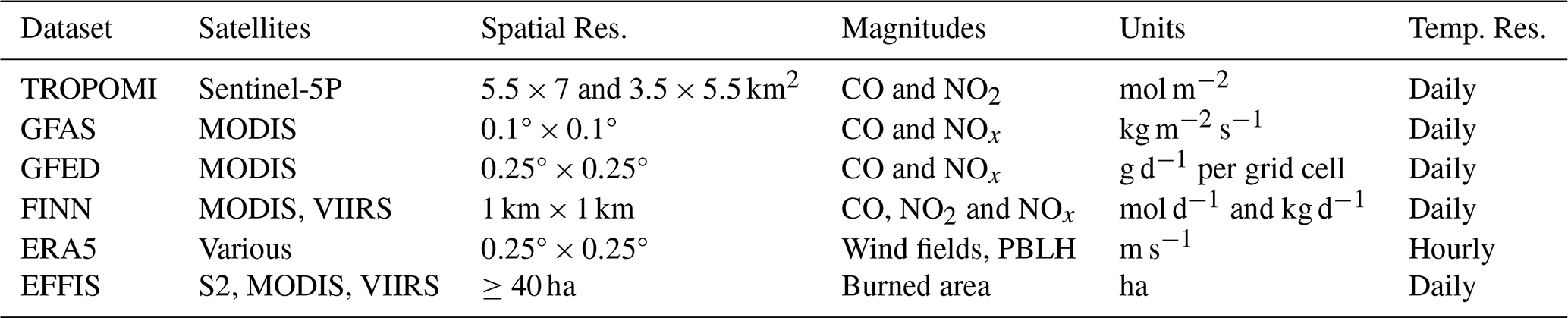
This work mainly builds on observations performed by the Tropospheric Monitoring Instrument (TROPOMI) above the Iberian Peninsula during August 2025. These measurements, along with ancillary data detailed below, are used to detect fire plumes and to infer top-down CO emission rates as detailed in Sect. 4.1. The satellite-based CO emission rates are then compared with emission estimates from different fire emission inventories. Moreover, the NO_x $/$ CO mole density ratio (MDR) derived from satellite and from inventories are also evaluated as a proxy for combustion efficiency (i.e., flaming vs smoldering combustion), type of biomass burning and EFs over fire lifecycles (Urbanski, 2013; van der Velde et al., 2021; Anderson et al., 2023). Table 2 shows a summary of the datasets used for our study.

3.1 TROPOMI observations

TROPOMI orbits the Earth in a Sun-synchronous orbit on board the Copernicus Sentinel-5 Precursor satellite, with a local overpass time of approximately 13:30. TROPOMI observations cover the solar spectrum in the ultraviolet-visible (UV-Vis, 270–500 nm), near-infrared (710–770 nm) and the short-wave infrared (SWIR, 2314–2382 nm). In this work, we focus mainly on the SWIR channel for CO observations, with a nadir spatial resolution of 5.5×7 km². In addition, NO₂ TROPOMI observations from the UV-Vis spectral range, with a nadir spatial resolution of 3.5×5.5 km², are also used in this work to assist with the fire plume masking (Sect. 4.1.2), and to investigate the NO_x $/$ CO MDR. While NO_x direct emission from fires is dominated by NO, the NO : NO₂ partitioning evolves very fast through oxidation and depends also on plume age and meteorological conditions (Andreae and Merlet, 2001; Griffin et al., 2021). Therefore, downwind satellite observations of NO₂ are often used to infer NO_x emissions (Beirle et al., 2021; Griffin et al., 2021). The methodology used to infer NO_x from NO₂ observations is further described in Sect. 4.3.

Details on the retrieval schemes used for CO and for NO₂ L2-level products are provided by Landgraf et al. (2016) and van Geffen et al. (2022), respectively. The quality of both products has been assessed in several comparison studies such as van Geffen et al. (2020, 2022) for NO₂ using the OMI instrument, and in Sha et al. (2021) using ground-based TCCON measurements. Particularly, TROPOMI observations in wildfire scenarios have been addressed before for NO₂ (Griffin et al., 2021; Wang et al., 2026), and for CO (Magro et al., 2021; Griffin et al., 2024; Voshtani et al., 2025; de Laat et al., 2026).

In this work, we use the off-line (OFFL) L2 TROPOMI products of CO and NO₂, obtained from the Copernicus Data Space Ecosystem website. Following previous TROPOMI-based fire studies, fire plumes can be labelled as clouds with standard quality filters. The quality assurance flag (“qa value”) used herein is set to higher than 0.5 in order to increase the number of pixels used close to fire hotspots, while still removing low quality data (Adams et al., 2019; Griffin et al., 2021, 2024; Wan et al., 2023). Note that applying the more standard and restrictive qa >0.75 threshold would have reduced the analysis to only 6 of the 46 investigated fire cases (13 %). Note also that the plume pixels retained in our analysis had mean qa values ≥0.7, consistent with plume pixels qa values obtained by Griffin et a. (2024). Relaxing the further this quality filter to qa >0 produced no systematic change in the retrieved quantities (Sect. S1.3 in the Supplement). The retrieval details used for the estimates reported in this work, including qa statistics for each fire case, are provided as Supplement.

3.2 Fire emission inventories: GFAS, GFED and FINN

3.2.1 Global Fire Assimilation System (GFAS)

We use the 1.2 version of GFAS assembled by the European Centre for Medium-Range Weather Forecast (ECMWF) within the Copernicus Atmosphere Monitoring Service (Kaiser et al., 2012). This dataset assimilates fire radiative power (FRP) from MODIS thermal infrared instruments on board the satellites Terra (overpasses at 10:30 and 22:30 local time) and Aqua (13:30 and 01:30; Remy and Kaiser, 2014). Considering these two satellites and different overpasses, GFAS offers daily estimates (0–23 h) of biomass burning emissions as fluxes (kg m⁻² s⁻¹) of several species such CO and NO_x, with a spatial resolution of 0.1°×0.1° (Wooster et al., 2005). To the authors' knowledge, no quantitative uncertainty estimates are reported for the GFAS emissions.

3.2.2 Global Fire Emissions Database (GFED)

Version 5.1 of GFED by NASA (van der Werf et al., 2025) is also used in this study. This dataset is based on the bottom-up approach estimating emission rates for several products by combining burned areas, fuel loads and combustion factors. EFs are based on biogeochemical modelling framework. This inventory offers monthly emission rates with a spatial resolution of 0.25°×0.25°. In addition, daily fluxes per grid cell (g d⁻¹) are also provided by combining monthly estimates with actives fires or burned area MODIS (or VIIRS) observations during that month. These daily emissions are the ones used herein. Although GFED uncertainties are difficult to assess, GFED documentation reports on 50 % uncertainty over large regions, depending on the burned area (van der Werf et al., 2025).

3.2.3 Fire Inventory from NCAR (FINN)

We also use emission estimates of the 2.5 version of FINN (Wiedinmyer et al., 2023). Similarly to GFED, this dataset is based on the bottom-up methodology (Wiedinmyer et al., 2011). This inventory is also based on MODIS and VIIRS fire observations and provides daily emission estimates by combining the area burned, the type of biomass and an EF. This dataset offers different product types. Herein we used the near-real time (NRT) with a spatial resolution of 1 km × 1 km. The uncertainties of FINNv2.5 remain unknown, although for FINNv1 they were estimated to be a factor of 2 (Wiedinmyer et al., 2011).

3.3 Ancillary data

In addition to TROPOMI observations and emission estimates from inventories, data from auxiliary sources was also used to characterize the meteorological conditions and fire events.

3.3.1 European Centre for medium-Range Weather Forecast Reanalysis (ECMWF)

The meteorological context of the wildfires is based on ERA-5, the 5th generation of ECMWF atmospheric reanalysis (Hersbach et al., 2020). This dataset provides several meteorological fields from 1940 to present, with an hourly temporal frequency on 0.25° horizontal resolution and 37 vertical pressure levels from 1000 to 1 hPa. The uncertainties for each variable are provided with 3 h frequency. In this work, the wind fields are used to compute TROPOMI-derived emission rates (Sect. 4.1).

3.3.2 European Forest Fire Information System (EFFIS)

EFFIS provides information on physical characteristics, evolution and statistics of wildfires in Europe (Camia et al., 2014; Vilar et al., 2015). Combining MODIS, VIIRS and Sentinel-2 observations, EFFIS maps represent about 95 % of the total burned area in the European Union every year and the service offers information on the burned area for Europe in the Rapid Damage Assessment (RDA) module. It has a daily frequency and it informs on fires of at least 30 ha burned, although smaller wildfires can be detected. The version 2.0 of the Current Situation Viewer produces active hotspots and burned area in a web portal (https://forest-fire.emergency.copernicus.eu/apps/effis.csv/, last access: 8 May 2026).

In this work, EFFIS is used to gather information on the area burned by a fire and the location of the sources. In the case of long-lasting and severe wildfires, the total burned area can be of hundreds of km². This is the case, for instance, of some of the fires investigated in this work, with total burned areas of more than 600 km² (60 000 ha) in some cases (Table 1). In these wide-spread cases, we chose the location of the source of the fire in the region (middle point) of the initial hotspot. Although EFFIS offers information on the start and final date of a fire, these dates are used herein only as a guidance since the exact time span of a given wildfire might differ from the exact dates of the emissions period investigated in this study. This is the case for the wildfire ID #8 in Fig. 2.

Table 2 Summary of the datasets used in this study, including sensor sources, spatio-temporal resolutions, quantities extracted and physical units.

4 Methods

4.1 Satellite-derived CO emissions rates

In order to retrieve CO emission rates from satellite observations of CO columns, we need to isolate the fire plumes from the background and calculate the respective CO enhancements. Thus, the first step is to calculate those background levels and subtract them from the signal. Then a plume masking algorithm selects the specific pixels associated to a plume of a given hotspot and, finally, we apply the Integrated Mass Enhancement (IME) method to infer emission rates.

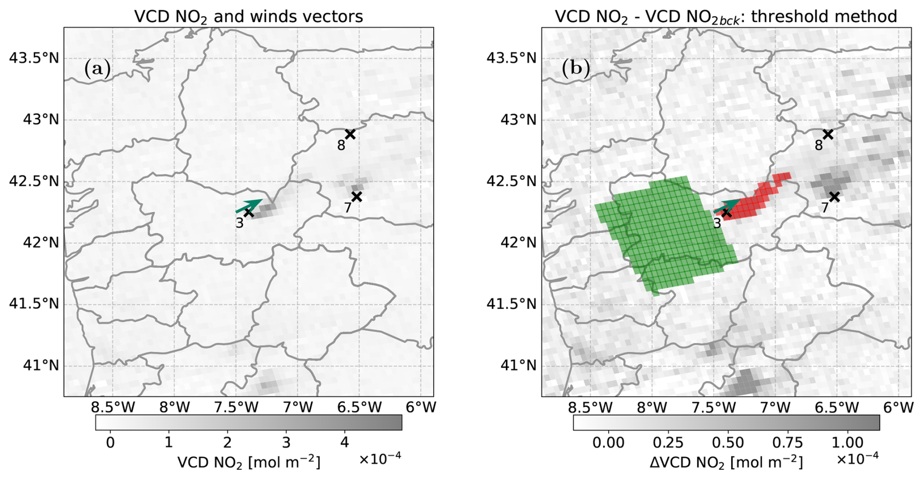
Figure 3 Representative complex scenario with neighbouring fires for a TROPOMI NO₂ overpass for point of interest #3 on 11 August 2025. Crosses and their numbers represent different points of interest (Table 1). The green arrow represents the nearest ERA5 point and the wind field direction. (a) L2 TROPOMI NO₂ (grey scale) raw overpass. (b) TROPOMI NO₂ background corrected and standard threshold plume masking method applied. Green pixels correspond to the upwind area selected as background whereas red pixels are the standard threshold plume masking.

4.1.1 Background subtraction

Many background subtraction methods have been employed in the literature in the context of TROPOMI trace gases, such as a percentile approach taking a fixed region (Plant et al., 2022) or a specific background model (Tu et al., 2022). Here we use an upwind method. It is based on taking the background in a fixed region in the upwind direction from the source. This approach has been used previously for TROPOMI-related studies (Lama et al., 2020), including in a wildfire context (Griffin et al., 2021, 2024). Herein, the background region is taken as a 0.8°×0.6° square shape (orthogonal × parallel to the wind direction, Fig. 3), similar to the work of Griffin et al. (2021, 2024). Therefore, the TROPOMI overpass is corrected from its background as follows:

$$\begin{array}{}\text{(1)}& \mathrm{\Delta }{\mathrm{VCD}}_i={\mathrm{VCD}}_i-{\mathrm{VCD}}_{\mathrm{back}},\end{array}$$

where VCD_i is the vertical column density for pixel i, ΔVCD_i the column enhancement and VCD_back corresponds to the background value, both in units of mol m⁻². The background value is computed as the mean within the background region defined above.

Note that with this upwind background method, we specifically capture the composition of the air parcel before it reaches the target fire. Additionally, this method will incorporate in the background subtraction possible contributions of upwind fires. The sensitivity of the results to the choice and size of the background region is assessed in Sect. S1.4.

4.1.2 Plume masking

Once the background is subtracted, a plume masking algorithm is deployed with the aim of selecting the plume associated to individual fire events. Previous studies have used a standard threshold method for plume masking, in which plume pixels are identified as those representing an anomaly with respect to a specific background (Finch et al., 2022; Lauvaux et al., 2022; Schuit et al., 2023). In this standard approach, a pixel is classified as part of a plume when its background-corrected column exceeds a threshold defined from the mean and standard deviation of the background field. Further details of this threshold method are provided in Sect. S2.1.

In this work, we develop a novel “synergy” method, which facilitates the distinction between plumes of neighbouring fires and provides results compatible with established standard threshold methods for simple plume cases (Sect. S2.2). This synergy method is based on the idea of using NO₂ fields to constrain the CO plume masking in complex multi-fire scenes, exploiting collocated and simultaneous NO₂ and CO satellite observations above the same region. This method relies on the shorter lifetime of NO₂ compared to CO (hours versus months; Novelli et al., 1998; Beirle et al., 2011; Adams et al., 2019; Wan et al., 2023). Thus, compared to CO, NO₂ plumes are generally narrower, more compact and found closer to fresh fire plumes (Griffin et al., 2021).

For the synergy plume masking method, we first isolate the NO₂ plume according to a standard threshold plume masking approach (Sect. S2.1 and Eq. S3). In that case, the threshold parameter defining the required enhancement above background variability, is typically selected between 3.5 and 5.5, depending on plume complexity. Figure 3 shows an example of the performance of the standard threshold method for NO₂ fields for a scene with multiple fire hotspots.

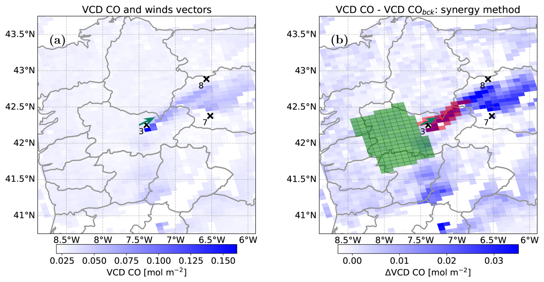
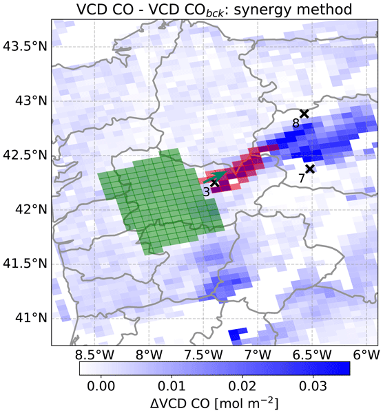
Figure 4 Representative complex scenario with neighbouring fires for a TROPOMI CO overpass for wildfire ID #3 on 11 August 2025. Crosses and their numbers represent different hotspots (Table 1). The green arrow represents the nearest ERA5 point and the wind field direction. (a) L2 TROPOMI CO (blue scale) raw overpass. (b) TROPOMI CO fields, background corrected and synergy plume masking method applied. Green pixels correspond to the upwind area selected as background whereas red pixels are the standard threshold plume masking.

Once a plume area has been defined based on NO₂ fields, we extract the location information of the centre of those plume pixels and transfer them into the CO fields (i.e. every CO pixel containing that location is considered as “plume”). Only those plume pixels will be further used for retrieving CO emission rates. An example of this idea is schematized in Fig. 4 for CO fields, where the NO₂ plume area shown in red in Fig. 3, is applied to the CO fields.

4.1.3 Integrated Mass Enhancement (IME)

We use the Integrated Mass Enhancement method (IME; Varon et al., 2018) to estimate the CO emission rates from satellite measurements. This method has been extensively applied previously for different trace gases (Griffin et al., 2021; Maasakkers et al., 2022; Schuit et al., 2023; Santaren et al., 2025; Zhang et al., 2025) and applied also in other studies concerning CO emissions from wildfires (Griffin et al., 2024). For long-lived species, the IME method calculates emission rates E via

$$\begin{array}{}\text{(2)}& E={\displaystyle \frac{u\cdot M_{\mathrm{m},\mathrm{CO}}}{L}}\sum _i^n\mathrm{\Delta }{\mathrm{VCD}}_i\cdot A_i,\end{array}$$

where u is the wind speed in m s⁻¹, M_m,CO= 28.01 g mol⁻¹ is the CO molar mass, ΔVCD_i is the vertical column density enhancement in mol m⁻² for each plume pixel i following the procedure explained in Sect. 4.1.1 and 4.1.2., A_i is the pixel area in m² and L is the plume length in m. In this work, $L=\sqrt{{\sum }_i{A}_i}$, i.e. the square root of the plume area (Maasakkers et al., 2022; Zhang et al., 2025). This quantity is an approximation of a characteristic plume length, other magnitudes can be chosen as suggested in Varon et al., (2018). The sum of the previous equation runs over $i=\mathrm{1},\mathrm{\dots },n$ where n is the number of the plume pixels. Equation (2) retrieves the emission rate E of a source in units of g s⁻¹. As mentioned before, throughout this work we present emission rates in t h⁻¹. In this work, the wind speed u is computed using ERA5 data on pressure levels (Sect. 3.3.1), considering wind profiles within ±2 h of the time of the TROPOMI overpass to account for temporal variability. Wind speed is averaged in time and altitude within the planetary boundary layer (PBLH, provided by ERA5; Fioletov et al., 2015) and its standard deviation is considered for uncertainty estimation. The wind direction used for the plume masking is calculated by computing the angle between u and v averaged components of the wind fields. The error and uncertainties of our IME method are addressed in Sect. S1.1.

4.2 Inventories emission rates

In this work, emission rates are also obtained from the fire emission inventories GFAS, GFED and FINN, detailed in Sect. 3.2. The pipeline followed by the three inventories is similar regardless of the trace gas addressed. However, two differences should be taken into consideration. On one hand, GFAS and GFED report emissions aggregated over regular latitude–longitude grid cells of fixed spatial resolution, while FINN provides emissions as individual hotspot points. On the other hand, GFAS provides emission rate densities in units of kg s⁻¹ m⁻², whereas GFED gives emission rates in units of g d⁻¹ per grid cell and FINN in units of kg d⁻¹ per km² for CO and NO₂ and mol d⁻¹ for reactive nitrogen NO_x.

In this work, the emission rates from inventories are computed by taking a fixed area around the hotspot, obtained from EFFIS (see Sect. 3.3.2) and listed in Table 1. All the points within this area are summed up to compute the total emission rates. Since GFAS provides emissions per area, the area of each pixel is taken into account as follows

$$\begin{array}{}\text{(3)}& E=\sum _j^m{A}_j{\mathit{\rho }}_j,\end{array}$$

where A_j is the area of each pixel in units of m² and ρ_j is the surface emission rate of the pixel j. Index runs over $j=\mathrm{1},\mathrm{\dots },m$ with m the number of pixels enclosed within the given area.

The formulation for FINN and GFED is slightly different, described as

$$\begin{array}{}\text{(4)}& E=\stackrel{m}{\sum _j}{e}_j,\end{array}$$

where e_j is the emission rate for the pixel j. Similarly, index runs over $j=\mathrm{1},\mathrm{\dots },m$ with m the number of pixels or independent hotspots enclosed within the given area, for GFED and FINN, respectively. Herein all emission rate units are transferred to t h⁻¹.

Regarding uncertainties, although the three inventories suggest that they are still unknown, van der Werf et al. (2025) stated that GFED uncertainties could be at least 50 %, whereas Wiedinmyer et al. (2023) suggested that FINNv1 uncertainties could reach a factor of 2. In this work, we consider an overall 50 % uncertainty in all inventory data.

4.3 NO_x $/$ CO Mole Density Ratio (MDR)

In addition to comparing top-down and inventory-based CO emission rates, we also analyse the relative abundance of reactive nitrogen and CO in the fire plumes using NO_x $/$ CO MDR from satellite observations and from inventories.

Regarding satellite observations, although TROPOMI does not measure NO_x directly, part of the NO emitted by the fire is converted to NO₂ during plume transport. Therefore, the NO₂ observed by the satellite downwind of the source includes directly emitted NO₂ and also NO₂ produced chemically from emitted NO. Previous satellite-based studies have inferred a NO₂-to-NO_x conversion factor to relate the observed NO₂ signal to total NO_x (Beirle et al., 2021; Griffin et al., 2021). For biomass-burning plumes, Griffin et al. (2021) found that net NO_x emissions are approximately 1.3–1.5 times larger than NO₂ emissions derived from satellite down-wind observations. Beirle et al. (2021) reported a comparable conversion for NO_x point sources. In this work, the TROPOMI NO₂ $/$ CO MDR is defined as

$$\begin{array}{}\text{(5)}& \mathrm{MDR}={\displaystyle \frac{{\stackrel{\mathrm{‾}}{\mathrm{\Delta }\mathrm{VCD}}}_{{\mathrm{NO}}_{\mathrm{2}}}}{{\stackrel{\mathrm{‾}}{\mathrm{\Delta }\mathrm{VCD}}}_{\mathrm{CO}}}}\times {\mathrm{10}}^{\mathrm{3}},\end{array}$$

where ΔVCD is the average value for all plume pixels in units of mol m⁻². The factor 10³ ensures that MDR is in units of mmol mol⁻¹. MDR uncertainties are assessed in Eq. (S2) in the Supplement. This MDR is then scaled by a factor of 1.3–1.5 to obtain an approximate satellite-based NO_x $/$ CO MDR to compare with inventories.

For the case of MDR inferred from inventories, we use the following formulation:

$$\begin{array}{}\text{(6)}& \mathrm{MDR}={\displaystyle \frac{E_{{\mathrm{NO}}_x}}{E_{\mathrm{CO}}}}{\displaystyle \frac{M_{\mathrm{m},\mathrm{CO}}}{M_{\mathrm{m},{\mathrm{NO}}_x}}}\times {\mathrm{10}}^{\mathrm{3}},\end{array}$$

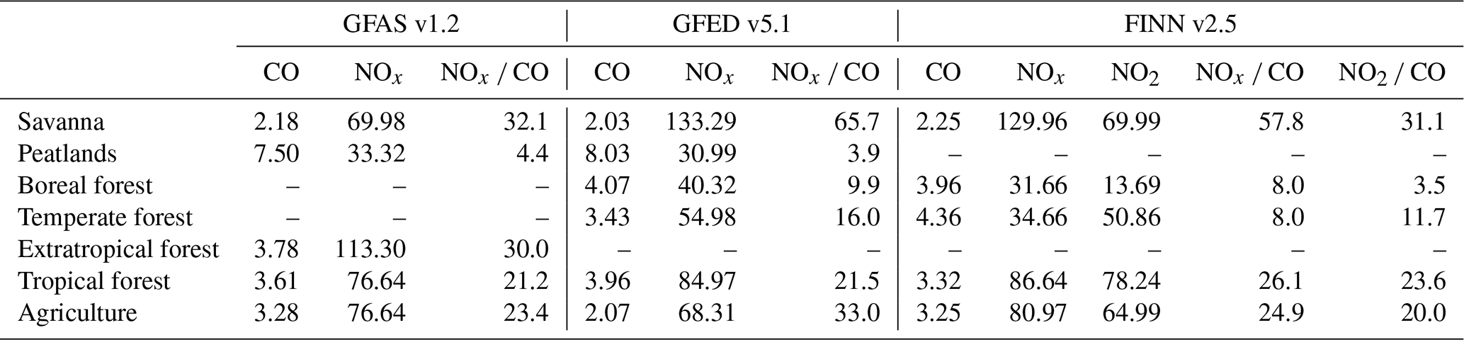
where E_gas is the inventory emission rates in t h⁻¹ defined in Eqs. (3) and (4). The factor M_m,gas is the molar mass of the specific gas, where the values of $M_{\mathrm{m},\mathrm{NO}}=\mathrm{30.01}$ and $M_{\mathrm{m},\mathrm{CO}}=\mathrm{28.01}$ g mol⁻¹ have been used. The molar mass of M_m,NO is used to compute NO_x values, since all the inventories retrieve NO_x as NO (Andreae and Merlet, 2001; Wiedinmyer et al., 2023; van der Werf et al., 2025). The factor 10³ ensures that MDR is in units of mmol mol⁻¹. Exchanging NO_x by NO₂, with $M_{\mathrm{m},{\mathrm{NO}}_{\mathrm{2}}}=\mathrm{46.01}$ g mol⁻¹, this equation applies also for MDR NO₂ $/$ CO calculation in the case of FINN, since this inventory provides not only NO_x but also NO₂. The inventory MDRs depend on the EF associated to a type of biomass burned. Table 3 provides a summary of the EFs of NO_x and CO for different type of vegetation as provided by each inventory. Additionally, as linked to NO_x $/$ CO, the NO_x $/$ CO EF ratios of each inventory and fuel type are also shown.

Table 3 Summary of EFs and vegetation type provided by each inventory used in this work (in mol units). CO is expressed in mol, while NO_x and NO₂ are expressed in mmol. Ratios are expressed in mmol mol⁻¹.

5 Results and discussions

5.1 Assessment of CO emission estimates

5.1.1 Satellite-based CO emission rates

All CO emission rates provided in this work were computed using the synergy plume masking method. While emission estimates from the standard threshold method and the synergy method agree for simple scenes (see Supplement Fig. S7), the synergy method allowed us to infer emissions rates from complex scenarios with multiple fires burning simultaneously in the vicinity. An example of the main advantage of using this synergy method for differentiating individual plumes in such complex situations is shown in Fig. 5 for the 16 August (another example can be found in Fig. S16). Note that in this scene, up to 6 fires are active at the same time (#2, #3, #4, #6, #7 and #8) and, eventually, the direction of the wind contributes to the mixing of the different CO plumes. On this scene, the standard threshold plume masking method is not able to detect separate plumes (Fig. 5a), resulting in a masked plume containing CO contribution from 6 different active hotspots. Note that the standard threshold plume masking in Fig. 5a is applied over #4 but one would find a similar plume masking regardless the point of interest.

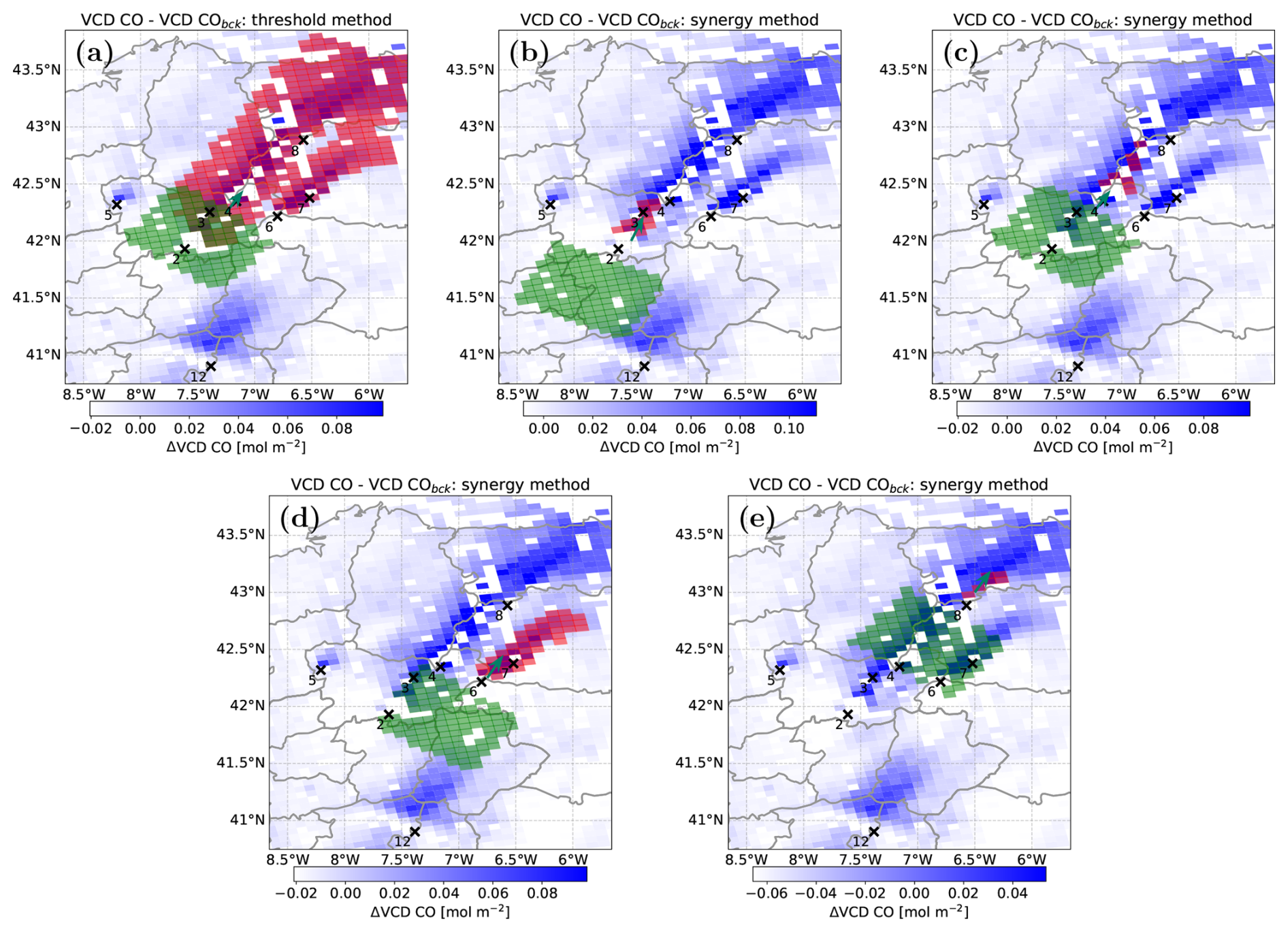
Figure 5 Representative CO TROPOMI background corrected overpasses on 16 August 2025. (a) CO standard threshold plume masking method applied at wildfire ID #3. The rest of the panels correspond to synergy plume masking applied at the wildfire IDs (b) #2. (c) #3. (d) #8. (e) #6.

To quantify the benefit of the synergy method, we investigate the inferred emission rates. According to Eq. (2), the emission estimation is directly proportional to the wind speed. The synergy method allows us to assign a specific wind speed to each specific hotspot. Since in complex scenarios, hotspots could be separated from each other by hundreds of kilometres, the wind field could vary significantly between different hotspots. We can quantify this distinction by comparing the resulting emissions when using the standard threshold method and comparing it to the synergy method.

Figure 5a estimates a CO emission rate for hotspot #3 of 1417 t h⁻¹ by using the standard threshold plume masking with a wind speed of 4.2 m s⁻¹ for the entire scene. However, as can be seen in that figure, that #3 hotspot's plume delimited by the standard threshold method spans above several other hotspots burning simultaneously (#4, #6, #7, #8). In the other panels in Fig. 5, we applied the synergy method for the individual fire events and estimate (b) hotspot #2, emitting 552 tCO h⁻¹ with 3.6 m s⁻¹, (c) hotspot #3 emitting 868 tCO h⁻¹ with 4.2 m s⁻¹, (d) hotspot #8 emitting 231 tCO h⁻¹ with 4.0 m s⁻¹ and (e) hotspot #6, emitting 1207 tCO h⁻¹ and 5.9 m s⁻¹. Therefore, if only the standard threshold plume masking were considered for hotspot #3, the inferred emission rate would be biased, influenced by the other fires. This difference could originate from the difference in the wind speed, for instance, between panels (a) and (e) differing by nearly 50 %.

Although indeed the synergy approach allows us to isolate some sources in very complex situations, in extreme cases when hotspots are too close and wind conditions are not favourable, this method cannot distinguish individual fires either. For instance, in Fig. 5c and e, respectively, hotspots #3, #4 and #6, #7 cannot be disentangled. In such complex situations, we consider both hotspots as one source for TROPOMI and the inventories. Nevertheless, given the variability of fire and wind scenarios investigated in this work, in the following the reported emission rates and MDR inferred from TROPOMI are based on the synergy plume masking method.

Since the IME approach (Sect. 4.1.3) used in this work relates plume enhancements to wind speed (Eq. 2), the retrieved emission rates are expected to be sensitive to the chosen wind field. In fact, this variable introduces one of the largest uncertainties for the emissions rates retrieved, accounting for approximately 80 % of the estimated uncertainty as further discussed in the Supplement. We additionally assessed the sensitivity to the vertical layer used to represent plume transport by varying the altitude range over which ERA5 winds were averaged (Sect. S1.5). The resulting emission estimates showed only limited systematic sensitivity to this choice, although extending the averaging layer above the PBL increased the wind variability and, consequently, the uncertainty for some individual cases. Note, however, that the 0.25° ERA5 spatial resolution may not fully resolve local wind variability associated with the complex terrain of the study region.

The sensitivity of our results to background selection was also investigated (Sect. S1.4). Changing the size of the upwind background region produced little systematic effect on the retrieved CO emission rates, whereas the use of a fixed pre-fire regional background resulted in systematically higher estimates (∼39 %). The latter reflects the elevated regional CO background during the multi-fire episode and supports the use of a scene-specific upwind background for the conditions investigated herein.

The CO emission rates we infer from TROPOMI observations reveal a large event-to-event variability as shown in Fig. 6. Overall, we estimate emission rates for 46 hotspots in the month of August 2025 in the northwestern region of the Iberian Peninsula. Most (93.5 %) of those fires emitted less than 2000 tCO h⁻¹ each. The highest emission rates were observed on 15 August 2025 for two of the largest Portuguese wildfires of the last decade: Arganil (#10), emitting over 3000 t h⁻¹, and Beiras e Serra de Estrela (#12), with 5500 t h⁻¹ emitted.

In addition to the uncertainties discussed above, other sources of error may affect our satellite-based estimates. Misalignments between the CO and NO₂ TROPOMI ground pixels and possible differences in the lifetime and vertical distribution of both species, may also affect the plume definition when NO₂ is used to constrain our CO fields. Furthermore, an additional source of uncertainty arises from the different sensitivity of the TROPOMI NO₂ and CO retrievals to scattering linked to fire-related aerosols (Griffin et al., 2021). Under fire conditions, NO₂ retrievals may be affected by aerosol scattering and by the assumed NO₂ a priori vertical profile, particularly for enhancements close to the surface. These effects are expected to be smaller for TROPOMI CO VCDs because of its different spectral sensitivity to scattering. Since NO₂ is used in this work to constrain the plume mask and to derive the NO₂ $/$ CO MDRs, these NO₂ retrieval uncertainties may propagate into our CO emission and MDR estimates. Sensitivity tests indicate little systematic effect on the CO emission estimates for moderate (± 20 %) NO₂ perturbations, although individual retrievals and the MDRs can be more sensitive. These aspects are further discussed throughout Sects. S1 and S3.

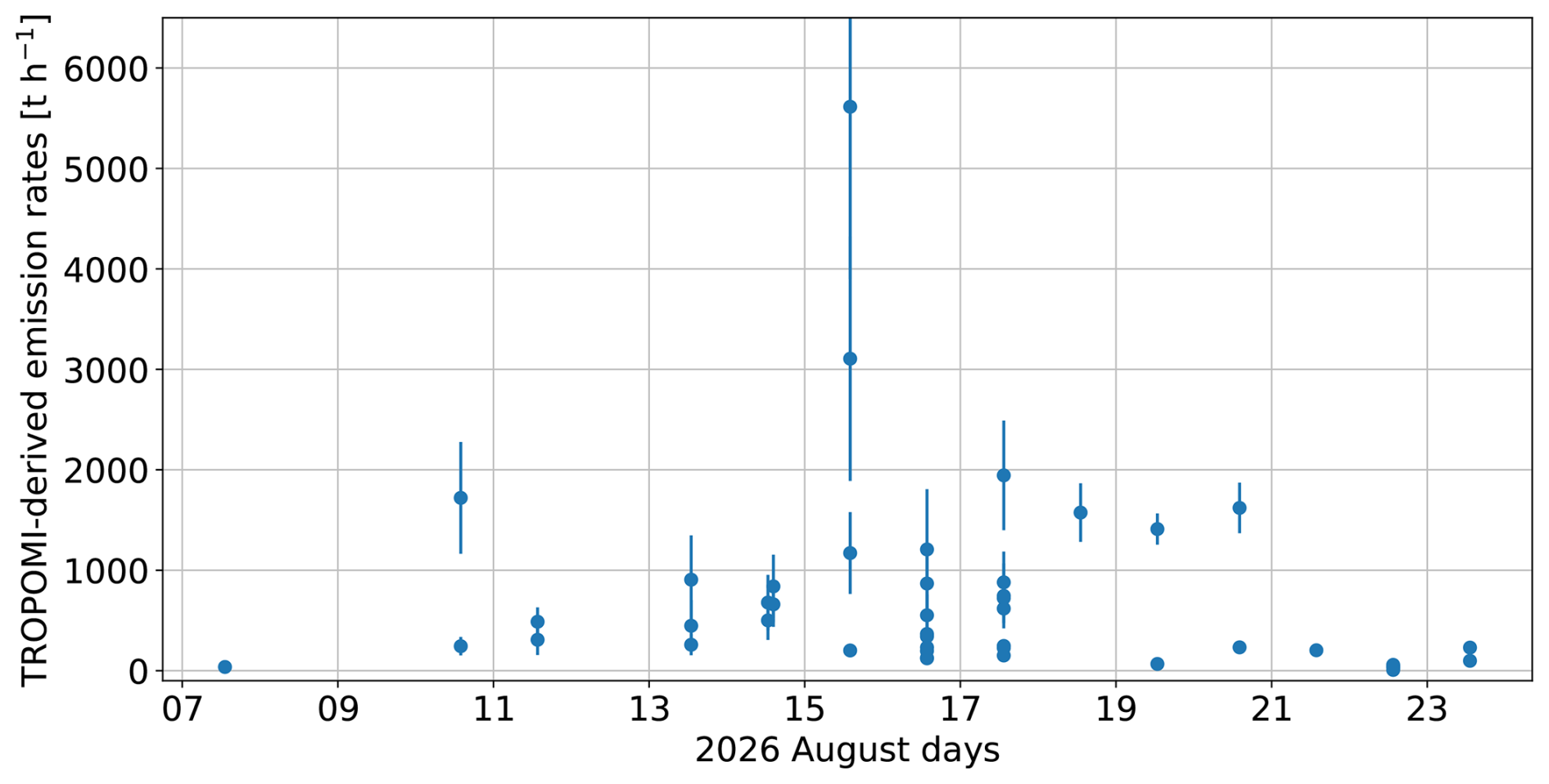
Figure 6 TROPOMI-derived CO emission rates (t h⁻¹) for the 46 hotspot overpasses retrieved during August 2025 in the northwestern Iberian Peninsula. Error bars represent the uncertainty in the emission rate estimates (Sect. S1).

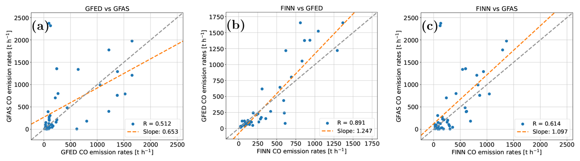
Figure 7 Inter-comparison of CO emission rates (t h⁻¹) between GFED, GFAS, and FINN inventories: (a) GFAS vs. GFED, (b) GFED vs. FINN, and (c) GFAS vs. FINN. The grey dashed line shows the 1:1 correspondence, and the orange dashed line represents the linear trend. Correlation coefficients (R) and slopes are shown in each panel.

5.1.2 Evaluation of the inventory emission estimates

Figure 7 shows the comparison of the CO emission rates inferred from the three inventories used in this work for the 46 individual spots investigated. Results indicate that the emission inventories agree on the magnitude of emissions. However, for individual plumes, there are substantial differences between inventories. GFED and FINN show the strongest consistency (R∼0.89), with a high and significant correlation, with GFED values 25 % larger than FINN's. In contrast, GFAS correlates worse with GFED and FINN.

For the wildfires studied in this work, the overall EFs derived from these inventories agree to within ±30 %–40 %. However, the rather low correlation values of some of the comparisons suggest limited event-to-event consistency (Fig. 7). In particular, the GFAS inventory shows the lowest correlation in this inter-comparison, finding R∼0.51 and 0.61 with GFED and FINN respectively. Moreover, two apparent GFAS outliers seem to appear for values larger than 2000 t h⁻¹, not found in either GFED or FINN estimates (panels (a) and (c) of Fig. 7 respectively).

Previous inventory intercomparison studies have shown that differences between fire emissions depend on region, fire type, temporal aggregation and inventory version (e.g., Faulstich et al., 2022; Yang et al., 2026). For instance, Wiedinmyer et al. (2023) reported a large difference of CO emission estimates by FINNv1.5 and FINNv2.5, with the estimates of FINNv2.5 being up to a factor of two higher than FINNv1.5. The study suggests similar factors between estimates from FINNv2.5 and GFEDv4 and GFASv1, with FINNv2.5 reporting higher values also depending on the region. Griffin et al. (2024) also showed that the level of agreement among inventories strongly depends on the region, with some regions showing agreement within about a factor of two and others showing much larger discrepancies. Similarly, the work of van der Werf et al. (2025) found that GFEDv5 CO emission estimates are a factor of approximately 1.5 higher than the previous GFED version.

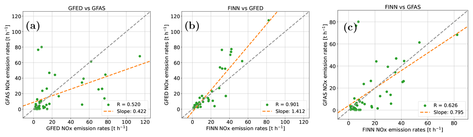
Figure 8 Inter-comparison of NO_x emission rates (t h⁻¹) between GFED, GFAS, and FINN inventories: (a) GFAS vs. GFED, (b) GFED vs. FINN, and (c) GFAS vs. FINN. The grey dashed line shows the 1:1 correspondence, and the orange dashed line represents the linear trend. Correlation coefficients (R) and slopes are shown in each panel.

Regarding NO_x emission estimates from inventories, the internal consistency from the inventories is investigated in Fig. 8. Similar to the CO assessment above, GFED and FINN show the strongest correlation for NO_x emissions, although FINN's values are approximately 30 % smaller than GFED's.

Overall, our inventory intercomparison is consistent with previous works showing that fire emission estimates can agree in bulk magnitude while still differing substantially for individual fires, with the different CO and NO_x EFs adopted by the inventories (Table 3) potentially contributing to these differences.

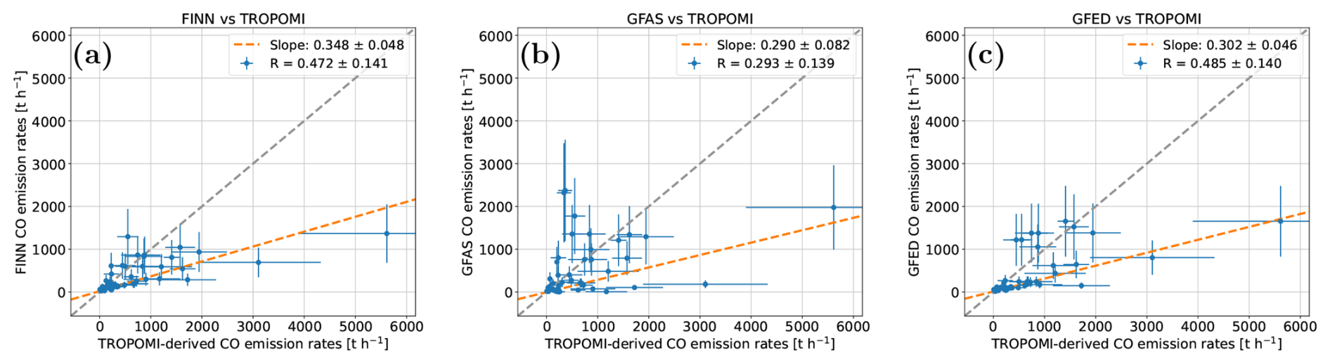
Figure 9 Comparison of emission rates (t h⁻¹) between inventories and TROPOMI-derived estimates: (a) FINN vs. TROPOMI-derived, (b) GFAS vs. TROPOMI-derived, and (c) GFED vs. TROPOMI-derived. Blue markers include horizontal (TROPOMI) and vertical (Inventories) error bars indicating estimate uncertainties. The grey dashed line shows the 1:1 correspondence, and the orange dashed line represents the linear trend. Correlation coefficients (R) and slopes are shown in each panel.

5.1.3 Comparison between TROPOMI and inventories CO emission estimates

The comparison of the CO emission rates inferred from the three inventories used in this work and from TROPOMI observations, is shown in Fig. 9. In general, correlations are weaker between observation-based estimates and inventories than between inventories. Similarly to Fig. 7, the GFAS inventory shows a poor correlation with TROPOMI finding R∼0.29 in panel (b), whereas FINN and GFED seem to show a slightly better correlation with R ∼0.48 in panels (a) and (c), respectively. In addition to these satellite-inventories moderate correlations, the results for the 46 fires investigated herein suggest a systematic low bias of the CO emissions inferred from inventories compared to those inferred from TROPOMI observations (Fig. 9). For the wildfires studied, the CO emissions inferred from TROPOMI observations are approximately 3 times higher than those retrieved from inventories (factor 2.9 for FINNv2.5, 3.4 for GFASv1.2 and 3.3 for GFEDv5.1), suggesting a significant underestimation of CO emissions by the inventories despite large scatter. This underestimation is robust against outliers. In particular, when removing the largest TROPOMI values of ∼3000 and 5500 t h⁻¹, the slopes remain unchanged, suggesting that the significant higher TROPOMI estimates are not driven by the large fire events only. Note that the different spatial resolution of the inventories compared to TROPOMI data (Table 2: GFED 0.25°×0.25°, GFAS 0.1°×0.1°, FINN 1 km × 1 km, TROPOMI 5.5 km × 7 km) is unlikely to be the reason behind the TROPOMI-inventory discrepancies found in Fig. 9. Despite their different spatial resolution, all inventories provide CO emission rates ∼ 3 times lower than our TROPOMI estimates. Also, the correlations found with TROPOMI data were ∼ 0.48 for FINN (with smallest spatial resolution) and GFED (with biggest resolution); very similar to the correlation e.g. GFED-GFAS (Fig. 7a). Further sensitivity tests on the possible effect of the different spatial resolution of inventories and of TROPOMI data are provided in Sect. S4.

Previous direct comparison of TROPOMI-derived CO emission rates and inventory ones is shown in the work of Griffin et al. (2024). In that work, based on 4000 TROPOMI observations above fires, the authors found that emission rates derived from TROPOMI were 4.8 times higher than those inferred from Global Forest Fire Emissions Prediction System (GFFEPS) inventory, with similar correlation as our study. Although GFFEPS is not one of the inventories used herein, Anderson et al. (2024) showed that global annual GFFEPS carbon emissions are of the same order as other commonly used fire emission inventories, corresponding to about 80 % of GFAS, 74 % of GFEDv4.1 and 97 % of FINNv1.5 over 2015 to 2020. Griffin et al. (2024) suggested that part of the difference between satellite and GFFEPS based emission estimates could be related to different temporal sampling and prescribed GFFEPS diurnal profile. Although their specific explanation referred to GFFEPS, the broader issue is also relevant to this work. The inventories used in our work only provide daily mean estimates. However, since the integrated plume mass observed by TROPOMI (Eq. 2) contains emissions released during transport prior to the overpass over a characteristic timescale of approximately $L/u$. Thus, our TROPOMI-derived emissions should be interpreted as overpass-centred, short-timescale emission estimates. If fire activity around the TROPOMI overpass (∼ 13:30) is not representative of the corresponding daily inventory estimate, this temporal mismatch may contribute to both the scatter and part of the systematic TROPOMI–inventory difference. However, the similar factor of 3 found independently for GFAS, GFED and FINN suggests that differences in the temporal sampling are unlikely to be the only explanation for the discrepancy shown in Fig. 9.

In addition to the direct comparison of TROPOMI overpasses with GFFEPS aforementioned, Griffin et al. (2024) also used fire energy-constrained TROPOMI observations to derive annual CO emissions and compared those estimates with several inventories (GFFEPS, GFAS, GFED, FINN v1.5 and FINN v2.5). Their results showed that the agreement was region-dependent. Although their comparison is not directly equivalent to the fire-by-fire overpass analysis performed herein, it supports the concept that differences between satellite and inventory estimates can arise from inventory-dependent assumptions and regional fire characteristics. TROPOMI-constrained CO emission in wildfires scenarios was also investigated by van der Velde et al. (2021) and Voshtani et al. (2025). For the 2023 Canadian wildfires, Voshtani et al. (2025) found that the CO observations were better reproduced after increasing the prior emissions by factors of 3.0, 2.6 and 1.4 for Quick Fire Emission Database (QFED), Global Biomass Burning Emission Product (GBBEP) and GFAS, respectively. In the case of 2019–2020 Australian fires, van der Velde et al. (2021) also obtained posterior CO emissions higher than the prior inventory estimates, suggesting a factor of 2–3 (depending on the month investigated). Overall, considering the large uncertainties linked to TROPOMI and inventory-based CO emission estimates reported herein, results for the 2025 Iberian wildfires are consistent with previous studies suggesting inventory underestimation during intense wildfires. However, given the event-to-event scatter and the uncertainties affecting both satellite and inventory estimates, the ×3 factor found in our work should not be interpreted as event-to-event factors. Note, however, that the similar offset obtained for all three inventories, together with the sensitivity analyses presented in the Supplement, indicates that the ×3 factor difference is robust to the methodological choices tested in this work. Our results therefore suggest a systematic low bias of the inventory estimates relative to the TROPOMI-derived CO emissions for the fires and sampling conditions considered in this study.

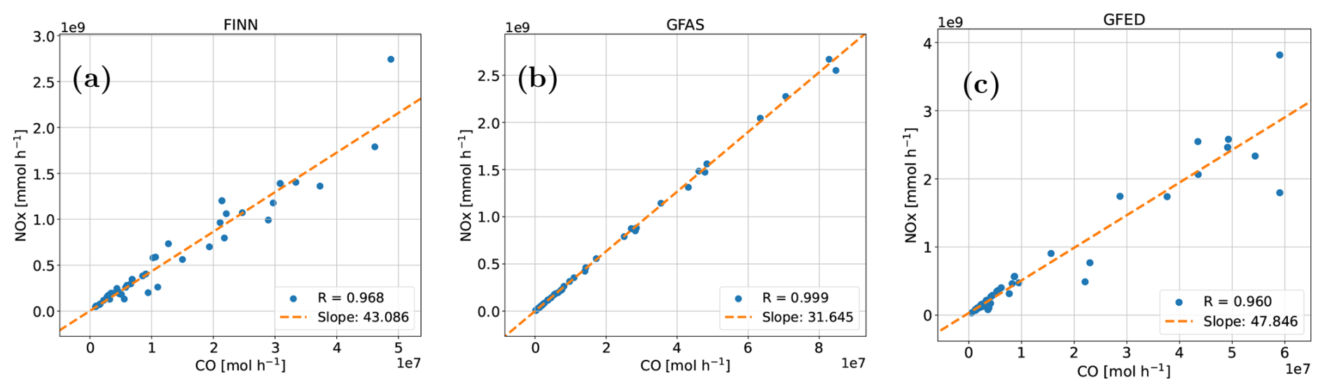
Figure 10 Intra-inventory correlation between NO_x and CO emission rates for (a) FINN, (b) GFAS, and (c) GFED. The dashed orange line represents the linear fit.

5.2 Evaluation of the NO_x $/$ CO MDR

5.2.1 Internal consistency between inventories

In order to assess the combustion efficiency and possible fuel type for our 46 case studies from the inventories perspective, following the work of van der Velde et al. (2021), we investigate the correlation between NO_x and CO emission rates inferred from each inventory. Results are shown in Fig. 10.

The three inventories show strong and significant NO_x to CO mole density correlations, indicating that both species scale coherently with fire strength within each inventory. However, since the NO_x $/$ CO MDR can be used as a proxy for combustion efficiency, the different slopes inferred for each inventory (Fig. 10) may indicate that the inventories assign different effective combustion characteristics to the same fire events.

The slopes found in Fig. 10 are in the upper range of the EF ratios shown in Table 3. For GFAS it is found that the slope matches with the ratio for savanna fires, while the GFED and FINN slopes are slightly lower than their EF ratios suggesting that combinations of different biomes, including agriculture and forest, need to be considered.

5.2.2 MDR derived from satellite

TROPOMI-based NO₂ $/$ CO MDR (Eq. 5) can provide valuable information regarding type of vegetation burned in a fire (van der Velde et al., 2021). Herein, we investigate the satellite-based NO₂ $/$ CO MDR for the 46 individual fires investigated in this work (Fig. 11).

Figure 11 NO₂ $/$ CO MDR correlation inferred from TROPOMI for all the wildfires investigated, segregated by regions.

The NO₂ $/$ CO slopes lie between 2.4 and 9.8 mmol mol⁻¹ of the investigated Iberian wildfires. This large variability in the ratios suggest regional differences in combustion behaviours, with the Portuguese fires showing the smallest ratio, and Zamora-León the highest. These differences might be attributed to different combustion efficiency of the burned vegetation. The richest CO-combustion fires were observed in Portugal, possible led by more forest-related wildfires compared to other regions. However, the correlation value of the MDR for the Portuguese fires is also the smallest, indicating more variability within the region. By contrast, the fires in the region of Zamora-León showed a rather high MDR and very high correlation. This suggests NO₂-rich plumes and possibly flaming-dominated combustion. When combined with the MODIS land-cover shown in Fig. 1, these high ratios are consistent with the presence of Mediterranean fuels such as shrublands, grasslands, croplands and open woody vegetation.

Once we have inferred NO₂ $/$ CO MDR from TROPOMI, we apply a NO-to-NO₂ scale factor to infer satellite-derived NO_x $/$ CO MDR as detailed in Sect.  4.3.

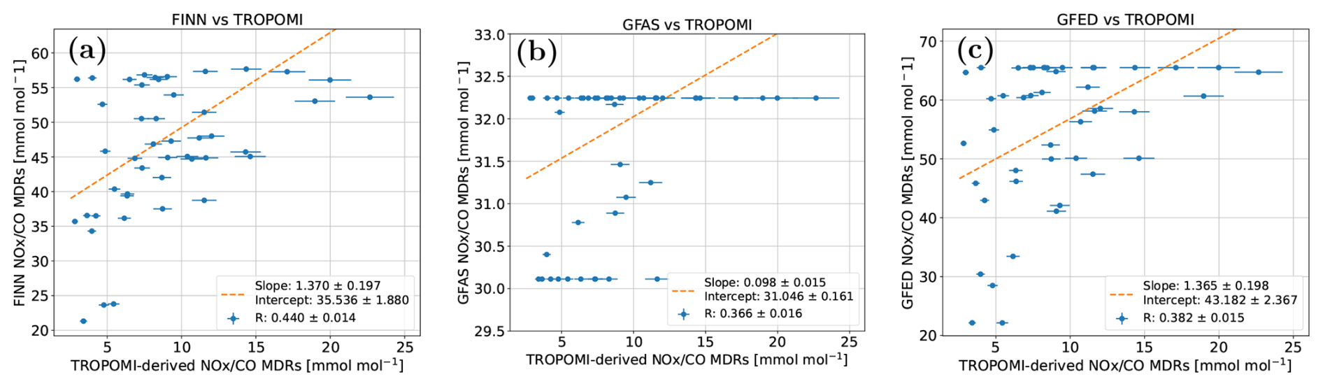
Figure 12 TROPOMI vs inventories correlation between NO_x and CO emission rates for (a) FINN, (b) GFAS, and (c) GFED. The dashed orange line represents the linear fit. The TROPOMI data correspond to MDRs applying a NO₂-to-NO_x factor of 1.4. The error bars in the TROPOMI data cover the 1.3–1.5 range for the NO₂-to-NO_x factor.

5.2.3 Assessment of TROPOMI and inventory-based NO_x $/$ CO MDR

We also assess the correlations between TROPOMI and inventories NO_x $/$ CO MDR. The results are shown in Fig. 12.

As shown in Fig. 12, the NO_x $/$ CO MDR inferred from satellite observations are in general a factor of 2–4 smaller than those from inventories. This offset is consistent with the finding that TROPOMI-derived CO emissions are about a factor of 3 higher than the inventory estimates. The lower TROPOMI-derived NO_x $/$ CO ratios therefore mainly point to an underestimation of CO in the inventories rather than to an underestimation of NO_x by the satellite-based method. This also provides confidence in the combined plume-masking and mass-balance approach, because a systematic methodological low bias would be expected to affect both species more similarly. Nevertheless, NO₂-specific retrieval and chemical effects may also influence our TROPOMI-derived MDRs. Sensitivity tests show that expanding the NO₂-to-NO_x scaling factor from the reference 1.3–1.5 range to 1–2, increases the spread of the satellite MDRs but does not remove the systematic difference from the inventories (Sect. S3). Similarly, restricting the MDR calculation to the pixels closer to the hot spot (i.e, fresh plume) gives a slope close to unity relative to the full-plume calculation, indicating no significant systematic effect of plume ageing at the spatial scales considered here. Moreover, moderate scattering-related possible NO₂ perturbation experiment also yields little systematic change in the MDR, although individual cases are more variable (Sect. S1.2).

The three inventories show different behaviour in this comparison. GFAS exhibits almost no variability in NO_x $/$ CO ratios across the analysed fires, with most values clustering around a small number of discrete levels. This suggests that GFAS applies relatively fixed emission-ratio assumptions for the relevant fire categories as discussed in Sect. 5.2.2. In contrast, both FINN and GFED show a broader range of NO_x $/$ CO ratios, more similar to the variability seen in the TROPOMI-derived ratios. Figure 12 also shows an apparent upper limit in the inventory-derived NO_x $/$ CO MDRs, at approximately 55 mmol mol⁻¹ for FINN, 32 mmol mol⁻¹ for GFAS and 65 mmol mol⁻¹ for GFED. This is consistent with the finite range of NO_x $/$ CO ratios implied by the biome-specific emission factors used by each inventory (Table 3).

The correlations between TROPOMI and the inventories are weak but positive, with the highest correlation for FINN (R=0.45), followed by GFED (R=0.39) and GFAS (R=0.37). This indicates that, despite the absolute offset, FINN and GFED capture part of the relative variability in emission ratios among fires. Such variability is likely linked to differences in vegetation type, fuel properties or combustion conditions. The fact that TROPOMI retrieves a similar tendency without explicit prior information on biome type supports the interpretation that the satellite-derived ratios contain independent information on fire variability.

Figure 13 Temporal evolution of two wildfires for different hotspots. (a) #1 (Jarilla) covering 5 d and (b) #10 (Arganil) covering 11 d. Top panels show the CO emission rates (t h⁻¹), while in lower panels show the NO_x $/$ CO MDRs. TROPOMI-related values are shown in red, GFAS' in blue, GFED's in orange and FINN's in green. The red shadow of lower panels corresponds to the TROPOMI NO_x $/$ CO MDR using different NO₂-to-NO_x conversion factors (Sect. 4.3).

5.3 Temporal evolution of selected fire emissions

Based on the number of satellite overpasses and the performance of the plume masking, the temporal evolution of two specific wildfires was also analysed in order to investigate their particular dynamics of CO emission evolution during their lifetime and the NO_x $/$ CO MDR. These time-evolutions are investigated from TROPOMI observations and from inventories (GFAS, GFED, FINN) perspective.

Figure 13 shows these time-evolutions for the selected wildfires: Arganil (Portugal, evolution during 11 d; #10) and Jarilla (Spain, evolution during 5 d; #1). Note that, based on the Portuguese Institute for Nature Conservation and Forests (ICNF, 2025), in terms of area burned, Arganil's wildfire ended up being one of the largest wildfires in Portugal in the last decade. Figure S18 of the Supplement shows a satellite perspective of the different overpasses above the wildfire of Arganil (site #10 of Table 1), showing not only the evolution of that fire but also how other hotspots surrounded Arganil.

The comparison of the temporal evolution of CO emission rates (upper plots in Fig. 13) shows that, while inventories reproduce similar magnitude as the observations, the agreement is event and time-dependent. Observations in Jarilla (#1, Fig. 13a) suggest a strong CO emission peak on 17 August, not fully captured by inventories. In the case of Arganil (#10, Fig. 13b), observations suggest a strong CO emission peak on 15 August and a second elevated period (19–22 August). The inventories reproduced only partially this episodic evolution, with relevant differences between inventories. In particular, for Arganil, GFAS reports a similar peak CO emission rate as the observations, but one day later than observations.

Regarding the time-evolution of the NO_x $/$ CO MDR, the different temporal behaviour between inventories and TROPOMI MDR is also important (Fig. 13, bottom panels). In the case of Arganil wildfire (#10), TROPOMI MDR shows a broad fire mid-life depression, whereas GFAS estimates are nearly flat. Although in different absolute values, MDR of GFED and FINN also show a high-low-high time evolution as TROPOMI, suggesting these three sources capture somehow similar plume ageing and combustion efficiency. A similar scenario is shown for the MDR time evolution in Jarilla (#1). While TROPOMI, GFED and FINN MDR estimates show a rather (relative) consistency in time evolution, GFAS provides constant MDR values.

In general, for these two fires and as mentioned in Sect. 5.2.3, NO_x $/$ CO MDR derived from TROPOMI observations show consistently lower MDR throughout the lifetime of the fires. This result may indicate that the inventory EF ratios are too high for the conditions sampled in these fires, or may be consistent with comparatively CO-rich combustion conditions, including a larger contribution from smoldering combustion at some stages of the fires. Firefighting intervention may also influence the temporal evolution and combustion conditions of individual fires. Such activities are not explicitly represented in the emission inventories used in this work, although their effects may be indirectly reflected in the satellite fire observations on which those inventories rely. In contrast, the atmospheric columns observed by TROPOMI at the overpass time integrate the actual state of the plume and therefore may also reflect any preceding influence of firefighting activities on the fire emissions. However, the effect of firefighting activities cannot be evaluated with the information available. In general, the MDR comparison is not direct: inventories report emitted NO_x and CO, whereas TROPOMI samples downwind NO₂ and CO. Chemical ageing of NO_x or the NO₂-to-NO_x factor assumed herein may also influence the different timing found.

Overall, this wildfire time evolution exercise suggests that the comparison of TROPOMI and inventories emission rates or MDR cannot be reduced to a single scaling factor. Also, although the overall CO flux magnitudes may agree, they might show a time or individual event mismatch. In general, the temporal evolution of the NO_x $/$ CO MDR inferred from TROPOMI data is partly reproduced by GFED and FINN, however GFAS shows little to none MDR time variability. These results highlight the potential of TROPOMI to constrain fire emission estimates but also the need to consider temporal sampling, plume chemistry and the EFs assumed by each inventory for the burned vegetation when comparing with inventories.

6 Conclusions

Summer 2025 was an exceptional wildfire season in southern Europe, marked by record fire activity and emissions across the Iberian Peninsula, particularly during the severe August wildfires in Spain and Portugal. During that month, a devastating fire scene took place with over 100 wildfires declared in Spain, nearly 80 fires in Portugal. Those August 2025 fires in the Iberian Peninsula emitted about 1 Mt of CO, representing 50 % of the cumulative CO wildfire emissions estimated for the European Union in 2025 (EFFIS, 2026).

This study provides a satellite perspective of this fire season from the CO emissions point of view. In particular, we report on CO emission estimates inferred from TROPOMI observations of the northwestern region of the Iberian Peninsula during August 2025. The study covers up to 15 wildfires that ended up burning 70 % of the total area burned in the Iberian Peninsula during that month. Overall, we report on 46 individual top-down assessments of CO fluxes, providing not only event-scale CO emission estimates but also information on the temporal evolution of some fires. This includes the Arganil fire in Portugal, one of the largest wildfires on record in the country, for which emissions could be followed over an 11 d period. Our satellite-based CO emission estimates were compared to those inferred from three widely used fire emission inventories (FINNv2.5, GFASv1.2 and GFEDv5.1). Although the comparison shows considerable variability, TROPOMI-derived CO emissions were about three times higher than those from inventories, suggesting a systematic low bias in these inventories for the fires studied herein. Results also indicate that inventories do not seem to reproduce the CO emission peaks detected by TROPOMI. Sensitivity tests indicate that this systematic difference cannot be explained by any of the individual methodological choices tested in this work. Our results are therefore consistent with a low bias in inventory CO emissions for the fires and sampling conditions investigated, although differences in temporal sampling and other unresolved sources of uncertainty may also contribute to the observed offset.

In addition to top-down CO emission rates, we also report on satellite-derived NO₂ $/$ CO mole density ratio perspective of the observed fires, providing complementary information on plume composition. Our results, segregated by regions, show a great variability on those ratios, from 2.4 to 9.8 mmol mol⁻¹, suggesting differences in fuel type and combustion conditions. The Portuguese fires showed the lowest ratios, possibly more forest-related burning, while the Zamora–León fires in Spain showed higher and more coherent NO₂ $/$ CO ratios, indicative of relatively NO₂-rich plumes and a possible stronger flaming contribution. Together with the MODIS land-cover information, these results suggest that the fires mainly affected Mediterranean vegetation, while retaining distinct regional signatures. Furthermore, we scale these satellite NO₂ $/$ CO MDR to NO_x $/$ CO MDR and compare also with inventories. In agreement with the found CO fluxes underestimation of the inventories, the absolute NO_x $/$ CO MDR from TROPOMI were smaller than inventories. At the same time, the weak but positive correlations of TROPOMI-based NO_x $/$ CO MDR with FINN and GFED MDR indicate that these inventories capture part of the relative variability between fires, likely through biome- or fire-type-dependent EFs. GFAS, in contrast, shows much less variability, highlighting the influence of inventory-specific assumptions on emission-ratio estimates. Overall, time-dependent relative plume composition during the lifecycle of the two fires investigated herein is partly resolved in some of the emission inventories (GFED, FINN).

From satellite observation perspective, one particular challenge found throughout this work was to differentiate individual plumes under multi-fire conditions. This was particularly relevant during the August 2025 Iberian fires, when several active fire fronts were located close to each other and their plumes partly overlapped. This plume overlap is common during extreme wildfire episodes, making the attribution of satellite-derived emissions to individual fires more uncertain. To address this complexity, we introduced a fresh-plume masking approach based on collocated satellite NO₂ observations, which enabled us to identify source-specific CO plumes and support the attribution of CO emissions to individual fires. However, in cases with complex wind fields and strongly overlapping plumes, this synergy mask was still not sufficient to fully separate all the individual fire contributions. This remains a broader challenge for satellite-based fire-emission studies, especially in extreme multi-fire situations where nearby sources and changing winds make plume attribution difficult.

Overall, these results demonstrate that satellite observations can provide independent constraints not only on the magnitude of fire emissions, but also on the emission ratios that shape their atmospheric-chemistry impact. While inventory estimates depend on assumptions about burned area, fuel consumption and EFs, the combined analysis of TROPOMI CO and NO₂ enables an inventory-independent quantification of emission rates and emission ratios at the plume scale.

Beyond the 2025 Iberian wildfires, this study shows the benefit of combining satellite observations from different spectral ranges, not only to study relationships between atmospheric species, but also to analyse complex emission scenes by taking advantage of the different chemical lifetimes and complementary spatial information. This type of multi-species approach is relevant for current and forthcoming atmospheric composition missions, from Sentinel 5P and Sentinel 5 to CO2M, where complementary trace gas observations are increasingly used to improve plume detection, source attribution and emission quantification. It also provides a useful framework for future distributed small satellite concepts such as the Spanish ANSER-AT mission, where observations from different CubeSats in different spectral windows are expected to provide complementary information on atmospheric species.