New insights into urban ethanol and oxygenated volatile organic compound sources from combined flux tower and mobile measurements

Oxygenated volatile organic compounds (OVOCs) including ethanol, methanol, acetone, and acetaldehyde are important components of urban VOC emissions, yet their sources and emissions magnitudes remain highly uncertain. In this study, we leveraged data from a Vocus proton-transfer reaction mass spectrometer deployed during a long-term tower-based eddy covariance flux study and a mobile monitoring campaign to characterize the emissions and sources of urban OVOCs. Ethanol accounted for about half of the measured molar flux and a fifth of the calculated OH reactivity flux. A tracer-based source apportionment approach revealed that cooking was the predominant source of ethanol in the flux footprint (63 % of the ethanol flux), followed by volatile chemical products (VCPs) and other sources (28 %), and motor vehicles (9 %). This result supports the recent inclusion of cooking in VOC emissions inventories and further supports indoor environments as important contributors to urban atmospheric chemistry. Cooking was also a major source of acetaldehyde, while VCPs were the main sources of acetone and methanol in the flux footprint. Mobile monitoring within the flux footprint and beyond informed the representativeness of the tower-based measurements and identified additional OVOC sources. In the broader urban region, fossil fuel combustion was a key source of acetaldehyde, and industrial zones and waste treatment facilities missed by the flux tower were hotspots for ethanol, methanol, and acetone emissions. Together, these results provide new constraints on the sources, seasonality, and magnitude of OVOC fluxes in urban environments through a unique synthesis of tower-based and mobile measurements.

1 Introduction

Chemical reactions in the atmosphere involving volatile organic compounds (VOCs) and nitrogen oxides (NO_x) lead to the formation of air pollutants including secondary organic aerosol (SOA) and ozone (O₃), components of photochemical smog that are damaging to human health (Pozzer et al., 2023). Air quality has improved dramatically in the United States (U.S.) since the 1970s due to the Clean Air Act and motor vehicle regulations, but some U.S. cities have recently experienced stagnated or reversed air pollution levels (Nassau and Jaeglé, 2025; Rosanka and Carlton, 2025; Warneke et al., 2012). Accurately describing VOC and NO_x emissions is a key part of understanding the formation and evolution of SOA and O₃. However, there are persistent uncertainties in modeling these secondary pollutants due in part to the complex chemical and physical processes driving their formation and the diverse array of VOC precursors.

VOCs have numerous anthropogenic and biogenic sources in urban areas. Volatile chemical products (VCPs), which include solvents, adhesives, and other consumer products, now emit more VOC mass and contribute more to SOA and O₃ formation than motor vehicle sources in U.S. cities (Gkatzelis et al., 2021; McDonald et al., 2018; Stockwell et al., 2025). Cooking has also recently emerged as an important source of VOCs in urban areas (Coggon et al., 2024a; Stockwell et al., 2025; Zhu et al., 2025). Despite recent advances in our understanding of urban VOC emissions, key uncertainties and disagreements with existing emissions inventories impede our ability to accurately model and predict air pollution.

Oxygenated VOCs (OVOCs) constitute a major fraction of reactive carbon in urban air and originate from effectively every source category including mobile sources, VCPs, vegetation, cooking, and more. Field measurements in cities across the Northern Hemisphere agree that OVOCs are the top contributor to observed VOC fluxes, mixing ratios, and reactivity (Acton et al., 2020; Li et al., 2022; Pfannerstill et al., 2023; Qian et al., 2025; Rantala et al., 2016). There have been substantial disagreements between OVOC flux measurements and emissions inventories in urban areas (Karl et al., 2018; Pfannerstill et al., 2023), highlighting a persistent knowledge gap in the sources of urban and regional air pollution.

Atmospheric ethanol (C₂H₅OH) is present at high concentrations in urban environments (Gkatzelis et al., 2021; Li et al., 2024, 2022; Millet et al., 2005). Globally, biogenic activity and decomposition are the dominant sources of ethanol (Naik et al., 2010). The use of ethanol as a fuel additive was associated with rising ambient concentrations in the 2000s and 2010s (de Gouw et al., 2012; Millet et al., 2012; Willey et al., 2019), though recent analyses attribute less than 20 % of ethanol emissions to mobile sources (Gkatzelis et al., 2021; McDonald et al., 2018). Indoor air is enriched in ethanol due to emissions from cooking, continuous indoor sources (i.e., building materials, VCPs), alcohol consumption, and consumer product use, and these emissions are ultimately transported outdoors (Arata et al., 2026; Liu et al., 2019; Nazaroff and Weschler, 2024). Despite its ubiquity, ethanol is considered to have significant missing sources in urban environments, which may include cooking, indoor to outdoor transport, and others (Pfannerstill et al., 2023). Ethanol is important for air quality because it reacts with hydroxyl radicals to form acetaldehyde with a high molar yield, which can further react to form peroxyacetic nitric anhydride, also known as PAN. PAN serves as a reservoir for long-range transport of NO_x, thus linking ethanol emissions to the NO_x cycle and ozone formation far from its emission sources (Fischer et al., 2014).

Other small (i.e., 1 to 3 carbon) OVOCs including methanol, acetaldehyde, and acetone are also important components of urban VOC emissions. These three compounds are among the most abundant VOCs in urban areas (Acton et al., 2020; Li et al., 2022; Velasco et al., 2009). Methanol is one of the most abundant VOCs globally due to its biogenic and secondary sources (Bates et al., 2021), but anthropogenic emissions from VCPs are thought to be the predominant source in urban areas (Velasco et al., 2009). Similarly, the main sources of global acetaldehyde and acetone are photochemical production and vegetation. Fossil fuel combustion and VCPs are the major anthropogenic sources of acetaldehyde and acetone, respectively (Gkatzelis et al., 2021). Like ethanol, indoor environments have high concentrations of acetaldehyde and methanol, with indoor-to-outdoor exchange influencing outdoor mixing ratios (Arata et al., 2026; Salthammer, 2023) and PAN formation (Fischer et al., 2014). Additionally, acetaldehyde and methanol are considered hazardous air pollutants by the Environmental Protection Agency (EPA).

The URBAN-EC project (Urban Research on Biogenic and ANthropogenic Emissions of Carbon) involved flux measurements at a tower site in Berkeley, California in the San Francisco Bay Area for 1.5 years to better understand sources of VOCs and greenhouse gases in urban environments. This manuscript combines VOC flux data from the tower-based study in addition to mobile measurements of VOCs collected within the tower footprint and beyond to elucidate key sources and drivers of VOC emissions in urban areas. VOC fluxes were calculated using the eddy covariance method and provide a direct measurement of emission and deposition rates for all hours of the day across all four seasons. Mobile measurements, while not as temporally rich, provide the spatial distribution and chemical fingerprint of VOC hotspots and a measure of the representativeness of the URBAN-EC fluxes within the broader Bay Area. We identified VOCs with the highest measured mixing ratios, largest fluxes, and greatest contribution to the calculated OH reactivity flux. In all cases, OVOCs dominated. The integration of these datasets provides novel insights into the sources of atmospheric ethanol and other small OVOCs in urban environments.

2 Methods

2.1 Mobile measurements

2.1.1 Mobile measurements: Measurement details

The goal of the mobile monitoring campaign was to identify prominent urban VOC sources, and to this end, a non-targeted sampling approach was employed. A mobile sampling platform was equipped with trace gas and meteorological instruments including a Vocus proton transfer reaction time of flight mass spectrometer (Vocus PTR-ToF-MS, Aerodyne Research Inc.) which measured VOC mixing ratios and a MetOne sonic anemometer which measured wind speed and direction. Vehicle speed, direction, and location were tracked using iPhone GPS apps. The Vocus sampled ambient air through filtered (47 mm PTFE membrane filters with 2 µm hole size) 0.32 cm inner diameter Teflon tubing at ∼ 2 L min⁻¹. The inlet tubing was mounted approximately half a meter above the van roof with the inlet facing away from the exhaust. Inlet tubing was ∼ 3.8 m long.

Mobile measurements were conducted in November of 2021 and January and February of 2022. 12 d of mobile data are included in this analysis. These days had similar meteorological conditions (Table S1 in the Supplement) and rain was not reported during sampling. Measurements were made on weekdays during business hours (between 09:00 and 17:00 LT), so as a result, the study is biased to emissions occurring during these hours. The sampling domain transected multiple neighborhood sizes and types (industrial, commercial, and residential) and encompassed two domains: most of Berkeley, California and part of Oakland, California. Roughly, the same roads were sampled on each day for each domain, and measurements were randomized in terms of street sampling order and sampling time. Sampling covered numerous road types including major highways, major arterial roads, and minor side streets. The mobile sampling domain included the flux tower footprint (Fig. 1, area of influence for flux measurements, discussed below).

2.1.2 Mobile measurements: Instrumentation and calibrations

The Vocus is a chemical ionization mass spectrometer which uses hydronium ions (H₃O⁺) to ionize the analytes via proton transfer. The Vocus has a focusing ion molecular reactor (FIMR) which improves sensitivity by focusing H₃O⁺ and molecular reagents (VOCs) into a narrow beam. The Vocus is described in more detail by Krechmer et al. (2018). While the PTR-MS is typically considered a soft ionization technique, some fragmentation can occur. The degree of fragmentation is modulated by the $\mathrm{E}/\mathrm{N}$ ratio (i.e., the ratio of the electric field to gas number concentration) and other voltages in the FIMR. For example, isoprene was not calibrated in the mobile dataset because of interferences from fragmentation and lack of data to perform the correction.

Calibrations were performed approximately every 2–4 h using two gravimetrically prepared cylinders (Apel Riemer). Zero air was generated using a platinum catalyst and was used to dilute air from the cylinders in multipoint calibrations (3–4 points). Calibration factors and zeros were stable (within 10 %) throughout the measurements each day, so one set of calibration factors and instrument zeros were used for each day. Well-behaved calibrants are those that do not fragment or those whose fragmentation products may be summed with confidence, such as monoterpenes (C₁₀H${}_{\mathrm{17}}^{+}$ + C₆H${}_{\mathrm{9}}^{+}$). Well-behaved calibrants have a linear relationship with the proton transfer reaction rate constant (k_PTR). The linear relationship between well-behaved calibrants and k_PTR was calculated for each day, and a default sensitivity was calculated as a ratio of this linear relationship and a k_PTR of 2.25 × 10⁻⁹ cm³ molecule⁻¹ s⁻¹. On average, the default sensitivity was 5500 (4600–8400) counts per second (cps) per ppb. The uncertainty range is based on the possible k_PTR values for ambient VOCs, 1.85 to 3.39 cm³ s⁻¹ molecule⁻¹ (Holzinger et al., 2019). The default sensitivity was used to calibrate VOCs not in the calibration standards.

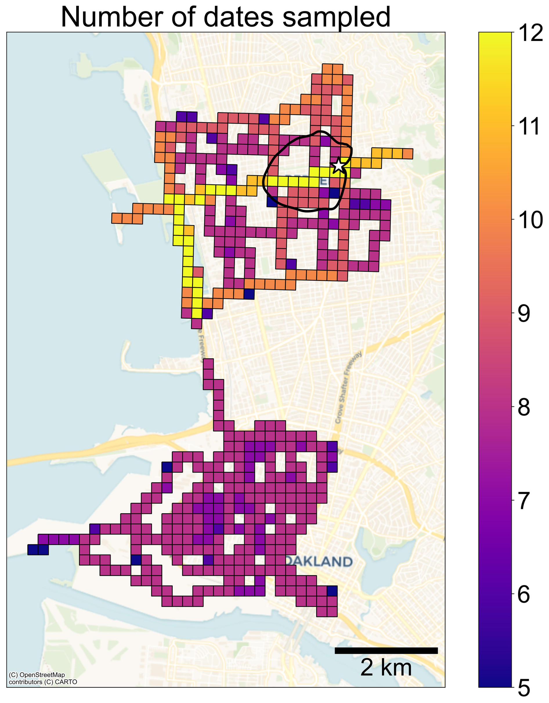
Figure 1 200 m by 200 m grid cells colored by the number of unique dates mobile measurements occurred. The black trace is the 80 % flux footprint, and the white star is the location of the URBAN-EC flux tower. Map data © OpenStreetMap contributors, distributed under the Open Data Commons Open Database License.

2.1.3 Mobile measurements: Data analysis

Mobile data was gridded so that measurements taken at the same location on different days could be analyzed together. Gridded data was used to assess neighborhood scale gradients and identify persistent hotspots of VOC emissions. This dimensionality reduction approach is in line with previous work by Apte et al. (2017). Each grid cell was 200 m by 200 m, roughly the length of one city block. Grid cells were included in the analysis if they were sampled on at least five different dates (Fig. 1). Grid cells were visited one or two distinct times per day, and there were multiple data points per visit since data was collected at 1 Hz. For each grid cell, the median of daily means is presented. The relative standard deviation (RSD = ratio of standard deviation to mean) of daily means for each grid cell was ∼ 50 % for most grid cells (Fig. S1 in the Supplement). Generally, regions identified as hotspots for VOC emission in this analysis did not coincide with regions with high RSDs, reflecting the robustness of the results (Fig. S2). Some regions had RSDs higher than 50 % but were not central components of the discussion and analysis. These high RSD areas represent locations with sporadic emission events.

Spikes in VOC concentration were identified using background-subtracted data. The background concentration for each VOC was designated as the 10th percentile in 10 min rolling windows. Background subtracted data were only used for spike identification and were not used to present quantitative metrics throughout the manuscript. We considered designating the background as the 5th percentile, similar to Apte et al. (2017), but the differences were negligible. Spikes were defined as 1 Hz data points above the 95th percentile in 10 min windows. 1 Hz spike data points within 1 min were aggregated so that each spike was assigned one data point. Figure S3 demonstrates where spikes were identified for a representative sample. For a given VOC, spike co-occurrences were found by calculating VOC correlations within an 8 s window around each spike. VOCs with correlations (R²) above 0.85 in this window were considered coincident. Figure S4 demonstrates how VOC correlations were found around each aggregated spike data point. Known fragments and water clusters were omitted from the correlation analysis. C₁₀H${}_{\mathrm{17}}^{+}$, the formula for protonated monoterpenes, could have been impacted by fragmentation of monoterpenoids. Also, C₆H${}_{\mathrm{7}}^{+}$, the formula for protonated benzene used in the mobile dataset, may be influenced by fragmentation of substituted aromatic VOCs.

2.2 Tower measurements

2.2.1 Tower measurements: Measurement details

A flux tower was established for long-term measurements in March 2022 at the Berkeley Way West building in downtown Berkeley, California. The project, URBAN-EC, was introduced and described in detail by Katz et al. (2025), who analyzed data collected between May and November 2022. This dataset builds off that work. Briefly, the tower was a telescoping mast (Floatograph FM50) set 10 m above the roof and 40 m above the ground. Instruments were housed in a small room on the roof, and ∼ 35 m of heated, filtered, Teflon inlet tubing (0.32 cm inner diameter) ran from the top of the tower to the instruments. The tubing flow rate was set to 10 L min⁻¹, which resulted in residence times under 3 s. VOC mixing ratios were measured at 10 Hz using a Vocus PTR-ToF-MS between May 2022 and April 2024. 3D wind was measured at 20 Hz by a sonic anemometer (Gill Windmaster) during this time. Continuous Vocus data was available from May to November 2022, April 2023 to January 2024, and in March 2024. The full URBAN-EC VOC dataset includes measurements from 16 complete months and all four seasons. Monthly statistics are shown if data collection occurred for at least 50 % of the month.

2.2.2 Tower measurements: Instrumentation and calibrations

The same Vocus PTR-ToF-MS from the mobile study was used at the flux tower. One set of operating conditions was used from May to November 2022, one set was used for April 2023 to January 2024, and one set was used in March 2024. We discuss these differences and the impact on the measurements below. Calibrations and zeros were performed once to three times daily and interpolated across the dataset. Gravimetrically prepared calibration cylinders were used (Apel Riemer). Sesquiterpenes (C₁₅H${}_{\mathrm{25}}^{+}$), nonanal (C₉H₁₉O⁺), and octanal (C₈H₁₇O⁺) were calibrated using the default calibration factor scaled by the fraction of parent ion detected in laboratory calibrations (Katz et al., 2025). Thus, these VOCs were calibrated using the default sensitivity accounting for instrument-specific fragmentation patterns. These ions, along with propanol (dehydration product: C₃H${}_{\mathrm{7}}^{+}$), were not included in data from March 2024 because a standard was not available. The default sensitivity was found using the same method as the mobile data (Sect. 2.1.2) and applied to non-calibrant VOCs. See Katz et al. (2025) for additional details. The uncertainty of VOCs calibrated directly in the Vocus was 10 %, while it was 50 % for VOCs calibrated using the default sensitivity. The OVOCs highlighted in this study were calibrated directly. The influence of isobaric interferences on the compounds of interest could not be quantified. Fluxes of C₃H₇O⁺ were assumed to be predominantly from acetone, though some influence from propanal was possible. Reports of propanal fluxes in urban areas are sparse. In Beijing, the emission ratio of propanal (relative to acetylene) was ∼ 4 % of the emission ratio of acetone, while background concentrations of propanal were ∼ 16 % of acetone concentrations (Yuan et al., 2012). Together, these comparisons indicate direct emissions of propanal in urban areas are likely minimal relative to acetone, while regional transport or photochemical production could influence the observed C₃H₇O⁺ mixing ratios by up to 15 to 20 %. The mass to charge ($m/z$) range of the Vocus was 10 to 497. The sampling rate was 10 Hz. The FIMR was 100 °C and 2.5 mbar. The reagent flow was 15 standard cubic centimeters per second, the electric field gradient was 590 V, and the radio frequency was 450 V. The $\mathrm{E}/\mathrm{N}$ ratio was ∼ 125 Td (1 Td = 10⁻²¹ V m²). The big, segmented quadrupole (BSQ) voltage was 200 V. The sensitivities of the four OVOCs of interest are shown in Fig. S5.

Fragmentation can impact the detection of isoprene, benzene, and other VOCs in the Vocus. Coggon et al. (2024b) proposed a fragmentation correction for isoprene which utilizes the ions C₈H${}_{\mathrm{15}}^{+}$ and C₉H${}_{\mathrm{17}}^{+}$. In this dataset, isoprene fragmentation was corrected using these ions for data collected from April 2023 to January 2024. For data collected from May to November 2022 and March 2024, C₆H${}_{\mathrm{11}}^{+}$ was also used. When a large skimmer gradient (∼ 12 V) was used in the FIMR during 2022 and March 2024, an additional ion was needed to achieve an accurate isoprene correction and minimize overcorrection (time periods where isoprene was negative). Periods with a larger skimmer gradient were characterized by greater fragmentation despite having a similar $\mathrm{E}/\mathrm{N}$, and the greater degree of fragmentation may be why a third ion was needed in the correction. Katz et al. (2025) describe this correction in more detail and show external validation. From April 2023 to February 2024, a smaller skimmer gradient was used, and the original ions proposed by Coggon et al. (2024b) were used for the correction. For this dataset, benzene was calibrated directly using the charge transfer product (C₆H${}_{\mathrm{6}}^{+}$) instead of the proton transfer product (C₆H${}_{\mathrm{7}}^{+}$) to avoid issues with fragmentation. Propanol was calibrated on the dehydration product (C₃H${}_{\mathrm{7}}^{+}$); the proton transfer product was not detected in calibrations. Fragmentation of larger VOCs could influence the signal at C₃H${}_{\mathrm{7}}^{+}$ in addition to propanol, so it was not the focus of further analysis.

2.2.3 Tower measurements: Data analysis

Fluxes were calculated using the eddy covariance method, where fluxes are the covariance between concentration and vertical wind speed. InnFLUX (Striednig et al., 2020) was used to calculate fluxes at 30 min time resolution. The inputs included 20 Hz sonic anemometer data (3D wind, temperature, pressure, etc.) and up-sampled 10 Hz calibrated Vocus data. 90 ion formulas were included in this analysis. Katz et al. (2025) composed this mass list based on VOCs from the original Vocus mass list (660 formulas) which were above the flux limit of detection at least 50 % of the time. Quality assurance was performed on the full VOC flux dataset as described in Katz et al. (2025). Briefly, a stationarity test requirement of 60 % was used, a friction velocity (u^*) threshold of 0.2 m s⁻¹ was applied, and data from the East and Southeast were omitted because of the roof geometry (45–180°). All data are on Pacific Daylight Time (UTC −7 h). Lag times were determined for each VOC separately using the maximum covariance between vertical windspeed and mixing ratio for averaging intervals with high signal-to-noise ratios and interpolated across the dataset following a procedure in the InnFLUX code (described by Striednig et al., 2020). The flux noise root mean square error (RMSE), the most conservative estimate of flux noise, for the four OVOCs of interest was between 14 % and 16 % of the measured flux (median value) (Langford et al., 2015; Striednig et al., 2020).

Data were separated for seasonal analysis using meteorological definitions and include months with complete sampling: Spring (April 2023, May 2023), Summer (June 2022–2023, July 2022–2023, August 2022–2023), Autumn (September 2022–2023, October 2022–2023), Winter (December 2023, January 2024). November is excluded from Autumn statistics so 2022 and 2023 can be compared directly, as November is absent from the 2022 dataset. Also, November includes the start of the wet season in Berkeley and thus has different meteorological conditions compared to September and October. Weighted averages from the entire measurement campaign are the mean of monthly means weighted by the number of repeat sampling months. Daytime data, defined here as 07:00 to 21:00 LT, were primarily used in the analysis to focus on time periods with high turbulence, consistent wind directions, enhanced anthropogenic activity, and to capture both morning and evening rush hours.

Biogenic VOC emissions were modeled using the Model of Emissions of Aerosols and Gases from Nature (MEGAN) in single-point format (Guenther et al., 2012; Wang et al., 2022). The MEGAN model outputs presented by Katz et al. (2025) were used here (June to October 2022) to determine the influence of the biosphere on observed urban OVOC fluxes. MEGAN model inputs were measured directly at the site including photosynthetic photon flux density (PPFD), temperature, pressure, wind direction, and more. Leaf area index (LAI) was acquired from Sentinel-2 (European Space Agency, 2021).

Flux data were compared to the Greenhouse Gas and Air Pollutants Emissions System, GRA²PES (Lyu et al., 2024, 2025). GRA²PES comparisons presented here use August 2023 weekday emissions. GRA²PES December 2023 emissions were also considered but not included because there were only minor differences from August (Fig. S6). Month-to-month changes in emissions from VCPs and cooking in GRA²PES are from economic data and population density scalers, respectively, and do not reflect seasonal changes from meteorology. Weekday data from GRA²PES were used in the comparison, because for all OVOCs considered here, emissions reported in GRA²PES were less than 0.50 % different on weekdays compared to weekends. We compared measured fluxes to GRA²PES in three grid cells (four by four km each), including the grid cell containing the flux tower and two adjacent grid cells.

Flux footprints, which are the geographic area impacting tower measurements, were calculated using the methodology described by Kljun et al. (2015). Briefly, the footprint depends on the tower height, wind direction, wind speed, turbulence, stability, and surface roughness length, which was determined in 30° wind quadrants using Lidar scans. These parameters are described in more detail in the preceding publication (Katz et al., 2025). Flux footprint modeling, especially in urban environments, can be uncertain, so the intention with this analysis was to show the average geographic area of influence instead of to pinpoint exact emission sources on short time scales. Precipitation was measured at Lawrence Berkeley National Laboratory about 2.4 km from the flux tower (https://sites.google.com/a/lbl.gov/lbnl-meteorological-data/lbnl-weather-data, last access: 2 February 2025). Zoning data (e.g., residential, commercial, manufacturing) was acquired from the City of Berkeley (https://data.cityofberkeley.info/browse?q=Zoning+Districts &sortBy=alpha&pageSize=20&tags=planning, last access: 16 June 2025). Restaurant and bar data was scraped from Google Maps using the Apify console (https://console.apify.com/actors/2Mdma1N6Fd0y3QEjR/input, last access: 30 July 2025).

3 Results and Discussion

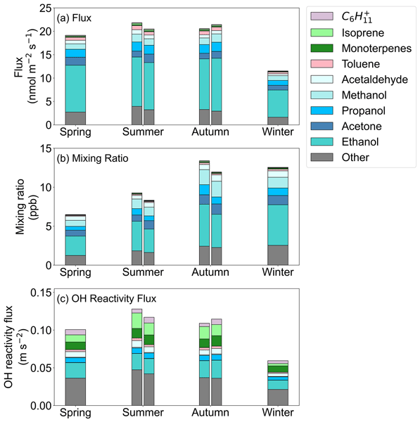
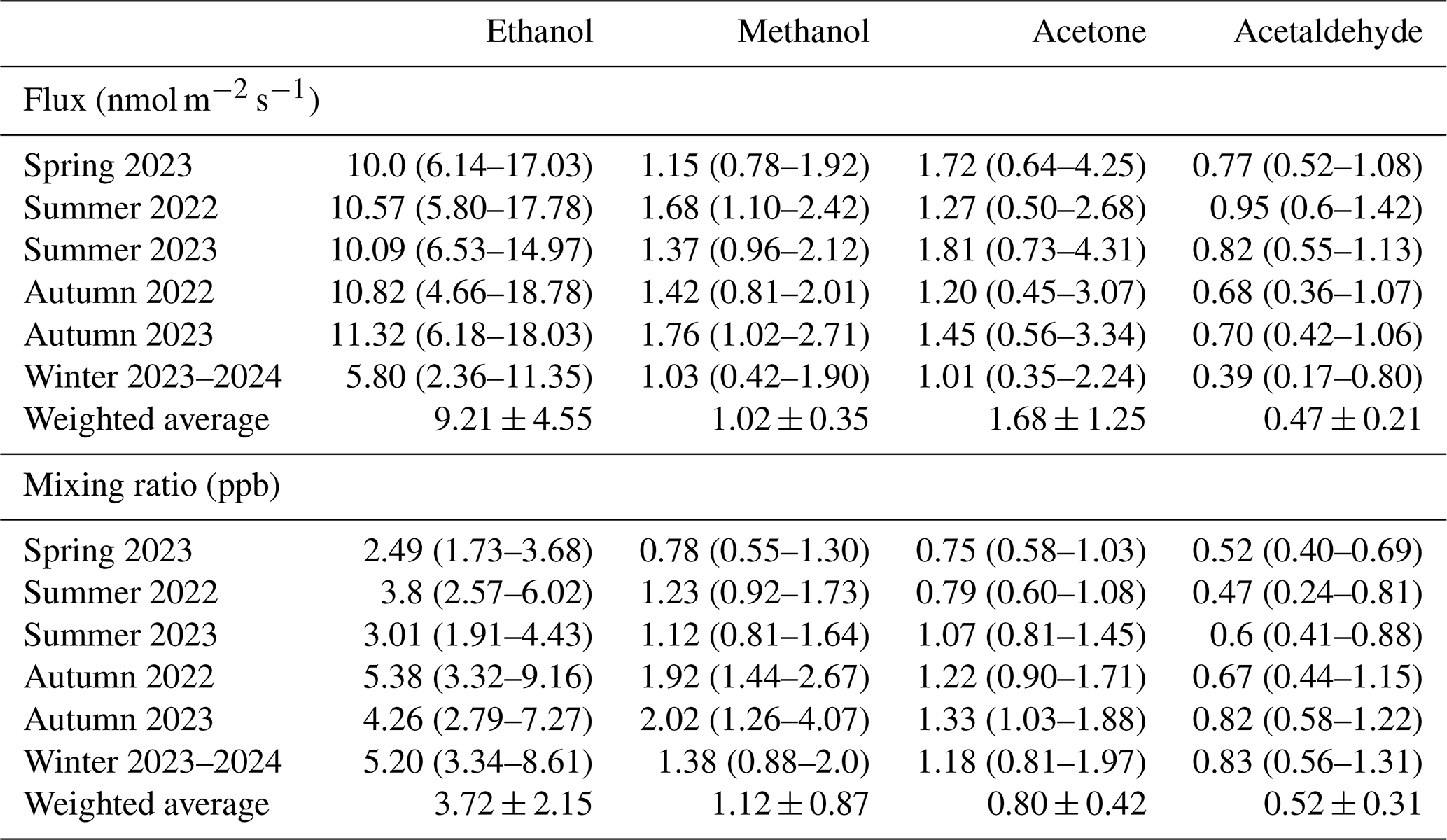
OVOCs dominated the total measured flux and mixing ratio during each season (Fig. 2). Ethanol was the greatest contributor to the measured flux, followed by acetone, methanol, and acetaldehyde. These four OVOCs accounted for 70 % of the measured flux, 69 % of the measured mixing ratio, and 27 % of the calculated OH reactivity flux. Because of their significance for the measured urban VOC flux, they are the focus of further analysis and source apportionment. Table 1 shows the median flux and mixing ratio of the OVOCs during each season and the weighted campaign average. Figure 3 shows meteorological data for each month. Figure S7 shows monthly mixing ratio data for each OVOC and ozone, and Fig. S8 shows median diurnal profiles of mixing ratio and flux for the key VOCs analyzed here. We looked for but did not observe a significant correlation between OVOC fluxes and temperature (Fig. S9), which may indicate that the trends in OVOC fluxes are predominantly driven by human activity.

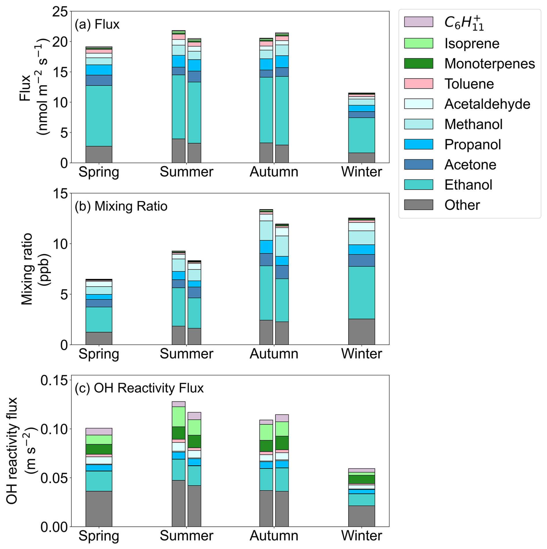
Figure 2 Daytime (07:00–21:00 LT) median VOC (a) measured molar flux, (b) measured mixing ratio, and (c) calculated OH reactivity flux for each season. The VOCs displayed are those that were present in the top 5 VOCs for any category (i.e., flux, mixing ratio, or OH reactivity) for at least one season. The VOCs are the same in each panel, and the stacking order is shown in the legend. Two bars are shown for summer and autumn, which represent sampling in 2022 (left) and 2023 (right). Spring sampling occurred in 2023, and winter sampling occurred in 2023–2024.

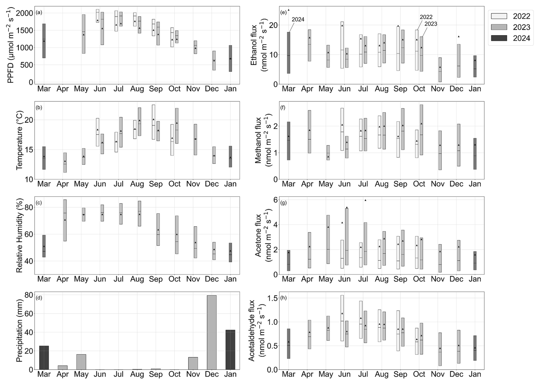
Figure 3 Monthly box plot of (a) photosynthetic photon flux density (PPFD), (b) temperature, (c) relative humidity (%), (d) precipitation, (e) ethanol flux, (f) methanol flux, (g) acetone flux, and (h) acetaldehyde flux at the URBAN-EC flux tower. Precipitation data is for 2023–2024. Data in (b), (c), and (e) through (h) include daytime hours (07:00 to 21:00 LT). Data in (a) include peak solar hours (10:00 to 14:00 LT). Boxes represent the interquartile range, the horizontal line within the box represents the median, and the triangle icon represents the mean. Precipitation is the total for each month.

Table 1 Daytime (07:00–21:00 LT) flux (nmol m⁻² s⁻¹) and mixing ratio (ppb) median and interquartile range (IQR, shown in parentheses) for ethanol, methanol, acetone, and acetaldehyde. Season definitions are described in Sect. 2.2.3. The weighted average and standard deviation of monthly averages are shown for the entire sampling period (described in Sect. 2.2.3).

3.1 Ethanol (C₂H₇O⁺)

Ethanol was 48 % to 53 % of the median measured molar flux, 17 % to 21 % of the calculated OH reactivity flux, and 36 % to 41 % of the measured mixing ratio across all seasons. Ethanol fluxes were about an order of magnitude higher than other OVOCs analyzed here. Ethanol fluxes were relatively stable throughout the year, though lower fluxes were observed from November through January and in May (Fig. 3). Lower fluxes during these months were most likely caused by lower local emissions. The exchange velocity (V_ex), the ratio of flux to concentration, was lowest in November through January (Fig. S10), while mixing ratios were highest during these months. This implies that the source strength in the flux footprint was relatively weaker, and that high mixing ratios were largely decoupled from processes within the flux footprint. The highest median ethanol flux was observed in autumn 2023 (11.32 nmol m⁻² s⁻¹) and the lowest flux was observed in winter 2023–2024 (5.80 nmol m⁻² s⁻¹) (Table 1). The campaign weighted average flux was 9.21 ± 4.55 nmol m⁻² s⁻¹ and the mixing ratio was 3.72 ± 2.15 ppb. Ethanol mixing ratios were the highest in autumn and winter (October to December) and lowest in May and June. Mixing ratios were predominantly driven by boundary layer dynamics. The mean mixing ratio and flux of ethanol was typically higher than the median, reflecting the importance of high, episodic emissions. Mean/median ratios for each month were between 1.2 and 2.6 for flux data, while mean/median ratios were between 1.2 and 2.1 for mixing ratio data. Net deposition (negative flux) was observed for 4.0 % of 30 min averaging intervals. There was minimal interannual variability for the months where two years of data are available (June through October), though fluxes were higher in June 2022 than June 2023. Ethanol fluxes in Berkeley were higher than observations from Beijing and Helsinki (Table S2), but seasonal cycles were consistent with those from Beijing (i.e., summer fluxes were higher than winter fluxes) (Acton et al., 2020; Rantala et al., 2016).

3.1.1 Tracer-based source apportionment: Ethanol

We assessed the source apportionment of ethanol using a tracer-based approach for known major source categories: fossil fuels, VCPs, cooking, vegetation, and decomposition. Biogenic fluxes of ethanol + acetaldehyde, an output of the single-point MEGAN model, were ∼ 500 times lower than observed ethanol fluxes, so biogenic ethanol emissions were assumed to be negligible in the footprint relative to other sources (Fig. S11). Ethanol emissions from decomposition were also assumed to be negligible in the footprint due to the lack of significant sources like composting facilities. Equation (1) describes the source apportionment approach for the remaining source categories, where F_EtOH is the flux of ethanol, F_EtOH,mobile is the flux of ethanol from motor vehicles, F_EtOH,cooking is the flux of ethanol from cooking, and F_EtOH,other is the flux of ethanol from indoor to outdoor transport, VCPs, and other miscellaneous sources.

$$\begin{array}{}\text{(1)}& F_{\mathrm{EtOH}}=F_{\mathrm{EtOH},\mathrm{mobile}}+F_{\mathrm{EtOH},\mathrm{cooking}}+F_{\mathrm{EtOH},\mathrm{other}}\end{array}$$

E10 gasoline (gasoline blended with 10 % ethanol) is used throughout California, and F_EtOH,mobile refers to ethanol emissions associated with this source. F_EtOH,mobile was calculated by multiplying the flux of benzene, F_benzene, by a scaling factor, S_EtOH,mobile (Eq. 2). S_EtOH,mobile was 7.1, which is the ratio of ethanol to benzene from on-road mobile sources in the GRA²PES inventory. F_EtOH,mobile is an upper-bound because it assumes all F_benzene originates from mobile sources which also produce ethanol. Diesel emissions, which are expected to be limited in the footprint relative to gasoline emissions, include benzene without ethanol. The median daytime F_EtOH,mobile was 9 % of the total ethanol flux.

$$\begin{array}{}\text{(2)}& F_{\mathrm{EtOH},\mathrm{mobile}}=S_{\mathrm{EtOH},\mathrm{mobile}}\cdot F_{\mathrm{benzene}}\end{array}$$

The flux of ethanol from cooking uses the same approach as F_EtOH,mobile, except with nonanal as the tracer for cooking emissions (Eq. 3). F_nonanal is the flux of nonanal and S_EtOH,cooking is the scaling factor for nonanal flux, i.e., the ratio of ethanol to nonanal during cooking. Nonanal is an established tracer for cooking emissions (Coggon et al., 2024a). To verify that nonanal is an appropriate tracer for cooking in the URBAN-EC footprint, the diurnal trend of nonanal flux is shown with the number of open restaurants per hour (Fig. 4). Nonanal fluxes were lowest on Sundays and Mondays when fewer restaurants were open, and they were highest during lunch (∼ 12:00 LT) and dinner (∼ 18:00 LT) hours with a lull around ∼ 15:00 LT when some restaurants closed. Thursdays, Fridays, and Saturdays had the highest nonanal fluxes and most restaurants open. The R² between the median nonanal flux per hour for each day of the week and the number of open restaurants was 0.81 (Fig. S12). The correlation indicates restaurants were a key source of nonanal in the footprint. Ethanol had a slightly weaker correlation with the number of restaurants open (R²=0.69), likely because ethanol had additional sources within the footprint besides cooking such as additional alcohol consumption on Thursday through Saturday evenings (discussed below) and VCPs.

$$\begin{array}{}\text{(3)}& F_{\mathrm{EtOH},\mathrm{cooking}}=S_{\mathrm{EtOH},\mathrm{cooking}}\cdot F_{\mathrm{nonanal}}\end{array}$$

The nonanal to ethanol ratios from cooking reported in the literature vary over two orders of magnitude. Ditto et al. (2023), who measured VOC emissions from cooking and cleaning in a restaurant, reported ethanol to nonanal ratios of 479 to 588. The ethanol to nonanal ratio for a cooking profile derived using positive matrix factorization of ambient VOC data was 11 (Coggon et al., 2024a). Also, Arata et al. (2021) measured indoor air at a test house during cooking experiments and reported an ethanol to nonanal ratio of 75. Indoors, other sources of nonanal could be present, such as surface ozone interactions and skin oil oxidation (Kruza et al., 2017), though we expect their influence to be minor in these studies because the ratios were taken during active cooking. We estimated S_EtOH,cooking ($\mathrm{ethanol}/\mathrm{nonanal}$) by examining the observed relationship between ethanol and nonanal when cooking emissions were sampled. Averaging intervals were assumed to be primarily influenced by cooking when nonanal/octanal was within 20 % of the observed nonanal/octanal ratio during dinner time (17:00–22:00 LT) and when benzene/ethanol was less than 0.01 to avoid influences from on-road sources. The scatter plot of ethanol versus nonanal during these times had a clear lower edge with positive ethanol scatter (Fig. S13). The lower edge without scatter indicates that nonanal was co-emitted with ethanol. Non-cooking sources of nonanal (e.g., surface ozone interactions) were expected to be negligible relative to cooking and likely did not influence the lower edge. S_EtOH,cooking was the slope of this lower edge and was found by fitting the 10th percentile of ethanol flux using the quantile regression approach (median $S_{\mathrm{EtOH},\mathrm{cooking}}=\mathrm{76}$, 95 % confidence interval = 70 to 82). The median value and the 95 % confidence interval (CI) were determined by bootstrapping the data. We sampled the data with replacement 10 000 times and calculated the slope of the lower edge of the ethanol versus nonanal scatter plot using quantile regression in each iteration. Figure S13 shows quantile regression results using the entire dataset.

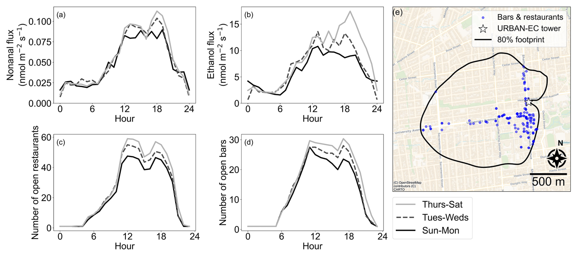
Figure 4 Diurnal plot of (a) median nonanal flux, (b) median ethanol flux, (c) the number of open restaurants per hour, and (d) the number of open bars per hour. Data are grouped by day of week: Sunday and Monday (Sun–Mon, solid black), Tuesday and Wednesday (Tues–Weds, dashed grey), and Thursday, Friday, and Saturday (Thurs–Sat, solid grey). Panel (e) shows the bars and restaurants within the 80 % flux footprint. Map data © OpenStreetMap contributors, distributed under the Open Data Commons Open Database License.

We tested the sensitivity of S_EtOH,cooking to a variety of factors. First, we performed the quantile regression using the 5th to 20th percentiles, which resulted in slopes ranging from 64 to 90 (average =77, standard deviation =9). Lower percentiles (20th and below) were chosen to capture the lower edge and because ethanol fluxes were influenced by sources in addition to cooking. We also considered binned linear fits through the 10th percentile of ethanol flux for certain subsets of the data, including selected wind sectors, dinner hours, and seasons. These conditions resulted in slopes ranging from 77 to 121. However, some subsets of the data (e.g., NW wind sector) had fewer data points available, which reduced the points available to define the lower edge, increasing the uncertainty. Considering each iteration, the average slope was 83 and the standard deviation was 12. The $\mathrm{ethanol}/\mathrm{nonanal}$ ratio we determined through quantile regression and bootstrapping ($S_{\mathrm{EtOH},\mathrm{cooking}}=\mathrm{76}$, 95 % CI = 70 to 82) is consistent with observations from cooking experiments at a test house ($\mathrm{ethanol}/\mathrm{nonanal}$ = 75, Arata et al., 2021), the GRA²PES inventory ($\mathrm{ethanol}/\mathrm{nonanal}$ = 110), and average of possible $\mathrm{ethanol}/\mathrm{nonanal}$ ratios from the additional cases tested from our dataset ($\mathrm{ethanol}/\mathrm{nonanal}$ = 83). Ethanol/nonanal likely varies with food and cooking methods, so this process was chosen to represent all cooking emissions within this flux footprint. With this scaler-based source apportionment approach, 63 % of the median daytime ethanol flux was attributed to cooking.

Day-of-week diurnal trends (Fig. 4) show that evening (17:00–21:00 LT) ethanol fluxes were significantly enhanced Thus-Sat relative to Sunday–Monday (p=0.0007) and Tuesday–Wednesday (p=0.02). Average evening ethanol fluxes were 90 % higher on Thursday–Saturday than Sunday–Monday, and average nonanal fluxes were 36 % higher. The flux footprint has a high density of bars and restaurants (Fig. 4, ∼ 80 bars and restaurants km⁻²), and 30 % more bars and restaurants were open Thursday–Saturday evenings than Sunday–Monday. It is plausible that the observed ethanol enhancements on Thursday–Saturday evenings were caused by alcoholic beverage consumption and cooking. Indoors, ethanol can reach exceptionally high concentrations (exceeding 1 ppm) when alcohol is consumed (Liu et al., 2019). Additionally, ethanol fluxes were 118 nmol m⁻² s⁻¹ in a German football stadium and were largely attributed to alcohol consumption, a magnitude about 10 times the ethanol flux observed here (Veres et al., 2013).

Ethanol fluxes from specific VCPs and other miscellaneous sources, F_EtOH,other, are more difficult to characterize via the tracer approach because of the multitude of potential sources and corresponding tracers. After quantifying ethanol emissions from fossil fuels and cooking, F_EtOH,other was calculated as the residual of the measured flux (Eq. 4). The median daytime F_EtOH,other was 28 % of the ethanol flux. About 30 % of averaging intervals were negative from either over-estimation of F_EtOH,mobile and F_EtOH,cooking or because of ethanol deposition. Most negative values were overnight; the fraction of negative F_EtOH,other was highest between 02:00 and 06:00 LT. Nonanal fluxes remained elevated overnight and potentially contributed to overestimating F_EtOH,cooking during these hours. This analysis focused primarily on daytime hours, 07:00 to 21:00 LT, so these time periods did not impact the interpretation.

$$\begin{array}{}\text{(4)}& F_{\mathrm{EtOH},\mathrm{other}}=F_{\mathrm{EtOH}}-(F_{\mathrm{EtOH},\mathrm{mobile}}+F_{\mathrm{EtOH},\mathrm{cooking}})\end{array}$$

Indoor to outdoor transport has been identified as a potential source of missing ethanol in urban areas. Indoors, ethanol has numerous sources and the concentration is typically higher than outdoors (indoor mean = 170 ppb) (Arata et al., 2021, 2026; Nazaroff and Weschler, 2024). Alcoholic beverage consumption, cooking, and cleaning are notable sources of episodic emissions, while continuous emissions from building materials and furnishings are also important (Liu et al., 2019). Nazaroff and Weschler (2024) estimated that the emission rate of ethanol from indoor residences to the outdoors is 640 mg d⁻¹ per person. Using the footprint population density of 6500 people km⁻² and median F_EtOH,other, we calculated an ethanol emission rate of 1500 mg d⁻¹ per person, which is within a factor of 2.3 of the estimate from Nazaroff and Weschler (2024). The per person emission rate from this study is most likely higher because F_EtOH,other accounts for all ethanol emissions besides vehicles and cooking. It likely includes contributions from outdoor VCPs, construction activities, and ethanol consumption at bars and restaurants, which are activities the estimate from Nazaroff and Weschler (2024) does not include. Further, the true daytime population density in the flux footprint is likely higher than the residential population density due to commuters.

Through this tracer-based source apportionment method, we attributed 63 % of median measured ethanol to cooking, 9 % to on-road sources, and 28 % to VCPs and other sources. Figure 5 shows the source apportionment for the three dominant wind sectors sampled: Northwest (NW), West (W), and Southwest (SW). The fraction attributed to cooking emissions was higher from the SW where there are more restaurants (Fig. 4). The source apportionment was similar in the W and NW, though NW had a higher contribution from other sources, likely because indoor to outdoor transport dominated the ethanol emissions in this residential area. The GRA²PES inventory attributed 63 % of ethanol emissions to cooking, 34 % to VCPs and 3 % to on-road, off-road, and industrial sources in the grid cell containing the flux tower (Fig. 5). Previous versions of this emissions inventory (FIVE-VCP, Harkins et al., 2021; McDonald et al., 2018) did not include cooking. The addition of this source improves the fractional comparison because cooking is a major source of ethanol in both GRA²PES and this study. We note that since F_EtOH,mobile was derived using the measured benzene flux and the ethanol/benzene ratio from GRA²PES, the comparison is not entirely independent. Positive matrix factorization of VOC mixing ratios in New York City attributed 17 % and 83 % of ethanol to mobile sources and VCPs, respectively (Gkatzelis et al., 2021). McDonald et al. (2018) report a similar breakdown in ethanol source apportionment. This work corroborates recent analyses by Coggon et al. (2024a) and Stockwell et al. (2025), who showed that cooking was a predominant source of VOCs in urban areas. This also supports results from Arata et al. (2026), who estimated that 25 % to 50 % of outdoor ethanol in the San Francisco Bay Area originates from indoor environments.

While our fractional source apportionment results agreed well with GRA²PES, the absolute magnitude of the ethanol emission in GRA²PES was 3.3 times higher than the median observations for our grid cell (Fig. 6). The neighboring grid cell to the North of the URBAN-EC tower, which has a lower population density, had better agreement. Population density and economic data are used to calculate cooking and VCP emissions in GRA²PES. This grid cell comparison indicates that population density scalers used to compute ethanol emissions in this region may be currently overestimated. Direct comparisons in neighboring grid cells with variable population densities would confirm this assumption. This grid cell and flux footprint are unique in that they have a high restaurant density, high population density, and large influx of commuters and students during the week. The high population density of the flux footprint could have contributed to the discrepancy with GRA²PES. Previous work on urban OVOC fluxes also found discrepancies between observations and emissions inventories (e.g., Acton et al., 2020; Karl et al., 2018). For example, Pfannerstill et al. (2023) found that ethanol was an important contributor to the measured mass flux (29 %) in Los Angeles, California, and that observations were substantially higher than the emissions inventory, FIVE-VCP. Cooking emissions were thought to be an important cause of the disagreement at that time. This study shows that cooking is a key source of ethanol in urban environments, and the updated GRA²PES inventory which includes cooking is a more robust description of ethanol emissions compared to previous estimates which did not include cooking.

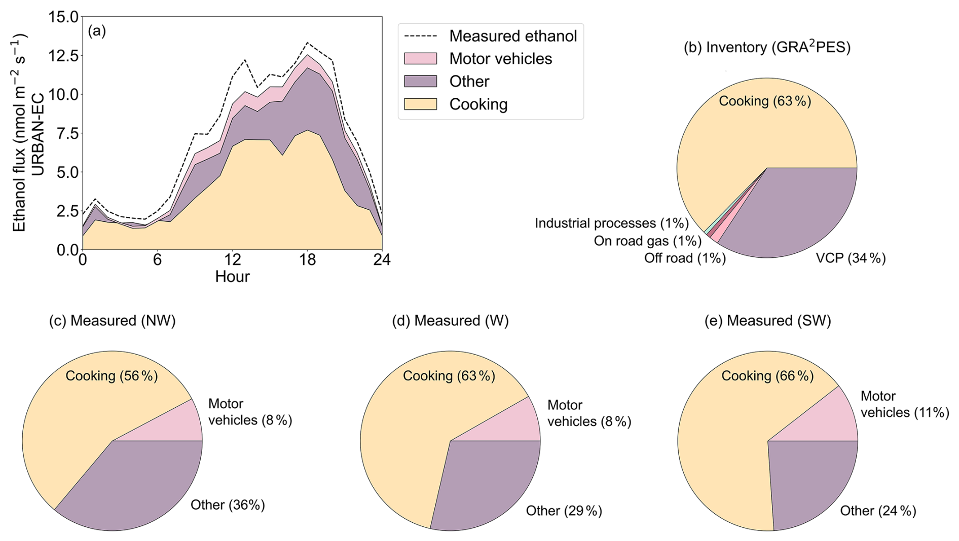
Figure 5 Tracer-based source apportionment results for ethanol and GRA²PES inventory comparison. (a) Median measured flux diurnal profile for each source of ethanol: fossil fuels, other (which includes volatile chemical products, VCPs), and cooking, with the median measured ethanol flux. (b) GRA²PES ethanol source categories. (c–e) Median measured ethanol source apportionment from Northwest (NW), West (W), and Southwest (SW) wind directions. Pie charts include data from daytime hours (07:00–21:00 LT).

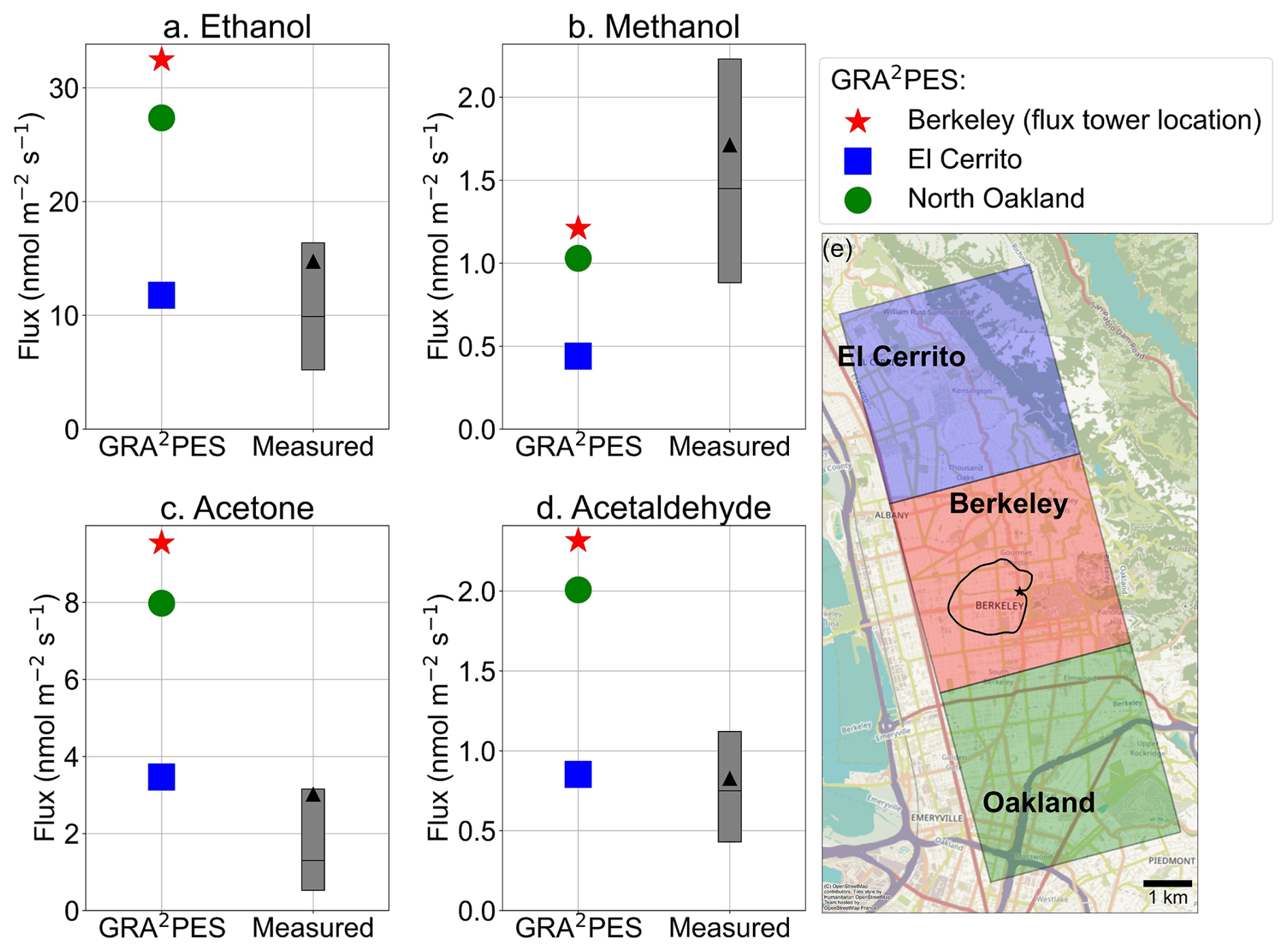
Figure 6 Daytime GRA²PES and measured flux comparison for (a) ethanol, (b) methanol, (c) acetaldehyde, and (d) acetone. GRA²PES grid cells are shown in (e). The flux tower (star icon) is in the Berkeley grid cell. Measured data is the interquartile range (box), median (horizontal line), and mean (triangle icon). The black trace in (e) is the 80 % URBAN-EC flux footprint. For the Berkeley grid cell, the mean daytime ${\mathrm{GRA}}^{\mathrm{2}}\mathrm{PES}/\mathrm{URBAN}$-EC =3.3 (ethanol), 0.8 (methanol), 7.4 (acetone), 3.1 (acetaldehyde). Map data © OpenStreetMap contributors, distributed under the Open Data Commons Open Database License.

3.1.2 Footprint representativeness: Ethanol

The combination of mobile measurements and tower-based flux measurements made in the same geographical area provide a unique opportunity to assess footprint representativeness. While temporally rich, the flux footprint was ∼ 2.8 km² and was therefore limited geographically. Mobile measurements conducted within the footprint and beyond provide additional context on sources of OVOCs in urban areas.

Mobile and tower measurements were not contemporaneous; mobile data collection occurred before the tower was established. Comparing the two datasets assumes that the major OVOC sources sampled were roughly the same between years. Figure S14 compares the range of mixing ratios observed with the mobile laboratory to the flux tower for overlapping months (November, December, January). Generally, there was good agreement between the two datasets for November and December, while tower data from January was lower. On average, mobile laboratory data was 1.1 to 3.6 times higher than tower observations. Since mobile measurements were closer to VOC sources and the sampled airmasses had undergone less dilution, we expected that mobile laboratory mixing ratios would be higher than those measured at the flux tower 40 m above the ground.

Figure 7 shows the median of daily mean ethanol concentrations from mobile monitoring on a 200 m by 200 m square grid with the 80 % flux footprint overlayed. Gridded ethanol concentrations were higher in the southern half of the flux footprint, though measured ethanol fluxes were not significantly different from SW, W, and NW wind directions (p>0.05). Diurnal flux profiles for each wind direction are shown in Fig. S15. Importantly, the highest average ethanol concentrations observed via mobile monitoring were not within the flux footprint, indicating the flux observations could have missed key regional hotspots of ethanol emission (described below in Sect. 3.1.3). The flux footprint included a mixture of commercial and residential zones which are representative of the broader area but did not include industrial zones (Fig. S16). The flux and source apportionment results described above are representative of urban residential and commercial emissions with a strong influence from restaurants but are missing industrial sources.

3.1.3 Sources identified via mobile laboratory: Ethanol

Mobile measurements show that ethanol concentrations increased from West to East across Berkeley and Oakland (Fig. 7). This trend was caused by prevailing westerly winds; emissions accumulated in the air mass as it traveled from West to East. Freeways and industrial activities were concentrated on the Western edges of the mobile sampling domain, and flux observations indicate that motor vehicles were a minor source of ethanol in this location. Low ethanol concentrations were also observed around the Port of Oakland (Southwest Oakland), likely due to limited E10 fuel use in this area and the predominance of diesel and other fossil fuel combustion sources here. The highest ethanol concentrations were observed in Northwest Berkeley, South Berkeley, and North Oakland. Nonanal was not quantified in the mobile laboratory dataset, so cooking emissions could not be assessed here.

The Northwest Berkeley region with high ethanol concentrations includes the city of Berkeley transfer station, industrial zones, breweries, and autobody shops. The transfer station is a major site for waste, compost, and recycle collection, so ethanol emissions from decomposition and solvent evaporation were expected here. Spikes in ethanol concentration covaried with acetone, acetaldehyde, methanol, and other OVOC formulas (e.g., C₄H₉O⁺, C₃H₇O${}_{\mathrm{3}}^{+}$ C₂H₇O${}_{\mathrm{3}}^{+}$) in this area, likely due to solvent use (Fig. 8). The breweries could have also been an important source of ethanol in this region, though close proximity to other ethanol sources made it challenging to attribute ethanol emissions directly to brewing. Areas with high gridded ethanol concentrations in Oakland included a recycling facility, autobody shops, and residential areas. These mobile observations show that waste treatment facilities like transfer stations, composting facilities, and recycling facilities were important sources of ethanol which were not included in the flux footprint. While wastewater treatment facilities are sources of VOCs like methanethiol, the wastewater treatment facility in this domain was not a dominant source of ethanol or other OVOCs included in this analysis.

Spikes in ethanol concentration were correlated with acetone and BTEX (C₆H${}_{\mathrm{6}}^{+}$: benzene, C₇H${}_{\mathrm{9}}^{+}$: toluene, C₈H${}_{\mathrm{11}}^{+}$: ethyl benzene and xylenes) compounds throughout the mobile sampling domain (Fig. 8). Correlations with BTEX were likely from fossil fuel combustion or evaporation, while correlations with acetone were likely from VCP emissions. The predominance of acetone-correlated spikes points towards VCPs as a dominant ethanol source in the region, as opposed to vehicles, consistent with the tracer-based source apportionment results from the flux tower observations.

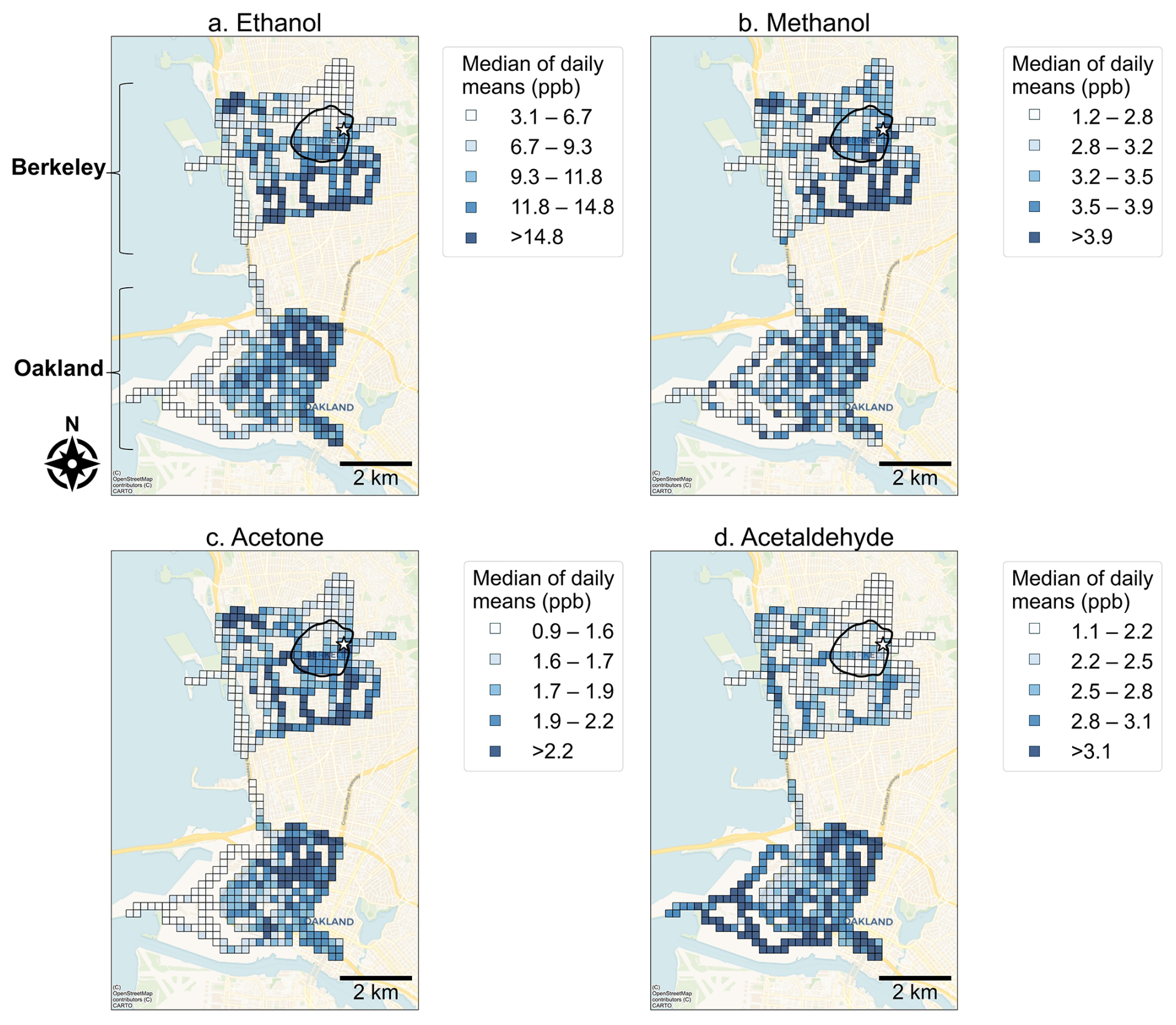
Figure 7 Median of daily mean VOC mixing ratio for each 200 m by 200 m grid cell for (a) ethanol, (b) methanol, (c) acetone, and (d) acetaldehyde. Data are split into quantiles for plotting and grid cell values were capped at the 95th percentile. The black circle represents the 80 % URBAN-EC flux tower footprint, and the star icon is the location of the tower. The northern cluster of grid cells is the Berkeley domain, while the southern cluster of grid cells is the Oakland domain. Map data © OpenStreetMap contributors, distributed under the Open Data Commons Open Database License.

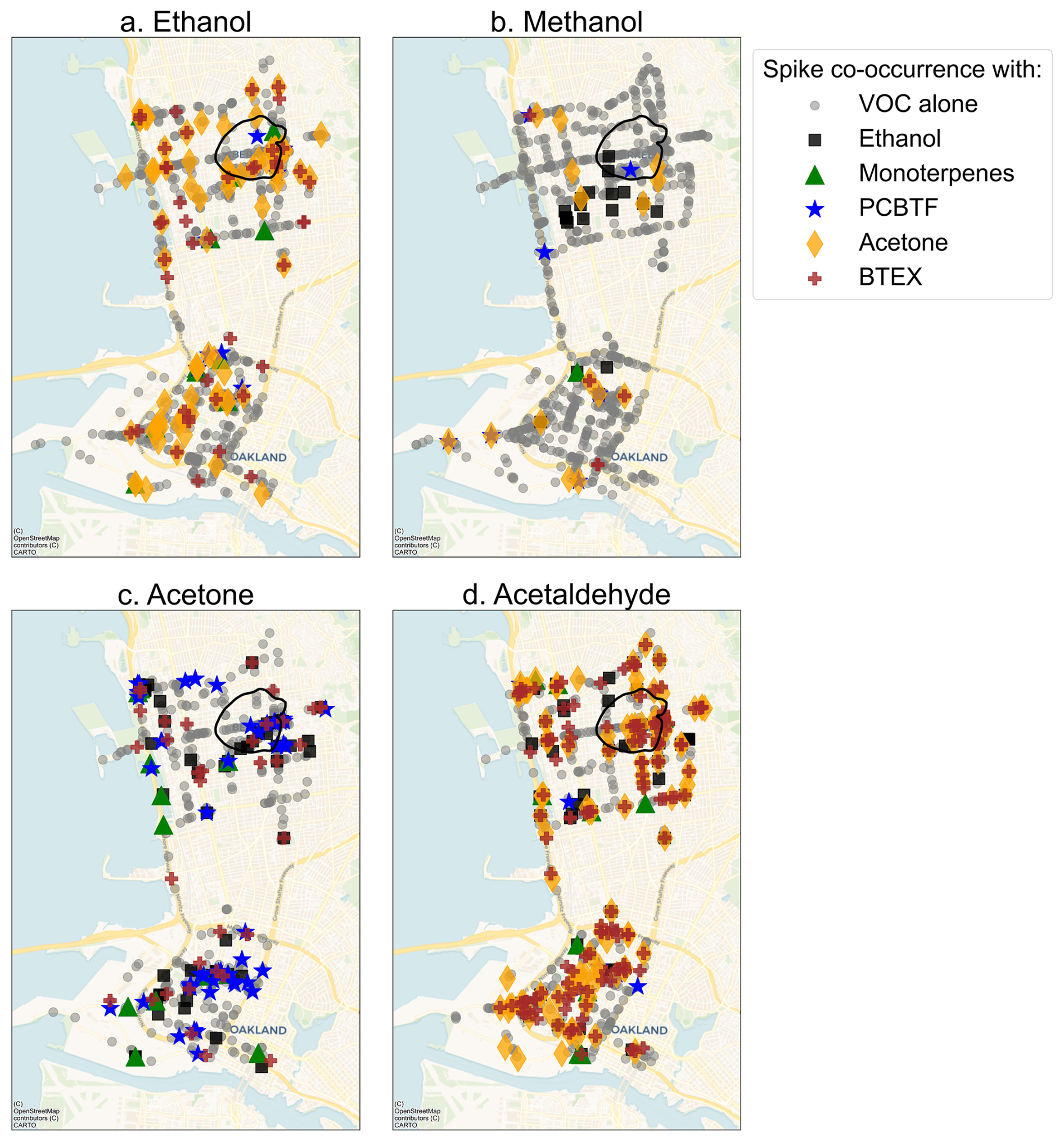
Figure 8 VOC spike colocations for (a) ethanol, (b) methanol, (c) acetone, and (d) acetaldehyde. A VOC spike with no correlations is shown as a grey circle. VOC spike colocation with ethanol: black square, with monoterpenes: green triangle, with parachlorobenzotrifluoride (PCBTF): blue star, with acetone: orange diamond, with benzene, toluene, ethylbenzene, and xylene (BTEX): brown cross. The black circle is the 80 % flux footprint. Map data © OpenStreetMap contributors, distributed under the Open Data Commons Open Database License.

3.2 Methanol (CH₅O⁺)

Methanol was 6 % to 9 % of the median measured molar flux, 1 % of the calculated OH reactivity flux, and 11 % to 17 % of the measured mixing ratio across the seasons. Median methanol fluxes were highest in summer 2022 (1.68 nmol m⁻² s⁻¹) and autumn 2023 (1.76 nmol m⁻² s⁻¹) and lowest in winter 2023–2024 (1.03 nmol m⁻² s⁻¹) (Table 1). Median methanol fluxes in 2022 were highest in June, while median methanol fluxes in 2023 were highest in September (Fig. 3). The weighted average methanol flux was 1.02 ± 0.35 nmol m⁻² s⁻¹ and mixing ratio was 1.12 ±  0.87 ppb (Table 1). Methanol fluxes in Berkeley were consistent with observations from Beijing and Helsinki and lower than observations from London (Table S2). Methanol mixing ratios were similar to observations from Helsinki and about an order of magnitude lower than observations from Beijing and London (Table S3) (Acton et al., 2020; Langford et al., 2010; Rantala et al., 2016). Net deposition was observed for 3.03 % of averaging intervals. Methanol monthly median fluxes were correlated with ethanol (R²=0.70), indicating similar long-term variability, however, the high frequency (30 min) correlation was low (R²=0.05), suggesting that this relationship does not arise from coupled short-term emission events. Biogenic methanol emissions are important globally, but they were minimal in the flux footprint relative to anthropogenic sources. Methanol emissions from MEGAN were about an order of magnitude lower than observations during June to October 2022 (Fig. S11).

VCPs are a major source of anthropogenic methanol. GRA²PES indicates that all the methanol emissions in the flux tower grid cell were from VCPs (Fig. S17). The magnitude and diurnal profile of methanol emission in GRA²PES agrees well with observations (Figs. 7, S17). Methanol was the only OVOC analyzed here that had lower emissions in GRA²PES relative to median observations for the local grid cell. (average daytime ${\mathrm{GRA}}^{\mathrm{2}}\mathrm{PES}/\mathrm{URBAN}$-EC ratio = 0.8). Methanol emissions have been reported during indoor cooking (Arata et al., 2021; Kumar et al., 2025), however, this source is absent from the inventory.

Methanol mixing ratios measured via mobile monitoring were highest outside of the flux footprint, indicating important methanol sources may be absent from the flux tower observations (Fig. 7). Like ethanol, methanol mixing ratios increased from West to East, and the lowest methanol mixing ratios were observed on the Western edge of the mobile sampling domain. Methanol emissions from on-road sources were not expected. The highest methanol mixing ratios were observed in predominantly residential neighborhoods in Oakland and South Berkeley, consistent with indoor to outdoor emissions. Spikes in methanol concentration typically did not correlate with other VOCs (Fig. 8). A small fraction of methanol spikes was correlated with ethanol and acetone, consistent with a VCP source.

Indoor to outdoor transport of methanol could be an important source of methanol in urban environments due to its high concentration indoors (Nazaroff and Weschler, 2024). Arata et al. (2026) estimated that 13 % to 26 % of outdoor methanol is of indoor origin in the same region as this study. Using the weighted average methanol flux and footprint population density, the emission factor is ∼ 450 mg d⁻¹ per person, while Nazaroff and Weschler (2024) estimated that methanol emissions from indoor to outdoor transport are 96 mg d⁻¹ per person. By comparing these two emission factors, we find that ∼ 21 % of the measured methanol flux could be of indoor origin, which agrees well with the estimate from Arata et al. (2026).

3.3 Acetone (C₃H₇O⁺)

3.3.1 Flux tower observations: Acetone

Acetone was 6 % to 9 % of the median measured molar flux, < 1 % of the calculated OH reactivity flux, and 9 to 13 % of the measured mixing ratio across the seasons. Median acetone fluxes were the highest in summer 2023 (1.81 nmol m⁻² s⁻¹) and lowest in winter 2023–2024 (1.01 nmol m⁻² s⁻¹) (Table 1). The weighted average acetone flux was 1.68 ± 1.25 nmol m⁻² s⁻¹ and mixing ratio was 0.80 ± 0.42 ppb (Table 1). Acetone fluxes in Berkeley were similar to fluxes measured in summer and autumn in Beijing and London but were higher than observations from Helsinki (Table S2). Acetone mixing ratios in Berkeley were consistent with other studies (Table S3) (Acton et al., 2020; Langford et al., 2010; Rantala et al., 2016).

Substantial interannual variability of acetone flux was observed for June and July, and these differences were most likely caused by episodic anthropogenic sources. The interquartile range of acetone fluxes in June and July 2023 was wider than corresponding months in 2022; the 75th percentile, mean, and median were higher in 2023. Acetone fluxes were relatively constant from June through October in 2022. There was construction activity in the flux footprint throughout the two years of sampling, which was likely a source of the interannual variability of acetone emissions, presumably through VCP use. Day of week variability also suggests construction was a key source of acetone. Daytime acetone fluxes were significantly lower on Sundays than every other day of the week (p<0.05, significance was tested for each day individually). On average, daytime fluxes of acetone were 121 % higher Monday through Saturday relative to Sunday. This pattern indicates there were anthropogenic sources of acetone, such as construction, Monday through Saturday that were absent or lower on Sundays. Figure S18 shows the median diurnal flux of acetone for each day of the week; the trend for Sunday was distinct from all other days. This day of week variability was not captured by GRA²PES; emissions were less than 0.15 % different on weekdays relative to Saturdays and Sundays.

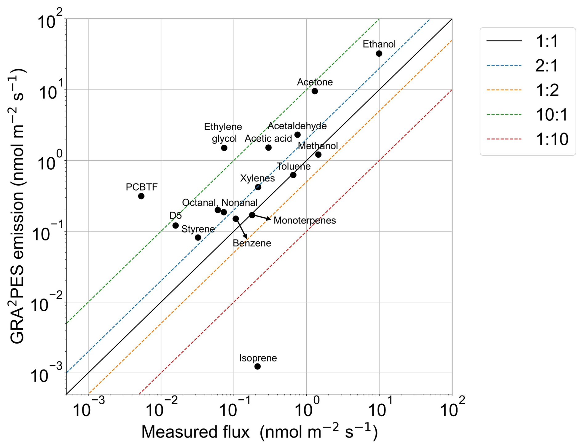
Figure 9 Scatter plot of median daytime GRA²PES emission (2023 August weekday) versus the median daytime measured flux on a Log versus Log plot. The 1:1, 2:1, and 10:1 lines are shown. GRA²PES emissions represent anthropogenic VOC sources.

80 % of acetone emissions in GRA²PES were attributed to VCPs and 18 % were attributed to cooking (Fig. S17). Both Acetone and PCBTF were over-estimated in GRA²PES by about an order of magnitude or more (Fig. 9). Sporadic, high emissions of these VOCs, which originate predominantly from VCPs, are challenging to quantify using bottom-up methods. BTEX compounds had better agreement with observations, consistent with prior studies (e.g., Pfannerstill et al., 2023) (Fig. 9). This comparison shows that GRA²PES was more accurate for vehicle emissions, while VCP and cooking emissions were over-estimated. These discrepancies are consistent with motor vehicle emissions having been studied extensively for decades, while VOC emissions from VCPs and cooking have only recently become key research interests.

3.3.2 Mobile laboratory observations and footprint representativeness: Acetone

Like ethanol, acetone concentrations increased from West to East across Oakland and Berkeley as emissions accumulated in the air mass (Fig. 7). Acetone concentrations were elevated in the Northwest region of Berkeley near the trash transfer station, recycling center, and autobody shops. High acetone concentrations were also observed in the Southeast part of the flux footprint and in residential neighborhoods of Oakland. The distribution of acetone concentrations observed with the mobile laboratory indicates the flux footprint included some regions with high acetone emissions, but it was still missing key industrial sources.

Spikes in acetone concentration were frequently correlated with parachlorobenzotrifluoride (PCBTF), a tracer for solvent emissions, and BTEX (Fig. 8). Acetone and PCBTF spike correlations were not observed with BTEX spikes, indicating at least two distinct solvent-based acetone sources were sampled: one that includes PCBTF and one that includes BTEX. Benzene is not an ingredient in solvents in California, so acetone correlations with BTEX could indicate that VCP sources were near on-road sources or that C₆H${}_{\mathrm{7}}^{+}$, the ion used for benzene detection in the mobile dataset, was influenced by fragmentation of substituted aromatics. 37 acetone spikes were correlated with PCBTF where the PCBTF/acetone ratio ranged from 0.01 to 2.45. The wide range of ratios indicates there are a wide range of solvent formulations for different applications with unique PCBTF/acetone ratios. There were at least three major regions in the mobile sampling domain where spikes of acetone and PCBTF correlated, one of which was included in the flux footprint. However, correlations were not observed between PCBTF and acetone in the flux tower data.

3.4 Acetaldehyde (C₂H₅O⁺)

3.4.1 Flux tower observations: Acetaldehyde

Acetaldehyde was 3 % to 4 % of the median measured molar flux, 6 % to 7 % of the calculated OH reactivity flux, and 5 % to 8 % of the measured mixing ratio across the seasons. Median acetaldehyde fluxes were highest in summer (0.95 and 0.82 nmol m⁻² s⁻¹) and lowest in winter (0.29 nmol m⁻² s⁻¹). The campaign weighted average flux of acetaldehyde was 0.47 ± 0.21 nmol m⁻² s⁻¹. Acetaldehyde fluxes measured in the summer were higher than observations from Helsinki and lower than observations from Beijing and London (Table S2). The seasonal trend of acetaldehyde flux was generally consistent between 2022 and 2023 (Fig. 3); the highest fluxes were observed from June to September. Like ethanol and methanol, acetaldehyde fluxes were higher in June 2022 than June 2023. Acetaldehyde mixing ratios were highest in October, November, and December, and lowest in May through August (Fig. S7). Mixing ratios were lower in 2022 than in 2023. Like the other OVOCs, trends in acetaldehyde mixing ratio were generally caused by boundary layer dynamics as opposed to direct emissions. Photochemical production was also likely a key driver of mixing ratio trends. The campaign weighted average mixing ratio of acetaldehyde was 0.52 ± 0.31 ppb. Acetaldehyde mixing ratios were consistent with observations from Helsinki and lower than Beijing and London (Table S3) (Acton et al., 2020; Langford et al., 2010; Rantala et al., 2016).

Like ethanol, we estimated the source apportionment of acetaldehyde using a tracer-based approach. Acetaldehyde is emitted during cooking through the thermal degradation of cooking oils and other chemical processes (e.g., the Maillard reaction). The GRA²PES inventory indicates cooking was the dominant anthropogenic source of acetaldehyde in the local grid cell and that on road sources and industrial processes were minor contributors to acetaldehyde emission (Fig. S17). The emissions inventory was 3.1 times higher than median measured acetaldehyde fluxes in our grid cell, suggesting the magnitude of acetaldehyde emissions from cooking were lower than what was prescribed in GRA²PES. Acetaldehyde was also an important contributor to the measured VOC emission during indoor cooking experiments (Arata et al., 2021). We determined the flux of acetaldehyde from cooking (F_AcAl,cooking, Eq. 5) by multiplying F_EtOH,cooking (Eq. 3) by the acetaldehyde/ethanol ratio from the cooking experiments reported by Arata et al. (2021) ($R_{\mathrm{AcAl}/\mathrm{EtOH},\mathrm{cooking}}=\mathrm{0}$.06). To evaluate the uncertainty in this estimate, we performed a bootstrap analysis where observations were sampled with replacement 10 000 times. For each sample, we performed Monte Carlo sampling of $R_{\mathrm{AcAl}/\mathrm{EtOH},\mathrm{cooking}}$ by randomly varying $R_{\mathrm{AcAl}/\mathrm{EtOH},\mathrm{cooking}}$ within its plausible range (Fig. S19). The plausible values were selected from a triangular distribution with a mode of 0.06 between 0.03 (lowest ratio from the literature) and 0.07 (highest plausible value for our study). The range of $R_{\mathrm{AcAl}/\mathrm{EtOH}}$ for cooking in the literature spans three orders of magnitude (0.03 to 1.33) (Arata et al., 2021; Coggon et al., 2024a; Kumar et al., 2025). However, using $R_{\mathrm{AcAl}/\mathrm{EtOH},\mathrm{cooking}}$ above 0.08 in the tracer-based source apportionment approach caused the total calculated acetaldehyde flux to be higher than the measured acetaldehyde flux, indicating a lower ratio is more representative of the integrated cooking emissions sampled during this study. Through this method, 42 % (median value, 95 % CI = 27 %–52 %) of the acetaldehyde flux was attributed to cooking (Fig. S19). The fraction of acetaldehyde attributed to cooking was higher in 2023 than 2022, which may be caused by higher restaurant emissions, as meteorological drivers were not different.

$$\begin{array}{}\text{(5)}& F_{\mathrm{AcAl},\mathrm{cooking}}=R_{\mathrm{AcAl}/\mathrm{EtOH},\mathrm{cooking}}\cdot F_{\mathrm{EtOH},\mathrm{cooking}}\end{array}$$

Combustion is also an important source of acetaldehyde in urban areas. The GRA²PES inventory reports acetaldehyde emissions from on-road and off-road source categories. We determined the acetaldehyde flux from fossil fuel combustion sources (F_{AcAl,FFcombustion}) by multiplying F_benzene by the average acetaldehyde/benzene ratio from on road (1.34) and off-road source (1.52) categories in GRA²PES ($S_{\mathrm{AcAl},\mathrm{FFcombusion}}=\mathrm{1}$.43). Through this method, 23 % (campaign median) of the measured acetaldehyde flux was from on road and off-road combustion sources.

$$\begin{array}{}\text{(6)}& F_{\mathrm{AcAl},\mathrm{FFcombustion}}=S_{\mathrm{AcAl},\mathrm{FFcombusion}}\cdot F_{\mathrm{benzene}}\end{array}$$

The measured acetaldehyde flux less the sum of F_AcAl,cooking and F_{AcAl,FFcombustion} (F_AcAl,other) is attributed to other miscellaneous or unknown sources, including photochemical production. Median monthly acetaldehyde fluxes were correlated with median PPFD (R²=0.72), suggesting that photochemical production of acetaldehyde was an important source in the footprint. The correlation with temperature was lower (R²=0.22). The largest source of acetaldehyde globally is photochemical production, where alkanes, alkenes, and ethanol are the main precursors (Millet et al., 2010). Transport time from emission to measurement at the URBAN-EC tower is ∼ 100 s, which is too short for photochemical production of acetaldehyde from VOC precursors to drive the observed acetaldehyde fluxes. Instead, photochemical or thermal degradation of materials at the surface or heterogeneous aerosol chemistry could be sources of acetaldehyde. Photodegradation of polymeric esters including polyvinyl acetate (PVAC) produced acetaldehyde under vacuum ultraviolet exposure (Buchanan and McGill, 1980). While the radiation intensity would be different at Earth's surface, some polymer degradation is expected. The fraction of F_AcAl,other was lowest in the winter, consistent with decreased photochemical production (Fig. 10). Median acetaldehyde fluxes were also correlated with RH in 2023–2024 (R²=0.81). F_AcAl,other may also include indoor to outdoor transport, as acetaldehyde is an important VOC in indoor environments (Salthammer, 2023).

$$\begin{array}{}\text{(7)}& F_{\mathrm{AcAl},\mathrm{other}}=F_{\mathrm{AcAl}}-F_{\mathrm{AcAl},\mathrm{combusion}}-F_{\mathrm{AcAl},\mathrm{cooking}}\end{array}$$

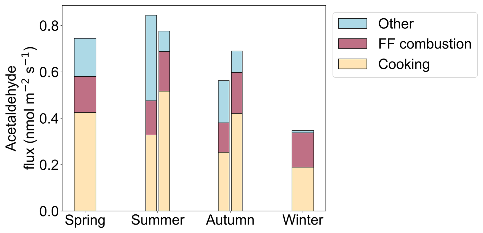
Figure 10 Median acetaldehyde flux for each season. For summer and autumn, the left bar is 2022, and the right bar is 2023. The flux is separated using the tracer-based source apportionment approach into cooking, fossil fuel (FF) combustion, and other sources.

3.4.2 Mobile laboratory observations and footprint representativeness: Acetaldehyde

Gridded concentrations of acetaldehyde were lower in Berkeley than in Oakland (Fig. 7), indicating the flux tower observations may be biased low relative to surrounding neighborhoods. The Port of Oakland and freeways were likely important sources of acetaldehyde in Oakland that were not present in the flux footprint. Diesel truck traffic is high in these areas and could represent a key acetaldehyde source (Song et al., 2010). In West Berkeley, slightly elevated concentrations of acetaldehyde were observed, also likely due to the freeway. The lowest concentrations of acetaldehyde in the entire mobile sampling domain were in the flux footprint.

Spikes in acetaldehyde concentration were frequently correlated with BTEX (18 % of the observed acetaldehyde spikes) (Fig. 8). Individual components of BTEX (e.g., benzene, toluene) were correlated with 20 %–22 % of acetaldehyde spikes. 17 % of acetaldehyde spikes were correlated with C₇H₉O⁺, an ion formula consistent with cresols, which can originate from automobile exhaust. These correlations with vehicle tracers highlight the importance of on-road sources for acetaldehyde in the broader East Bay Area, a minor source in the URBAN-EC footprint.

4 Conclusions

We combined volatile organic compound (VOC) fluxes from a long-term urban tower deployment, URBAN-EC, with mobile measurements of the same key species within the flux footprint and beyond to assess prominent urban VOC sources. Oxygenated VOCs (OVOCs) comprised a substantial fraction of the measured VOC molar flux (70 %), mixing ratio (69 %), and calculated OH reactivity flux (27 %). Ethanol had the highest median mixing ratio and flux of all the measured VOCs, while methanol, acetone, and acetaldehyde were also key contributors. Cooking and volatile chemical products (VCPs) were the main sources of these OVOCs, highlighting the importance of non-traditional VOC sources (i.e., not related to on-road combustion sources) in densely populated urban areas. These results also corroborate recent evidence that indoor environments are important VOC sources in urban environments (Arata et al., 2026; Zhou et al., 2025).

These long-term, continuous measurements provide a unique perspective on the seasonal and diel cycles of urban OVOC emissions and mixing ratios. At this location, late autumn and winter had the highest OVOC mixing ratios, while OVOC fluxes were generally lowest in the winter. Most OVOC mixing ratios followed a similar median trend throughout the year, driven by meteorology, while OVOC fluxes had distinct seasonal trends, indicating they had unique sources within the flux footprint. Lower winter fluxes were likely caused by lower local emissions (e.g., lower indoor-to-outdoor emissions). These directly calculated fluxes are useful for source apportionment and serve as benchmarks for VOC emissions inventory validation and development.

Ethanol was about half of the measured flux and ∼20 % of the calculated OH reactivity flux and was therefore a central component of the urban VOC emissions. We utilized a tracer-based source apportionment approach to quantify ethanol fluxes from relevant sources. Cooking was the predominant source of ethanol; 56 % to 66 % of the measured ethanol flux was attributed to cooking, depending on wind direction. VCP emissions, indoor-to-outdoor transport, and other sources were responsible for 24 % to 36 % of the measured ethanol flux, and on-road sources contributed ∼10 % of the measured ethanol flux. Prior studies have also shown that cooking is a key driver of urban VOC emissions and ozone formation (Stockwell et al., 2025; Zhu et al., 2025).

By analyzing mobile and flux measurements from the same geographic area, we were able to determine the representativeness of the flux measurements, which were limited spatially, in the broader urban area. The flux tower results were generally representative of urban residential and commercial zones but likely missed some industrial and on-road emissions. Mobile monitoring results showed that industrial zones and waste treatment facilities were important sources of ethanol, acetone, and methanol emissions, and fossil fuel combustion was an important source of acetaldehyde. Future studies may use mobile monitoring to inform eddy covariance site placement or quantify the flux of OVOCs from specific sources, such as waste treatment facilities. This work demonstrates the importance of combining multiple methodologies.

The geographic distribution of OVOC mixing ratios showed that steep spatial gradients were present in this urban area. The OVOCs analyzed here, except for acetaldehyde, increased in concentration from West to East across the sampling domain due to predominantly westerly winds and because the freeways and port on the Western sampling edge were not major sources of ethanol, methanol, and acetone. Comparing the spatial distribution of mixing ratios for ethanol, methanol, and acetone revealed three key shared hotspots: (1) Northwest Berkeley, (2) Northeast Oakland, and (3) South Berkeley. Hotspots 2 and 3 are predominantly residential neighborhoods, while Hotspot 1 is an industrial area with waste treatment facilities. The spatial distribution of acetaldehyde was not like these other OVOCs, indicating disparate sources. Acetaldehyde mixing ratios were higher in the Oakland sampling domain, and local mixing ratios were highest around freeways and the port, consistent with a fossil fuel combustion source.

This work advances current understanding of urban VOC sources and improves predictive capabilities in air quality models. We compared the directly measured VOC fluxes to GRA²PES, a state-of-the-art emissions inventory. This detailed evaluation has both validated and identified knowledge gaps in our understanding of urban VOC sources. GRA²PES roughly agreed with the tracer-based source apportionment for ethanol (i.e., cooking was a dominant source of ethanol), but the total emission was a factor of ∼ 3 to 4 times higher in magnitude than observations. These comparisons support that cooking is an important VOC source in urban areas, especially in areas with a high density of restaurants. The previous version of this inventory prior to 2025, FIVE-VCP, did not include cooking. GRA²PES was 3 and 7 times higher than observations for acetaldehyde and acetone, respectively, and 0.8 times lower than observations for methanol. These results contrast prior eddy covariance measurements in urban areas of Southern California, which showed that OVOC emissions in FIVE-VCP were lower than observations, as opposed to higher (Pfannerstill et al., 2023). The addition of cooking in the GRA²PES inventory improved source apportionment comparisons but overestimated the total emissions magnitude for many OVOCs. The inventory/measurement comparison was generally more accurate for the northern neighboring grid cell with lower population density compared to the grid cell containing the flux tower, indicating potential issues with population density scaling for this region. Future work evaluating emissions inventories should consider multiple regions with diverse population and restaurant densities to understand how population scaling impacts the comparisons.

In the future, more source-specific studies of major urban VOC emission sources like restaurants and waste treatment facilities will continue to advance representation of VOCs in models. Additionally, eddy covariance flux measurements in more urban areas, both through stationary towers and aircraft-based deployment, will help constrain uncertainties in emission inventories.