Aerosol vertical distributions shaped by boundary layer dynamics in a coastal urban environment: insights from the TRACER campaign

Aerosol vertical distributions are a major source of uncertainty in quantifying aerosol–cloud–climate interactions. Using observations collected during the 2022 TRACER campaign in Houston, Texas, we investigate how atmospheric boundary layer dynamics shape the vertical structure of aerosol populations in a coastal urban environment. Our lidar retrieval combines micropulse lidar backscatter with ground-based aerosol measurements to obtain aerosol concentration profiles. A compact framework for describing aerosol vertical profile shape is needed to examine factors that influence aerosol vertical distributions and to represent them in model parameterizations or remote sensing retrievals. We introduce a parameterized fitting function for characteristic S-shaped aerosol profiles, with fitted parameters that represent aerosol-layer depth and stratification strength. This parameterization is applied to case studies demonstrating how boundary-layer dynamics, including turbulent mixing, capping inversion strength, and sea-breeze circulations, influence aerosol vertical distributions. Case studies show that aerosol concentrations decrease rapidly near strong capping inversions, the depth of the lower aerosol layer changes with boundary-layer growth and collapse, and sea-breeze passage produces strong coastal–inland differences as maritime air replaces continental aerosol. Analysis of the six-month dataset shows weak but statistically significant positive relationships between daytime boundary layer height and fitted aerosol layer depth, and between the local potential temperature gradient near the aerosol layer top and fitted stratification strength parameter. Finally, we demonstrate an approach for estimating aerosol profile shape from boundary-layer height and potential-temperature gradients using the fitted parameterization. These results show that this parameterization provides simple, interpretable diagnostics for linking aerosol profile shape to boundary-layer dynamics.

1 Introduction

Aerosols play a crucial role in influencing Earth's climate directly through interactions with solar radiation and indirectly through aerosol–cloud interactions (Haywood and Boucher, 2000; Kahn, 2012; Seinfeld et al., 2016). Aerosols scatter and absorb short and longwave radiation, thus contributing to direct aerosol radiative forcing (Szopa et al., 2023). Aerosols can also act as cloud condensation nuclei (CCN) and ice nucleating particles (INPs) to facilitate cloud formation, which leads to the aerosol indirect radiative effect (Twomey, 1977; Albrecht, 1989; Kanji et al., 2017; Burrows et al., 2022). In addition, light absorbing aerosols can heat the surrounding air, affect thermodynamic stability and cloud formation, and lead to the aerosol semi-direct radiative effect (Johnson et al., 2004). Therefore, to better quantify the radiative effects of aerosols, it is important to accurately characterize the spatial and temporal variations in aerosol concentration, size distributions, and physicochemical properties. Among these factors, aerosol vertical distributions significantly influence both the direct and indirect radiative effects. In the presence of clouds, whether aerosols are located above or below the cloud substantially affects their direct radiative forcing (Choi and Chung, 2014). Under cloud-free conditions, the direct radiative effect of aerosols depends on the height of the aerosol layers (Mishra et al., 2015). Further, the magnitude of the aerosol direct radiative effect tends to increase with aerosol layer height in the ultraviolet and thermal infrared regions but decreases with aerosol layer height in the visible to near infrared range (Mishra et al., 2015). Simulations show that the altitude of aerosols critically influences how they are mixed in developing clouds, alter microphysical processes, and ultimately impact the strength of updrafts, cold pools, and resulting precipitation in deep convective systems (Lebo, 2014; Marinescu et al., 2017; Zhang et al., 2021). Long term observations demonstrate how different patterns of aerosol vertical distributions influence warm cloud properties, with aerosols suppressing cloud water production in continental environments but enhancing it in marine environments (Lin et al., 2023). Therefore, improving our understanding of the aerosol vertical distributions is one of the key challenges in reducing uncertainties in aerosol–cloud–climate interactions, refining climate models, and advancing our ability to predict future climate scenarios (Johnson et al., 2004; Kahn, 2012; Fan et al., 2016; Lin et al., 2023).

Both in situ and remote sensing observations have been used to examine aerosol vertical distributions, revealing complex spatial and temporal variability in aerosol characteristics. In situ aircraft measurements provide direct observations of aerosol concentration, size distribution, and chemical composition. Large concentrations of accumulation mode aerosols have been observed in the boundary layer, particularly in the northern extratropics due to anthropogenic emissions (Watson-Parris et al., 2019). Above the boundary layer top, new particle formation leads to a shift toward smaller particle sizes with increasing altitude (Watson-Parris et al., 2019). In clean marine regions, aerosol concentration can increase with altitude due to the homogeneous nucleation of small volatile particles at higher altitudes, while sea salt aerosols dominate at lower altitudes (Clarke and Kapustin, 2010). In more polluted marine regions, long range transport contributes to increased aerosol concentration above 4 km (Clarke and Kapustin, 2010). Over continental regions, emissions from urban and industrial sources result in large aerosol concentrations near the surface (Clarke and Kapustin, 2010). Analysis of aircraft measurements reveals that the thermodynamic stability of the atmospheric boundary layer has a significant influence on the shape of the aerosol vertical profile. When stable layers, such as nocturnal or frontal inversions, are present, vertical mixing is suppressed, trapping aerosols within the boundary layer and creating a sharp concentration gradient above it (Zhang et al., 2009).

Modeling studies also provide some insight on the factors that may control aerosol vertical distributions (Freire et al., 2016; Nissanka et al., 2018; Xiao and Taylor, 2002). The atmospheric boundary layer dynamics and processes also play a central role in shaping aerosol vertical profiles. The distribution of aerosols within the boundary layer is controlled by the balance between vertical turbulent transport and gravitational settling. When these processes are in equilibrium, the surface layer aerosol concentrations generally follow a power law relationship (Hoppel et al., 2002; Xiao and Taylor, 2002). Larger particles experience stronger gravitational settling, leading to a steeper concentration decline with height, while smaller particles are more influenced by turbulent mixing, resulting in a more gradual decrease and a more uniform vertical distribution. Under unstable conditions, strong turbulent mixing distributes aerosols more evenly throughout the boundary layer, while in stable conditions, weak turbulence keeps aerosols concentrated near the surface (Freire et al., 2016; Nissanka et al., 2018). Since boundary layer mixing influences the vertical distributions of surface emitted aerosols like sea salt and mineral dust (Kipling et al., 2016), boundary layer evolution throughout the day may lead to corresponding diurnal changes in aerosol profiles (Zhang et al., 2023; Haman et al., 2012).

Simplified representations of aerosol vertical distributions have been used to support remote sensing retrievals of aerosol and trace-gas properties (Wu et al., 2017; Nelson and O'dell, 2019) and to estimate surface aerosol extinction from column observations (Su et al., 2017; He et al., 2016). Similar representations have also been used to prescribe and parameterize aerosol distributions in numerical models for radiative transfer calculations (Ruiz-Arias et al., 2014) and simulations of atmospheric chemistry and cloud processes (Zhao et al., 2021; Stevens et al., 2017). These representations use Gaussian function (Wu et al., 2017; Nelson and O'dell, 2019), exponentially decreasing profile (Ruiz-Arias et al., 2014; Zhao et al., 2021), beta-function (Stevens et al., 2017) and piece-wise profile shape with uniform distribution within the boundary layer (Zhao et al., 2021; He et al., 2016). However, the complexity and variability of aerosol vertical structure can be difficult to capture with simple aerosol profile parameterization (Reid et al., 2017). For example, profiles examined in this study combine a steep near-surface decrease, a relatively uniform layer above, and a sharp transition to cleaner air aloft (Fig. 2c). This vertical structure is difficult to represent with a single exponential or Gaussian function.

Despite the level of vertical detail they provide, aircraft in situ observations are limited in temporal and spatial coverage. Surface measurements can offer routine and continuous observations but cannot capture vertical information. Lidar measurements allow routine aerosol vertical profile measurement, yet optical measurements are strongly affected by aerosol hygroscopic growth. More comprehensive analysis methods integrating both in situ observations and remote sensing techniques are needed to improve our understanding of the factors governing aerosol vertical distributions. This knowledge can be further used to predict aerosol vertical profiles when airborne and lidar measurements are not available and to provide more realistic aerosol data for aerosol–cloud interaction studies. During the 2022 TRacking Aerosol Convection interactions ExpeRiment (TRACER) field campaign, a suite of comprehensive atmospheric data, including thermodynamic profiles, ground-based lidar observations, and surface aerosol measurements, was collected across multiple sites in the Greater Houston, Texas area (Rapp et al., 2024; Jensen et al., 2025). Using our newly developed method by combining ground-based aerosol and lidar measurements, we retrieve aerosol vertical profiles informed by micropulse lidar backscatter coefficient corrected for relative humidity dependent hygroscopic growth, combined with surface measurements of aerosol, CCN, and INPs (Chen et al., 2025).

In this study, we combine aerosol profiles derived from lidar with meteorological observations to characterize typical aerosol vertical distributions in a coastal urban environment and to quantify how boundary layer height (BLH) and stability together control the shape of these profiles. We also provide a set of fitting functions that streamline aerosol vertical profile parameterization, facilitate the incorporation of aerosol vertical profiles into cloud-resolving models, and provide insights into understanding the physical processes governing aerosol vertical distributions. A further goal is to assess the extent to which aerosol vertical profiles can be predicted using only routine meteorological observations and surface aerosol measurements, in the absence of lidar observations.

2 Method

2.1 Field campaign and data collection

Our analysis focuses on data from the TRACER campaign, organized by the U.S. Department of Energy, from October 2021 through September 2022. The primary measurements were made in the Greater Houston Area, Texas. Throughout the campaign, the ARM Mobile Facility (AMF-1) operated continuously at La Porte, Texas shown in Fig. 1 (Jensen et al., 2025). Additional aerosol and meteorological data were collected by deploying Texas A&M University's Rapid Onsite Atmospheric Measurement Van (ROAM-V) alongside radiosonde launches at multiple locations spanning coastal and inland environments (Fig. 1) on selected days when isolated convection was expected (Rapp et al., 2024; Thompson et al., 2025a, b; Lei et al., 2025). As shown in Fig. 1, the coastal site is in Galveston, Texas, while the inland sites include locations in Hempstead and Hockley, Texas.

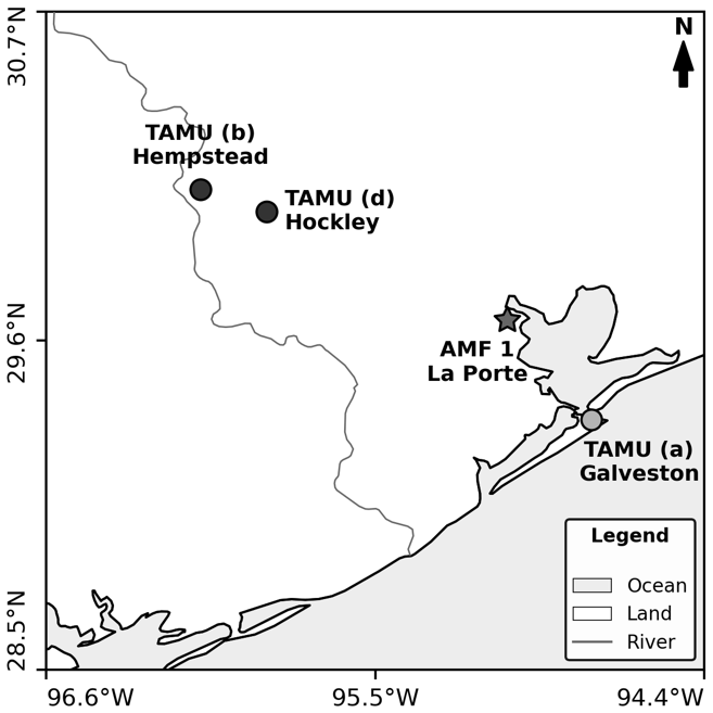
Figure 1 TRACER campaign sampling locations in the Houston, Texas, metropolitan area. The Texas A&M University sampling sites are marked with circles, the ARM AMF1 site is marked with a star. The map is reproduced from Fig. 1 of Chen et al. (2025).

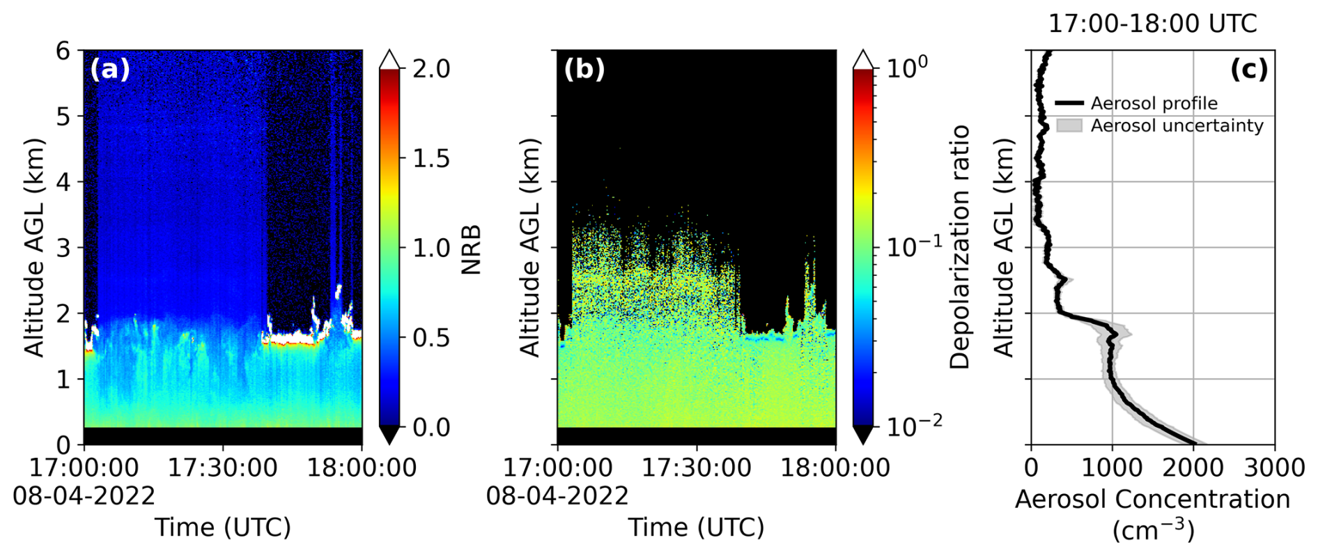
Figure 2 Micropulse lidar measurements on 4 August 2022, at AMF-1 site (a) normalized relative backscatter time-height plot (b) linear depolarization ratio time-height plot (c) retrieved aerosol concentration vertical profile.

2.2 Aerosol vertical profile retrieval using the micropulse lidar

In this work, we employ a method to integrate micropulse lidar and ground-based aerosol measurements to retrieve aerosol vertical distributions corrected for aerosol hygroscopic growth (Chen et al., 2025). Interested readers are referred to Chen et al. (2025) for methodological details. In brief, the procedure first applies an inversion to lidar measurements of attenuated backscatter to obtain an hourly time-averaged cloud-free aerosol backscatter coefficient profile. Next, we use the aerosol hygroscopicity parameter κ, along with Mie scattering theory, to account for aerosol hygroscopic growth at increased humidity measured by the radiosonde, allowing us to convert the retrieved ambient backscatter coefficient to its dry equivalent. The aerosol hygroscopicity parameter κ used for AMF-1 retrieval was estimated from Aerosol Chemical Speciation Monitor (ACSM) aerosol composition measurements collected during the TRACER campaign, with κ values provided by Maria A. Zawadowicz (personal communication, 2025), and are shown in Fig. S1 in the Supplement. The κ values used for TAMU retrieval were estimated from CCN concentration and aerosol size distribution (Chen et al., 2025). This step is crucial because lidar measures optical signals affected by aerosol hygroscopic growth. As aerosols take up water, they grow in size, scatter more light, and increase the lidar backscatter signal without increasing aerosol concentration. Correcting for the aerosol hygroscopic growth effect prevents overestimation of aerosol concentration at altitudes with higher relative humidity. Finally, we calculate the surface aerosol number concentration by integrating the measured aerosol number size distribution and scale this concentration vertically by the ratio of the dry backscatter at each altitude to that near the surface. No standard temperature and pressure (STP) normalization is applied, and all aerosol number concentrations are reported per unit ambient air volume at each altitude. This scaling assumes that the surface aerosol number size distribution is representative aloft. Houston aircraft measurements show that aerosol concentrations and size distributions differ among urban and industrial plumes (Brock et al., 2003; Lance et al., 2009). Such vertical variability cannot be resolved by the single wavelength lidar and remains a source of uncertainty in the retrieved aerosol concentration profiles.

Following Chen et al. (2025), uncertainty in the retrieved aerosol concentration profile was estimated by repeating lidar retrieval and humidity correction with different aerosol lidar ratios, calibration scattering ratios, κ values, and aerosol refractive indices. A geometric standard deviation of 1.5 was used to define the κ sensitivity range by multiplying and dividing the central κ value by 1.5. Temporal variability in the surface aerosol concentration was included using the relative standard error of the mean (SEM) calculated from the condensation particle counter measurements during each retrieval period. This relative SEM was applied to the surface aerosol concentration and propagated into the profile uncertainty. The range of resulting profiles was taken as the uncertainty. This range reflects only the retrieval parameters and surface-concentration variability considered here and should not be interpreted as a complete confidence interval or as indicating high confidence in the retrieved aerosol concentration profile.

Figure 2 shows a typical micropulse lidar measurement and aerosol profile retrieval result at the AMF1 site on 4 August 2022 from 17:00 to 18:00 UTC. The retrieved aerosol profile (Fig. 2c) exhibits an approximately exponential decrease from the surface through the lowest 1 km, then remains relatively uniform up to ∼ 2 km before sharply transitioning to a clean background concentration aloft.

2.3 Aerosol vertical profile fitting function

From the retrieved aerosol profiles, we typically observe high near-surface concentrations, with a steep decrease immediately above the surface, a more gradual decline aloft, and then a sharp transition to low background concentrations in the free troposphere. To capture this behavior, we developed a fitting function (Eq. 1) to parameterize the aerosol vertical profile data when no long range transported aerosol is present at upper altitudes, and aerosols primarily originate from near surface sources.

$$\begin{array}{}\text{(1)}& X\left(r\right)={\displaystyle \frac{X_{\mathrm{0}}-X_{\mathrm{f}}}{\mathrm{1}+f}}\cdot {\displaystyle \frac{\mathrm{1}+f{e}^{-\frac{r}{\mathit{\gamma }}}}{\mathrm{1}+{\left(\frac{r}{r_{\mathrm{m}}}\right)}^{r_{\mathrm{m}}k}}}+X_{\mathrm{f}}\end{array}$$

where:

• r: vertical range from the lidar (km)

• X(r): aerosol concentration at range r (cm⁻³)

• X₀: aerosol concentration at the surface (cm⁻³)

• X_f: aerosol concentration at the top of the vertical profile (cm⁻³)

• r_m: transition zone height above ground (km)

• k: sharpness of the transition zone (km⁻¹)

• γ: near surface decay length (km)

• f: exponential decay scaling factor (unitless)

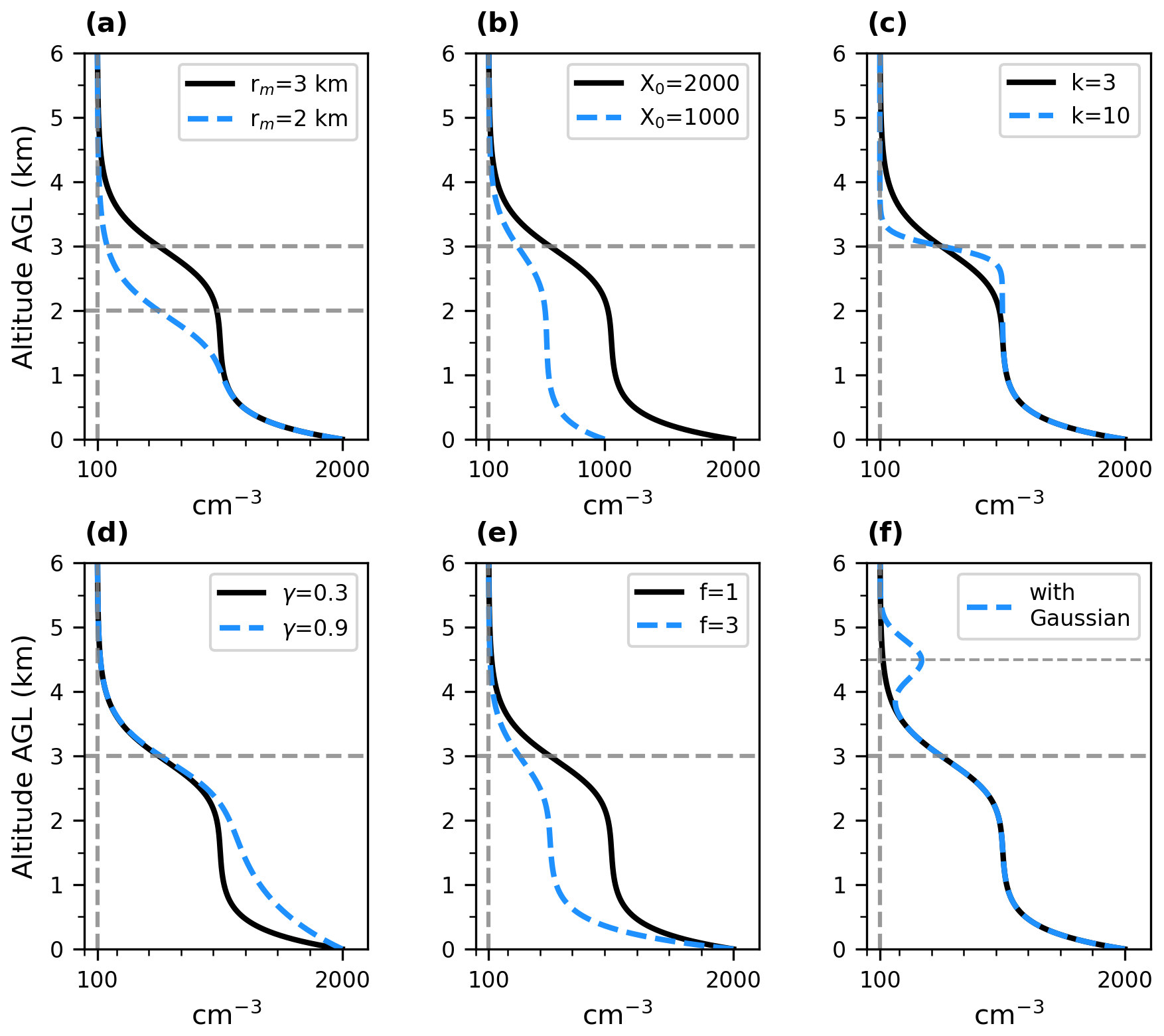
Figure 3 Effects of individual fitting function parameters on the aerosol vertical profile shape. Each panel varies one parameter while others are held constant. Solid black lines show the reference profile, and dashed blue lines show the parameter modified profiles. Horizontal gray dashed lines mark transition zone height r_m. Vertical gray dashed lines denote a constant concentration of 100 cm⁻³ (a) r_m shifts the height of the transition zone; (b) X₀ sets the surface concentration; (c) changing parameter k changes the sharpness of the transition; (d) changing parameter γ changes the shape of near surface decline in concentration; (e) changing parameter f influences the magnitude of the exponential decay; and (f) adds a Gaussian peak to represent an elevated aerosol layer.

Equation (1) provides a parameterization for aerosol concentration that decreases from the higher concentrations fixed near the surface to the cleaner air aloft through a single S-shaped transition. It allows for flexible control over the key observable features of the profile as shown in Fig. 3. To arrive at this equation, we define the transition zone as the altitude range over which aerosol concentration drops most rapidly from a well-mixed lower layer to the cleaner background aloft. The transition zone height, r_m, represents the midpoint of the transition zone and is obtained by fitting Eq. (1) to measured aerosol vertical distributions. Although r_m can coincide with the top of the planetary boundary layer, we use it here strictly as a metric of aerosol profile rather than as a direct boundary layer height estimate. In Eq. (1), X₀ controls the aerosol concentration at the surface, X_f represents the cleaner background concentration aloft, and k constrains how rapidly the aerosol concentration changes within the transition zone. The variables γ and f affect how aerosol concentration decreases with height below the transition zone. The parameters r_m and k are later compared with boundary layer height and potential temperature gradients to examine how boundary layer structure relates to aerosol vertical distribution.

In this study, γ is fixed at 0.3 to improve fit stability and reduce parameter trade-offs. Because γ and f both affect the profile curvature below the transition zone, allowing both parameters to vary can produce similar fits from different parameter combinations. Fixing γ reduces this trade-off, thereby providing more stable estimates of f and other parameters. To determine a fixed value to use for γ, Eq. (1) was first fitted with γ allowed to vary for all 313 aerosol profiles collected at AMF-1 during the six-month analysis period. The median fitted γ was 0.334, so we selected 0.3 as a representative fixed value near the center of the fitted distribution (Fig. S9a in the Supplement). Fitting Eq. (1) to the same profiles with γ fixed at 0.3 retained high goodness of fit, with a median R² of 0.980 (Fig. S9b in the Supplement).

While Eq. (1) models the monotonic, surface-anchored profiles typical of cases dominated by local emissions, it cannot represent distinct elevated aerosol layers that are separated from the boundary layer, such as those produced by long-range transport or secondary particle formation aloft. In this study, the parameters of Eq. (1) are constrained by near-surface aerosol measurements together with lidar-derived aerosol profiles. To represent elevated layers observed in the lidar profiles, one or more Gaussian peak terms can be added to Eq. (1). Each Gaussian is centered at the altitude of an observed elevated layer and providing a simple parametric description of that feature. To avoid overfitting, we use as few Gaussian terms as necessary. Elevated layers were identified by visual inspection of the lidar-derived aerosol concentration profiles and were counted only when a distinct local maximum above the surface-connected profile was separated from the lower aerosol layer by a relative local minimum. Specifically for this study, we allow at most two Gaussian terms when elevated layers are apparent. The fitting function with N elevated aerosol layers is given by:

$$\begin{array}{}\text{(2)}& \begin{array}{rl}{X}_{\text{aug}}\left(r\right)=& {\displaystyle \frac{X_{\mathrm{0}}-X_{\mathrm{f}}}{\mathrm{1}+f}}\cdot {\displaystyle \frac{\mathrm{1}+f{e}^{-\frac{r}{\mathit{\gamma }}}}{\mathrm{1}+{\left(\frac{r}{r_{\mathrm{m}}}\right)}^{r_{\mathrm{m}}k}}}\\ & +\sum _{j=\mathrm{1}}^N{A}_j\text{exp}\left(-{\displaystyle \frac{\mathrm{1}}{\mathrm{2}}}{\left({\displaystyle \frac{r-r_{\mathrm{c},j}}{{\mathit{\sigma }}_j}}\right)}^{\mathrm{2}}\right)+X_{\mathrm{f}}\end{array}\end{array}$$

Equation (2) adds N Gaussian terms to Eq. (1), each representing an elevated aerosol layer centered at altitude r_c,j with amplitude A_j and width σ_j. The value of N was selected as the minimum number of Gaussian terms needed to represent visually distinct elevated layers, with N=0, 1, or 2 corresponding to no elevated layer, one elevated layer, or two elevated layers, respectively. An example profile derived from Eq. (2) with a single Gaussian term is illustrated in Fig. 3f.

2.4 Boundary layer height determination

Boundary-layer height may contribute to aerosol profile shape and therefore may covary with the fitted parameters in Eq. (1). To compare the aerosol profiles with BLH, we use two BLH products from the Houston observational dataset from Lamer et al. (2024).

The first estimate, referred to as BLH-RiB, is derived from the bulk Richardson number (R_iB), which combines virtual potential-temperature stratification and horizontal wind to characterize their influences on turbulent mixing (Stull, 2012). BLH-RiB is assigned to the lowest altitude at which R_iB reaches 0.5 (Lamer et al., 2024).

The second estimate, referred to as BLH-LL, follows the potential-temperature approach adapted by Lamer et al. (2024) from Liu and Liang (2010). Each profile is first categorized as convective, stable, or neutral residual according to its near-surface potential-temperature structure. The boundary-layer top is then diagnosed using features appropriate to the identified regime. For convective and neutral-residual profiles, the method uses the increase in potential temperature from near the surface with its vertical gradient. For stable profiles, BLH-LL represents the top of the shallow stable layer, identified from the minimum potential-temperature gradient (Lamer et al., 2024; Liu and Liang, 2010).

3 Results

In the following sections, we present three case studies from the TRACER campaign to illustrate how boundary layer processes, driven by diverse meteorological conditions, affect aerosol vertical distributions, and explain the mechanisms behind their observed variability. The aerosol profiles and their variability are further quantified by fitting Eqs. (1) and (2) to the data.

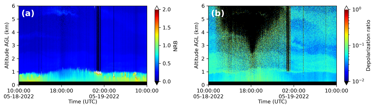
Figure 4 Micropulse lidar measurement from 10:00 UTC on 18 May to 10:00 UTC on 19 May 2022, at AMF-1 site (a) normalized relative backscatter time series and (b) linear depolarization ratio time series with signal to noise ratio > 3.

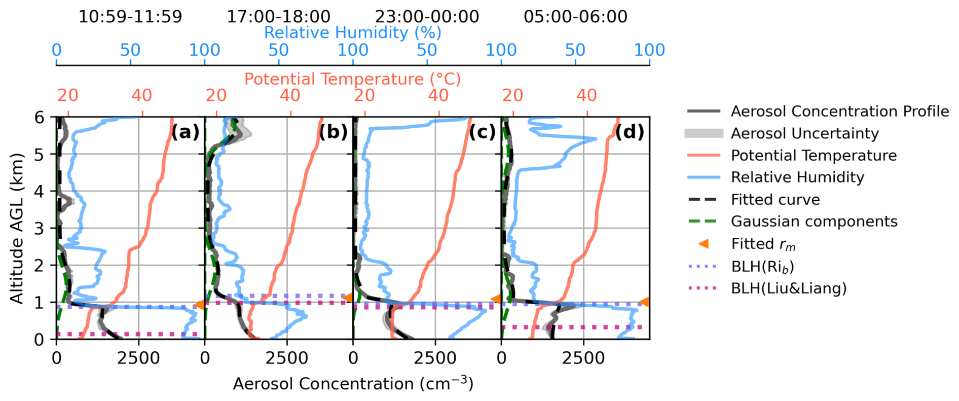
Figure 5 Retrieved vertical profiles of aerosol number concentration (gray solid lines), potential temperature profiles (solid red lines), relative humidity profile (solid blue lines), and curve fit aerosol vertical profile (dashed black lines) at the AMF-1 site on 18–19 May 2022. Green dashed lines indicate Gaussian components added to represent elevated aerosol layers. Orange triangles mark the fitted transition height r_m. BLHs determined by the bulk Richardson number and the Liu and Liang method are shown as purple and magenta dotted horizontal lines, respectively. The curve fit profile closely overlaps the measured number-concentration profiles, so the gray lines can be difficult to distinguish from the black dashed lines where agreement is good. Each panel corresponds to a one-hour averaging window in UTC time: (a) 10:59–11:59 on 18 May, panel (b) 17:00–18:00 on 18 May, (c) 23:00–00:00 across 18–19 May, and (d) 05:00–06:00 on 19 May.

3.1 Case study: Aerosol stratification below a strong capping inversion

The first case on 18–19 May 2022 showcases the evolution of the aerosol vertical profile within a well-mixed boundary layer capped by a strong temperature inversion. The largest normalized relative backscatter (NRB) is found close to the surface, forming a distinct boundary where it transitions to lower NRB around 1 km, above which elevated aerosol layers between 3 and 6 km are also visible (Fig. 4a). Figure 4b more clearly reveals elevated aerosol layers through the depolarization ratio. The aerosol layer below 1 km exhibits a smaller NRB and larger depolarization ratio during the daytime, which mirrors the evolution of surface relative humidity, as shown in Fig. S2 in the Supplement, where the relative humidity decreases from 100 % at nighttime to 50 % in the early afternoon. The larger relative backscatter and smaller depolarization ratios observed near the surface at night are due to greater humidity, causing aerosols to take up water and become larger and more spherical. In Fig. 4b, one elevated aerosol layer can be identified between 1 and 2.5 km, separated from the aerosol layer below 1 km. Relative humidity drops sharply around 1 km (Fig. 5), and aerosol aloft are therefore more likely dry and less spherical, which increases the depolarization ratio. HYSPLIT back trajectories (Fig. S5 in the Supplement) indicate that the low-level and 1–2.5 km layers were transported from over the Gulf of Mexico during the preceding 12–24 h. The pronounced relative humidity dependence of the depolarization ratio in these layers, together with the HYSPLIT results, is consistent with contributions from hygroscopic aerosol, such as sea salt aerosol or water soluble organic aerosol. Elevated aerosol layers between 3 and 6.6 km show large depolarization ratios, with the 5 km layer traced by 24 h HYSPLIT back trajectories to long range free tropospheric transport.

Aerosol, potential temperature, and RH profiles, as well as BLH estimates at different times of the day on 18–19 May 2022 are shown in Fig. 5. The four aerosol profiles throughout the day are similar. For all four profiles, aerosol concentrations are approximately 1500 to 2000 cm⁻³ near the surface and decrease sharply to less than 500 cm⁻³ above 1 km altitude. Equation (2) is used to fit to the aerosol vertical profiles (with fit parameters listed in Table S1 in the Supplement). All four potential temperature profiles in Fig. 5 show a strong inversion near 1 km, and BLH-RiB remains near this level throughout the day, closely matching the fitted transition zone height r_m. The alignment of the sharp decrease in aerosol concentration with the potential-temperature inversion is consistent with the stable layer limiting vertical mixing and maintaining the observed aerosol stratification. The RH profile also exhibits features that align with the aerosol distributions. Below 1 km, RH reaches around 90 % or higher except in the early afternoon (68.6 % at 17:00–18:00 UTC; Fig. 5b), and it drops sharply near 1 km at the primary aerosol-layer top. This pattern is consistent with boundary-layer turbulent transport shaping both moisture and aerosol distributions. Note that the influence of RH and hygroscopic growth on the aerosol lidar signal has already been accounted for in the retrieval of the aerosol vertical profile (Chen et al., 2025).

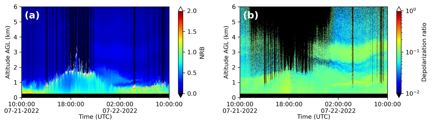
Figure 6 Micropulse lidar measurement from 10:00 UTC on 21 July to 10:00 UTC on 22 July 2022, at AMF-1 site (a) NRB time series (b) linear depolarization time series with signal to noise ratio > 3.

As described in Sect. 2.4, BLH-RiB and BLH-LL are based on different measurements and criteria. BLH-RiB is defined using a bulk Richardson-number threshold calculated from virtual potential-temperature and wind profiles, whereas BLH-LL is determined from regime-specific features of the potential-temperature profile alone. While BLH-RiB remains near the ∼ 1 km inversion described above, BLH-LL is much lower, 140 m in the early morning (10:59–11:59 UTC; Fig. 5a) and 320 m around midnight (05:00–06:00 UTC; Fig. 5d), consistent with a shallow nocturnal stable boundary layer near the surface. The two BLH estimates agree more closely in the early afternoon (17:00–18:00 UTC; Fig. 5b) and early evening (23:00–00:00 UTC; Fig. 5c). This separation between the shallow nocturnal BLH and the higher inversion is consistent with the formation of a residual layer. Aerosols that accumulate within the deeper daytime boundary layer often remain suspended above the much shallower nocturnal layer, forming a residual layer at night.

The aerosol vertical profile in this case study is strongly governed by boundary layer processes, with well-mixed near surface layers during the day and residual layering at night. The aerosol profile exhibits sharp stratification near inversion layers, and elevated aerosol layers persist aloft, decoupled from surface influences. The vertical distributions thus highlight the importance of diurnal boundary layer evolution in shaping aerosol structure.

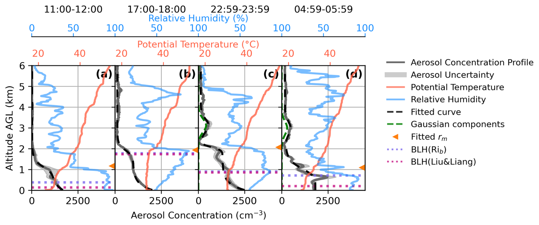
Figure 7 Measured vertical profiles of aerosol number concentration (gray solid lines), potential temperature profiles (solid red lines), relative humidity profile (solid blue lines), and curve fitted aerosol vertical profile (dashed black lines) at the AMF-1 site on 21–22 July 2022. Green dashed lines indicate Gaussian components added to represent elevated aerosol layers. Orange triangles mark the fitted transition height r_m. Boundary layer heights determined by the bulk Richardson number and the Liu and Liang method are shown as purple and magenta dotted horizontal lines, respectively. The curve fit profile closely overlaps the measured number-concentration profiles, so the gray lines can be difficult to distinguish from the black dashed lines where agreement is good. Each panel corresponds to a one-hour averaging window in UTC time: (a) 11:00–12:00 on 21 July, panel (b) 17:00–18:00 on 21 July, (c) 22:59–23:59 on 21 July, and (d) 4:59–05:59 on 22 July.

3.2 Case study: Aerosol profile under boundary layer development and collapse

The second case, recorded on 21–22 July 2022, demonstrates the evolution of the aerosol vertical structure during the development and collapse of the daytime boundary layer. Figure 6 shows the 24 h NRB and depolarization ratio measurements from the micropulse lidar, capturing the vertical structure of aerosols and clouds throughout the diurnal cycle. Figure S3 in the Supplement shows the corresponding surface meteorological measurements. As seen in Fig. 6a, shallow cumulus clouds developed during the local morning and extended to just below 2 km by early afternoon (18:00 UTC), marking the growth of the daytime boundary layer, whose top is often associated with boundary layer cumulus cloud top (Stull, 2012). Around 18:00 UTC, surface winds shifted from southwesterly to easterly, accompanied by a sudden increase in RH (Fig. S3), marking a change in near-surface air-mass influence. By late afternoon, around 22:00 UTC, banded and optically thick cirrus moved over the site (shown in Fig. S6 in the Supplement). This coincided with reduced vertical mixing and an early collapse of the mixed layer, as indicated by a decrease in BLH from Fig. 7b to c. An elevated aerosol layer between approximately 2.5 and 4 km is visible in Fig. 6b, which shows larger depolarization ratios in the 0–2 and 2.5–4 km ranges, separated by a layer of smaller depolarization ratio in between. The elevated aerosol layer becomes more distinct in the evening hours and persists into the night. A similar elevated layer between around 2.5 and 4 km is also faintly visible in the backscatter signal of Fig. 6a. The separation between the low-level aerosol layer and the elevated layer indicate possible stratification and limited vertical mixing between these layers during the observation period. HYSPLIT back trajectories (Fig. S7 in the Supplement) show the ∼ 3 km layer arrived from the east along the Gulf Coast, unlike the low-level air mass, indicating the elevated layer is decoupled from the boundary layer and likely has a distinct source, potentially from long-range transport.

Figure 7 presents aerosol vertical profiles, potential temperature, relative humidity, and BLHs at four different times. Surface aerosol concentrations remain consistently large throughout the 24 h period, ranging approximately from 1700 to 2500 cm⁻³. Equations (1) and (2) are used to curve fit the aerosol vertical profiles, as illustrated in dashed black lines in Fig. 7. The profiles follow an S-shaped decrease in concentration, with the transition zone height r_m diagnosed from the fitted curve. One dominant aerosol layer is observed in early morning (11:00–12:00 UTC; Fig. 7a) and early afternoon (17:00–18:00 UTC; Fig. 7b) shown in Fig. 7a and b. In the early morning (11:00–12:00 UTC; Fig. 7a), r_m is near 1 km, indicating the nighttime residual aerosol layer. By early afternoon (17:00–18:00 UTC; Fig. 7b), r_m rises to just below 2 km as the mixed layer deepens, as indicated by BLH-RiB and BLH-LL, which closely agree and coincide with r_m. The potential temperature structure is consistent with this evolution. In Fig. 7a, a modest temperature inversion near 1 km aligns with the sharp drop in aerosol concentration, suggesting limited vertical mixing. In Fig. 7b, the height of the inversion increases, with the inversion occurring just below 2 km, consistent with the deeper mixed layer. Above these heights, aerosol concentrations remain small, with minor aerosol features aloft. As seen in Fig. 7c, in the early evening (22:59–23:59 UTC), both BLH-RiB and BLH-LL dropped to around 0.9 km and coincide with a temperature inversion, consistent with early boundary-layer collapse. However, r_m remained elevated at around 2 km, suggesting a decoupling between the BLH and r_m as the boundary layer collapsed. At midnight (04:59–05:59 UTC; Fig. 7d), the r_m remained around 1 km, while BLH-RiB (0.7 km) and BLH-LL (0.2 km) both fell below r_m. The sharpness of the transition zone is also weaker at midnight (04:59–05:59 UTC; Fig. 7d), with the lowest curve fitted k on this day (Table S2 in the Supplement). The diurnal aerosol vertical profile evolution shows that aerosol vertical structure is coupled to the boundary layer during its growth but not its collapse. This phenomenon is typical for the nighttime boundary layer, when the residual layer remains aloft as a new nocturnal boundary layer forms (Bourgeois et al., 2018). Together, the elevated r_m after BLH collapse and the weaker nighttime transition indicate that abrupt boundary layer collapse before sunset can decouple the aerosol layer from the surface before the nocturnal boundary layer is fully established. In addition, the disagreement between BLH-RiB and BLH-LL in Fig. 7a and d reflects the different sensitivities of the two BLH diagnostics under stable nighttime conditions.

In addition to the low-level aerosol structure discussed above, elevated aerosol layers between 2.5 and 4 km can be seen in early evening (22:59–23:59 UTC; Fig. 7c) and at midnight (04:59–05:59 UTC; Fig. 7d). These layers remain separated from the lower aerosol layer by a region of lower aerosol concentration, indicating limited merging between the elevated and lower layers during this period. These layers also coincide with a high-RH layer aloft and are bounded by upper-level inversions, consistent with stratification helping maintain vertical separation. While these profiles suggest distinct layers, they cannot entirely rule out some degree of downward mixing; furthermore, the co-location with RH and inversions does not establish causality or rule out a shared driver.

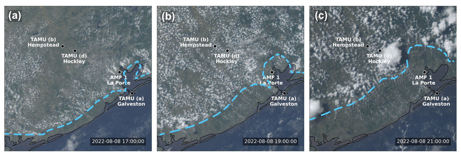
Figure 8 GOES16 Geocolor imagery on 8 August 2022, at 17:00 (a), 19:00 (b), and 21:00 UTC (c). The sea breeze front is marked in blue dashed lines. The campaign sites are labeled in white text.

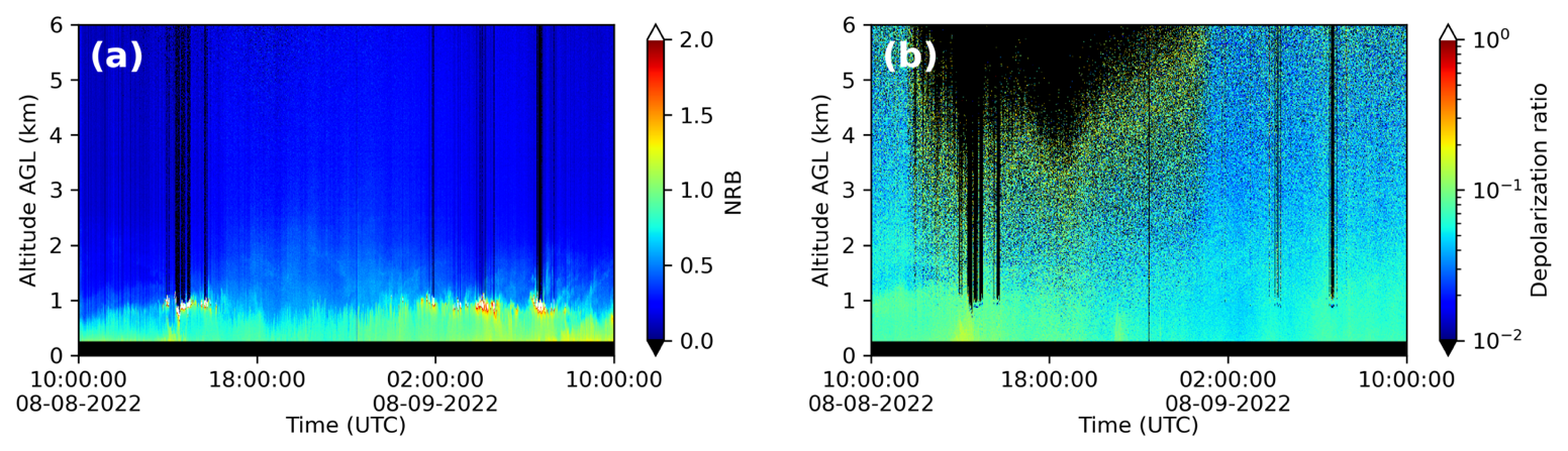
Figure 9 Micropulse lidar measurement from 10:00 UTC on 8 August to 10:00 UTC on 9 August 2022, at AMF-1 site (a) NRB time series (b) linear depolarization time series with signal to noise ratio > 3.

3.3 Case study: Sea breeze circulation and airmass impact on aerosol vertical distributions

The third case, on 8–9 August 2022, showcases the evolution of the aerosol vertical profile under the influence of a sea breeze circulation. On this day, the ROAM-V sampled at multiple TAMU sites: it began measurements in Galveston in the morning and later relocated inland to Hempstead, while AMF-1 operated continuously at La Porte. To visualize the progression of the sea-breeze front relative to the active ROAM-V location and AMF-1, Fig. 8 presents GOES-16 Geocolor imagery (Miller et al., 2020). The sea breeze front was identified based on the characteristic inland advancing cumulus cloud bands visible in the satellite imagery (Planchon et al., 2006; Sharma et al., 2024). The sea breeze front marks a sharp boundary that separates cooler, moister maritime air along the coast from the continental air farther inland. According to Fig. 8, by about 17:00 UTC, the sea breeze front had already passed the TAMU Galveston site but was only just beginning to move across the AMF-1 site at La Porte. By 21:00 UTC, the sea breeze front had moved past the coastal sites at Galveston and La Porte but had not yet reached the inland TAMU Hempstead site.

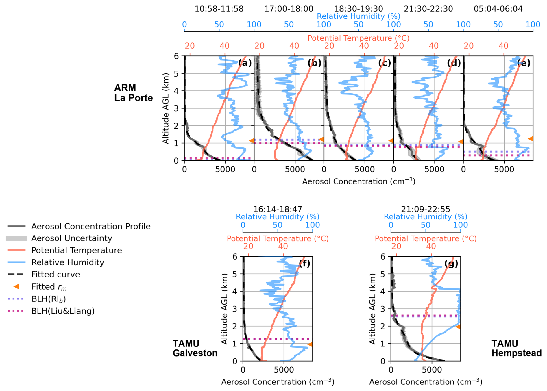
Figure 10 Measured vertical profiles of aerosol number concentration (gray solid lines), potential temperature profiles (solid red lines), relative humidity profile (solid blue lines), and curve fitted aerosol vertical profile (dashed black lines) at the AMF-1 site and two TAMU sites on 8–9 August 2022. Orange triangles mark the fitted transition height r_m. Boundary layer heights determined by the bulk Richardson number and the Liu and Liang method are shown as purple and magenta dotted horizontal lines, respectively. The curve fit profile closely overlaps the measured number-concentration profiles, so the gray lines can be difficult to distinguish from the black dashed lines where agreement is good. The averaging windows are given below in UTC. AMF-1 site: (a) 10:58–11:58 on 8 August, (b) 17:00–18:00 on 8 August, (c) 18:30–19:30 on 8 August, (d) 21:30–22:30 on 8 August, and (e) 05:04–06:04 on 9 August. TAMU Galveston site (f) 16:14–18:47 on 8 August. TAMU Hempstead site (g) 21:09–22:55 on 8 August.

As seen in Fig. 9, no notable elevated aerosol layers are observed on this day. The NRB field shows some variability near 1 km throughout the day, but the depolarization ratio does not show a distinct separation at this altitude. This suggests that the aerosol structure is more continuous than in the previous cases. Together with the weaker inversion shown in Fig. 10, this pattern is consistent with weaker stratification and more effective vertical mixing within the lower atmosphere.

Aerosol concentration, potential temperature, and RH profiles, as well as BLHs at selected times at the AMF-1 site are shown in Fig. 10. Corresponding profiles measured at the TAMU Galveston and Hempstead sites are also included (marked in Fig. 10). The TAMU profiles use longer averaging windows because the lidar measurements required longer temporal averaging to obtain enough cloud-free profiles for the retrieval. For both ARM and TAMU Galveston sites, the potential temperature profiles have a distinctly different vertical structure compared to the previous two cases, featuring a much weaker inversion at around 0.8 km and less inhibition to vertical mixing. The aerosol profiles also appear less structured, with a smoother vertical gradient and no clear separation between layers as seen in the previous two cases. Since measurements from multiple sites are available on this day, we can investigate how the sea breeze circulation shapes aerosol vertical distributions across the urban coastal area. This analysis compares the observed aerosol vertical profiles, the transition zone height r_m derived from Eq. (1) curve fit, and the BLHs obtained from radiosonde measurements across the maritime and continental side of the sea breeze front.

At the AMF-1 site, the near-surface aerosol concentration increases from approximately 4400 cm⁻³ in the early morning (10:58–11:58 UTC; Fig. 10a), to 7200 cm⁻³ around noon (17:00–18:00 UTC; Fig. 10b), accompanied by higher concentration aloft. During this period, the BLH increased from below 0.2 km to approximately 1 km. Although boundary layer development may enhance mixing and dilution, local emissions or transport of aerosol rich air may have contributed to the observed increase. Shortly after, concentrations begin to decrease throughout the late afternoon and evening, reaching a minimum of around 2900 cm⁻³ in the late afternoon (21:30–22:30 UTC, Fig. 10d). The decline in concentration coincides with the arrival of maritime air south of the sea breeze front, replacing the earlier continental air mass. Easterly to southeasterly surface winds at AMF-1 (Fig. S4a in the Supplement) during this period are consistent with the increasing maritime influence. Aerosol concentrations aloft follow a similar trend, with larger concentrations around noon (17:00–18:00 UTC; Fig. 10b) that gradually decline into the evening. The fitted transition zone height r_m at the AMF-1 site is around 1.2 km throughout the day. Both BLH-RiB and BLH-LL agreed well, increasing from < 0.2 km in early morning (10:58–11:58 UTC; Fig. 10a) to about 1 km in early afternoon before gradually decreasing toward midnight (05:04–06:04 UTC on 9 August; Fig. 10e) . The BLH remained shallow, peaking near 1 km after the sea breeze passage. The weak mixed-layer growth may explain the limited change in r_m. The sea breeze and the HYSPLIT back trajectories (Fig. S8 in the Supplement) indicate that the aerosol sampled at AMF1 were primarily of maritime origin.

At the TAMU Galveston site, from late morning to early afternoon (16:14–18:47 UTC; Fig. 10f), the aerosol vertical distributions resemble that observed at the AMF1 site in the afternoon (18:30–19:30 UTC; Fig. 10c), and the fitted transition zone height r_m at Galveston closely matches the r_m at the AMF1 site around noon (17:00–18:00 UTC; Fig. 10b) at around 1 km (see Tables S3 and S4 in the Supplement). This similarity reflects the influx of maritime air behind the sea breeze front, which carries relatively cleaner marine air and establishes a boundary layer structure comparable at both locations once the sea breeze front has passed. HYSPLIT trajectories indicate Galveston air also arriving from the southeast over the Gulf, explaining its close resemblance to AMF-1 once the sea breeze has passed (Fig. S8 in the Supplement). At the TAMU Hempstead site in the late afternoon (21:09–22:55 UTC; Fig. 10g), aerosol concentrations throughout the profile were greater than at the coastal sites, and the fitted transition height r_m was about 1.94 km. The fitted r_m at the Hempstead site is also closer to the BLH, which is at around 2.5 km. The greater aerosol concentration and deeper transition region height are characteristic of the continental air mass that persists inland, rich in urban and biogenic emissions and less influenced by marine dilution. In addition, HYSPLIT trajectories for Hempstead remain near the surface until close to arrival of the sea breeze front (Fig. S8 in the Supplement), supporting the interpretation that the site was influenced by a local or continental air mass, which helps explain the larger aerosol concentration and higher r_m observed there.

The comparison between the aerosol vertical distributions at different sites and times of the day reveals that the aerosol vertical distributions can have strong spatial heterogeneity, especially when there is a sea breeze circulation. During TRACER, near-surface aerosol properties differed systematically between polluted-marine and continental airmasses (Thompson et al., 2025a). This case study shows that, in a coastal urban environment like the Greater Houston area, the aerosol vertical distributions can be affected by sea breeze circulation and air mass transitions.

3.4 Relationship between Boundary Layer Height and Aerosol Vertical Profile

The AMF-1 deployment in the Greater Houston area offers a large dataset to study which environmental predictors are associated with and can potentially be used to predict the shape of aerosol vertical profiles. Six months of data from March 2022 to September 2022 were curve fitted using Eqs. (1) or (2). Profiles that were first fitted with Eq. (1) with R² < 0.98 and were visually classified as containing an elevated aerosol layer were then refit using Eq. (2) with one or two Gaussian terms. A profile was visually classified as having an elevated layer when it showed a distinct local maximum in aerosol concentration above the low-level aerosol layer and was separated from it by a relative local minimum. After model selection, only profiles with final fit quality R² > 0.98 were retained for the statistical analysis to ensure that the fitted parameters represented well-resolved profile structure. Overall, 157 of 313 profiles met this strict quality criterion. 34 out of 157 selected profiles are classified as containing elevated aerosol layers and are fitted with Eq. (2). The frequency distributions of fitted parameters are presented in the supporting information in Fig. S10 in the Supplement. As shown qualitatively in the case studies, we observe that BLH and r_m may have a positive correlation during the daytime. Comparing the case studies, a more abrupt transition from the low-level aerosol-rich layer to the air aloft, quantified by a larger k, is associated with stronger potential-temperature inversions. As we observed, the aerosol profiles on 18–19 May 2022 exhibit both a tighter transition zone and a steeper transition (larger k) than the profiles on 8–9 August 2022. Motivated by these patterns, we compare BLH and stability with the curve-fitted transition height r_m and the shape parameter k. For reference, we also provide the corresponding BLH–r_m and stability–k scatter plots obtained when Eq. (1) is applied to all profiles (i.e., without elevated-layer refitting) in the Supplement (Figs. S11 and S12).

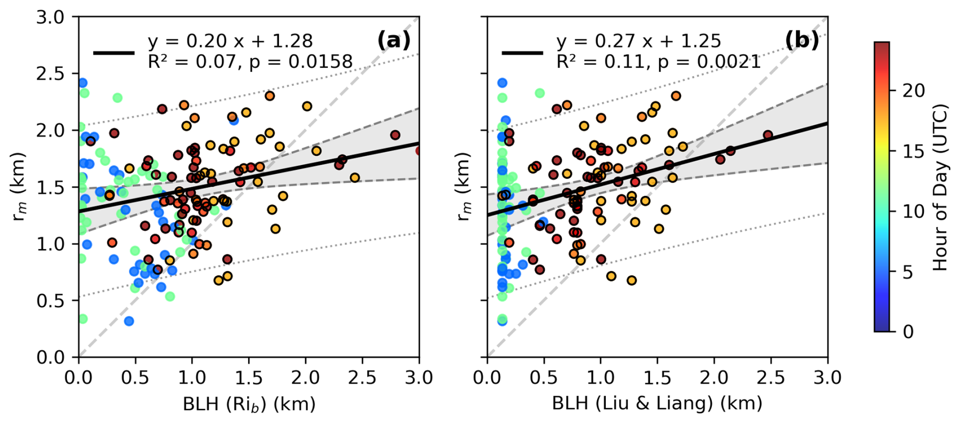
Figure 11 (a) Comparison between boundary layer heights derived from the bulk Richardson number method and the curve fitted r_m (b) Comparison between BLHs obtained with the Liu and Liang (2010) thermodynamic method and the r_m. The scattered points are color coded by the hour of day (UTC), with warmer colors corresponding to daytime hours. Points corresponding to daytime hours (12:00–23:00 UTC) are additionally highlighted with black outlines. The linear regression line is shown in a solid black line and is only performed on daytime datapoints. The gray band bounded by dashed lines shows the 95 % confidence interval for the fitted mean regression line, while the dotted gray lines bound the 95 % prediction interval for individual observations.

In Fig. 11, we compare the thermodynamically determined BLH from radiosonde data with the curve fitted transition zone height r_m to examine how the BLH covaries with structure of the aerosol vertical profiles using available data from March to September 2022 measured at the AMF-1 site. Comparison between the curve fitted transition height r_m and BLH shows that r_m tends to be systematically higher, as most data points lie above the 1:1 reference line. This overestimation may reflect the fact that aerosol layers often extend above the diagnosed boundary layer, particularly when the boundary layer is not well mixed. As shown in Fig. 11, BLH values are greater during the daytime and can reduce the discrepancy between r_m and BLH. In contrast, during nighttime or under stable stratification conditions, the diagnosed BLH becomes much shallower, while elevated aerosol layers may persist. In these cases, the Liu and Liang (2010) method appears more effective at capturing shallow stable boundary layers than the Richardson number method, potentially providing a closer match to the aerosol-defined transition height during daytime.

We performed linear regression analysis using daytime data only, comparing the fitted aerosol transition height r_m with BLH derived from both the Richardson number and Liu and Liang methods. We find a weak but statistically significant positive correlation between the curve fitted transition height r_m and the BLH. The relationship is stronger when using the BLH-LL (R² = 0.11, p = 0.0021) than when using the BLH-RiB (R² = 0.07, p = 0.0158). The positive correlation indicates that higher BLHs are generally associated with deeper aerosol transition heights, suggesting that BLH plays a contributing role in shaping the aerosol vertical structure. However, the relatively low R² shows that the BLH only explains a small fraction of the variability in r_m. Therefore, the regression is used here to summarize the observed correlation between BLH and r_m and to assess the explanatory power of BLH. Based on the results, the regression should not be used as a standalone predictor of aerosol transition height.

The limited explanatory power of BLH likely reflects several contributing factors. First, the aerosol vertical profile is shaped not only by the instantaneous thermodynamic structure, but also by the boundary layer's recent evolution. As seen in the case study of 21 July 2022, during boundary layer growth, surface emitted aerosols become mixed throughout a deepening layer. As BLH decays, previously mixed aerosols can remain aloft even as the boundary layer becomes shallow, causing a mismatch between BLH and r_m. Second, aerosol layers from long range transport can reside over the local boundary layer and later subside and merge with near surface aerosol layer. Even with additional Gaussian peaks, the fitting routine may not always cleanly separate the transported signal from locally emitted aerosols. And finally, uncertainties in both BLH diagnostics and the aerosol curve fitting, particularly under weak stratification or merged layers, can mask the link between BLH and r_m.

In conclusion, although BLH exhibits a weak but statistically significant positive correlation with the fitted transition height r_m, BLH explains only a small fraction of the variability in r_m. This result indicates that BLH alone cannot reliably determine the depth of the near-surface aerosol layer or the overall structure of the aerosol vertical profile.

3.5 Relationship between Thermodynamic Stability and Aerosol Vertical Profile

We then examine whether the local vertical gradient in potential temperature (i.e., the static stability) can help explain variations in k. Since atmospheric stability influences vertical mixing and stratification, a stronger gradient in potential temperature is expected to be associated with a steeper vertical aerosol gradient, k, at the transition zone, r_m. The local maximum vertical gradient of potential temperature ($\mathrm{d}\mathit{\theta }/\mathrm{d}z$) was calculated within ± 100 m of the fitted transition height r_m, using smoothed radiosonde profiles to reduce high frequency noise. The smoothing was performed with a Gaussian kernel with a full width at half maximum of 100 m, consistent with common boundary layer profiling practice of applying vertical averaging at a scale of tens of meters (Bhimireddy and Kristovich, 2024). The comparison between static stability and k is shown as a scatterplot in Fig. 12.

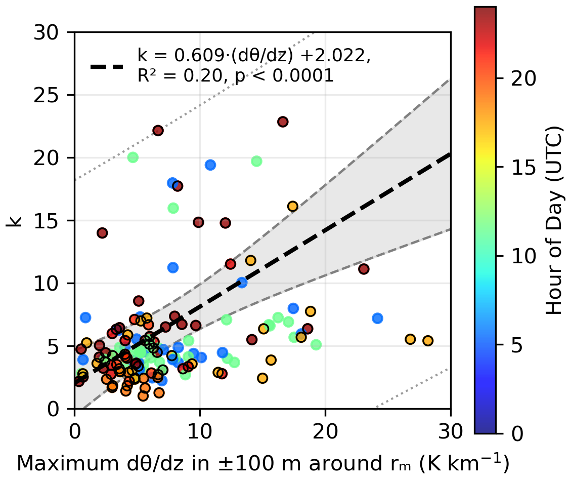
Figure 12 Comparison between local maximum potential temperature gradient ($\mathrm{d}\mathit{\theta }/\mathrm{d}z$, evaluated within ± 100 m around curve fitted r_m) and curve fitted k results based on AMF-1 data. Points corresponding to daytime hours (12:00–23:00 UTC) are additionally highlighted with black outlines. The linear regression line is shown in a dashed black line. The gray band bounded by dashed lines shows the 95 % confidence interval for the fitted mean regression line, while the dotted gray lines bound the 95 % prediction interval for individual observations.

A statistically significant (p ≪ 0.01) and limited positive correlation (R² = 0.20) is found between the potential temperature gradient at r_m and the curve-fitted transition sharpness parameter k. Sensitivity tests using different Gaussian smoothing scales and search-window widths show that the positive relationship remains, although the slope and R² vary with the operational definition of the local stability metric (Fig. S13 in the Supplement). This result shows that the local atmospheric stability near r_m appears to contribute to the shape of the aerosol profile but does not fully define it. A possible physical explanation is that stronger stability can suppress vertical exchange across the aerosol transition zone, allowing a sharper aerosol concentration gradient to persist. In contrast, weaker stability may permit more gradual mixing between the lower aerosol rich layer and cleaner air aloft, resulting in a more gradual transition zone and smaller k values. Because the correlation is limited, we interpret $\mathrm{d}\mathit{\theta }/\mathrm{d}z$ near r_m as a partial constraint on aerosol stratification rather than as the only control on k. Additional variability may arise from transported aerosol mixing with the lower layer, residual uncertainty in the hygroscopic-growth correction, and the history of boundary-layer growth, collapse, and residual-layer formation.

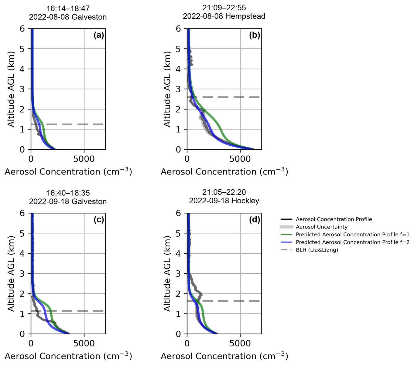
Figure 13 Demonstration of aerosol vertical profile prediction with TAMU data using the curve fitting equation and parameterization derived from AMF-1 site observations. (a) 16:14–18:47 UTC on 8 August 2022 at Galveston site, (b) 21:09–22:55 UTC on 8 August 2022 at Hempstead site (c) 16:40–18:35 UTC on 18 September 2022 at Galveston site (d) 21:05–22:20 UTC on 18 September 2022 at Hockley site. The aerosol profile is shown in black. The predicted profiles using f=1 are shown as the green line, and the predicted profiles using f=2 are shown as the blue line. The BLH-LL is marked with a horizontal gray dashed line.

3.6 Demonstration of Aerosol Vertical Profile Prediction

Using the significant but weak empirical relationships established above, we next demonstrate aerosol vertical-profile prediction using these variables in place of vertical lidar measurements, as shown in Fig. 13. Because BLH-LL showed a slightly stronger empirical relationship with r_m than BLH-RiB in the daytime AMF-1 analysis (Fig. 11), the BLH-LL is used in the following analysis. The transition height r_m is estimated using the linear regression relationship with the Liu and Liang (2010) based BLH, expressed as r_m = 0.27 × BLH + 1.25 km. The sharpness of the transition zone k is then estimated as k = 0.609 × $(\frac{\mathrm{d}\mathit{\theta }}{\mathrm{d}z}{)}_{max,r_{\mathrm{m}}\pm \mathrm{100}\mathrm{m}}$ + 2.022. γ is set as 0.3, consistent with the previous curve fitting. Since a predictive relationship was not found for f, fixed values of f=1 and f=2 are selected for testing, guided by the distribution shown in Fig. S10, where the mode of f is centered around 1.1. The aerosol concentration measured on the surface is used for X₀. X_f is set to 150 cm⁻³, as a representative background value close to the overall median obtained from the quality-controlled AMF-1 profile fits. The prediction equation then becomes:

$$\begin{array}{}\text{(3)}& \begin{array}{rl}& X\left(r\right)={\displaystyle \frac{X_{\mathrm{0}}-\mathrm{150}}{\mathrm{1}+f}}\\ & \times {\displaystyle \frac{\mathrm{1}+f{e}^{-\frac{r}{\mathrm{0.3}}}}{\mathrm{1}+{\left(\frac{r}{\mathrm{0.27}\times \text{BLH}+\mathrm{1.25}}\right)}^{\left(\mathrm{0.27}\times \text{BLH}+\mathrm{1.25}\right)\left(\mathrm{0.609}\times {\left(\frac{\mathrm{d}\mathit{\theta }}{\mathrm{d}z}\right)}_{max,r_{\mathrm{m}}\pm \mathrm{100}\mathrm{m}}+\mathrm{2.022}\right)}}}\\ & +\mathrm{150}\end{array}\end{array}$$

The TAMU coastal and inland site's aerosol vertical profiles for 8 August and 18 September were chosen for the demonstration. The TAMU site was not included in the derivation of the empirical relationships from the AMF-1 dataset, allowing the demonstration to test how the AMF-1-derived relationships perform when applied to profiles from other sites. Although the predictive relationships for r_m and k are only weak to moderate, the demonstration is useful for showing both what profile features can be approximated from these variables and where the approach breaks down, particularly in situations where direct vertical measurements are unavailable.

To quantify the profile-level uncertainty in this demonstration, we calculated the normalized RMSE between the predicted and lidar-retrieved aerosol concentration profiles for each case (Table S5 in the Supplement). The 8 August cases show lower errors when f=2 is used, with normalized RMSE values of 41.7 % at Galveston and 19.5 % at Hempstead, compared with 72.3 % and 56.7 % when f=1 is used. In contrast, the 18 September cases retain larger errors even when f=2 is used, with normalized RMSE values of 59.5 % at Galveston and 48.0 % at Hockley. This result indicates that the accuracy of the predicted profile depends strongly on reliable estimation of r_m, consistent with the weak BLH–r_m relationship shown in Fig. 11. This indicates that BLH alone is not a strong predictor of r_m. Uncertainty in the estimated r_m also affects the altitude range used to determine the temperature gradient and therefore the estimated k. These linked uncertainties may affect both the location and sharpness of the transition in the predicted aerosol profile. Thus, an accurate r_m is crucial for an accurate estimate of k. Additionally, the factor f has a strong influence on the shape of the aerosol profile and thus requires further investigation.

Our analysis uses a single retrieved aerosol number concentration profile based on the assumption that the surface aerosol is representative aloft, although particles of different sizes and composition may have different vertical distributions. Tethered balloon measurements during TRACER showed variability in aerosol sizes and composition with height, although they were not co-located with our lidar observations (Mei et al., 2026). Differences in physicochemical properties do affect the conversion from lidar backscatter to number concentration and, consequently, affect the fitted profile shape and its relationship with BLH and atmospheric stability. However, the available measurements for this study do not allow us to determine how accounting for these vertical variations would change our result.

4 Conclusion

In this work, we investigated how the vertical distributions of aerosols are related to boundary layer characteristics in a coastal urban environment, using data collected during the 2022 TRACER campaign in Greater Houston, Texas. We first developed an empirical model to describe aerosol vertical profiles from lidar observations, then compared the fitted profiles with thermodynamic profiles to assess how boundary layer processes affect aerosol vertical profiles. We examined case studies to illustrate how processes such as convective growth, the nocturnal stable boundary layer, and sea breeze circulation influence aerosol vertical structure. We also analyzed six months of data to evaluate the statistical relationships of aerosol profile features with BLH and static stability and demonstrated a preliminary framework for predicting aerosol profiles based on these variables.

In addressing our research goals, we find that the typical aerosol vertical profile in the Greater Houston coastal urban environment is S-shaped, with largest concentrations near the surface, relatively constant concentrations in the lowest 1–2 km above the surface layer associated with vertical mixing in the boundary layer, and a sharp decrease in a “transition zone”, which is often (but not always) at or above the boundary layer capping inversion; at nighttime, a residual layer of aerosol remains aloft, above the stable nocturnal boundary layer. This S-shape becomes more pronounced under stronger inversions or more stable boundary layer conditions, which suppress vertical mixing and sharpen the aerosol transition zone. Boundary layer processes, including convective atmospheric boundary-layer development, collapse, and sea breeze-driven circulation influence the shape of the aerosol profile, as demonstrated in our case studies and six-month analysis. We demonstrate that aerosol vertical profiles are only weakly related to BLH and thermodynamic stability. Though much of the variance is unexplained by these variables, they may still offer a practical framework for predicting aerosol vertical profile when airborne or lidar measurements are not available. These findings highlight the relationship between boundary layer properties and aerosol vertical distributions and establish a physically grounded basis for future profile prediction. The aerosol vertical profile fitting function developed in this study can also be applied to parameterize aerosol vertical profiles in numerical weather or climate models or provide constraints for remote sensing retrieval algorithms.

Our findings corroborate previous observations linking the aerosol vertical profile to boundary-layer structure (Sun et al., 2024; Li et al., 2022; Ware et al., 2016; Thomas et al., 2019; Prasad et al., 2022). However, most lidar studies have used optical profiles like the extinction coefficient profile, which are strongly influenced by hygroscopic growth in humid air. Because moisture is also controlled by boundary-layer processes, extinction-based metrics can overestimate the link to those processes by reflecting particle growth rather than actual concentration changes. We instead apply a correction for hygroscopic growth to backscatter profiles, reducing humidity-related biases and providing a clearer view of how the boundary layer processes shape aerosol vertical distributions.

One caveat is that these fitted relationships and parameter values are derived from a limited set of cases in the Houston coastal–inland regime during TRACER, and their applicability to other seasons, locations, and boundary-layer regimes remains uncertain. A logical next step is to apply the same curve-fitting framework at other ARM sites and evaluate how the fitted parameters relate to meteorological conditions across a broader range of regimes. Also, incorporating the evolution of the boundary layer over the preceding several hours into aerosol vertical-profile predictions, rather than relying solely on conditions at the time of measurement, may improve predictive skill. This is motivated by our finding that the BLH at the time of measurement is a weak predictor of aerosol vertical structure. Another improvement would be to incorporate long-term in situ sampling, for example, using tethered balloons or small drones to capture the behavior of ultrafine aerosols which are not detectable by an elastic lidar. In addition, the decay parameters γ and f, which control how sharply concentration decreases with height below r_m, remain loosely constrained and likely reflect the combined effects of turbulent mixing, entrainment at the boundary-layer top, surface emissions, gravitational settling, and boundary layer stability.