Assessment of methane emissions from European countries using satellite and surface observations

Europe is a global leader in mitigating methane emissions through comprehensive policies, including the EU Methane Strategy and commitments under the Global Methane Pledge. National bottom-up inventories are widely regarded as high quality; however, atmospheric observations remain essential for independent verification and tracking emission reductions. Here, we present a multi-year (2019–2023) top-down assessment of European methane emissions using a Bayesian inversion of satellite observations from TROPOMI and surface measurements from ICOS. Analysis of observational constraints shows that surface measurements provide the dominant information, while satellite observations offer complementary coverage in regions not covered by the surface network. The inversion estimates total European methane emissions at 25.7 Tg yr⁻¹, including 22.5 Tg yr⁻¹ from anthropogenic sources, which is 1.0 Tg yr⁻¹ higher than the prior inventory. The upward adjustments are likely associated with livestock and waste emissions in central and western Europe, partly offset by lower fossil fuel emissions in the North Sea. National emissions for the Netherlands, Germany, and Italy are 18 %–80 % higher than the values reported to the UNFCCC. The inversion also reveals an overall decline in anthropogenic emissions, with a linear trend of −0.25 Tg yr⁻². While consistent in magnitude with the prior estimate, the inversion shows a distinct spatial pattern: increases in livestock and waste emissions in western Europe contrast with decreases in fossil fuel production regions such as the North Sea and Poland. These findings highlight the value of atmospheric observations for evaluating methane inventories and informing climate policy.

1 Introduction

Methane (CH₄) is a strong greenhouse gas with a global warming potential ∼ 30 times that of CO₂ over 100 years. Increases in atmospheric methane concentrations since industrialization result in 0.54 W m⁻² effective radiative forcing, making it the second most important anthropogenic greenhouse gas after carbon dioxide (CO₂) (IPCC, 2021). Methane is emitted from various anthropogenic sources including fossil fuel production and use (oil, gas, and coal), agriculture (livestock and rice cultivation), and waste management (landfills and wastewater) (Fu et al., 2024; Saunois et al., 2020). Natural sources, dominated by wetlands, are also main contributors to the global methane budget (Kirschke et al., 2013; Zhang et al., 2023). Rapid reduction of methane emissions is a critical strategy for mitigating near-term warming, creating a crucial window for implementing long-term deep decarbonization (Nisbet et al., 2020; Szopa et al., 2021).

Europe has positioned itself as a global leader in methane mitigation. The methane mitigation policy of the European Union (EU) is anchored in the EU Methane Strategy (2020) and its commitment to the Global Methane Pledge, which aims for a 30 % reduction in global methane emissions by 2030 relative to 2020 levels. The EU adopted the landmark Methane Regulation (EU) 2024/1787 in May 2024, which mandates source-level measurement, reporting, and verification (MRV), requires frequent leak detection and repair (LDAR), prohibits routine venting and flaring, and introduces a framework for methane intensity requirements for domestic operations and energy imports into the EU (European Union, 2024). To address the agriculture and waste sectors, the revised Industrial and Livestock Rearing Emissions Directive (IED 2.0) imposes binding emission controls on the largest livestock farms, while the Landfill Directive mandates a reduction of municipal waste in landfills to 10 % by 2035.

Accurate quantification of methane emissions is critical for implementing policies and verifying progress. Under the Paris Agreement's enhanced transparency framework, European countries submit national greenhouse gas inventories to the UNFCCC on a regular basis. Many countries employ high-tier, methodologically advanced accounting practices in compiling these inventories, reflecting Europe's leading role in the development of reporting systems (EEA, 2024). However, persistent uncertainties from unaccounted emission sources or methodological biases necessitate independent verification. Top-down approaches, which infer emissions from atmospheric observations using inverse modeling, offer a powerful, objective complement to traditional bottom-up inventories (Houweling et al., 2017; Jacob et al., 2022; Wang et al., 2025; Worden et al., 2022; Zhang et al., 2021). Pioneering efforts, such as those by the United Kingdom, have been made to incorporate atmospheric verification into official national greenhouse gas inventory reporting (Manning et al., 2011).

The top-down approach relies on atmospheric observations. Satellite observations from GOSAT and TROPOMI have been widely used to estimate emissions at regional and national scales across diverse geographies (e.g., Shen et al., 2022; Zhang et al., 2020; Hancock et al., 2025; Chen et al., 2022, 2023; Liang et al., 2023, 2024). In Europe, the high-quality Integrated Carbon Observation System, mainly deployed in western Europe, provides another critical data stream (Pison et al., 2018). Recent studies applying ICOS data have successfully quantified emissions in the Benelux countries (Bruch et al., 2025) and across Europe (Ioannidis et al., 2026; Steiner et al., 2024). The integration of surface and satellite data has demonstrated complementary capabilities in constraining global (Lu et al., 2021) and regional (Lu et al., 2023; Zhang et al., 2022) methane emissions.

In this study, we conduct a multi-year (2019–2023) Bayesian inversion analysis of methane emissions over Europe, integrating high-resolution TROPOMI satellite data and hourly high-quality ICOS measurements, using the GEOS-Chem model to simulate atmospheric transport. By comparing posterior emissions with both prior inventories and national reports to the UNFCCC, we assess the consistency of emission estimates across sources, regions, and years. This integrated top-down analysis aims to provide improved constraints on methane emissions in Europe, identify discrepancies with bottom-up inventories, and inform future policy and mitigation efforts under the Paris Agreement and the Global Methane Pledge.

2 Data and methods

We assess the distribution, trends, and observational constraints of European methane emissions using an analytical Bayesian inversion framework adapted from earlier work (e.g., Maasakkers et al., 2019; Zhang et al., 2022; Chen et al., 2023; Liang et al., 2023; Lu et al., 2023) to the European domain. Satellite and surface observations are jointly assimilated, enabling a comparative assessment of the information content provided by each observation type. The following sections detail the observation datasets, prior emissions, forward model, inversion procedure, and evaluations against independent measurements.

2.1 Satellite observations

We use column-averaged dry-air methane mole fractions (XCH4) from the blended GOSAT+TROPOMI satellite product (referred to as TROPOMI observations hereafter) developed by Balasus et al. (2023), which employs CO₂ proxy GOSAT methane retrievals as a reference (University of Leicester GOSAT Proxy XCH₄ dataset v9.0) (Parker and Boesch, 2020) to correct the retrieval biases of original TROPOMI data produced by Space Research Organisation Netherlands (Lorente et al., 2023). This blended TROPOMI dataset has been applied in previous studies to quantify global and regional methane emissions (Estrada et al., 2026; Pendergrass et al., 2025; Varon et al., 2026; He et al., 2026; East et al., 2025). Here we use retrievals over land from 2019 to 2023. We exclude observations poleward of 55° owing to surface snow cover, unfavorable illumination, and possible stratospheric model biases (Turner et al., 2015; Zhang et al., 2025). We feed daily grid-cell averaged XCH₄ observations, along with corresponding model values that account for each retrieval's prior vertical profile and averaging kernels (see Sect. 2.4), into the inversion. The TROPOMI observations have a spatial resolution of 7 km × 5.5 km at nadir (previously 7 km × 7 km before August 2019) and a local overpass time of approximately 13:30 local solar time (Hu et al., 2016; Veefkind et al., 2012). XCH₄ is retrieved from measurements at the SWIR (2.3 µm) band, in combination with the NIR (757–774 nm) band.

Figure 1 shows the spatial distribution of 2019–2023 annual average XCH4 concentrations and the number of observations across the study domain. On average, there are ∼ 8 × 10⁶ TROPOMI observations annually (Fig. S1 in the Supplement), with considerable spatial variability in observation density (Fig. 1). For instance, in western Europe, observation coverage is denser over Spain, Portugal, and France compared to neighboring Germany, Belgium, the Netherlands, and the United Kingdom. Satellite observations are sparse in Northern Europe but moderate in Eastern Europe. This uneven spatial coverage influences the satellite's capacity to constrain methane emissions across different regions.

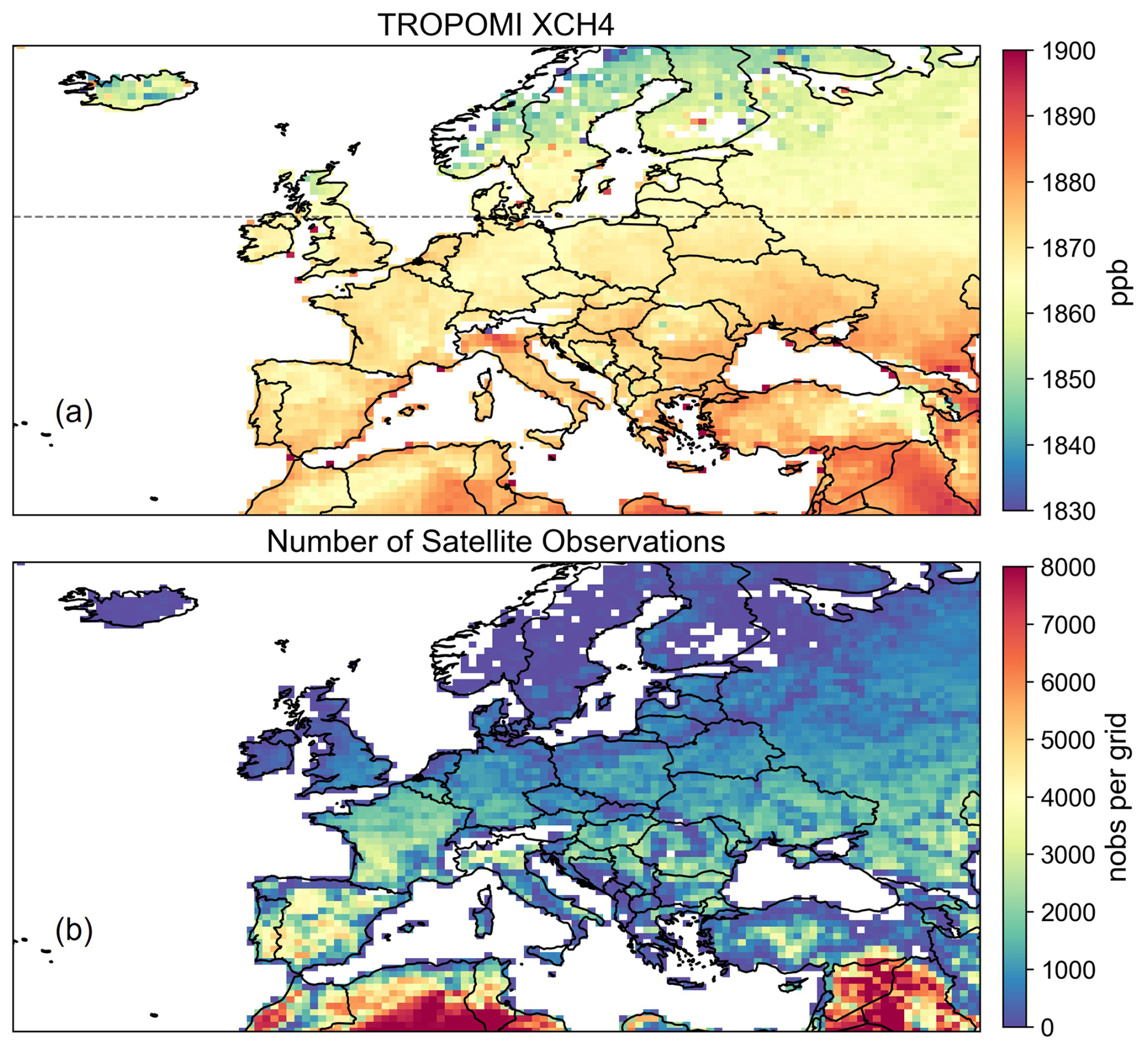
Figure 1 TROPOMI satellite observations. (a) Spatial distribution of annual average TROPOMI methane column-averaged mixing ratios over Europe from 2019 to 2023. The black dashed line marks the northern limit (55° N) of the satellite observations used in the inversion. Satellite observations poleward of 55° N are excluded owing to snow cover, unfavorable illumination, and increased stratospheric model uncertainty. (b) Spatial distribution of the number of TROPOMI observations from 2019 to 2023. Data are plotted in a 0.5° × 0.625° grid.

2.2 Surface observations

We also use ground-based methane observations from the Integrated Carbon Observation System (ICOS) network across Europe (https://www.icos-cp.eu/data-products/atmosphere-release, last access: 13 October 2026; ICOS RI et al., 2025). We use hourly dry-air methane mole fraction observations from 28 ICOS atmospheric stations (Table S3), filtered for valid measurements (Flag = “O”). For 2019–2023, we compute daily daytime averages using data between 10:00 and 16:00 local time, which generally represent well-mixed boundary layer conditions. High-altitude mountain stations are excluded from the inversion due to representativeness issues associated with daytime observations at these sites (Ioannidis et al., 2026; Steiner et al., 2024) (Table S3).

Figure 2 shows the spatial distribution of the ICOS stations used in our analysis, alongside their 2019–2023 mean methane concentrations. The surface sites are predominantly clustered in western Europe, particularly in Germany, the Netherlands, and northern France (Fig. 2). Additional sites are located in the UK and Northern Europe (Fig. 2). These regions correspond to areas with sparse satellite data coverage (Fig. 1), underscoring the strong complementarity between satellite and surface observations for constraining methane emissions. Furthermore, the surface measurements reveal elevated methane concentrations in the Netherlands, northern Italy, and northwestern Germany (Fig. 2), generally consistent with the hotspots of elevated XCH₄ in satellite observations (Fig. 1).

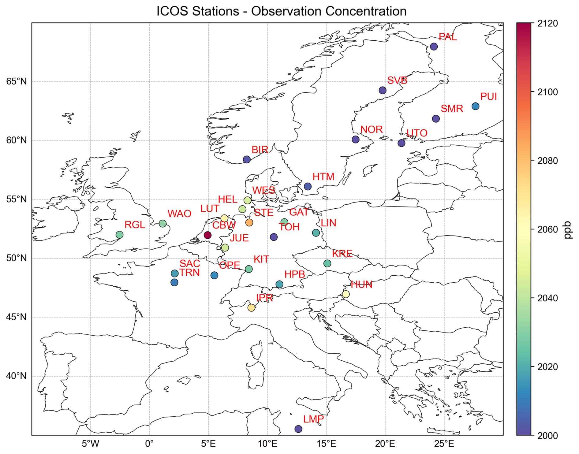
Figure 2 ICOS surface observations. Site locations and their 2019–2023 daytime average concentrations are shown.

2.3 Prior emissions

Figure 3 shows the spatial distribution of prior emissions by sector in the inversion domain. Table S1 tabulates national totals and their sectoral breakdown. Prior anthropogenic emissions (including agriculture, fossil fuel, and waste) are taken from the Emissions Database for Global Atmospheric Research (EDGAR) v8 global emission inventory for 2019–2022 (Crippa et al., 2023). Since 2023 data are not available in EDGAR v8, the 2022 emissions are used for 2023. Prior natural emissions are compiled from multiple datasets: wetland emissions from the ensemble mean of WetCHARTs version 1.0 (Bloom et al., 2017), biomass burning emissions from the Quick Fire Emissions Dataset version 2 (QFED2), termite emissions from Fung et al. (1991), and geological methane emissions based on (Etiope, 2015; Kvenvolden and Rogers, 2005) compiled by Maasakkers et al. (2019). Prior wetland emissions are prescribed at a monthly temporal resolution, and biomass-burning emissions at a daily resolution. Freshwater (rivers and lakes) methane sources (Rocher-Ros et al., 2023; Weber et al., 2019) are not explicitly represented in the prior emissions, considering potential double counting with the wetland inventory (Saunois et al., 2020). Details of the prior emission inventories are provided in Table S2.

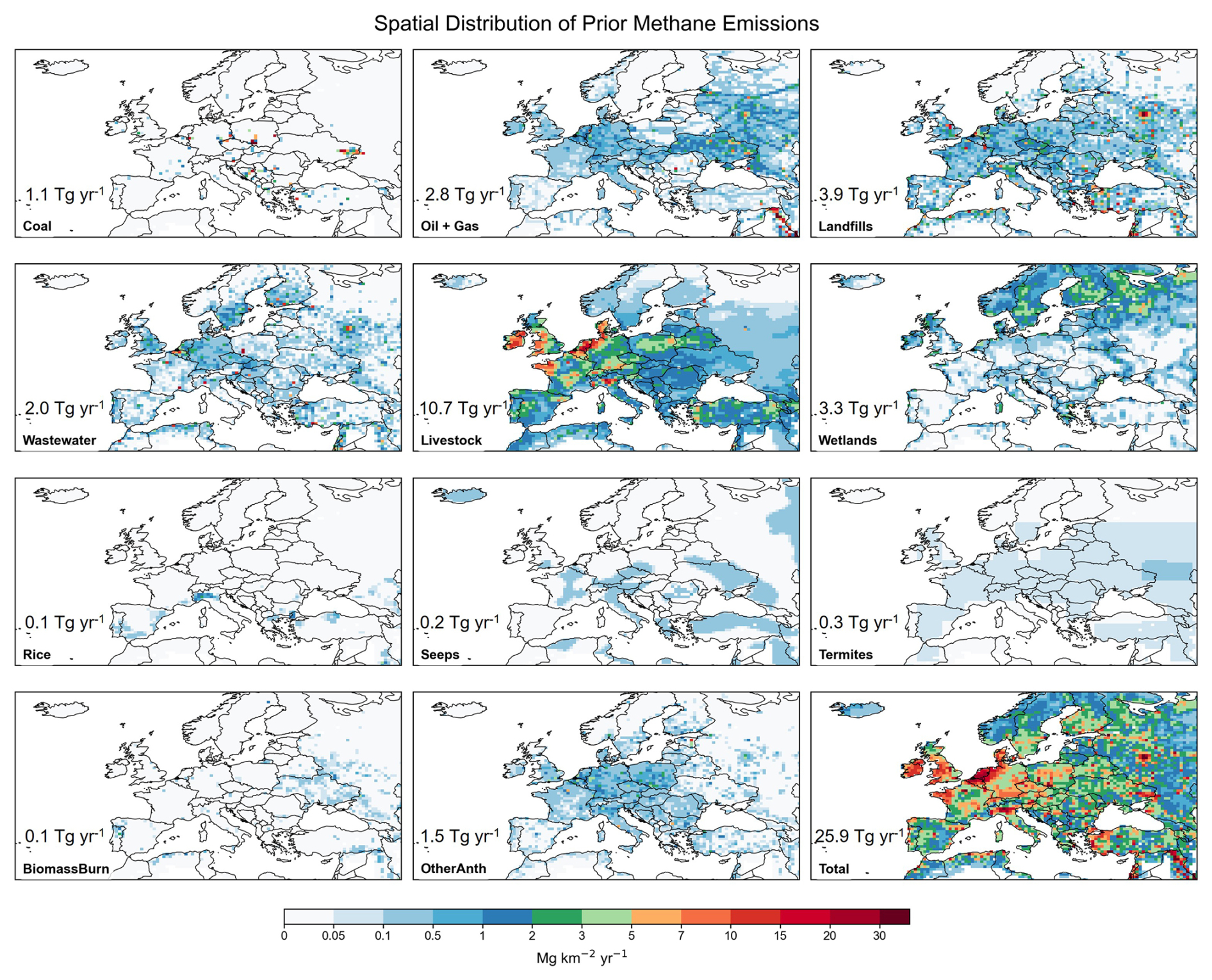
Figure 3 Spatial distributions of prior methane emissions by sector in 2019 over the study domain. The first eleven panels show the spatial distributions of individual methane emission sectors, while the last panel presents the summed methane emissions from all sectors. The values annotated in each panel represent the corresponding total emissions over Europe. Oil and Gas emissions are combined into one panel. OtherAnth denotes the remaining anthropogenic emission sectors not shown separately, including industry, transport, residential combustion, chemical production, iron and steel production, and other minor anthropogenic sources.

These prior emission inventories yield a total methane emission of 25.9 Tg yr⁻¹ for the European countries in 2019, which is mainly from anthropogenic sources (22.0 Tg yr⁻¹). The largest anthropogenic sector in Europe is livestock, distributed primarily in France, Germany, the Netherlands, and the UK (Fig. 3). By contrast, rice cultivation is a minor agricultural source, mainly located in northern Italy (Fig. 3). Oil and natural gas production are concentrated in the North Sea, while coal production is in eastern Europe such as Poland (Fig. 3). The waste sector, including wastewater and landfills, is typically associated with population-dense urban centers (Fig. 3). Natural sources are dominated by northern high-latitude wetlands (Fig. 3). The prior emission inventories indicate a steady decline in anthropogenic methane emissions from the European countries by 0.2 Tg yr⁻² (0.9 % yr⁻¹). The decrease is mainly driven by the waste sector in western Europe, the oil and gas sector in the North Sea, and the coal sector in Ukraine.

2.4 Forward model simulations

We employ the nested version of the GEOS-Chem 12.9.3 chemical transport model (https://zenodo.org/records/3974569, last access: 13 October 2026) as the forward model for the inversion, which relates atmospheric concentrations to surface emissions. The simulation has a horizontal resolution of 0.5° × 0.625° over the European domain (30–70° N, −30–50° E) with 47 vertical layers, and is driven by MERRA-2 reanalysis meteorology from the NASA Global Modeling and Assimilation Office (GMAO) (Gelaro et al., 2017). The atmospheric oxidation of methane is simulated using archived monthly OH, Cl, and stratospheric loss fields (Wecht et al., 2014).

The initial and 3 h dynamic boundary conditions for the regional simulation are taken from a 4° × 5° global GEOS-Chem simulation driven by methane emissions optimized in a global inversion (Ciais et al., 2026). We then quantify and correct residual systematic regional biases in the boundary condition, using satellite and surface observations from background grid cells near the western and northern boundaries, which are the primary inflow pathways into the European domain (Fig. S2). The derived correction, 12 ppb for the western boundary and 30 ppb for the northern boundary (Fig. S2), is applied uniformly to the entire tropospheric vertical profile at both boundaries. This correction is supported by improved agreement with independent IAGOS-CARIBIC aircraft observations (https://www.caribic-atmospheric.com/Data.php, last access: 29 July 2026) in the European free troposphere, reducing the mean bias from 14.1 to 2.9 ppb (Fig. 4). Free tropospheric methane concentrations are largely governed by boundary conditions rather than local surface emissions, making these aircraft data suitable for evaluating boundary conditions. This argument is further supported by the minimal change in simulated free tropospheric methane concentrations between the prior and posterior simulations (Fig. 4).

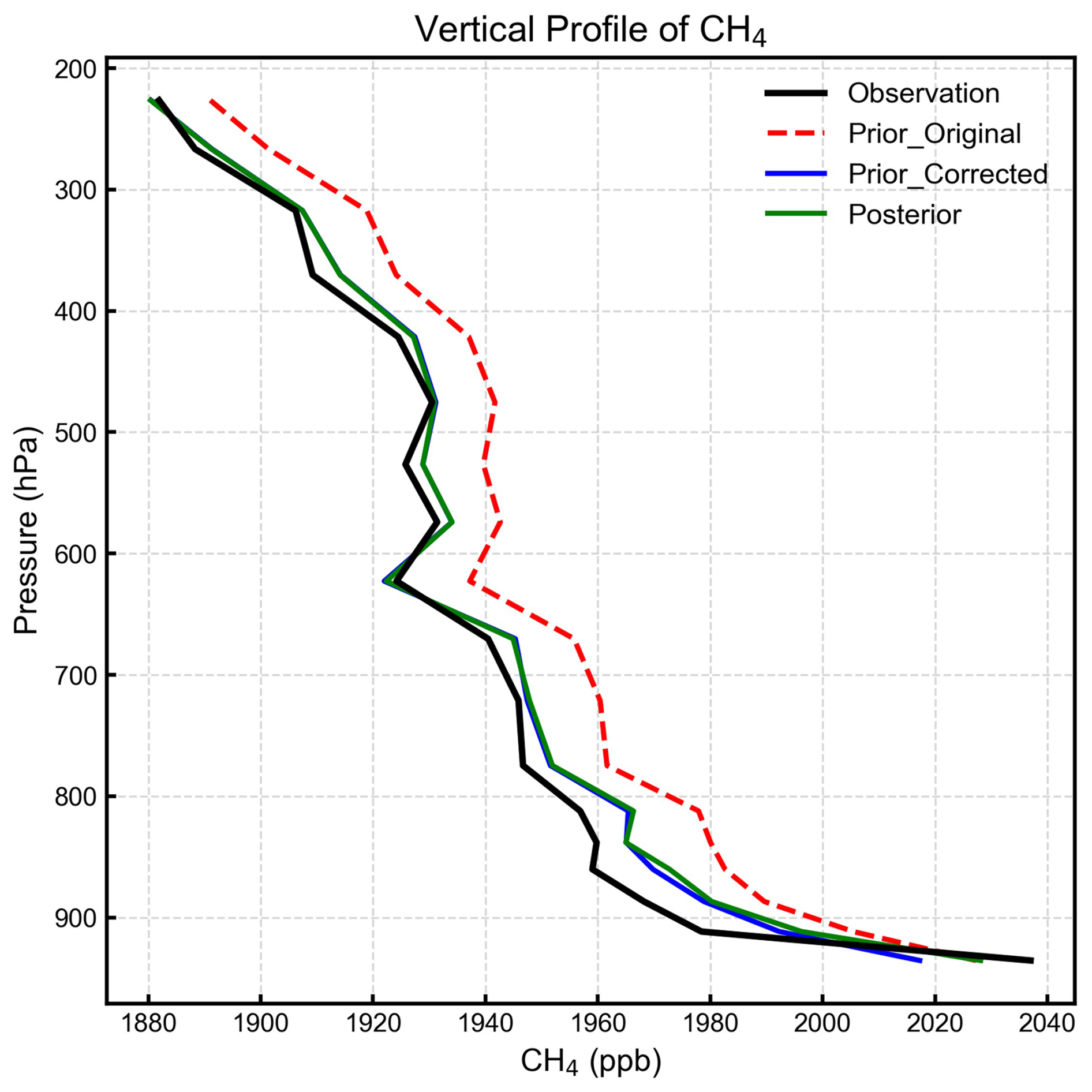
Figure 4 Comparison of simulated vertical profiles of methane mixing ratios with independent aircraft measurements from the IAGOS-CARIBIC project. The black line represents average aircraft observations (Observation), the red line represents the prior simulation with unadjusted boundary conditions (Prior_Original), the blue line represents the prior simulation with bias-corrected boundary conditions (Prior_Corrected), and the green line represents the posterior simulation (Posterior). For this study, we selected methane measurements within the European region and confined to the troposphere, spanning from 2019 to March 2020, resulting in a total of 8418 observations.

To compare with satellite or surface observations, we sample methane fields simulated by GEOS-Chem at the location and time of individual observations. For surface data, we compute daily daytime averages (10:00–16:00 local time) as applied to the hourly in situ measurements. For satellite data, we compute column-averaged methane mole fractions by accounting for the instrument's vertical sensitivity and the prior methane vertical profile.

2.5 Inversion procedure

We perform analytical Bayesian inversion following Zhang et al. (2022) to estimate methane emissions from Europe. The inversion, performed separately for each calendar year, optimizes a state vector x consisting of annual methane emissions from 824 spatial clusters across the study domain (819 clusters for land and 5 clusters for the North Sea, shown in Fig. 5d). We first assign the number of clusters to each country based on the country area and prior methane emissions, and then generate spatial clusters using the Gaussian Mixture Model (GMM) (Turner and Jacob, 2015) for each country.

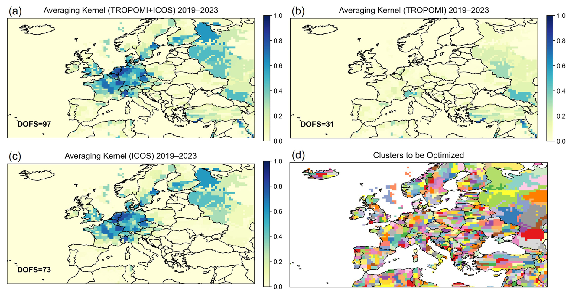
Figure 5 Five-year mean spatial distribution of averaging-kernel sensitivities derived from the annual inversions for 2019–2023 using (a) satellite and surface (TROPOMI+ICOS) observations, (b) only satellite (TROPOMI) observations, and (c) only surface (ICOS) observations. DOFSs of these inversions for the entire domain are inset. Panel (d) shows the spatial clusters defining the inversion state space, constructed using a Gaussian Mixture Model (GMM). Note that, the relatively high ICOS-only sensitivities over western Russia reflect indirect transport constraints on large optimization clusters rather than direct local observations.

The optimal solution of the state vector x is solved by minimizing a Bayesian cost function that incorporates both prior knowledge and observational constraints (Brasseur and Jacob, 2017):

$$\begin{array}{}\text{(1)}& \begin{array}{rl}J\left(\mathit{x}\right)& ={\left(\mathit{x}-{\mathit{x}}_a\right)}^{\mathrm{T}}{\mathbf{S}}_a^{-\mathrm{1}}\left(\mathit{x}-{\mathit{x}}_a\right)\\ & +{\left(\mathit{y}-F\left(\mathit{x}\right)\right)}^{\mathrm{T}}{\mathbf{S}}_{\mathrm{O}}^{-\mathrm{1}}\left(\mathit{y}-F\left(\mathit{x}\right)\right)\end{array}\end{array}$$

where y is the observation vector that contains satellite and surface observations, x_a denotes the prior estimate for x, S_a is the prior error covariance matrix, S_O is the observing system error covariance matrix, and F(x) represents the forward simulation by GEOS-Chem. We treat S_a as a diagonal matrix with a 50 % relative uncertainty assigned to annual methane emissions of each spatial cluster to be optimized. The observing system error covariance matrix, which accounts for random instrument and forward model errors, is represented by a diagonal approximation (S_O) of the full matrix (S_O′), which is populated with the error variance of individual observations (on average ∼ 12 ppb for satellite and ∼ 40 ppb for surface) along with spatial and temporal correlations between observations (spatial correlation length of 500 km for satellite and temporal correlation length of 2 d for both satellite and surface) derived from the error residual method (Figs. S3, S4 and Table S4). The diagonal approximation (S_O) of S_O′ is solved following the method of Zhang et al. (2022) and Liang et al. (2023) (see details in Sect. S1). Additionally, we perform sensitivity inversions in which the observation vector (y) contains either satellite data alone or surface data alone. This allows us to examine the consistency between the two platforms and quantify the observational constraints provided by each.

Minimizing J(x) yields the analytic solutions for the optimal estimate,

$$\begin{array}{}\text{(2)}& \widehat{\mathit{x}}={\mathit{x}}_a+{\left({\mathbf{K}}^{\mathrm{T}}{\mathbf{S}}_{\mathrm{O}}^{-\mathrm{1}}\mathbf{K}+{\mathbf{S}}_a^{-\mathrm{1}}\right)}^{-\mathrm{1}}{\mathbf{K}}^{\mathrm{T}}{\mathbf{S}}_{\mathrm{O}}^{-\mathrm{1}}\left(\mathit{y}-F\left({\mathit{x}}_a\right)\right)\end{array}$$

Linearizing the forward model $F\left(\mathit{x}\right)=\mathbf{K}\mathit{x}+\mathit{c}$ (c is a constant vector) results in the Jacobian matrix K, which represents the sensitivity of methane concentrations to emissions ($\partial \mathit{y}/\partial \mathit{x}$). The matrix K is explicitly constructed by performing GEOS-Chem model simulations with individual state vector elements perturbed.

The analytical solution also yields solutions for the posterior error covariance matrix and the averaging kernel matrix:

$$\begin{array}{}\text{(3)}& {\displaystyle }\widehat{\mathbf{S}}={\left({\mathbf{K}}^{\mathrm{T}}{\mathbf{S}}_{\mathrm{O}}^{-\mathrm{1}}\mathbf{K}+{\mathbf{S}}_a^{-\mathrm{1}}\right)}^{-\mathrm{1}}\text{(4)}& {\displaystyle }\mathbf{A}={\displaystyle \frac{\partial \widehat{\mathit{x}}}{\partial \mathit{x}}}=\mathbf{I}-\widehat{\mathbf{S}}{\mathbf{S}}_a^{-\mathrm{1}}\end{array}$$

The posterior error covariance matrix ($\widehat{\mathbf{S}}$) provides a quantitative measure of the uncertainty associated with the optimized emissions. The averaging kernel matrix (A) describes the sensitivity of the posterior estimate to the true state, with values ranging from 0 (no constraint) to 1 (fully constrained by observations). The trace of matrix A, known as the degrees of freedom for signal (DOFS), quantifies the number of independent pieces of information that are effectively constrained by the observing system. The analysis of A and associated DOFS allows us to quantify the information content provided by satellite and surface observations.

The optimized emissions ($\widehat{\mathit{x}}$) can be projected back onto the spatial grid to obtain the distribution of methane fluxes. To assess emissions at the national scale, we further aggregate the posterior fluxes by country. This is achieved by constructing a transformation matrix W that maps the gridded flux vector ($\widehat{\mathit{x}}$) to national totals. The national-level posterior flux (${\widehat{\mathit{x}}}_{\mathrm{country}}$), posterior error covariance matrix (${\widehat{\mathbf{S}}}_{\mathrm{country}}$), and averaging kernel matrix (A_country) can be calculated as:

$$\begin{array}{}\text{(5)}& {\displaystyle }{\widehat{\mathit{x}}}_{\mathrm{country}}=\mathbf{W}\widehat{\mathit{x}}\text{(6)}& {\displaystyle }{\widehat{\mathbf{S}}}_{\mathrm{country}}=\mathbf{W}\widehat{\mathbf{S}}{\mathbf{W}}^{\mathrm{T}}\text{(7)}& {\displaystyle }{\mathbf{A}}_{\mathrm{country}}=\mathbf{I}-\mathbf{W}\widehat{\mathbf{S}}{\mathbf{W}}^{\mathrm{T}}{\left({\mathbf{WS}}_a{\mathbf{W}}^{\mathrm{T}}\right)}^{-\mathrm{1}}\end{array}$$

Prior uncertainties for national estimates are aggregated following the same approach as in Eq. (6), but with the prior error covariance matrix S_a substituted in the right-hand term.

We derive sectoral methane emissions by partitioning posterior emissions in each grid cell according to prior sectoral fractions. This approach is more effective where major sectors are spatially segregated, but may misattribute emissions in regions with significant sectoral overlap (Lu et al., 2022). Although sectoral information is not directly constrained by methane observations, the sectoral estimates offer useful interpretive insights.

2.6 Inversion evaluation

The joint inversion of TROPOMI and ICOS data improves the fit to both satellite and surface observations, with reduction of root-mean-square errors (RMSE) by 7.95 ppb for ICOS and by 0.84 ppb for TROPOMI (Fig. S6). Cross verification further shows that each single-dataset inversion also improves the fit to the other dataset. The TROPOMI-only inversion reduces RMSE against ICOS by 1.31 ppb, while the ICOS-only inversion reduces RMSE against TROPOMI by 0.09 ppb (Fig. S7). Although these improvements are relatively small, they confirm broad consistency between the two datasets. The posterior simulation also reproduces the observed seasonal variability in methane concentrations (Fig. S5), indicating no substantial seasonal biases in the annually optimized emissions. We further evaluate the inversion against independent ground-based column observations from the TCCON network (https://tccondata.org/, last access: 29 July 2026). Compared to the prior simulation, the posterior simulation reduces the RMSE by about 1 ppb at five of the seven TCCON sites in Europe. These sites with improved agreement are located mostly in western Europe (mainly Germany and France) where the observation constraints are strong, while the other two sites are in the UK and Cyprus where observation constraints are weak (see discussion in Sect. 3). In addition, we also evaluate the inversion against near-surface vertical gradients derived from independent IAGOS-CARIBIC aircraft observations (Fig. S8). Since most vertical profile observations are only available over Germany, where IAGOS-CARIBIC aircraft take off or land, this evaluation only provides information at local to regional scales. Compared to the prior simulation, the posterior simulation generates a sharper concentration gradient between the lower free troposphere and the surface, bringing the simulated profiles into closer agreement with the aircraft observations. The enhanced near-surface gradient reflects the upward adjustment of methane emissions over Germany inferred by the inversion (see Sect. 5.1). Overall, independent observation data remain spatially limited, preventing a systematic assessment of the inversion across the entire European domain.

3 Observational constraints by satellite and surface observations

Figure 5a presents the spatial distribution of averaging kernel sensitivities across the inversion domain, derived from a joint inversion of satellite and surface observations. The averaging kernel sensitivities, defined as the diagonal elements of the averaging kernel matrix (see Eq. 4), quantify the degree to which the inversion system can independently constrain methane emissions at a given location. A value of zero indicates no observational constraint, while a value of one represents full constraint. The results reveal that methane emissions are not uniformly constrained across the inversion domain. Stronger constraints are observed over central and western Europe (primarily Germany and the Benelux states), whereas eastern and northern regions remain comparatively weakly constrained (Fig. 5a). This joint inversion achieves degrees of freedom for signal (DOFS; the sum of the diagonal elements of the averaging kernel matrix, representing the number of independently constrained pieces of information) of 97 for the entire domain, 75 for the European countries, and 64 for the EU27 countries, with DOFS for individual countries tabulated in Table S1.

To evaluate the respective contributions of satellite and surface observations, we also derived averaging kernel sensitivities from inversions using either satellite or surface observations alone (Fig. 5b and c; Table S1). The satellite-only inversion yields a DOFS of 31 for the entire domain, 13 for the European countries, and 11 for the EU27 countries. In contrast, the surface-only inversion yields a DOFS of 73 for the entire domain, 69 for the European countries, and 59 for EU27, respectively, indicating that surface observations provide most of the observational constraints across Europe. The constraints from surface observations are particularly strong over central and western Europe, where ICOS station density is high, but remain limited over the Iberian Peninsula, southern Italy, and eastern Europe (e.g., Poland and Ukraine), regions with almost no surface data coverage. Satellite data offer little additional information over central and western Europe but provide valuable supplementary constraints over the Iberian Peninsula, eastern Europe, western Russia, and adjacent regions such as Turkey and North Africa. In northern Italy, both satellite and surface observations contribute to constraining emissions. In summary, while the most effective constraint on European methane emissions comes from the synergistic use of both platforms, the surface network remains the primary driver of the inversion's information content, with satellite observations playing a secondary role that becomes useful in areas poorly covered by ground-based networks.

4 2019–2023 European methane budget

Figure 6 presents the annual anthropogenic methane emissions aggregated across Europe (excluding Russia and other non-European regions in the inversion domain) for 2019–2023. The inversion yields a 2019–2023 mean total methane emission of 25.7 Tg yr⁻¹ over Europe, including 22.5 Tg yr⁻¹ from anthropogenic sources and 3.2 Tg yr⁻¹ from natural sources. Livestock is the largest anthropogenic source at 11.6 Tg yr⁻¹, followed by landfills (3.9 Tg yr⁻¹), natural gas (2.1 Tg yr⁻¹), wastewater (1.9 Tg yr⁻¹), coal (0.92 Tg yr⁻¹), and oil (0.36 Tg yr⁻¹) (Fig. 7). The total anthropogenic emissions are on average 1.0 Tg yr⁻¹ higher than the prior estimate. The largest sectoral adjustment is for livestock, where emissions are increased by about 1.0 Tg yr⁻¹ (10 %) (Fig. 7). For wetland emissions, the largest natural source, the inversion reduces the mean estimate from 3.3 to 2.6 Tg yr⁻¹(Fig. 7).

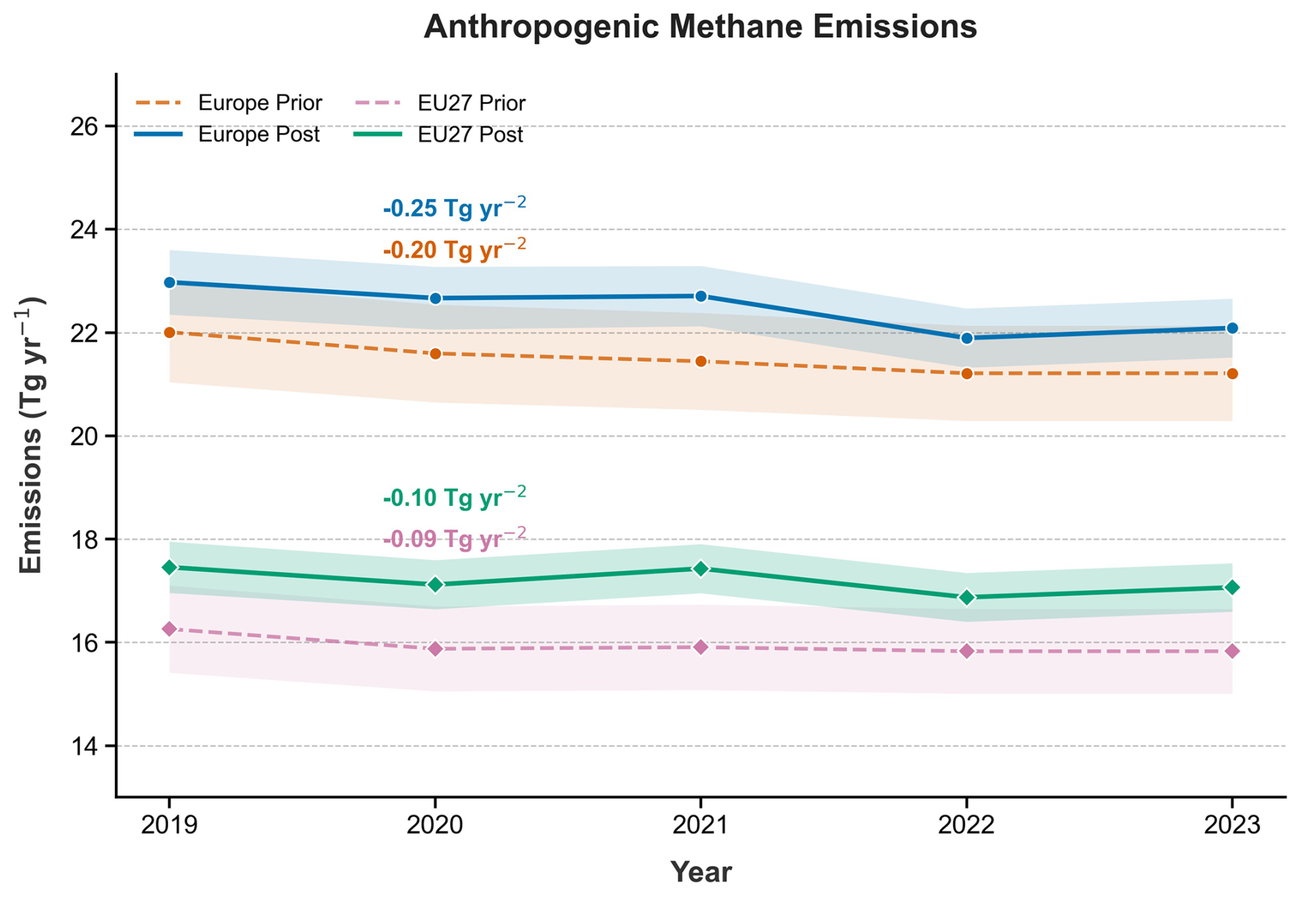
Figure 6 Time series of prior and posterior anthropogenic methane emissions from Europe and EU27. Color shadings represent one standard deviation uncertainties of the prior and posterior estimates. Values of linear trends are inset.

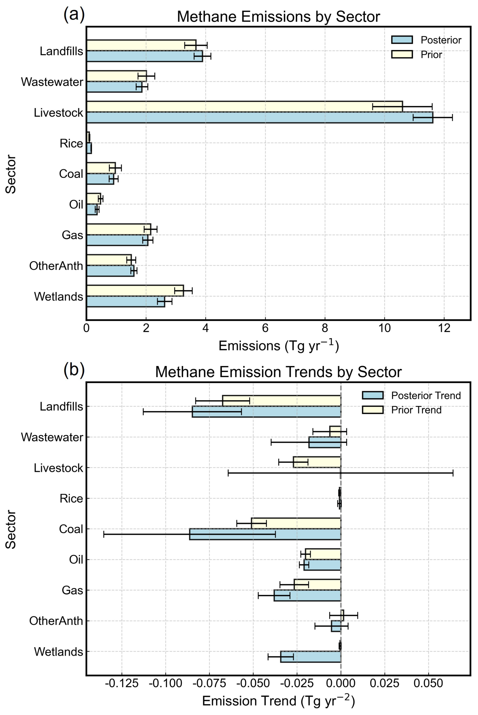
Figure 7 Mean methane emissions from major anthropogenic sectors and wetlands in Europe during 2019–2023 (a), and their emission trends during 2019–2023 (b). Yellow bars represent prior estimates and blue bars represent posterior estimates. Geological seepage, biomass-burning, and termite emissions are not shown separately because their contributions are small relative to the displayed sectors. Error bars denote one standard deviation uncertainties of the prior and posterior estimates.

For the EU27 countries, the inversion yields a posterior anthropogenic methane emission estimate of 17.2 Tg yr⁻¹ over 2019–2023, which is 1.3 Tg yr⁻¹ (8.0 %) higher than the prior estimate of 15.9 Tg yr⁻¹, indicating an underestimation by the prior inventory. The magnitude of this adjustment is comparable to that inferred for the whole of Europe, suggesting that the revision by the inversion is primarily due to EU member states.

Both prior and posterior estimates show a significant negative trend in total anthropogenic emissions at the continental scale (prior: −0.20 Tg yr⁻²; p=0.015; posterior: −0.25 Tg yr⁻²; p=0.046) (Fig. 6), indicating that the observational data support an overall decline in European methane emissions. Linear trends were estimated using ordinary least-squares regression and considered significant at p<0.05. The decrease is primarily driven by reductions in landfill (posterior: −0.08 ± 0.03 Tg yr⁻²), coal mining (−0.09 ± 0.05 Tg yr⁻²), and natural gas (−0.04 ± 0.01 Tg yr⁻²) emissions. In contrast, trends for livestock (−0.0002 ± 0.06 Tg yr⁻²) and wastewater (−0.02  ±  0.02 Tg yr⁻²) are insignificant given the uncertainties. We also find a decrease in wetland emissions of −0.03 ± 0.01 Tg yr⁻² over the study period. For the EU27, anthropogenic emissions also decreased (prior: −0.09 Tg yr⁻², p=0.11; posterior: −0.10 Tg yr⁻², p=0.23), although the trends are not statistically significant.

5 2019–2023 mean methane emissions

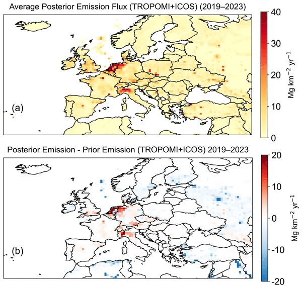
Figure 8 presents the spatial distribution of posterior methane emissions averaged over the period from 2019 to 2023 and the inversion's adjustments relative to prior emissions. Figure 9 summarizes prior and posterior estimates of anthropogenic emissions from the major emitters in Europe, in comparison with their UNFCCC-reported emissions for 2023 (https://unfccc.int/ghg-inventories-annex-i-parties/2026, last access: 29 July 2026) and estimates from previous inversion studies. Inversion results for all European countries during 2019–2023 are archived in Table S1. Overall, the posterior estimate yields a spatial distribution of methane emissions across Europe that is broadly consistent with prior knowledge (Fig. 8). For instance, the prior and posterior show that methane emissions concentrate in central and western Europe, reflecting intensive agriculture, waste treatment, and fossil fuel production (Fig. 3). Meanwhile, the inversion reveals substantial regional adjustments to the prior estimates. Notable upward revisions occur in regions with intensive agriculture and waste sources, such as the Netherlands, northwestern Germany, and northern Italy, as well as in urban centers across France, Spain, and the southern United Kingdom. In contrast, downward adjustments are found in offshore oil production regions in the North Sea and in boreal wetland areas (Fig. 8). In the following sections, we discuss these inversion-informed revisions to the 2019–2023 average methane emissions for each region, with 2023 country-level estimates used for comparison with UNFCCC inventories and previous inversion studies.

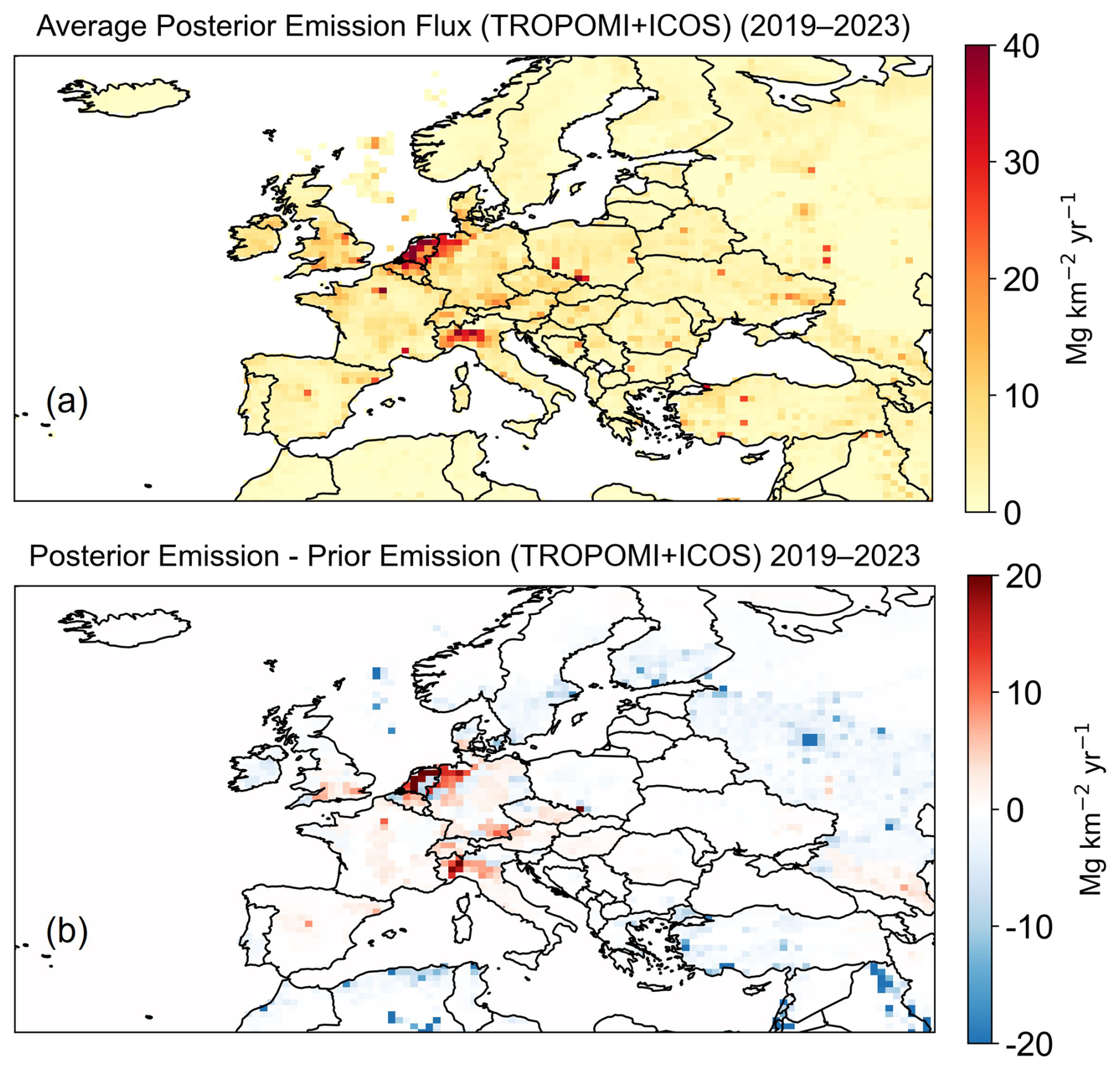
Figure 8 Spatial distributions of 2019–2023 average posterior methane emissions in Europe. (a) Five-year average posterior emissions. (b) Adjustment of methane emissions by the inversion expressed as posterior minus prior.

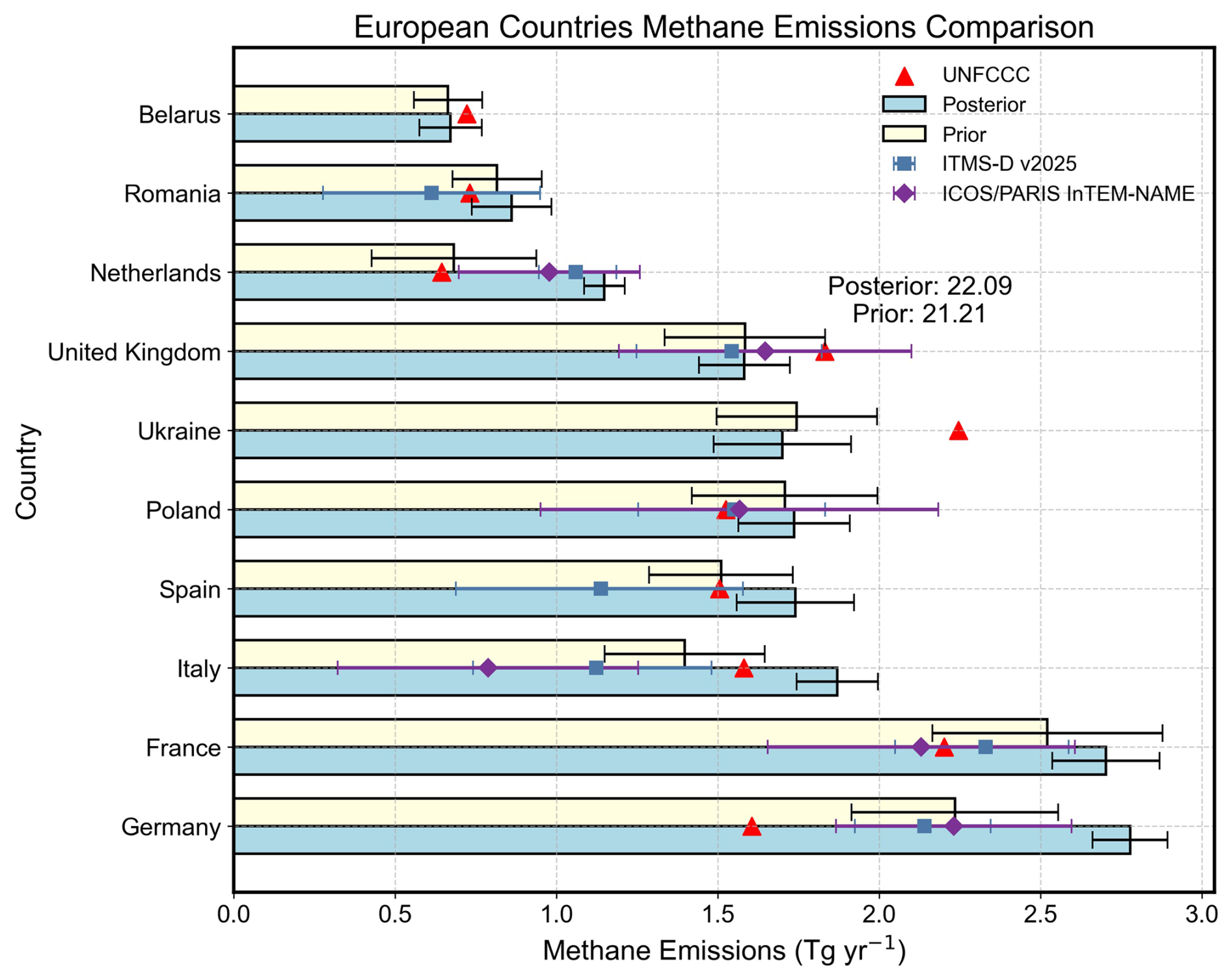
Figure 9 Anthropogenic methane emissions in 2023 for the major European countries with the largest anthropogenic emissions in our inversion domain. Yellow and blue bars represent prior and posterior emissions, respectively. The results are compared with UNFCCC-reported emissions for inventory year 2023 (red triangles), country-level non-natural posterior emissions from ITMS-D v2025 (blue squares), and country-level total posterior methane fluxes from ICOS/PARIS InTEM-NAME (purple diamonds). Error bars for our prior and posterior estimates denote one standard deviation. Error bars for ITMS-D v2025 and ICOS/PARIS InTEM-NAME denote the posterior percentile ranges provided by the respective products.

5.1 Agriculture dominated regions

We find that the inversion upward adjusts prior methane emissions from the Netherlands, northwestern Germany, and northern Italy (Fig. 8). The posterior estimates of anthropogenic emissions for these countries (Germany: 2.78 ± 0.12 Tg yr⁻¹; Netherlands: 1.15 ± 0.06 Tg yr⁻¹; Italy: 1.87 ± 0.13 Tg yr⁻¹) are 25 %–69 % higher than prior estimates (Germany: 2.23 Tg yr⁻¹; Netherlands: 0.68 Tg yr⁻¹; Italy: 1.40 Tg yr⁻¹) and 18 %–80 % higher than official reports to the UNFCCC (Germany: 1.60 Tg yr⁻¹; Netherlands: 0.64 Tg yr⁻¹; Italy: 1.58 Tg yr⁻¹) (Fig. 9). Our posterior estimates are generally comparable in magnitude with the independent country-level estimates from ITMS-D v2025 (Bruch et al., 2026) and ICOS/PARIS InTEM-NAME (Ganesan et al., 2026). The upward adjustments in these regions are derived from both of our sensitivity inversions, using either surface or satellite observations alone (Fig. S10), although the magnitudes of the adjustments differ (e.g., stronger and spatially uneven adjustment inferred by surface-only inversion than satellite-only inversion) due to varying observational constraints (Fig. 5). This general consistency in directions provides additional support that the upward adjustment is robust across different observation platforms in this region.

Based on the relative contribution of each sector in the prior inventory, we attribute most of the upward adjustment in the Netherlands, Germany, and Italy to the agriculture sector (Fig. 10). This finding is consistent with a recent satellite inversion over western and central Europe, which inferred a 17 %–29 % increase in CAMS livestock emissions (Oak et al., 2026). Our attribution to agricultural emissions also aligns with a recent local-scale survey of 51 Dutch dairy farms, which reported average whole-farm methane emissions 27 % higher than Dutch National Inventory estimates, though those local measurements carried substantial uncertainties of their own and may not fully represent national conditions (Chen et al., 2025). By contrast, urban emission measurements in several cities of these countries, including Berlin (Klausner et al., 2020), Groningen, Utrecht, Rotterdam (Tong et al., 2023), and Milan (Cristofanelli et al., 2025), have not shown significant discrepancies from EDGAR or official inventories, suggesting that the regional underestimation inferred by the inversion is unlikely to stem primarily from urban sources. Taken together, these results point to potential systematic biases in national-level livestock emission accounting, even when high-tier methodologies that incorporate detailed activity data on animal diet, milk production, and feed use are employed (Bruch et al., 2025; Steiner et al., 2024).

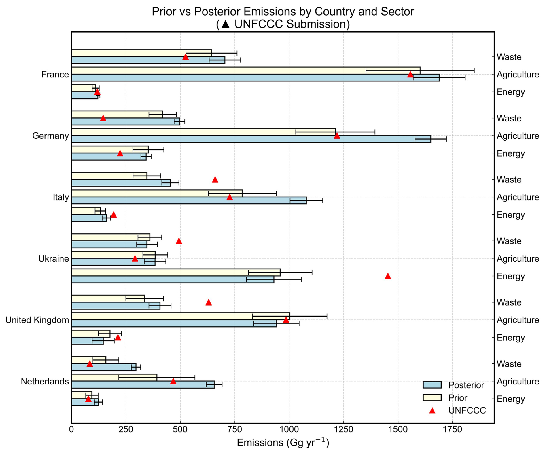
Figure 10 Sector breakdown of national anthropogenic emissions in 2023 for six key countries in Europe. Yellow bars represent prior emissions, blue bars posterior emissions, and red triangles official reports to the UNFCCC as a comparison. Error bars for our prior and posterior estimates denote one standard deviation. Based on the UNFCCC sectors, we group oil, gas, and coal as Energy, livestock and rice as Agriculture, and landfills and wastewater as Waste. IPPU and LULUCF sectors, reported in UNFCCC data, are ignored, as their contributions are minor compared to agriculture, waste, and energy sectors (Fig. 3).

Despite the above evidence, our sectoral attribution is inherently limited in regions with spatial overlap among major sectors or poor prior representation of key sources. Coastal wetland and freshwater emissions, absent from our prior, may partly explain the inferred increase over the Netherlands (Buzacott et al., 2024). Geological emissions introduce major uncertainty in Italy. Etiope et al. (2019) estimated ∼ 2 Tg yr⁻¹ from geological seeps, compared to negligible amounts in our prior (∼ 0.03 Tg yr⁻¹), mirroring large discrepancy in global geological emissions using different approaches (Hmiel et al., 2020; Etiope et al., 2019). This leads to considerable uncertainties in both total emission estimation and sectoral attribution, particularly where agricultural and geological sources are spatially closely located like northern Italy. Given their important implications for distinguishing natural from anthropogenic emissions, these limitations warrant further targeted investigation. Moreover, future inversion studies could leverage observed seasonality (Ioannidis et al., 2026) and sector-specific tracers such as NH₃ (Tang et al., 2025) to enhance the ability to quantify agricultural emissions.

5.2 Fossil fuel production regions

In addition to agriculture- and waste-related sources, the inversion analysis also revises methane emission estimates for several fossil fuel production regions, including the North Sea and southern Poland (Fig. 8). For the North Sea, posterior emissions from offshore oil and gas production are 0.28 Tg yr⁻¹, 53.4 % lower than prior estimates. This contrasts with a ship-based study (Riddick et al., 2019), which found substantial emissions from UK offshore platforms, suggesting existing inventories may underestimate. However, those measurements were limited to a short timeframe and may not reflect the variability across different phases of offshore production. This downward adjustment is mainly informed by surface observations, but both satellite- and surface-only inversions agree on its direction (Fig. S10).

Over southern Poland, the inversion reveals a revised spatial pattern of emissions within the Upper Silesian Coal Basin (Fig. 8), a major production hub accounting for the majority of the EU's hard coal output. Despite this spatial redistribution, the national estimates for anthropogenic emissions remain nearly unchanged at 1.7 Tg yr⁻¹, whereas coal mining emissions increase from 0.40 to 0.47 Tg yr⁻¹ (Fig. 9 and Table S1). The posterior coal-mining estimate is broadly consistent in magnitude with previous multi-scale observational studies conducted in the Upper Silesian Coal Basin, ranging from individual mine shafts to basin-wide assessments (Andersen et al., 2023; Fiehn et al., 2020; Luther et al., 2019, 2022; Tu et al., 2022).

Other major fossil fuel producers in Europe, such as Romania and Ukraine, show only minor emission adjustments in our atmospheric inversion (Figs. 8, 9). This is primarily due to limited capacity of the inversion system to constrain emissions in these regions, as indicated by low observational constraints (DOFS of only 0.75 for Romania and 1.38 for Ukraine). Consequently, while our posterior estimate (0.83 Tg yr⁻¹) aligns more closely with the prior EDGAR inventory, it does not conclusively rule out the plausibility of the significantly different UNFCCC value for Ukraine's oil and gas sector (1.5 Tg yr⁻¹) (Fig. 10). This limitation in observational constraint also explains why our inversion infers the relatively small adjustments for Romania (Fig. 8), though aircraft-based studies reveal that UNFCCC reports underestimate emissions from the country's southern oil fields (Maazallahi et al., 2025; Kuhlmann et al., 2025).

In Northern Europe, including wetland-rich areas (Fig. S11), posterior estimates are generally lower than the prior (Fig. 8), implying a possible overestimation of wetland and/or offshore oil and gas emissions. These regional differences reveal localized hotspots or deficits that are not fully captured in the prior inventory. While the prior emissions reproduce broad spatial patterns reasonably well, they may miss finer-scale spatial heterogeneities. However, because of the limited observational coverage, these high-latitude regions are only weakly constrained by observations, hence large uncertainties remain in observationally deriving fossil fuel and wetland emissions in Northern Europe.

5.3 Urban hotspots

The inversion also indicates moderate upward adjustments for anthropogenic emissions across France, Spain, and the terrestrial part of the United Kingdom (Figs. 8, 9). The adjustments for the UK and France are mainly driven by surface data, whereas the adjustment for Spain is driven mainly by satellite observations (Fig. S10). Posterior emissions are 2.70 ± 0.17 Tg yr⁻¹ for France and 1.74 ± 0.18 Tg yr⁻¹ for Spain, representing increases of approximately 7 % and 15 % relative to their prior estimates, respectively (Fig. 9). For the UK, the posterior anthropogenic emissions (1.58 Tg yr⁻¹) remain nearly unchanged from the prior (Fig. 9), as the increase over land is offset by decreases in offshore oil and gas emissions over the ocean. The satellite-only inversion shows little adjustment over southern UK, suggesting that the inferred increase is mainly constrained by the available surface observations, whereas offshore emissions remain weakly constrained.

Spatially, the inversion reveals concentrated upward adjustments over major urban areas such as Paris, Madrid, and London, in addition to weaker, diffuse adjustments that we attribute to agricultural sources (Fig. 8). Consistent with this finding, recent studies using ground-based (Tu et al., 2022) and satellite-based (Dogniaux et al., 2025) remote sensing have identified landfills as a major, underrepresented methane source in Madrid. Eddy covariance flux measurements in central London also show that urban methane fluxes are substantially underestimated in inventories, with contributions from both biogenic and fossil fuel sources (Helfter et al., 2016). Further attributing urban emissions to biogenic versus fossil fuel sources is challenging within our inversion framework due to spatial overlap. Inclusion of additional atmospheric tracers, such as C₂H₆ and δ¹³CH₄, could enhance source attribution of urban methane emissions (McKain et al., 2015; Ramsden et al., 2022; Zhao et al., 2026; Basu et al., 2022).

6 Methane emission trends during 2019–2023

To identify the potential effects of recent mitigation policies, we also derived five-year (2019–2023) linear trends in methane emissions from the inversion. These trends are generally uncertain at regional and national scales due to the short time series and large inter-annual variability, but they provide a first indication of broad directional trends in Europe's methane emissions. Figure 11 presents the spatial distribution of prior and posterior methane emission trends from 2019 to 2023. The inversion reveals substantial regional differences in emission trends. Positive emission trends are inferred by the inversion in the Netherlands, Belgium, western Germany, northern Italy, western Poland, and the southern United Kingdom, in contrast to near-zero trends in the prior estimate. Conversely, negative emission trends are observed in southern Poland and eastern Ukraine. In Germany, the Netherlands, Belgium, and other parts of central and western Europe, methane trends are spatially heterogeneous, with increasing emissions potentially associated with agricultural sources. However, seasonal variability in fossil fuel and waste treatment sectors may introduce confounding signals that are not fully separable at the current resolution and tracer constraints of our inversion system (Ioannidis et al., 2026). The reductions in southern Poland and eastern Ukraine are attributed to coal-related emission declines (Gajdzik et al., 2024; UNECE, 2024).

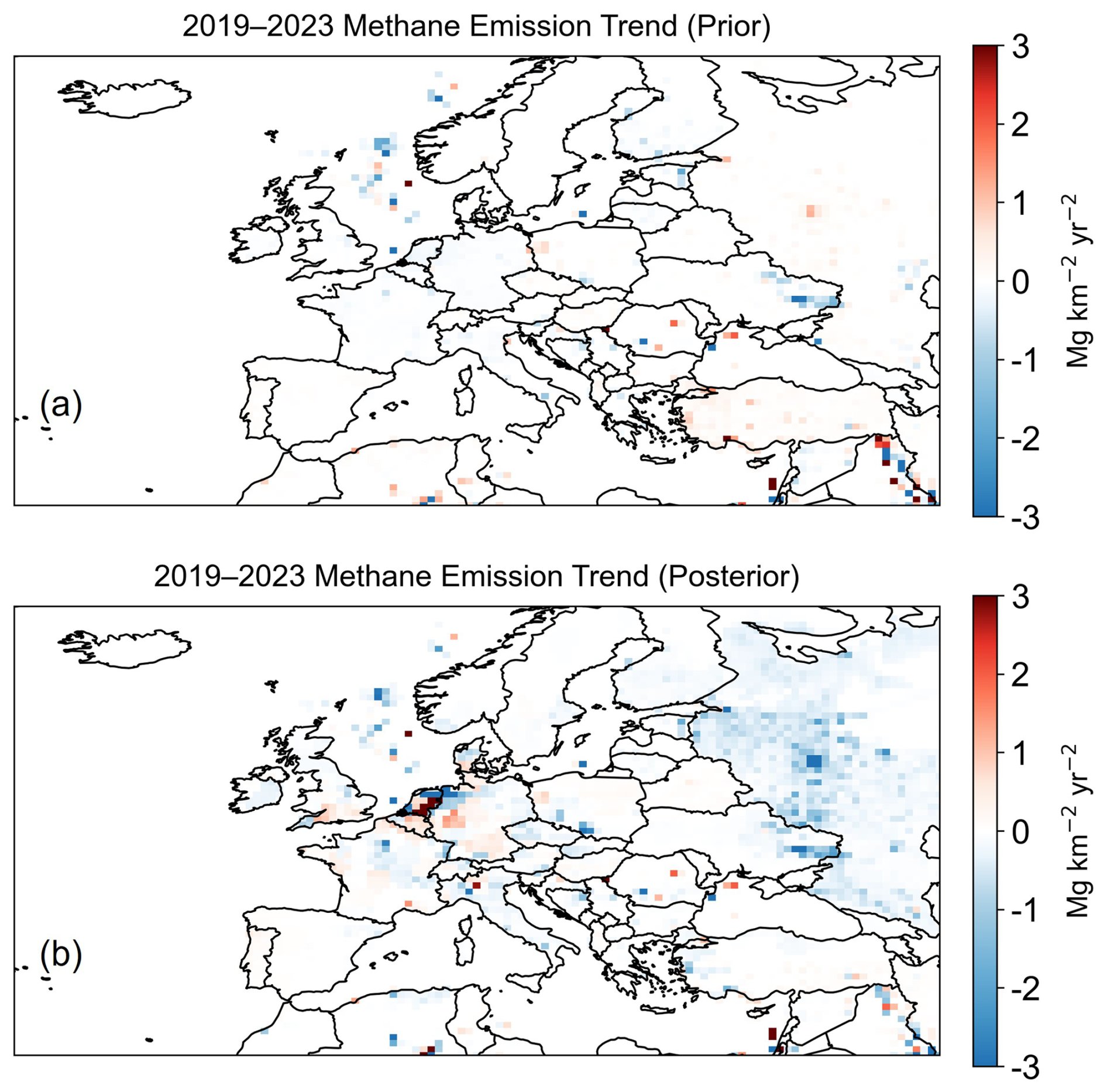
Figure 11 Spatial distributions of methane emission trends in Europe from 2019–2023. Linear trends in (a) prior and (b) posterior methane emissions (TROPOMI+ICOS).

Over the North Sea, both the prior and posterior indicate a modest decreasing trend in methane emissions, with the inversion yielding a trend comparable in magnitude to the prior estimate. This suggests limited adjustment by the inversion in this region, likely reflecting relatively weak observational constraints on offshore emissions. Aircraft-based measurements over the southern North Sea have shown that methane emissions from individual offshore facilities are often underestimated by bottom-up inventories (Pühl et al., 2024), suggesting that such facility-level discrepancies may not be readily detectable as regional-scale emission trends in satellite-based inversions.

Figure 12 presents the 2019–2023 anthropogenic methane emission trends for Europe's major emitting countries. Most countries show consistent trend directions between prior and posterior estimates, with differences generally within posterior uncertainties. France, Italy, Germany, and the United Kingdom exhibit stable or small negative trends in prior and posterior estimates, with no statistically significant differences. Romania and Belarus display weak increases in both datasets, reflecting general agreement. Ukraine shows a consistent decrease but with a stronger posterior trend (−0.09 ± 0.005 Tg yr⁻²) than the prior (−0.05 Tg yr⁻²), suggesting that the prior inventory may underestimate the actual rate of decline. In contrast, the trend directions differ between prior and posterior estimates for countries including the Netherlands and Poland. For instance, the Netherlands shifts from a negative (−0.016 Tg yr⁻²) prior trend to a slightly positive (+0.022 ± 0.01 Tg yr⁻²) posterior trend. For Poland and Spain, the posterior uncertainties encompass the prior values, preventing a definitive conclusion on the trend direction.

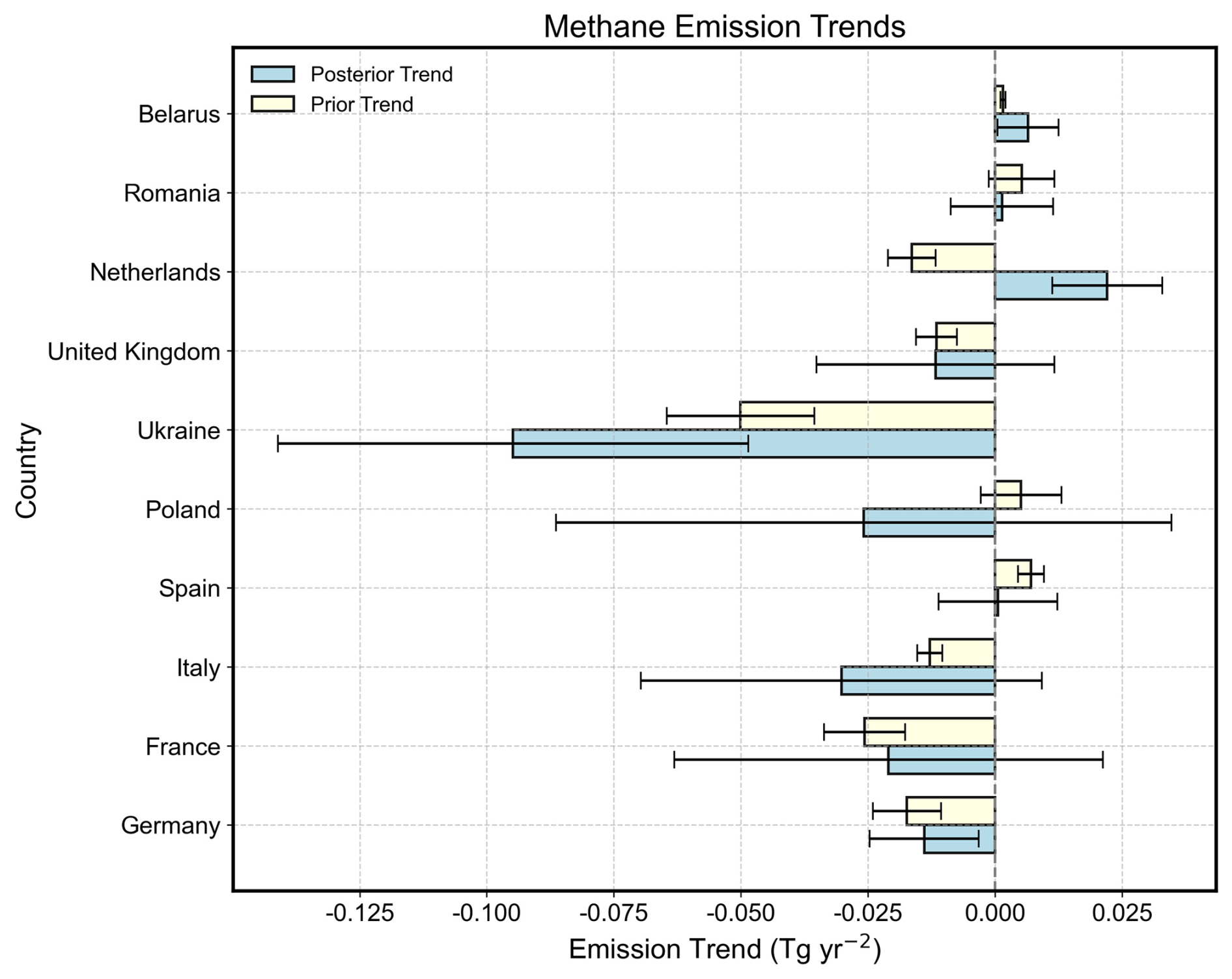
Figure 12 2019–2023 trends in anthropogenic methane emissions for major countries in Europe. Yellow bars represent prior emissions and blue bars posterior emissions. Error bars denote 1 standard deviation uncertainties of prior and posterior emission trends.

7 Conclusions

We quantified European methane emissions from 2019–2023 using a joint inversion of satellite (TROPOMI) and ground-based (ICOS) observations. The inversion achieves a DOFS of 97 across the study domain, with the strongest constraints over central and western Europe. These constraints are driven primarily by surface observations (DOFS =73 in the surface-only inversion). Satellite observations contribute comparatively little additional constraint in regions that are already well covered by surface measurements, but they provide valuable complementary information in areas with sparse surface networks, such as the Iberian Peninsula and eastern Europe (DOFS =31 in the satellite-only inversion).

Our inversion yields an average European methane emission of 25.7 Tg yr⁻¹ for 2019–2023, with anthropogenic sources contributing 22.5 Tg yr⁻¹. Sectorally, livestock is the largest contributor (11.6 Tg yr⁻¹), followed by landfills (3.9 Tg yr⁻¹), wastewater (1.9 Tg yr⁻¹), and fossil fuel activities. The posterior anthropogenic total is 1.0 Tg yr⁻¹ higher than the prior, with the largest upward adjustment (+1.0 Tg yr⁻¹) for livestock emissions, while wetland emission estimates are revised downward. A similar underestimation is found for the EU27. Both prior and posterior estimates show a declining trend in European anthropogenic emissions, primarily driven by reductions in landfills, coal, and natural gas, whereas trends for livestock and wastewater are statistically insignificant.

The inversion reveals substantial adjustment patterns over regions dominated by agricultural and waste sources. Substantial upward adjustments of 25 %–69 % relative to prior methane emissions are inferred by the inversion for Germany, the Netherlands, and Italy. This revision is attributed primarily to underestimated agricultural emissions, a finding consistent with local-scale measurement and recent inversion studies but further targeted studies are needed to corroborate. Moderate upward adjustments of roughly 7 % and 15 % in France and Spain, respectively, are likely driven by underestimated urban sources.

The inversion also revises methane emission estimates for key fossil fuel production regions. Over the North Sea, posterior emissions from offshore oil and gas are 53 % lower than prior estimates. For southern Poland, the inversion refines the spatial pattern of emissions within the Upper Silesian Coal Basin. In contrast, emissions for Romania and Ukraine are only minimally adjusted but this may simply be due to weak observational constraints.

In addition to mean methane emissions, the inversion also reveals trends in methane emissions across Europe from 2019–2023. Notable positive trends are identified in the Netherlands, Belgium, western Germany, northern Italy, western Poland, and the southern United Kingdom, which contrasts with prior bottom-up estimates. Conversely, declines are observed in southern Poland and eastern Ukraine, linked to sector-specific reductions in coal-related emissions. At the national level, while most major emitters show consistent trend directions between prior and posterior estimates, divergences occur for the Netherlands, Poland, and Spain. The posterior trend for the Netherlands changes from −0.016 Tg yr⁻² in the prior to +0.022 ± 0.01 Tg yr⁻², whereas Ukraine exhibits a stronger negative posterior trend (−0.09 ± 0.005 Tg yr⁻²) than the prior estimate (−0.05 Tg yr⁻²).