From prototypical regimes to observed complex dynamics and CO₂ transport in the Amazonian nocturnal boundary layer

We investigated the characteristics of the nocturnal boundary layer (NBL) above and within the Amazon rainforest canopy during the 2022 dry season. We analysed observed NBL dynamics and CO₂ transport from the perspective of the prototypical NBL represented in weather and climate models. To this end, using the CloudRoots-Amazon22 dataset, we characterised the main NBL features and governing processes. We identified NBL height using five methods based on thermal stratification, wind, and turbulent criteria, finding a distinct stable layer above the canopy with an average height between 142–164 m. To examine the drivers of the dynamic NBL evolution, we classified the data into weakly and strongly stable regimes, determined by the interplay between stabilising longwave radiative cooling and destabilising mechanical wind shear. Budget equations for turbulent kinetic energy (TKE), heat, and CO₂ allowed us to quantify the relative contributions of these drivers to transport across the canopy-atmosphere interface. In the weakly stable regime, increased TKE at the canopy top promoted mixing between the within- and above-canopy layers. Conversely, TKE was nearly absent in the strongly stable regime, decoupling the two layers. This decoupling favoured strong thermal stratification above the canopy and well-mixed conditions within the canopy. Our results show that only about 6 % of observed profiles conform to prototypical NBL regimes, emphasising the need to revisit parameterisations to explicitly account for canopy-induced effects and intermittent turbulence. Our observational analysis provides a critical benchmark for improving the representation of NBL dynamics and CO₂ transport in models.

1 Introduction

The Amazon rainforest is considered a crucial terrestrial carbon sink in the global climate system (Science Panel for the Amazon, 2021; IPCC, 2023). However, as a result of climate change and deforestation practices (Costa and Foley, 2000), a decline in its uptake strength has been reported (Brienen et al., 2015; Hubau et al., 2020). Some studies suggest that the Amazon rainforest has already become a net carbon source (Aragão et al., 2014; Hubau et al., 2020; Gatti et al., 2021), while others continue to identify the Amazon as a net carbon sink (Harris et al., 2021). This disagreement largely stems from uncertainties in current modelling estimates, combined with the limited availability of high-quality observations to validate the models used (Rosan et al., 2024). Especially during stratified nighttime conditions, the model representation of key processes in the soil-vegetation-atmosphere continuum remains inaccurate and incompletely evaluated (Cuxart et al., 2006; Svensson et al., 2011; van Stratum and Stevens, 2015; Vilà-Guerau de Arellano et al., 2023).

During the night, net longwave radiative cooling of the canopy top leads to the formation of a stable layer, referred to as the nocturnal boundary layer (NBL) (Mahrt et al., 1979; Garstang and Fitzjarrald, 1999; Mahrt, 1999). This stable stratification has a direct impact on the vertical distribution of CO₂. Because of the stable thermal atmospheric stability above the canopy top, the respired CO₂ is trapped within the canopy and accumulates over time (Mahrt, 1999). The extent to which the in-canopy atmosphere and stable layer aloft interact is governed by the intricate interplay of shear-driven turbulence and buoyancy inhibition at the canopy-atmosphere interface, which can either decrease, maintain or enhance the thermal atmospheric stability (Stull, 1988; Mahrt, 1999).

These canopy-atmosphere interactions are known to be non-stationary in nature, associated with intermittent bursts of turbulence (van de Wiel et al., 2002a, b; Acevedo et al., 2008, 2016; Mahrt, 2011; Santos et al., 2016; Dias-Júnior et al., 2017), and affected by both the characteristics and processes happening within the canopy and the roughness sublayer aloft (de Kauwe et al., 2017). The non-stationarity results from the opposing mechanisms of thermodynamic stratification by longwave radiative cooling and turbulent mixing caused by shear and lead to misrepresentations of the NBL in numerical weather and climate models. In addition, the non-stationarity complicates observations with the eddy covariance (EC) technique, which are limited due to the absence of turbulence and its dependency on height, complicating the validation of nocturnal CO₂ exchange representation (Aubinet, 2008; Nicolini et al., 2018) in numerical weather and climate models.

To represent the interplay of shear and longwave radiative cooling and characterise the different states of the NBL, observational studies often subdivide the available observations from the above-canopy atmosphere into two stability regimes: a strongly stable regime, where turbulence is almost absent and longwave radiative cooling is dominant, and a shear-driven weakly stable regime, where weak turbulent motions limit the stratification (Mahrt, 1998; Oliveira et al., 2013, 2018). In numerical weather and climate models, these regimes are typically represented by prototypical NBL vertical profiles (Edwards et al., 2020) and a simple bulk description of the canopy layer (Boussetta et al., 2013). These prototypical NBL vertical profiles represent the “textbook” profiles described, among others, by Mahrt et al. (1979) and Stull (1988). These prototypical vertical profiles are based on homogeneous, single-layer surfaces and therefore do not account for the multilayer structure of forest canopies (Bonan et al., 2021). Consequently, these parameterisations coarsely describe the canopy-atmosphere interactions, and it is questionable whether these prototypical profiles correctly represent the variability observed in the CO₂ and heat exchange at the Amazonian atmosphere-canopy interface.

To this end, we analyse the comprehensive in-canopy and above-canopy observations from the CloudRoots-Amazon22 field campaign (Vilà-Guerau de Arellano et al., 2024) to perform an in-depth characterisation of the NBL. The analysis is carried out from the perspective of evaluating how the observations follow the two regimes as typically represented in weather and climate models. The final outcome is an in-depth characterisation and quantification of the NBL in the Amazon during the dry season.

2 Methods

The methods consist of four sections. In the first, we introduce the observational dataset acquired during the CloudRoots-Amazon22 field campaign. In the second, we describe the five criteria used to estimate the NBL height (h_NBL). In the third, we describe the method used to assess the stability of the Amazonian NBL within and above the canopy. In the fourth section, we define our methodology to select strongly and weakly stable NBL regimes from the observational dataset, based on six strict criteria. These criteria keep our regimes consistent with the prototypical NBL model representation and allow us to assess how well the prototypical representation captures night-time variations in the dense Amazon rainforest. Additionally, we also describe the governing equations of turbulent kinetic energy (TKE), heat, and CO₂, which we examined to further disentangle the different mechanisms at play during strongly and weakly stable NBL regimes.

2.1 CloudRoots-Amazon22 campaign

Observations of the CloudRoots-Amazon22 campaign were collected at the Amazon Tall Tower Observatory (ATTO) site between 8–21 August 2022, during the Amazonian dry season. The campaign added detailed cloud- and leaf-level observations (Vilà-Guerau de Arellano et al., 2024) to the continuous, high-quality tower flux and concentration measurements (Andreae et al., 2015; van Asperen et al., 2023). For this study specifically, observations were collected from both the 325 m ATTO tall tower (−2.1448° N, −59.0008° E) and the shorter 81 m Instant tower (−2.1468° N, −59.0068° E), which are 670 m apart (Dias-Júnior et al., 2019). We only made use of the observations during the nocturnal period, which we defined as the period between sunset (18:00 LT) and sunrise (06:00 LT), where LT, local time, is UTC-4. Additionally, we excluded the final two days of the campaign (20 and 21 August) because of multiple unavailable variables, including longwave radiative and CO₂ flux observations.

Sensors on the towers are placed at 14 height levels between the two towers, continuously monitoring atmospheric variables, trace gases, and turbulent fluxes (Table 1). The turbulent fluxes were calculated over 30 min intervals and corrected for outliers, temporal trends, double rotation of the wind field, time lags, spectral losses, crosswind effects, and WPL (Webb–Pearman–Leuning) density fluctuations (Fratini and Mauder, 2014). More detailed instrument and sampling details specific to the CloudRoots-Amazon22 campaign can be found in Vilà-Guerau de Arellano et al. (2024), and for the permanent instrumentation in Andreae et al. (2015), van Asperen et al. (2023), and Mendonça et al. (2025).

Table 1 Micrometeorological variables within and above the forest measured on both the Tall and Instant (bold) towers. Adopted from González-Armas et al. (2025).

The characteristics of the area surrounding ATTO are described in more detail by Andreae et al. (2015). We summarise here the most relevant information for this study. The ATTO site is located on top of a plateau (ca. 120 m above mean sea level) in the central Amazon. The plateau is characterised by small-scale topography, with maximum elevation changes of 100 m. The vegetation at the ATTO site can be characterised as a dense tropical forest with a LAI of approximately 5.3 m² m⁻² (Gomes Alves et al., 2023). The leaf area density profile is bimodal, indicating the presence of an understory vegetation layer at approximately 4 m (Gomes Alves et al., 2023). The average tree height is 20.7±0.4 m, but the tallest trees reach 36–40 m. For the study, we defined the aerodynamic canopy top as 32 m following González-Armas et al. (2025). For the interpretation of the vertical profiles, it is important to mention that the Instant tower is surrounded by dense vegetation, whereas the ATTO tall tower is situated in a more disturbed, open-forest environment. Because the within-canopy measurements were conducted at the Instant tower, they are representative of the dense forest canopy. We constructed the vertical profiles by combining measurements from both towers, an approach previously demonstrated to be valid by Mendonça et al. (2025).

2.2 Criteria for assessing the nocturnal boundary layer height

To estimate h_NBL, we used five different criteria based on the vertical profiles of potential temperature (θ), CO₂, horizontal wind speed (U), Richardson number (Ri) and TKE above the canopy top. The criteria are based on the formulations from Stull (1988) and adjusted to fit the CloudRoots-Amazon22 observations. The five methods are illustrated in Fig. 1, highlighting the contrast between strongly stable (red) and weakly stable (blue) stratification regimes. Before estimating h_NBL, we fitted a 2nd-order logarithmic function to the observed vertical profiles of θ, CO₂ and U from the canopy top up to the highest measuring level. The 2nd-order logarithmic function was fitted using a least-squares polynomial. The fitted analytical logarithmic functions enable us to estimate h_NBL not only at the present measuring heights, but also in between the measuring levels. For Ri and TKE, vertical profiles were linearly interpolated to reflect the observed non-logarithmic pattern in Ri and TKE. For future reference, we indicate the calculated h_NBL as h_criteria for each of the criteria. In the following paragraphs, we further elaborate on each criterion.

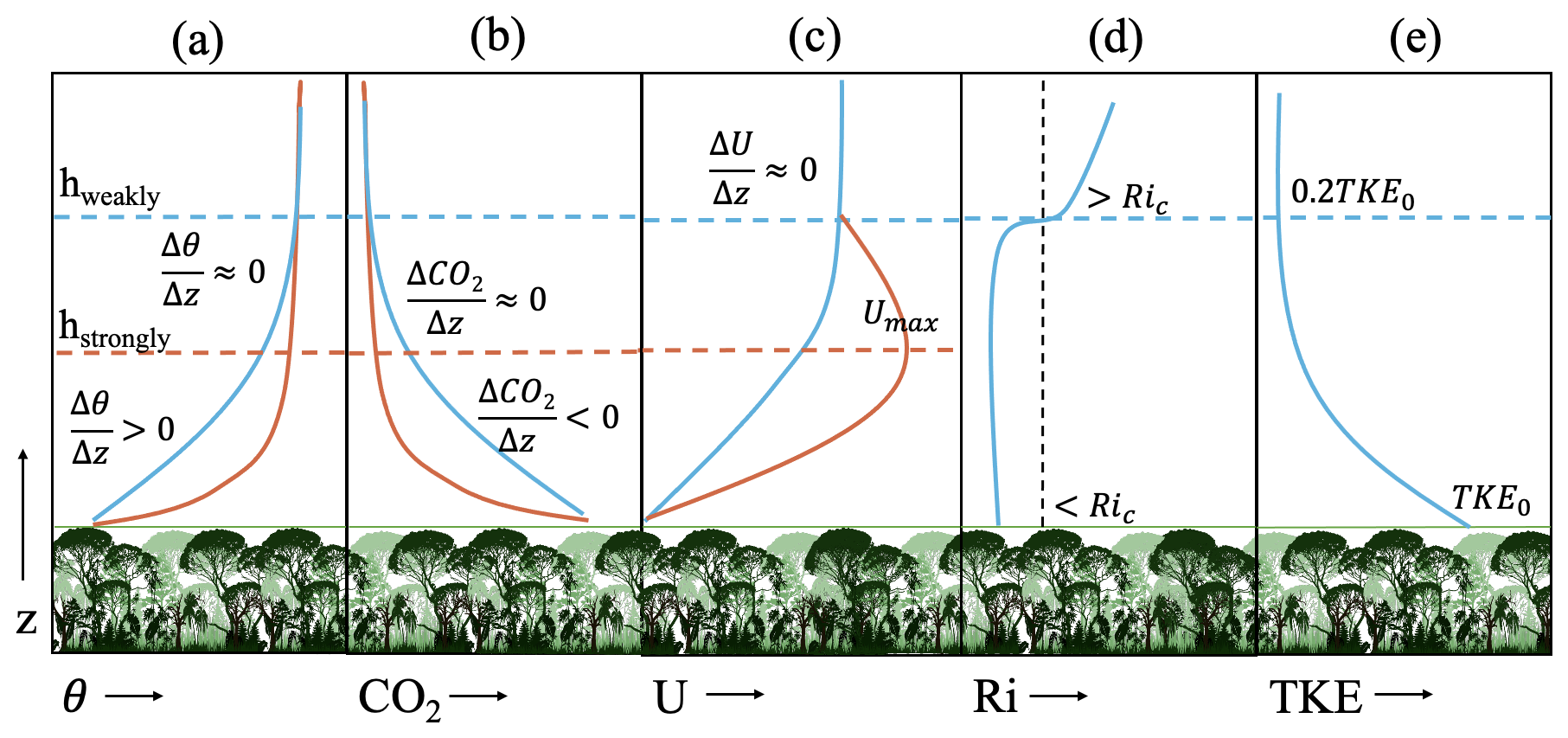
Figure 1 Five criteria for estimating the nocturnal boundary layer height (h_NBL): (a) potential temperature (θ), (b) CO₂, (c) horizontal wind speed (U), (d) Richardson number (Ri), and (e) turbulent kinetic energy (TKE). The blue lines represent the weakly stable regime and the red lines the strongly stable regime. The blue and red horizontal dashed lines indicate the estimated h_NBL of the weakly and strongly stable profiles, respectively. The vertical dashed black line in (d) represents the critical Richardson number (0.25).

In the NBL, θ increases with height above the canopy due to the cooling of the canopy top. However, this increase is not uniform, near the canopy, the vertical gradient is large, while toward the top of the NBL, the gradient weakens and gradually approaches zero. Therefore, we defined the NBL height as the lowest height at which the vertical gradient of θ falls below a prescribed low threshold (Fig. 1a). The threshold was defined as $\mathrm{3}\times {\mathrm{10}}^{-\mathrm{3}}$ m⁻¹. To determine the height at which this threshold was reached, θ was normalised as ${\mathit{\theta }}_{\mathrm{N}}=\mathit{\theta }/\mathrm{\Delta }\mathit{\theta }$, where Δθ is the difference between θ at 300 m (the top of the tower) and 32 m (the canopy top). This normalisation removes differences in temperature magnitude between nights and between the beginning and end of a given night. However, it does not alter the vertical temperature gradient used to estimate h_NBL. It is important to emphasise that θ_N is used only to estimate h_NBL, all other analyses are based on the observed θ.

For CO₂, the NBL is characterised by a negative CO₂ gradient with height, approaching 0 ppm m⁻¹ near the top of the stable layer. Utilising a similar method as for θ, we normalised the CO₂ gradient with height and chose a threshold. The threshold was defined as $\mathrm{2.5}\times {\mathrm{10}}^{-\mathrm{3}}$ m⁻¹ (Fig. 1b).

The U criterion was subdivided into two parts, based on whether a nocturnal low-level jet (NLLJ) (Blackadar, 1957) was observed above the NBL or not. In the measuring period of the CloudRoots-Amazon22 campaign, a weak NLLJ was observed during two nights (12–13 August and 17–18 August). When an NLLJ is present above the NBL, we defined h_U as the height where U=U_max (red line in Fig. 1c), because the NLLJ wind maximum forms on top of the stable NBL, where atmospheric friction approaches zero. This method was already found to yield trustworthy results above the Amazon canopy by Mendonça et al. (2026). When no NLLJ is present, we used the U gradient with height (Fig. 1c). Similar to θ and CO₂, we normalised the U gradient and chose a threshold of $\mathrm{2.5}\times {\mathrm{10}}^{-\mathrm{3}}$ m⁻¹.

The final two methods, based on Ri (calculated as the gradient Richardson number) and TKE, are only applied in the weakly stable regime, as sufficient turbulence above the canopy is required for the application of the criteria. We considered there is sufficient turbulence when Ri is below the critical Richardson number (Ri_c = 0.25) and TKE is greater than 0.10 m² s⁻² at the canopy top. Both methods are based on the assumption that all turbulence has dissipated in the residual layer, where the atmosphere is neutral. Therefore, h_Ri is found when Ri≥Ri_c (Fig. 1d) and h_TKE is determined at the first height where TKE= 0.2TKE₀, where TKE₀ is the observed TKE value at the canopy top. We chose to use a threshold of 20 % of the TKE values relative to the canopy top (instead of 5 %), due to predominantly stable conditions during the observation period (Fig. 1e).

The strongly stable periods were excluded for the following reasons. For Ri, because if Ri>Ri_c at the canopy top, the h_Ri will always be found at the canopy top, this might not be valid. For TKE, we need the distinction because if TKE<0.10 m² s⁻² at the canopy top, TKE₀ already approaches zero and does not show an 80 % decrease at higher elevations in the vertical profile.

2.3 Temporal evolution of stability within and above the canopy

To understand the importance of canopy-atmosphere interactions, we studied the temporal evolution of atmospheric stability, focusing on both the in-canopy atmosphere, the stable layer aloft and the interaction at the canopy-atmosphere interface. To compare the stability of the in-canopy and stable layer aloft, we introduce a bulk representation of Ri for both layers based on the work of Oliveira et al. (2013). For the stable layer above canopy, the Richardson number (Ri_atm) is defined by Eq. (1), and for the in-canopy layer including the canopy roughness layer, the Richardson number (Ri_can) is determined by Eq. (2). In the equations, the subscripts of θ and U, indicate the measurement heights of θ and U, g is the gravitational acceleration (9.81 m s⁻²), Δz is the difference in height between the two heights indicated in the subscripts and θ_ref is a reference temperature, taken as the potential temperature at the highest measuring level on ATTO tall tower (298 m).

$$\begin{array}{}\text{(1)}& {\displaystyle }& {\displaystyle }{\mathit{Ri}}_{\text{atm}}={\displaystyle \frac{g\mathrm{\Delta }z}{{\mathit{\theta }}_{\text{ref}}}}{\displaystyle \frac{{\mathit{\theta }}_{\mathrm{81}}-{\mathit{\theta }}_{\mathrm{35}}}{(U_{\mathrm{81}}-U_{\mathrm{35}}{)}^{\mathrm{2}}}}\text{(2)}& {\displaystyle }& {\displaystyle }{\mathit{Ri}}_{\text{can}}={\displaystyle \frac{g\mathrm{\Delta }z}{{\mathit{\theta }}_{\text{ref}}}}{\displaystyle \frac{{\mathit{\theta }}_{\mathrm{35}}-{\mathit{\theta }}_{\mathrm{5}}}{(U_{\mathrm{35}}-U_{\mathrm{5}}{)}^{\mathrm{2}}}}\end{array}$$

2.4 Quantifying canopy-atmopshere exchange of CO₂ and heat

To assess and quantify the coupling and exchange between the in-canopy atmosphere and the stable layer aloft, we evaluated the governing equations of TKE, heat and CO₂ for the selected strongly and weakly stable periods (Sect. 2.4.1).

To calculate the budgets using only our observations, we had to make the following two assumptions: (1) The atmosphere is horizontally homogeneous ($\frac{\stackrel{\mathrm{‾}}{\partial \mathit{\psi }}}{\partial x}=\frac{\stackrel{\mathrm{‾}}{\partial \mathit{\psi }}}{\partial y}=\mathrm{0}$) and (2) subsidence (vertically advective term) is negligible ($\stackrel{\mathrm{‾}}{w}=\mathrm{0}$). In addition, we aligned the coordinate system with the mean wind such that only the u component of the wind remained. We evaluated the governing equations using 30 min averaged data (indicated by the overbars). Vertical derivatives were calculated using one level above and below the desired height, except for the vertical divergence of the CO₂ flux, for which, due to a lack of measurements at all levels, a first-order method was employed, which may affect the accuracy of the calculations. The residual (R), or non-closure of the budgets, represents the uncertainty due to neglected terms of the governing equation that could not be calculated with our observations, and the observational uncertainty. In the following, we explain the strict selection of strongly and weakly stable regimes and each governing equation individually.

2.4.1 Criteria for assessing strongly and weakly stable regimes

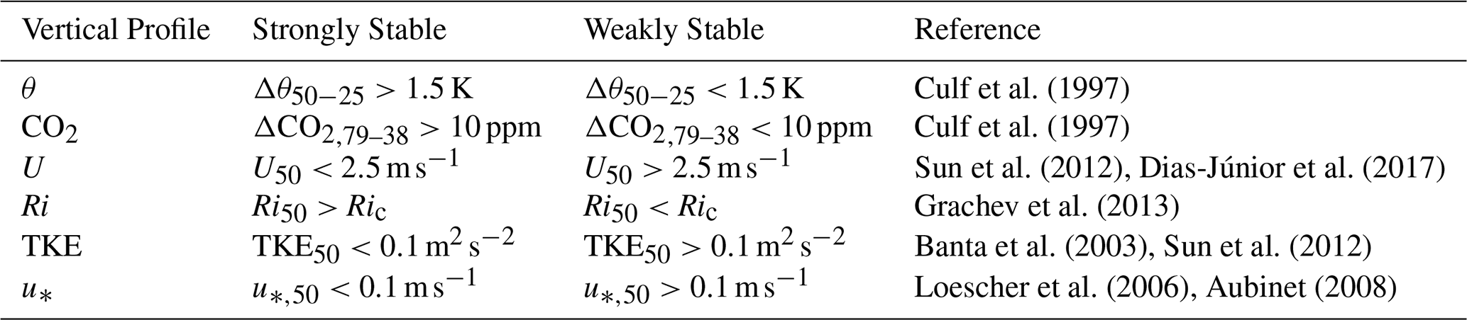
To distinguish between the strongly and weakly stable regimes, we employed six criteria based on: θ, CO₂, U, Ri, TKE, and friction velocity (u_*) from previous characterisation studies, adjusted to the CloudRoots-Amazon22 observations (Table 2). For θ and CO₂, we determined thresholds based on the degree of stratification. More specifically, the criteria for θ and CO₂ are based on gradients between 50–25 m for θ, and 79–38 m for CO₂. The reported thresholds are consistent with the strongly and weakly stable characterisation reported by Culf et al. (1999). The remaining four criteria are based on thresholds from the studies listed in Table 2 and were applied to observations at a height of 50 m.

Culf et al. (1997)Culf et al. (1997)Sun et al. (2012)Dias-Júnior et al. (2017)Grachev et al. (2013)Banta et al. (2003)Sun et al. (2012)Loescher et al. (2006)Aubinet (2008)

Table 2 Six criteria used to distinguish between strongly and weakly stable regimes for the CloudRoots-Amazon22 campaign. The subscripts indicate the measuring height(s) at which the criteria were validated. The Ri_c is taken as 0.25.

These prototypical NBL profiles are important for the parameterisation of the NBL in numerical weather and climate models (Edwards et al., 2020). Consequently, it is crucial to determine how well these prototypical representations align with nocturnal observations from the Amazon rainforest. Coarse canopy representations in numerical weather and climate models do not account for complex multilayer canopy structures (Bonan et al., 2021). Therefore, we base our selection on the atmospheric layer above the canopy to ensure a valid comparison with these prototypical model profiles.

2.4.2 Governing equation of TKE

Using the available observations, we analysed the TKE budget equation. Due to observational limitations, we simplified the TKE governing equation to five terms (Eq. 3). The net tendency of TKE ($\frac{\partial \stackrel{\mathrm{‾}}{e}}{\partial t}$), controlled by four terms, from left to right: the buoyant consumption (term 1), shear production (term 2), dissipation of TKE (term 3) and the residual term (R_TKE) (term 4). The R_TKE term contains processes that could not be quantified with current observations: the pressure fluctuation gradient term, the turbulent transport term and the horizontal and vertical advection of TKE. In Eq. (3), $\stackrel{\mathrm{‾}}{{\mathit{\theta }}_v}$ represents the virtual potential temperature in K, $\stackrel{\mathrm{‾}}{w^{\prime }{\mathit{\theta }}_{\mathrm{v}}^{\prime }}$ the kinematic heat flux in K m s⁻¹ and $\stackrel{\mathrm{‾}}{u^{\prime }{w}^{\prime }}$ the momentum flux in m² s⁻². The dissipation (ϵ) is calculated with a Fast Fourier Transform (FFT) from the u-wind component. The calculation of ϵ is done utilising the method from Hartogensis and de Bruin (2005). FFT spectra were checked for the presence of an inertial range. The average dissipation rate was calculated only if the slope deviated by less than 20 % from the theoretical $\mathrm{5}/\mathrm{3}$ slope and the root mean square error of ϵ was less than 30 % of its block-average value, otherwise, the ϵ value was rejected.

$$\begin{array}{}\text{(3)}& {\displaystyle }{\displaystyle \frac{\partial \stackrel{\mathrm{‾}}{e}}{\partial t}}={\displaystyle \frac{g}{\stackrel{\mathrm{‾}}{{\mathit{\theta }}_{\mathrm{v}}}}}\stackrel{\mathrm{‾}}{w^{\prime }{\mathit{\theta }}_{\mathrm{v}}^{\prime }}-\stackrel{\mathrm{‾}}{u^{\prime }{w}^{\prime }}{\displaystyle \frac{\partial \stackrel{\mathrm{‾}}{u}}{\partial z}}-\mathit{ϵ}+R_{\text{TKE}}\end{array}$$

2.4.3 Governing equation of heat

Using the available observations we analysed the governing equation of heat (Eq. 4). In Eq. (4) the net tendency of θ ($\partial \stackrel{\mathrm{‾}}{\mathit{\theta }}/\partial t$), is controlled by three terms, from left to right: the turbulent transport of heat (term 1), the vertical longwave radiative divergence (atmospheric longwave cooling rate from here onward) (term 2), and R_θ (term 3). Here, $\stackrel{\mathrm{‾}}{w^{\prime }{\mathit{\theta }}^{\prime }}$ is the heat flux in K m s⁻¹, $\stackrel{\mathrm{‾}}{\mathit{\rho }}$ is the air density in kg m⁻³, c_p the specific heat of air at constant pressure (1004 $\mathrm{J}{\mathrm{K}}^{-\mathrm{1}}{\mathrm{kg}}^{-\mathrm{1}}$) and $\stackrel{\mathrm{‾}}{Q}$ the net longwave radiation in W m⁻², which is defined positive towards the surface. The R_θ encompasses the molecular diffusion term, the latent heating term and the horizontal and vertical advection of heat (Stull, 1988). We do neglect the molecular diffusion because of its small magnitude compared to the other terms in the atmosphere and the latent heat flux, because a previous study by González-Armas et al. (2025) estimated latent heat fluxes that approach 0 W m⁻² above the canopy during the night.

Longwave radiation observations during CloudRoots-Amazon22 were scarce, only one sensor (at 75 m) measured incoming and outgoing longwave radiation. As a result, the atmospheric longwave radiative cooling rate ($\frac{\mathrm{1}}{\stackrel{\mathrm{‾}}{\mathit{\rho }}{c}_p}\frac{\partial \stackrel{\mathrm{‾}}{Q}}{\partial z}$) could not be determined from our observations. We therefore estimated the atmospheric longwave cooling rate using the Radiative Transfer for Energetics + RRTM for General Circulation Model – Parallel (RTE + RRTMGP) (Pincus et al., 2019). Specifically, we used the open-source C++ interface of RTE + RRTMGP (van Heerwaarden et al., 2026). To run the model, we used temperature and moisture vertical profiles from the ECMWF Reanalysis 5th Generation data (ERA5) (Hersbach et al., 2020). The ERA5 profiles were downscaled with the “Large-eddy simulation and Single-column model–Large-Scale Dynamics” or (LS)²D in short (van Stratum et al., 2023). Finally, we ran the model utilising default clear sky settings and disabled shortwave radiation. To test the reliability of the model output, we compared tower observations with ERA5 data (Appendix A). The temperature and moisture profiles agree with each other, with a maximum difference of 2 K in the temperature profiles and 0.004 ppmv for the volume mixing ratio (vmr). We consider these differences sufficiently small to provide a realistic estimate of the atmospheric longwave cooling rate with the RTE + RRTMGP model. This assumption was confirmed when we compared the model output at 75 m to the tower observations (Appendix A), which show an absolute mean difference of 6.92 W m⁻² and an associated standard error of 3.90 W m⁻².

$$\begin{array}{}\text{(4)}& {\displaystyle }{\displaystyle \frac{\partial \stackrel{\mathrm{‾}}{\mathit{\theta }}}{\partial t}}=-{\displaystyle \frac{\partial \stackrel{\mathrm{‾}}{w^{\prime }{\mathit{\theta }}^{\prime }}}{\partial z}}+{\displaystyle \frac{\mathrm{1}}{\stackrel{\mathrm{‾}}{\mathit{\rho }}{c}_p}}{\displaystyle \frac{\partial \stackrel{\mathrm{‾}}{Q}}{\partial z}}+R_{\mathit{\theta }}\end{array}$$

2.4.4 Governing equation of CO₂

Finally, we analysed the governing equation of CO₂ (Eq. 5), using our observations. In the equation, the net CO₂ tendency ($\partial \stackrel{\mathrm{‾}}{{\mathrm{CO}}_{\mathrm{2}}}/\partial t$), controlled by from left to right: the turbulent transport of CO₂ (term 1) and the residual term $R_{{\mathrm{CO}}_{\mathrm{2}}}$ (term 2). Here $\stackrel{\mathrm{‾}}{w^{\prime }{{\mathrm{CO}}_{\mathrm{2}}}^{\prime }}$ is the CO₂ flux in ppm m s⁻¹. Similar to R_θ, $R_{{\mathrm{CO}}_{\mathrm{2}}}$ encompasses the molecular diffusion term, horizontal and vertical advection of CO₂ and potential atmospheric sources of CO₂. We neglected the molecular diffusion because of its small magnitude compared to the turbulent transport, and assumed there is no production or destruction of CO₂ in the atmosphere above the canopy.

$$\begin{array}{}\text{(5)}& {\displaystyle }{\displaystyle \frac{\partial \stackrel{\mathrm{‾}}{{\mathrm{CO}}_{\mathrm{2}}}}{\partial t}}=-{\displaystyle \frac{\partial \stackrel{\mathrm{‾}}{w^{\prime }{{\mathrm{CO}}_{\mathrm{2}}}^{\prime }}}{\partial z}}+R_{{\mathrm{CO}}_{\mathrm{2}}}\end{array}$$

3 Results

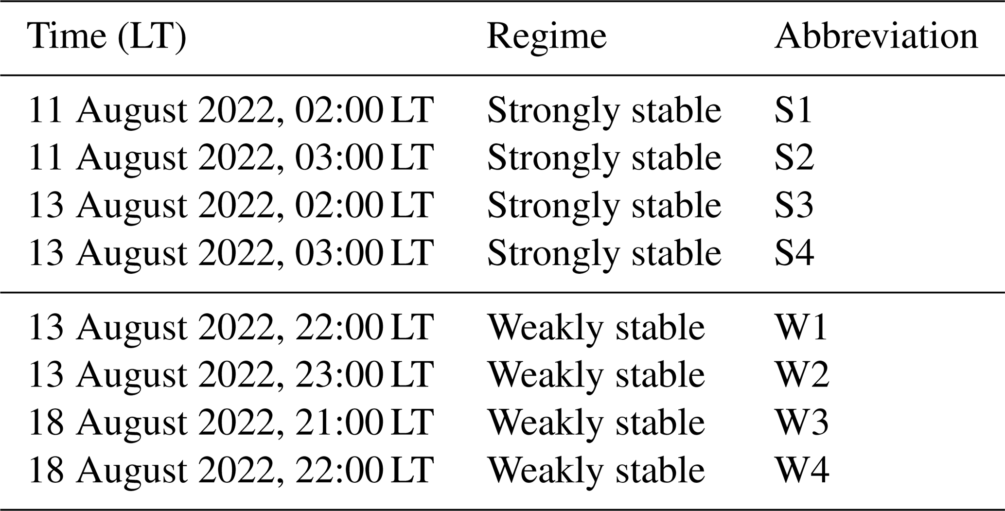
The results are presented in three sections. Section 3.1 describes the evolution of the h_NBL over time and compares the five estimation methods (Sect. 2.2). Section 3.2 describes the temporal evolution, thereby distinguishing between the within- and above-canopy layers. Both Sect. 3.1 and 3.2 make use of the complete data range of the CloudRoots-Amazon22 period (8–19 August). Finally, in Sect. 3.3, we evaluate the governing equations utilising the nights classified as strongly and weakly stable, based on the six strict criteria (Table 2). We found only eight hours during which all six strongly or weakly stable criteria were valid (Table 3), representing 6 % of the observations. These hours were distributed across four nights, with each night contributing two consecutive hours (Table 3). The non-selected data were characterised by sudden intermittent bursts, layers of elevated turbulence or other non-stationary nocturnal effects. The fact that only a small fraction of the observations adhered to either regime underscores the significant nocturnal variability on both an intra-night and inter-night basis.

Table 3 Selected times for the weakly and strongly stable regimes, with the abbreviations used further in the study. Times are indicated in LT (UTC−4).

3.1 Nocturnal boundary layer height

We found values of h_NBL ranging from 74 to 298 m across all criteria (Fig. 2), with h_Ri yielding the lowest estimate and h_U the highest. The average of five criteria is between 142–164 m throughout the night (Fig. 2a – grey line). The large observed variation within our study period can be linked to alternating strongly and weakly stable periods. With the selected hours in Table 3, we can find that in our strictly defined strongly stable regimes we estimated h_NBL to be 133 m (five-method mean S1, S2, S3, and S4) while it was 165 m (five-method mean W1, W2, W3 and W4) in the weakly stable regime.

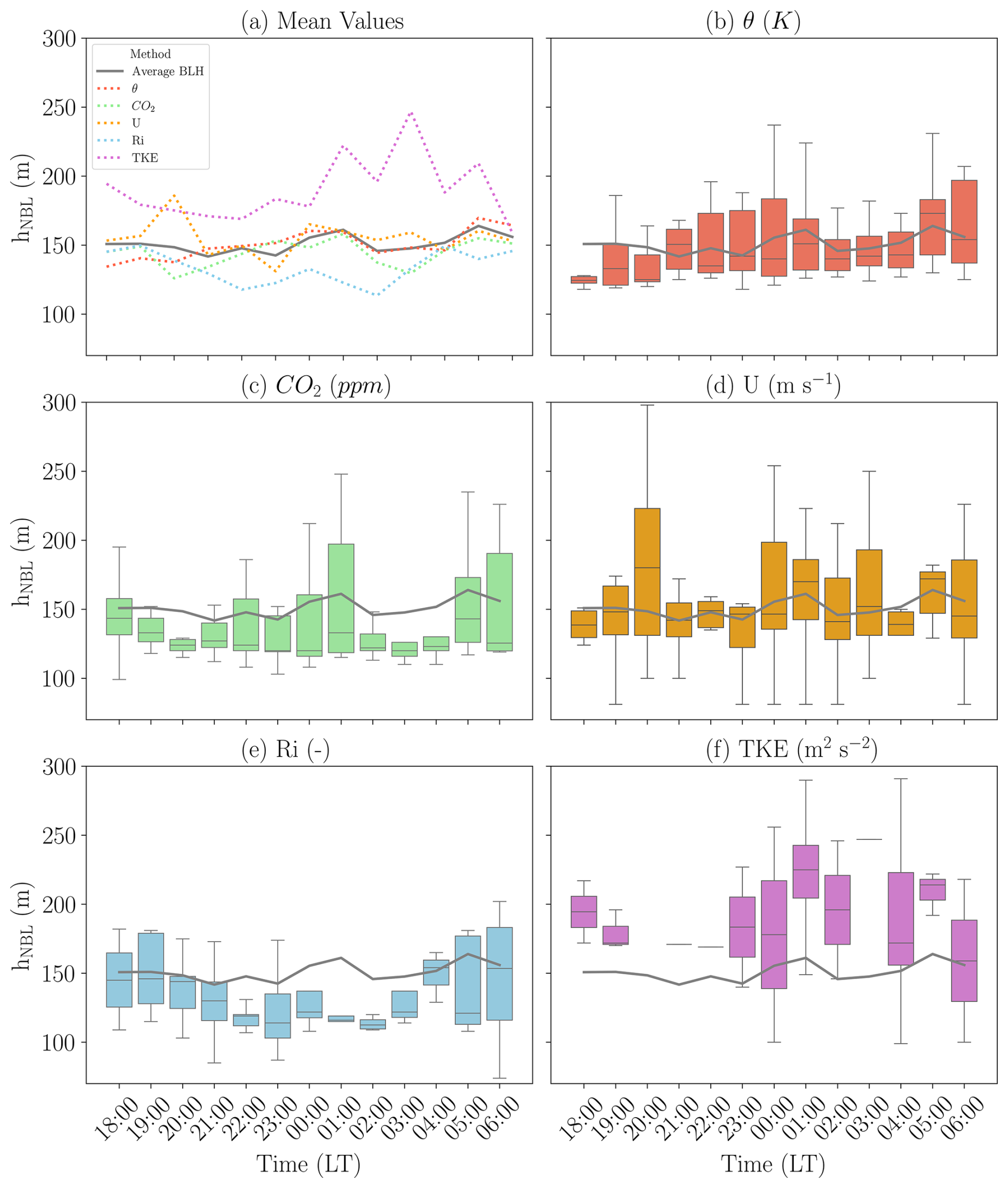
Figure 2 Hourly nocturnal boundary layer height in LT (UTC-4), estimated for the period between 8–19 August 2022. Panel (a) gives the mean boundary layer height for each of the five criteria (θ, CO₂, U, Ri and TKE) and the average of those five criteria (grey line). The remaining five graphs give the variation between the nights for every hour, for (b) potential temperature (θ), (c) CO₂, (d) wind speed (U), (e) Richardson number (Ri), and (f) turbulent kinetic energy (TKE). Here, the grey line represents the five-criterion mean boundary layer height.

The estimation of h_θ (Fig. 2b) closely follows the mean, with an average value of 150±27.1 m. The variation in h_θ can be attributed to the variability in the strength of the thermal stratification both intra- and inter-nightly. The stratification strength decreases when turbulent mixing occurs, which increases h_θ; conversely, h_θ remained low in the absence of turbulent mixing.

The $h_{{\mathrm{CO}}_{\mathrm{2}}}$ is estimated to be 145±42.2 m (Fig. 2c) which is slight below the average. Interestingly, the median of $h_{{\mathrm{CO}}_{\mathrm{2}}}$ remained around 140 m throughout the night, indicating that the observed variation was driven by a few exceptionally high $h_{{\mathrm{CO}}_{\mathrm{2}}}$ values. We hypothesise that these higher values were caused by bursts of intermittent turbulence, which transported CO₂ from within the canopy aloft (Karipot et al., 2006; Oliveira et al., 2013). This influx of CO₂ disrupted the strong vertical gradient, resulting in higher calculated values of $h_{{\mathrm{CO}}_{\mathrm{2}}}$.

Estimates of h_U (Fig. 2d) are found to be 156±46.5 m. The large variation in h_U is attributed to variable wind conditions during the campaign (Appendix B). The variation was strongly influenced by nights with almost linear vertical wind profiles (high h_U) and nights with an NLLJ (low h_U). Linear wind profiles were observed on the nights between 13–17 August. In these nights, the observed h_U were all ≥167 m. Weak NLLJ, with maximum wind speeds of 5.5 m s⁻¹, were observed during the nights of 12–13 August and 17–18 August. On the nights when the NLLJ was observed, the low-level wind (between 35–100 m) was from a North-northeastern direction. This same wind direction at ATTO has been found to originate from an area with low surface roughness by Mendonça et al. (2025), promoting stable stratification. Additionally, Northeastern winds have been associated with low elevated jet noses by Souza et al. (2026). Both findings are consistent with our observations; during these nights, we observed low-level jet nose heights between 80–100 m, low wind speeds at the top of the tower (≤3.0 m s⁻¹), and shallow NBLs (≤135 m).

For h_Ri and h_TKE, it is important to stress that these values were only calculated during periods with sufficient turbulence (weakly stable periods). Additionally, the estimations are potentially influenced by the presence of elevated layers of enhanced turbulence, which may disrupt the methods. The limited number of calculations particularly influenced results for h_TKE, as it could only be calculated in 20 % of the analysed hours. The estimation of h_Ri had an average of 134±29.5 m (Fig. 2e). We observed that h_Ri is often significantly lower than h_θ and $h_{{\mathrm{CO}}_{\mathrm{2}}}$, during turbulent periods, raising questions as to whether this method accurately reflects the underlying dynamics. The h_TKE is calculated to be 193±50.9 m (Fig. 5f), which is higher than average. The significant variation may be partly attributed to the limited number of estimations. Additionally, we observe that the TKE often did not reduce by 80 % within the vertical profile. It is possible that the frequent occurrence of very stable conditions complicated the application of this method during the CloudRoots-Amazon22 period, as previous studies at the ATTO site have yielded reliable results using similar turbulence-based methods (Mendonça et al., 2025; Souza et al., 2026).

The h_NBL above the Amazon rainforest has been investigated in a limited number of studies. All these studies reported h_NBL values ranging from 80 to 250 m (Oliveira et al., 2018; Carneiro and Fisch, 2020; Mendonça et al., 2025, 2026; Souza et al., 2026). We compare our results a bit more carefully to the three studies that also used ATTO data. Two estimated h_NBL utilising the vertical turbulence observations installed at ATTO (Mendonça et al., 2025; Souza et al., 2026) and one using the NLLJ nose height (Mendonça et al., 2026). The studies report h_NBL values ranging from 81 to 247 m, with Souza et al. (2026) specifically finding 120±28 m for the 2022 dry season. While this range is consistent with our results, slight differences persist. Such variations were anticipated, given that the different criteria are governed by distinct physical processes.

Overall, we consider the range, derived from all criteria together, to yield a stable representation of h_NBL during variable turbulent regimes. With this finding, we also show that gradient methods give reliable estimations of h_NBL. These gradient methods can be useful in NBL studies, particularly for locations where no vertical turbulence profiles are available.

3.2 Temporal evolution of stability within and above the canopy

The temporal evolution of the vertical atmospheric structure differs within and above the canopy (Fig. 3). At the canopy – atmosphere interface, between 25 (24) and 81 (79) m, we observe an increase (decrease) in the θ (CO₂) gradient from 0.040 K m⁻¹ (−0.09 ppm m⁻¹) to 0.046 K m⁻¹ (−0.51 ppm m⁻¹) throughout the night. In contrast, below the canopy (between 5–25 m), the θ (CO₂) gradient decreased (increased) from 0.067 K m⁻¹ (−1.77 ppm m⁻¹) to 0.015 K m⁻¹ (−0.69 ppm m⁻¹).

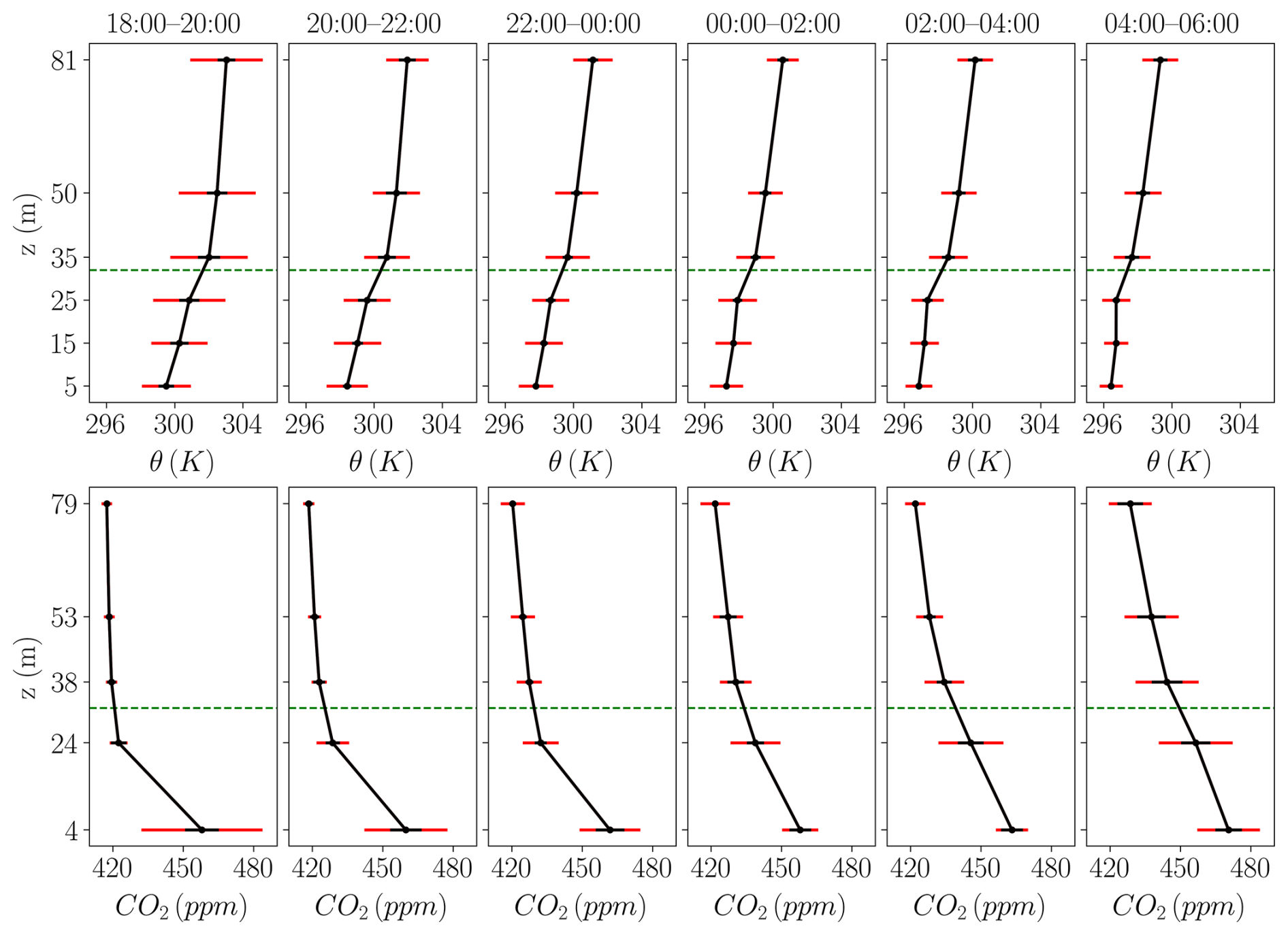
Figure 3 Mean profiles for the CloudRoots-Amazon22 nights between 8–19 August of potential temperature (θ) (top) and CO₂ (bottom), averaged for every 2 h. Red error bars are the standard deviation between the different nights, and the black error bars indicate the average 2 h bin variation. The striped green horizontal line indicates the aerodynamic canopy top at 32 m.

Above the canopy, the atmospheric stratification strengthens during the night, while the within-canopy layer mixes over time. After sunset (18:00–20:00 LT), below the canopy, a shallow stable daytime layer was present within the canopy. The shallow stable layer has been observed to form during daytime by González-Armas et al. (2025). Throughout the night, the atmospheric stratification within the canopy layer weakens, enabling air mixing and thereby leading to better mixed CO₂ profiles throughout the canopy layer.

We hypothesise that the mixing within the canopy layer originates from the cold layer forming in the dense canopy crown, roughly between 15–30 m (Gomes Alves et al., 2023). In this layer, the vegetation biomass cools down, creating a locally cold layer, which promotes sinking motions and enhances turbulence in the canopy layer. Enhanced turbulence within the canopy has also been reported in previous studies (Kruijt et al., 2000; Santos et al., 2016). Santos et al. (2016) found that a radiative imbalance of $\le -$40 W m⁻² is needed to make this sinking motion possible, this threshold was met during most nights during CloudRoots-Amazon22 campaign (not shown). In addition, we can confirm the downward motion of cold air by turbulence observations. When we inspect the selected hours used in Sect. 3.3 (Table 3) as an example, we observed a positive heat flux ($\stackrel{\mathrm{‾}}{w^{\prime }{\mathit{\theta }}^{\prime }}$) during S2, S3, S4, and W3 within the canopy layer, which can be associated to the downward movement of cold air ($w^{\prime }<\mathrm{0}$ and ${\mathit{\theta }}^{\prime }<\mathrm{0}$) (Appendix C).

In addition to the observed temporal evolution, we must acknowledge the large variability between the nights. The largest variation is observed just after sunset (18:00–20:00 LT) and before sunrise (04:00–06:00 LT). After sunset, the large potential temperature variation, driven partially by temperature changes within two-hour windows (black error bars), can be attributed in part to strong longwave radiative cooling of the canopy at the onset of the night (Stull, 1988). In contrast, the large variation in the CO₂ molar fraction at 4 m is mainly driven by inter-night variability (red error bars). This pronounced nocturnal CO₂ variability may result from three mechanisms: (1) the strength of the stable stratification, which is influenced by radiative cooling and the extent of CO₂ transport from the stable canopy layer into the atmosphere aloft (Moonen et al., 2025), (2) the absolute temperature and moisture conditions, influencing the respiration rate (Lloyd and Taylor, 1994; Zanchi et al., 2012) and amount of CO₂ stored in the stable daytime layer and (3) the preference of CO₂ to build up in low topographical points (de Araújo et al., 2010), where low-level horizontal advection can cause large differences in CO₂ molar fraction at the surface. Because of the non-homogeneous influence of the mechanisms over time, it remains hard to tell the dominant mechanism, this might well be variable between nights.

Just before sunrise, we observe large variation in CO₂ molar fractions throughout the vertical profile. The large variation can be explained by enhanced mixing during sunrise. In a previous study by Dupont et al. (2024), they found that the transport of CO₂ in the early morning differs between low and high wind speeds. The variable wind conditions during the CloudRoots-Amazon22 period (Appendix B), may explain the large contrast between nights.

3.2.1 Coupling between the canopy-atmosphere interface

Stability evolves in opposing directions above and within the canopy, characterised by stabilising trends aloft and mixing within the canopy (Fig. 4). This divergence between the two layers is most pronounced during the predominantly strongly stable night (10–11 August, red line, Fig. 4) and least pronounced during the predominantly weakly stable night (18–19 August, blue line, Fig. 4).

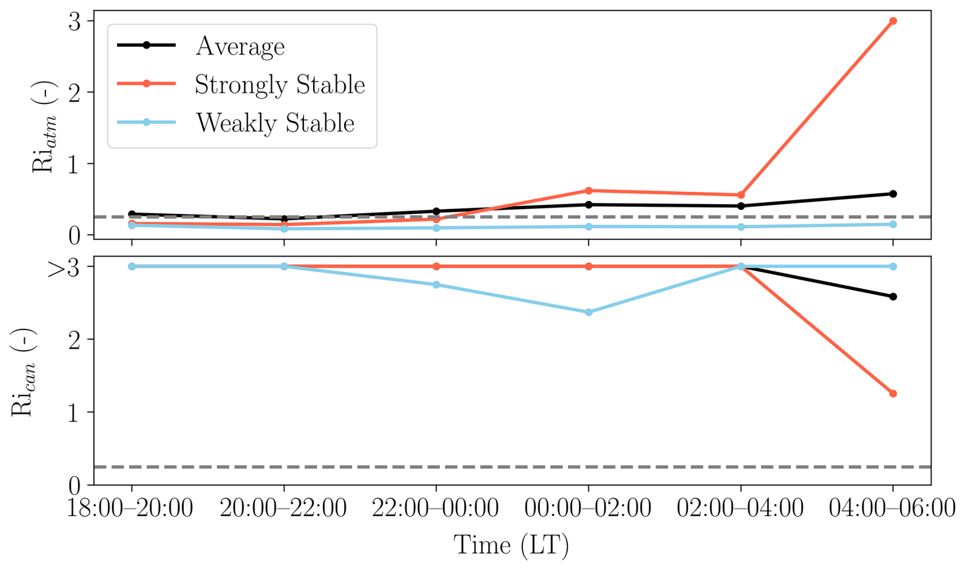
Figure 4 Two-hour average temporal evolution of the Richardson number above canopy (top) and Richardson number below canopy (bottom). Where the black line is the average of the nights between 8–19 August, the red line represents the strongly stable night of 10–11 August 2022 and the blue line the weakly stable night on the night of 18–19 August 2022. The striped grey line indicates the critical Richardson number (0.25).

Above the canopy, Ri_atm increases across all three cases during the night. However, it increases most significantly in the strongly stable night (red line). In the weakly stable night (blue line), Ri_atm remained below Ri_c throughout the night, indicating continuous turbulence. Contrary to Ri_atm, Ri_can decreased over time for the average and strongly stable night (only visible between 04:00–06:00 LT). Note that it never reaches Ri_c due to the persisting stable gradient between 25–35 m (Fig. 3), which we included in the Ri_can calculation to prevent it from becoming unstable due to low wind speeds below 25 m. In the weakly stable night, Ri_can decreased between 22:00–02:00 LT, indicating a coupling between the stable and canopy layer, where mixing between the two layers is possible. The observation of mixing in the weakly stable regime was also reported by Santos et al. (2016). Interestingly, the Ri_can for the weakly stable night does not show a similar decrease at the end of the night, indicating less well-mixed conditions within the canopy at sunset. The lack of mixing at the end of the night might be due to a weaker stable temperature gradient over height caused by mixing throughout the night, preventing the sinking motion of cold air.

Based on the findings above, we discuss the degree of coupling of the canopy and atmospheric layers during the two regimes. Following the decoupling parameter proposed by de Kauwe et al. (2017), we estimated a similar factor based on Ri_atm and Ri_can. We identified the layers as decoupled when Ri_atm>Ri_c and Ri_can<Ri_c, and coupled when Ri_atm<Ri_c, leading to Ri_can>Ri_c by the end of the night. Applying this parameter to the profiles in Fig. 5e confirms that the strongly stable profile is decoupled, whereas the weakly stable profile remains coupled, permitting interaction between the two layers. This distinction between regimes controls the accumulation of CO₂ below the canopy and, consequently, the magnitude of the flux during sudden increases in turbulence (Acevedo et al., 2016).

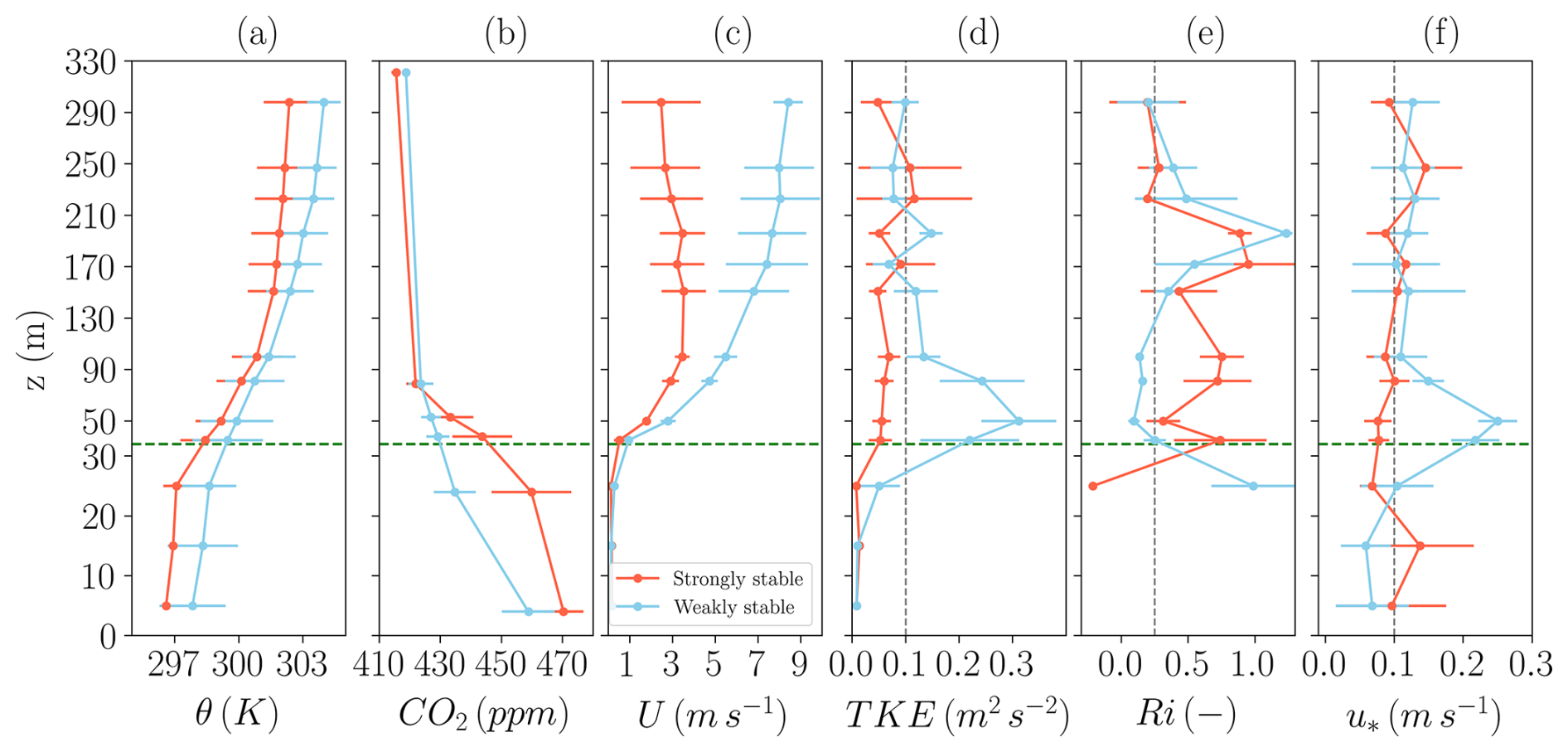
Figure 5 Vertical profiles above and below the canopy, the dashed green line indicates the aerodynamic top of the canopy (32 m). Profiles are shown for (a) potential temperature (θ), (b) CO₂, (c) wind speed (U), (d) turbulent kinetic energy (TKE), (e) Richardson number (Ri) and (f) friction velocity (u_*). In the figure, the red line shows the average of the strongly stable cases (S1, S2, S3, and S4), with the standard deviation in error bars. The blue lines show the same, but for the weakly stable cases (W1, W2, W3, and W4). The vertical lines in (d), (e), and (f) represent the threshold values (at 50 m) used to select the strongly and weakly stable profiles, being 0.1 m² s⁻², 0.25 and 0.1 m s⁻¹ respectively.

3.3 Exchange of CO₂ and heat at the canopy-atmosphere interface

We evaluated the governing equations of TKE (Sect. 3.3.1), heat (Sect. 3.3.2) and CO₂ (Sect. 3.3.3) above the canopy, for the periods classified as strongly and weakly stable (Table 3). Vertical profiles for all six criteria differ distinctly between the two regimes (Fig. 5). The strongly stable vertical θ profile shows a larger temperature gradient between 25–50 m (2.08 K) than the weakly stable profile (1.29 K) (Fig. 5a). For CO₂ (Fig. 5b), a similar pattern is observed: the CO₂ gradient between 38–79 m is larger for the strongly stable regime (−21.8 ppm) than during the weakly stable regime (−5.5 ppm). These differences are attributed to a combination of the nocturnal temporal evolution of θ and CO₂, as well as the influence of variable turbulent activity during the regimes.

Horizontal wind speed clearly differs between the strongly and weakly stable regimes (Fig. 5c). Already at 25 m, the wind speed and gradient with height in the weakly stable profile are enhanced compared to the strongly stable profile. At 50 m, the threshold of 2.5 m s⁻¹ is reached in the weakly stable profile, but not for the strongly stable profile. Additionally, in the weakly stable regime, TKE (Fig. 5d) and u_* (Fig. 5f) at 50 m exceed the thresholds (Table 2) and Ri<Ri_c (Fig. 5e), in contrast to the strongly stable regime. The observed differences vanish above 200 m for TKE, Ri, and u_*, suggesting that the turbulent regime does not significantly influence the residual layer. The observed differences between the regimes are consistent with a previous study by Dias-Júnior et al. (2017).

3.3.1 Observational interpretation of the TKE budget

We evaluated the terms of the TKE budget (Eq. 3) above the canopy one by one, distinguishing between the strongly and weakly stable regimes (Fig. 6). In Fig. 6, the average logarithmic fitted profiles (least-squares polynomial) are plotted for the four strongly stable (S1, S2, S3, and S4) and four weakly stable (W1, W2, W3, and W4) profiles indicated in Table 3. The shaded area indicates the standard deviation between these four selected hours for both the strongly and weakly stable regimes.

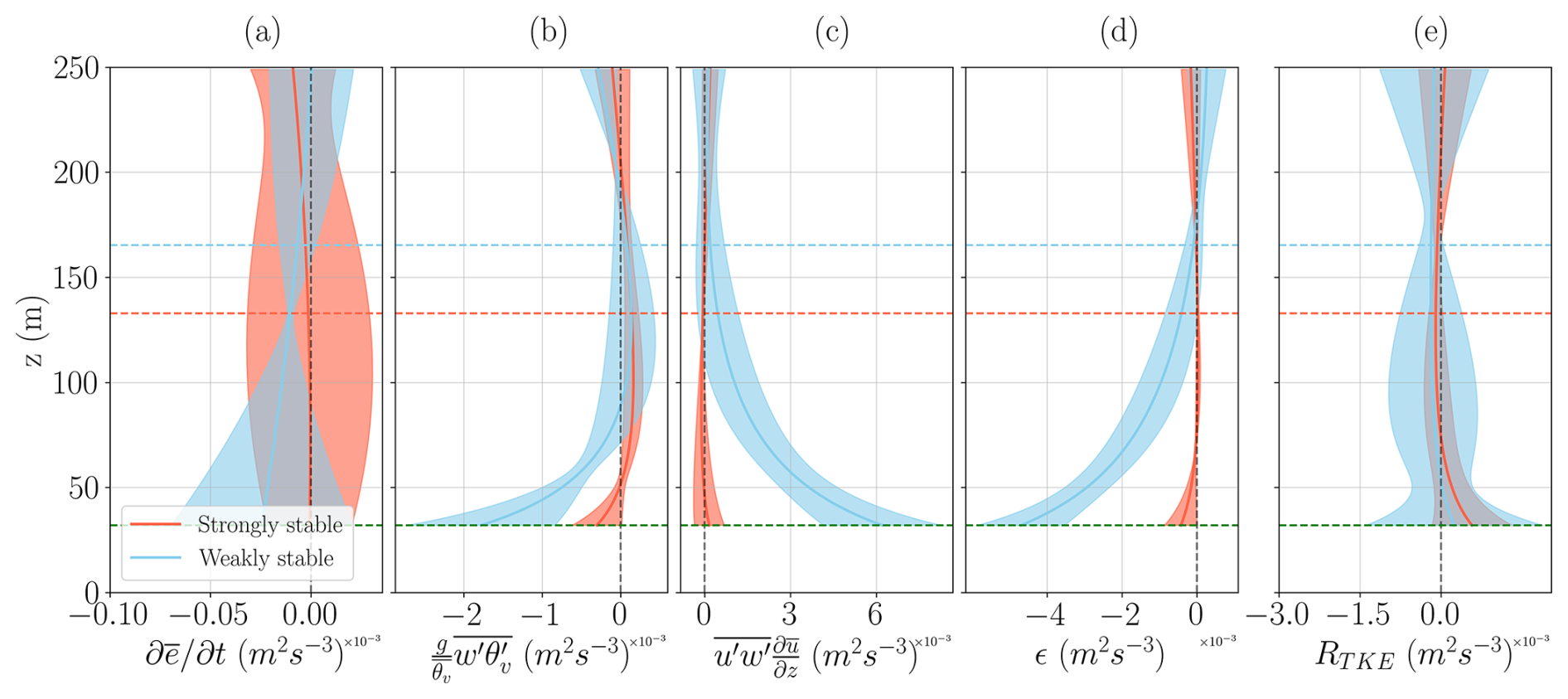
Figure 6 Conservation of turbulent kinetic energy (TKE), according to Eq. (3), based on the selected prototypes described in Table 3. Here, the red line represents the average of the four strongly stable profiles (S1, S2, S3, and S4), and the shaded area represents the standard deviation. Blue is the same, but for the four weakly stable profiles (W1, W2, W3, and W4). The graphs represent the terms of the TKE equation: (a) the TKE tendency, (b) the buoyant consumption, (c) the shear production, (d) dissipation, and (e) the residual. The horizontal lines indicate the average h_NBL, calculated for the strongly (red) and weakly (blue) stable regimes.

For both the strongly and weakly stable regimes, the TKE tendency (Fig. 6a) is 10–100× smaller compared to the individual terms and shows no significant difference between the regimes. The buoyancy term (Fig. 6b) is most negative at the canopy top and increases with height. For the weakly stable regime, buoyancy is more negative ($-\mathrm{1.70}\times {\mathrm{10}}^{-\mathrm{3}}\pm \mathrm{0.94}\times {\mathrm{10}}^{-\mathrm{3}}$ m² s⁻³) than for the strongly stable regime ($-\mathrm{0.30}\times {\mathrm{10}}^{-\mathrm{3}}\pm \mathrm{0.31}\times {\mathrm{10}}^{-\mathrm{3}}$ m² s⁻³), indicating, that there is almost no vertical turbulent movement in the strongly stable regime. The shear term at the canopy top (Fig. 6c), is significantly larger for the weakly stable regime ($\mathrm{6.20}\times {\mathrm{10}}^{-\mathrm{3}}\pm \mathrm{2.05}\times {\mathrm{10}}^{-\mathrm{3}}$ m² s⁻³) than for the strongly stable regime ($\mathrm{0.16}\times {\mathrm{10}}^{-\mathrm{3}}\pm \mathrm{0.52}\times {\mathrm{10}}^{-\mathrm{3}}$ m² s⁻³). This is in accordance with Mironov and Sullivan (2016), who found that the magnitude of shear is about three times larger than buoyancy in the weakly stable regime.

The dissipation rate is largest in magnitude at the canopy top and decreases logarithmically with height. In the weakly stable regime the dissipation is more negative ($-\mathrm{4.69}\times {\mathrm{10}}^{-\mathrm{3}}\pm \mathrm{0.25}\times {\mathrm{10}}^{-\mathrm{3}}$ m² s⁻³) than for the strongly stable regime ($-\mathrm{0.43}\times {\mathrm{10}}^{-\mathrm{3}}\pm \mathrm{0.44}\times {\mathrm{10}}^{-\mathrm{3}}$ m² s⁻³). Our results for dissipation are in also in line with Mironov and Sullivan (2016), which find dissipation to have a magnitude of shear minus buoyancy.

The residual (Fig. 6e), which approaches zero with height, represents measurement and calculation errors, vertical and horizontal advection of TKE and the effect of pressure fluctuations. Previous studies have indicated that vertical and horizontal advection and pressure fluctuations can be important for the TKE balance above dense canopies (Dwyer et al., 1997; Vickers and Thomas, 2013; Chen and Chamecki, 2023). However, our results suggest that these terms are small relative to the buoyancy, shear, and dissipation terms under weakly stable conditions. Under strongly stable conditions, they may make an important contribution to the residual, but it remains hard to quantify the magnitude of the terms included in the residual. Further research incorporating high-frequency observations and large-eddy simulations with multilayer canopy representations could provide deeper insight into the magnitude of these terms in the residual under both stability regimes.

3.3.2 Observation interpretation of the heat budget

Secondly, we evaluated the governing equation of heat, which quantifies the heating of the atmosphere as a function of the turbulent transport of heat (driven by shear), the atmospheric longwave cooling rate and other processes represented by the residual (Fig. 7). The temperature tendency is negative for both the strongly ($-\mathrm{0.29}\pm \mathrm{1.06}$ K h⁻¹ at the canopy top) and weakly ($-\mathrm{0.37}\pm \mathrm{0.49}$ K h⁻¹ at the canopy top) stable regime (Fig. 7a). However, especially in the strongly stable regime, the temperature tendency varies stongly, caused by the variation between S1, S2, S3, and S4. Above the canopy, at 50 m, the temperature decreased during S2 (−1.7 K h⁻¹) and S4 (−0.03 K h⁻¹) but increased during S1 (0.3 K h⁻¹) and S3 (0.3 K h⁻¹). Two processes can cause the increase in temperature: (1) non-turbulent sub-mesoscale effects in strongly stable periods (Oliveira et al., 2018), and (2) the presence of the NLLJ during S3 and S4 which mixes air from above downward, increasing the temperature (Smedman, 1988; Mahrt, 1998; Karipot et al., 2006).

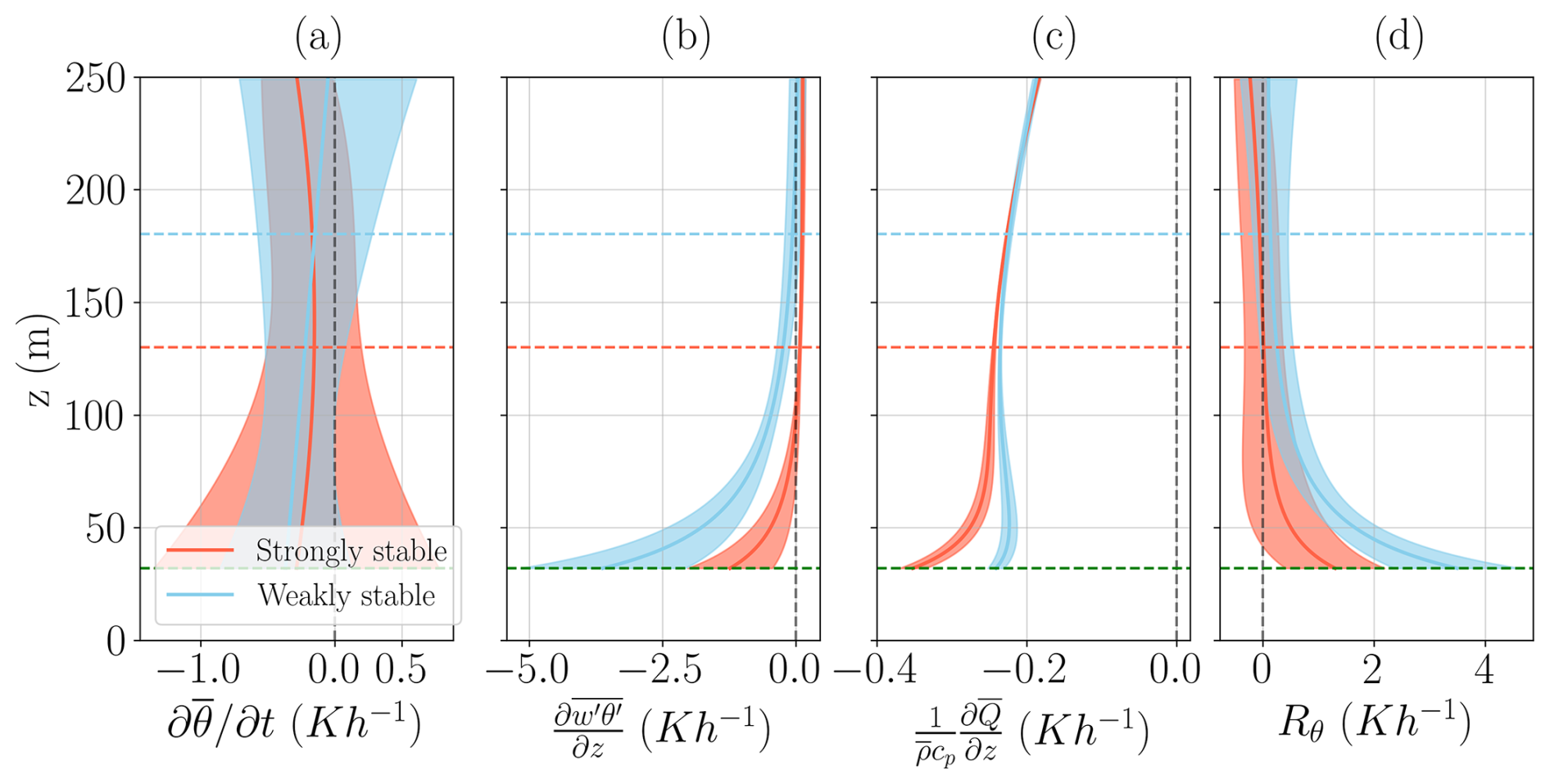
Figure 7 Conservation of heat, according to the simplified form of Eq. (4), based on the selected prototypes described in Table 3. Here, the red line represents the average of the four strongly stable profiles (S1, S2, S3, and S4), and the shaded area is the standard deviation. Blue is the same, but for the four weakly stable profiles (W1, W2, W3, and W4). The graphs represent the terms of the heat equation: (a) the temperature tendency, (b) the turbulent transport of heat, (c) radiative heating, and (d) the residual. The horizontal lines indicate the average h_NBL, calculated for the strongly and weakly stable regimes.

The second term, turbulent transport of heat, decreases logarithmically with height, and approaches zero above h_NBL (Fig. 7b). The weakly stable profile showed a more negative turbulent heat-flux divergence at the canopy top ($-\mathrm{3.62}\pm \mathrm{1.54}$ K h⁻¹), than the strongly stable profile ($-\mathrm{1.23}\pm \mathrm{0.79}$ K h⁻¹). This difference is consistent with the enhanced mechanical production of turbulent kinetic energy observed in the weakly stable regime (Fig. 6c), which promotes turbulent mixing between the cold canopy layer and the warmer atmosphere aloft. Compared to a grassland surface, turbulent transport of heat above the Amazon canopy is up to 2 K h⁻¹ higher (Stull, 1988). The difference between the two surface types can be explained by the higher surface roughness of the forest canopy, which enhances turbulent mixing.

The atmospheric longwave cooling rate decreases logarithmically with height above the canopy top (Fig. 7c). The strongly stable regime ($-\mathrm{0.35}\pm \mathrm{0.02}$ K h⁻¹ at the canopy top) shows a higher atmospheric longwave cooling rate than the weakly stable regime ($-\mathrm{0.24}\pm \mathrm{0.35}$ K h⁻¹ at the canopy top). Cloud cover likely reduced the longwave cooling rate during W1 and W2 (Appendix D), partly explaining the difference between the two regimes. However, the differences between the two regimes are small compared to the −2 K h⁻¹ cooling rate over a grass surface reported by Stull (1988). The lower cooling at the canopy top is explained by the non-homogeneous canopy surface, where the most intense cooling occurred not above the canopy top, but within the canopy, where the leaf density is highest.

Similar to the TKE equation, a large residual remained in the heat equation. At 50 m the residual is 0.74±0.62 K h⁻¹ for the strongly stable case and 1.75±0.40 K h⁻¹ for the weakly stable case. Temperature advection may explain a significant part of the residual. A horizontal temperature gradient of 0.15 K km⁻¹ downwind would already lead to a heat advection of about 1.0 K h⁻¹ in the strongly stable regime and 1.6 K h⁻¹ in the weakly stable regime at 50 m height. Multiple processes can initiate horizontal temperature differences in the Amazon rainforest; examples are differences in land use or soil moisture content (Al-Kayssi et al., 1990; Gash and Nobre, 1997). To the East of the ATTO, a swampy area is located, which likely increased nocturnal temperatures, this may explain the positive residual given the observed dominant South-eastern wind direction (Appendix B). Additionally, the residual term includes effects of temperature dissipation and measurement and calculation uncertainties. These uncertainties include the estimation of the atmospheric longwave cooling rate. This term was calculated using ERA5 data rather than direct observations, which introduces additional uncertainty into our estimation.

3.3.3 Observational interpretation of the CO₂ budget

Finally, we evaluated the governing equation of CO₂. The terms of the governing equation of CO₂ are depicted per term in Fig. 8 and are described one by one in this section. For the CO₂ tendency (Fig. 8a), we observe that the CO₂ tendency is positive (1.62±1.96 ppm h⁻¹ at the canopy top) for the weakly stable regime (CO₂ increasing over time) and negative ($-\mathrm{5.61}\pm \mathrm{8.23}$ ppm h⁻¹ at the canopy top) for the strongly stable regime. The positive CO₂ tendency in the weakly stable regime can be caused by mixing of CO₂-enhanced air from within the canopy upward. In the strongly stable regime, two processes can cause the negative CO₂ tendency: (1) the NLLJ mixing of CO₂-depleted air downwards (Smedman, 1988; Mahrt, 1998; Karipot et al., 2006) and (2) drainage of CO₂ at the surface (Goulden et al., 2006; de Araújo et al., 2010). The drained air at the surface is replaced by subsiding CO₂-depleted air from above, decreasing the CO₂ concentration. However, significant variation is observed in CO₂ tendency in the strongly stable regime. This variation is driven by S3, where an intermittent event before the period caused a CO₂ increase (7.1 ppm h⁻¹) that strongly impacts our results due to the low temporal resolution of the data.

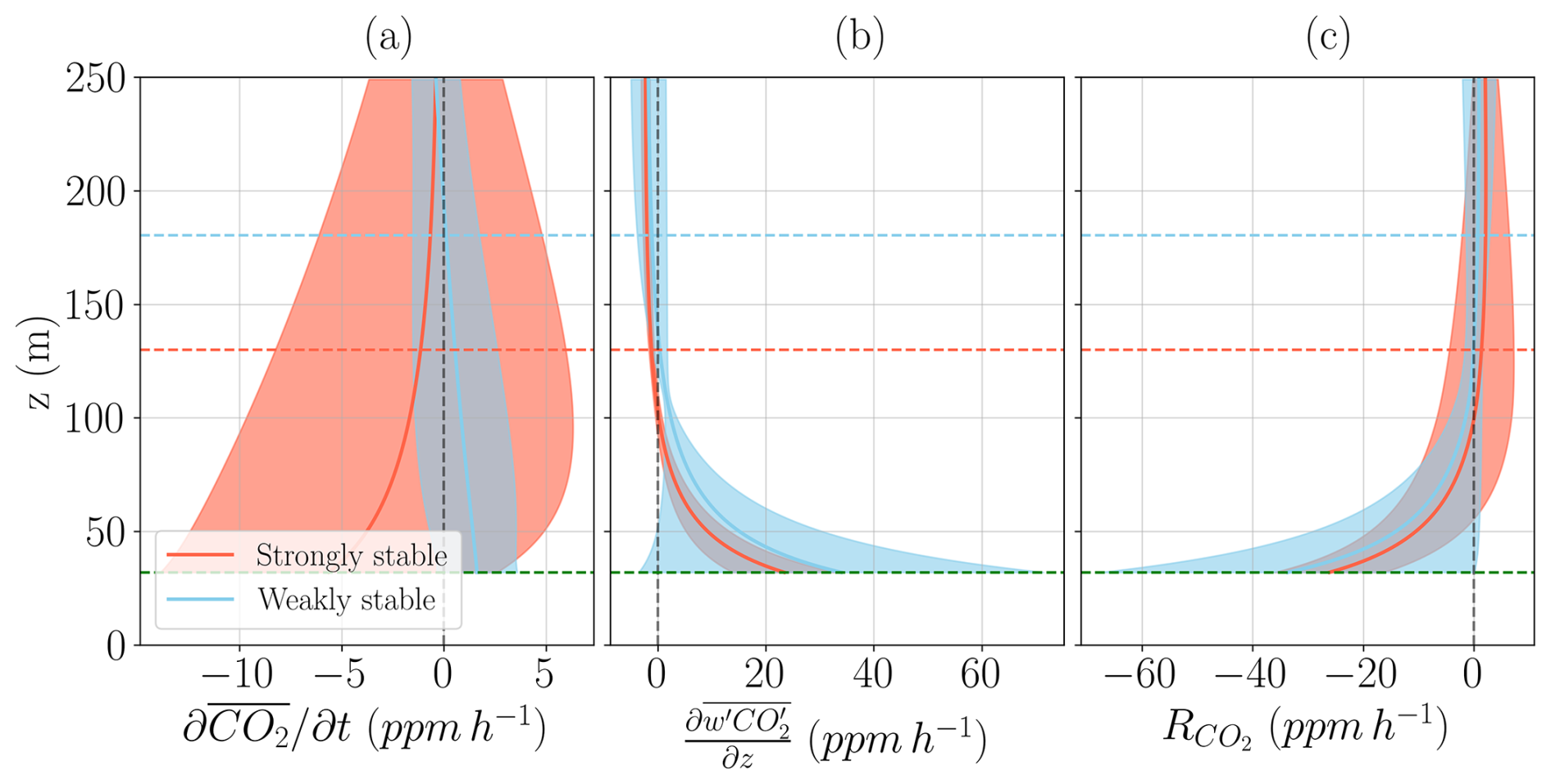
Figure 8 Conservation of CO₂, according to the simplified form of Eq. (5), based on the selected prototypes described in Table 3. Here, the red line represents the average of the four strongly stable profiles (S1, S2, S3, and S4), and the shaded area is the standard deviation. Blue is the same, but for the four weakly stable profiles (W1, W2, W3, and W4). The graphs represent the terms of the CO₂ equation: (a) the CO₂ tendency, (b) the turbulent transport of CO₂, and (c) the residual. The horizontal lines indicate the average h_NBL, calculated for the strongly and weakly stable regimes.

For the turbulent transport of CO₂, we observed a higher turbulent transport of CO₂ during the weakly stable regime (33.94±37.45 ppm h⁻¹ at the canopy top) than in the strongly stable regime (23.39±9.54 ppm h⁻¹ at the canopy top). The high standard deviation of turbulent CO₂ transport within the weakly stable regime is attributable to the disparity between the observed periods. Specifically, W3 and W4 exhibited low transport (± 3 ppm h⁻¹ at 50 m) resulting from minimal flux divergence between 50–81 m, implying that turbulence penetrated higher into the atmosphere, as the magnitude of the fluxes was similar to W1 and W2. This stands in contrast to W1 and W2, where substantial turbulent transport (± 15 ppm h⁻¹ at 50 m) was observed. Additionally, in both the weakly and strongly stable regimes, can the temporal and spatial variability in soil CO₂ efflux, driven by changes in, for example, soil temperature and moisture content (Zanchi et al., 2012), influence the magnitude of the observed turbulent exchange above the canopy.

Following findings that daytime shear and canopy ejections significantly contribute to carbon fluxes (Moonen et al., 2025), we assessed the significance of nocturnal fluxes. During weakly stable periods, the average flux at 50 m was 3.82 $\mathrm{\mu }\mathrm{mol}{\mathrm{m}}^{-\mathrm{2}}{\mathrm{s}}^{-\mathrm{1}}$ (maximum 6.38 $\mathrm{\mu }\mathrm{mol}{\mathrm{m}}^{-\mathrm{2}}{\mathrm{s}}^{-\mathrm{1}}$ in W2). In line with previous studies (Culf et al., 1997; Mahrt, 2011; Oliveira et al., 2013, 2018) our results confirm that nocturnal CO₂ fluxes can be significant. Conversely, the decoupled strongly stable regime showed a minimal average flux of 0.16 $\mathrm{\mu }\mathrm{mol}{\mathrm{m}}^{-\mathrm{2}}{\mathrm{s}}^{-\mathrm{1}}$.

Similar to the other two budget equations, a significant residual remains for the budget equation of CO₂. The negative residual (Fig. 8c) is largely explained by horizontal advection. Airplane measurements in the morning (09:00 LT) of 18 August (de Feiter et al., 2025a) showed a CO₂-depleted area East of ATTO, creating a horizontal gradient of −0.68 ppm km⁻¹ at 09:00 LT. With the gradient and the measured horizontal wind speed, we can estimate an advection magnitude of −6 ppm h⁻¹ at 50 m, accounting for a large part of the ±10 ppm h⁻¹ residual. This advection was likely stronger at the canopy top and during the night, because of the logarithmic nocturnal CO₂ profile (Fig. 5b) and the dilution of the CO₂ gradient by mixing in the morning transition that had already started at 09:00 LT (Dupont et al., 2024). Additionally, part of the residual can be attributed to calculation and measurement errors, and contributions from the neglected terms.

4 Discussion

The CloudRoots-Amazon22 measuring campaign enabled us to provide an in-depth description of the dry season NBL above the Amazon rainforest. However, there are multiple limitations to its applicability. First, the results are likely not directly applicable to the wet season due to the differing cloud and precipitation patterns (Biscaro et al., 2021) and turbulent activity (Mendonça et al., 2023), which change boundary layer structure and development. Second, our observations are limited to one year; therefore, multi-year climate variability cannot be accounted for, even though previous studies by Carneiro and Fisch (2020) and Souza et al. (2026) found that there is multi-year variability in NBL characteristics. Third, because of the large spatial topography and forest heterogeneity in the Amazon rainforest, our observations and results are not directly applicable to the whole Amazon basin. For example, in the lower valleys, soil and vegetation conditions change, influencing the temperature and trace gas dynamics (Pinheiro-Oliveira et al., 2026). Fourth, our analysis is limited by a two-week measurement period, from which only eight nocturnal profiles adhered to the prototypical NBL often used in model parameterisations. These eight hours represent only about 6 % of the nocturnal data, reflecting the substantial variability of the Amazonian nocturnal boundary layer and raising questions about whether idealised model parameterisations capture the observed diversity. Such discrepancies between observed vertical fluxes and prototypical regimes were also noted by Mahrt and Acevedo (2023), who emphasised that nocturnal boundary layer structure is not limited to the prototypical structures even over seemingly flat surfaces. Consistent with these findings, we show that similarly complex structures occur in the Amazonian NBL above the canopy. This complexity is further enhanced by interactions with the within-canopy atmosphere, introducing complexity at the lower boundary of the above canopy stable stratification. Collectively, these limitations both complicate the application of our findings to other seasons and regions within the Amazon rainforest and underscore the importance of measuring horizontal terms both within and above the canopy.

With the study limitations in mind, our discussion focuses on the following three points: (1) the uncertainties associated with nocturnal flux data, (2) the influence of clouds as a disturbing factor of the NBL prototypical framework, and (3) recommendations for future research.

4.1 Uncertainties associated with nocturnal flux data

Eddy covariance measurements in general, and thus also the data collected during the CloudRoots-Amazon22 campaign, are challenging to use during the night (Loescher et al., 2006; Aubinet, 2008). With eddy covariance devices, the turbulent transport of momentum, heat and CO₂ by eddies is measured. Within a strongly stable NBL, the limited vertical extent of small eddies, combined with low turbulence intensity and non-linear processes, introduces uncertainties in the data series. Additionally, 30 min averaging intervals may filter the inherent intermittency of turbulence (Oliveira et al., 2013, 2018; Hicks et al., 2015), although such intermittency likely drives the variability observed within those periods. Investigating the underlying mechanisms and frequency of these intermittent events would require an analysis of shorter time intervals (five minutes or less). Therefore, leveraging high-frequency ATTO observations to quantify the influence of intermittent activity on CO₂ and temperature variability is an essential next step.

These future analyses could lead to improved NBL parameterisation by incorporating the effects of intermittent bursts. Such intermittency arises from a diversity of processes, including surface-layer interactions as described by van de Wiel et al. (2002a), van de Wiel et al. (2002b), as well as elevated layers of turbulence associated with NLLJs, and other mesoscale motions (Mahrt, 1999; Sun et al., 2015). Additionally, to capture complex canopy-atmosphere interactions, the model parameterisation should account not only for intermittent, but also for the complex, stability-dependent coupling between the NBL and the within-canopy layer.

4.2 Influence of clouds on the prototypical framework

In this study, we did not explicitly study the effect of clouds on the NBL evolution. However, Monahan et al. (2015) observed that cloudy conditions are more typical of the weakly stable regime. During the CloudRoots-Amazon22 observations, high clouds were, among other nights, observed during the first half of the night between 13–14 August (Appendix D). The presence of these clouds may have limited the development of a strongly stratified layer during the early part of the night, potentially contributing to the weakly stable atmospheric conditions observed during periods W1 and W2.

Additionally, daytime studies have found effects of clouds on trace gas transport from the canopy up into the atmosphere (Moonen et al., 2025; de Feiter et al., 2025a). The importance of the daytime clouds suggests that, also during the night, clouds could have a significant role in CO₂ exchange. So far, the influence of nocturnal clouds on this transport remains poorly understood and has only been evaluated in a few studies. Machado et al. (2024) observed that during the night the CO₂ molar fraction in the atmosphere decreases after a rainfall event, which was correlated with increased humidity, decreased temperature and radiation. Mendonça et al. (2023) found that the passage of nocturnal deep convective clouds can generate substantial upward ejections of CO₂ from the within-canopy air. The magnitude of these ejections depends on the amount of CO₂ stored within the canopy, which, as we show, is closely related to the prevailing nocturnal stability regime.

4.3 Future recommendations

Our findings indicate the need to include an explicit representation of the tall canopy (Bonan et al., 2021; Vilà-Guerau de Arellano et al., 2023) and improve representations to include the transition between weakly and strongly stable NBL, allowing for rapid intermittent periods (Maroneze et al., 2019). In addition, high-resolution measurements are vital to observe sinking motions of cold air into the canopy. Therefore, measurements of the upward and downward longwave radiation and temperature with high vertical resolution (±1 m) in the cooling layer (20–30 m) are advised. These measurements would also make it possible to validate the RTE + RRTMGP model output with observations, providing more confidence in our atmospheric longwave cooling rate estimate and the radiation model in general.

Finally, these observational studies could enable us to bridge the gap between one-layer and multilayer canopy models (Bonan et al., 2021). The advancement to multi-layer canopy models is crucial due to increasing model resolution, but even so, to improve model parameterisations in large-scale models. The high-resolution vertical observations are of great importance for validating state-of-the-art, multi-layer canopy models using large-eddy simulation techniques (Patton et al., 2016; Ma and Liu, 2019; Pedruzo-Bagazgoitia et al., 2023). These models have already proven to yield important improvements in representing canopy-atmosphere interactions, atmospheric stability and topographical effects. Therefore, we think the multilayer canopy models are the next step in improving the complex nocturnal vegetation-atmosphere interactions.

5 Conclusions

This observation-driven study aimed to investigate whether the prototypical NBL often used in parameterisations of numerical weather and climate models adequately captures the observed variability in the nocturnal Amazonian boundary layer. To this end, we analysed observations collected both within and above the canopy during two weeks of the CloudRoots-Amazon22 campaign in the dry season. We investigated the dynamical and radiative characteristics of the Amazonian NBL, focusing on the vertical distributions of heat and CO₂ from within the canopy to the overlying atmosphere. We characterised atmospheric stability both above and within the canopy by estimating h_NBL and analysing stability parameters. Following this, we quantified exchange between these layers using observations to evaluate the main terms in the governing equations for TKE, heat and CO₂. To interpret the observations from the perspective of idealised NBL parameterisations, we organise the profiles into weakly and strongly stable regimes based on the interplay between longwave radiative cooling, which drives stratification, and mechanically generated turbulence, which promotes mixing.

Our results revealed a shallow stable layer above the canopy, with heights varying between 142–164 m during the campaign nights, depending on the method used to estimate h_NBL. This substantial variation in h_NBL was driven by the interplay between wind shear and the atmospheric longwave cooling rate throughout the night. This resulted in alternating periods dominated by shear (weakly stable), resulting in high h_NBL (165 m) and periods dominated by the atmospheric longwave cooling rate (strongly stable), associated with low h_NBL (133 m). Within the canopy, the atmosphere transformed from stable at the beginning of the night to well-mixed at the end of the night. Well-mixed profiles of θ and CO₂ were most pronounced during the strongly stable regime. In this regime, limited shear at the canopy top caused a strongly stratified layer, with a temperature gradient of 2.1 K between 25–50 m, driven by the longwave radiative cooling rate, which initiated the sinking motion of the cold air downward from the canopy top, mixing the within canopy within-canopy layer. Above the mixed canopy layer, the strongly stratified layer limited the exchange of heat ($-\mathrm{1.23}\pm \mathrm{0.79}$ K h⁻¹) and CO₂ (19.74±8.11 ppm h⁻¹) across the canopy-atmosphere interface. In contrast, during the weakly stable periods, increased wind shear at the canopy top enhanced exchange of heat ($-\mathrm{3.62}\pm \mathrm{1.54}$ K h⁻¹) and CO₂ (29.13±31.75 ppm h⁻¹). The increased heat and CO₂ exchange in the weakly stable regimes confirm the coupled state of the canopy layer and atmosphere aloft. The coupling makes significant CO₂ fluxes of 3.52 $\mathrm{\mu }\mathrm{mol}{\mathrm{m}}^{-\mathrm{2}}{\mathrm{s}}^{-\mathrm{1}}$ possible. In contrast, canopy-atmosphere interactions are inhibited in the decoupled strongly stable regime, leading to a CO₂ flux of only 0.16 $\mathrm{\mu }\mathrm{mol}{\mathrm{m}}^{-\mathrm{2}}{\mathrm{s}}^{-\mathrm{1}}$. These contrasting responses were governed by the stability of both the within- and above-canopy layers, as well as by the turbulent exchange between them.

The study highlights substantial nocturnal variability both between and within nights, including considerable variability within narrowly defined stability regimes. Only approximately 6 % of observed profiles conform to prototypical NBL regimes, underscoring the need to revisit current parameterisations for Amazonian canopy environments. This study shows that to improve these representations, it is crucial to account for both non-stationary intermittent effects and within-canopy stability variation.

Appendix A: ERA5 and RTE + RRTMGP compared to tower observations

Figure A1 depicts ERA5 observations compared to tower observations of one selected strongly stable hour (S1) and one selected weakly stable hour (W1). The remaining selected hours in Table 3 are comparable to the two comparisons shown. We find that for S1, the temperature profiles of ERA5 and the tower are very similar. However, below the canopy, the difference between the model and observations increases (max 2 K). The volume moisture ratio (vmr) of S1 has an error of approximately 0.001 ppmv, but follows the same trend as observations. For W1, the ERA5 and tower observations are less similar. The error in temperature above the canopy has a maximum of 1.8 K, while the error below the canopy is similar to S1. The vmr of W1 has an error of approximately 0.004 ppmv at the canopy top, but decreases towards h_NBL.

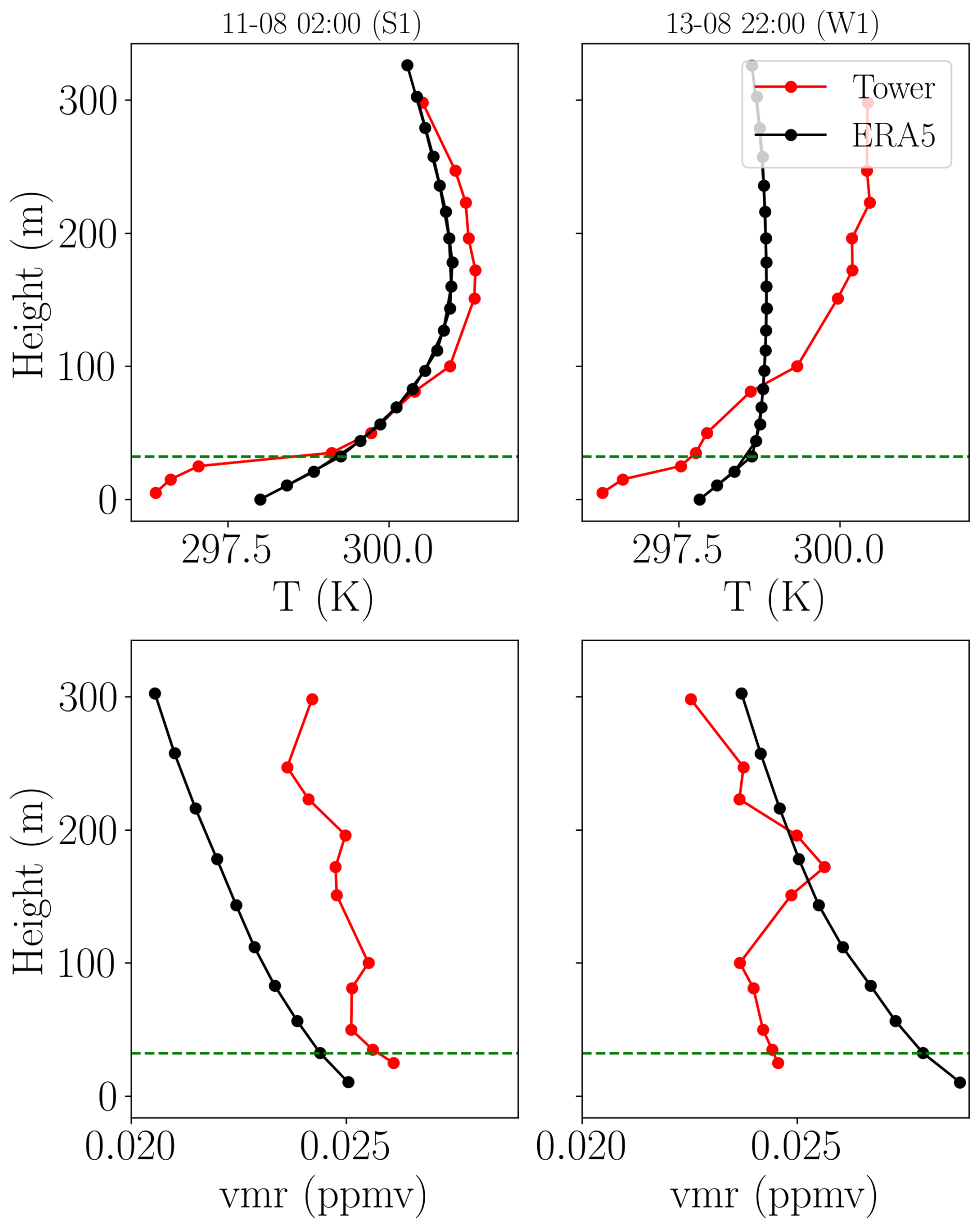
Figure A1 ERA5 vertical profiles (Black) of temperature (top) and volume moisture ratio (vmr) (bottom) compared to tower observations (red). The vertical profiles are from one strongly stable hour (S1) and one weakly stable hour (W1).

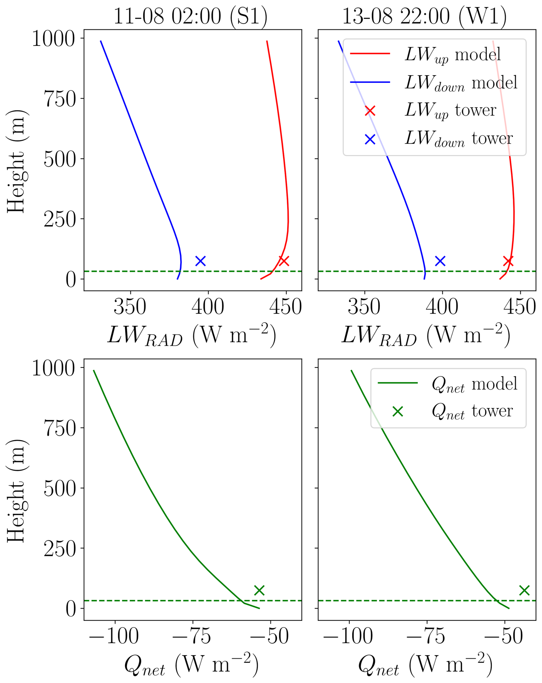
Figure A2 RTE + RRTMGP model output for S1 and W1. For the upgoing (red) and downward (blue) longwave radiation, and net longwave radiation (green). Together with the tower observations at 75 m (×).

Figure A2 depicts the RTE + RRTMGP model outcomes of upward and downward longwave radiation (top) and resulting net radiation (bottom), compared to the observations at 75 m. The difference between the model and observations is smallest for the upward longwave radiation (max 3.3 W m⁻²), and of similar magnitude for the downward (max 12.3 W m⁻²) and net radiation (max 11.5 W m⁻²).

Appendix B: Wind direction and speed

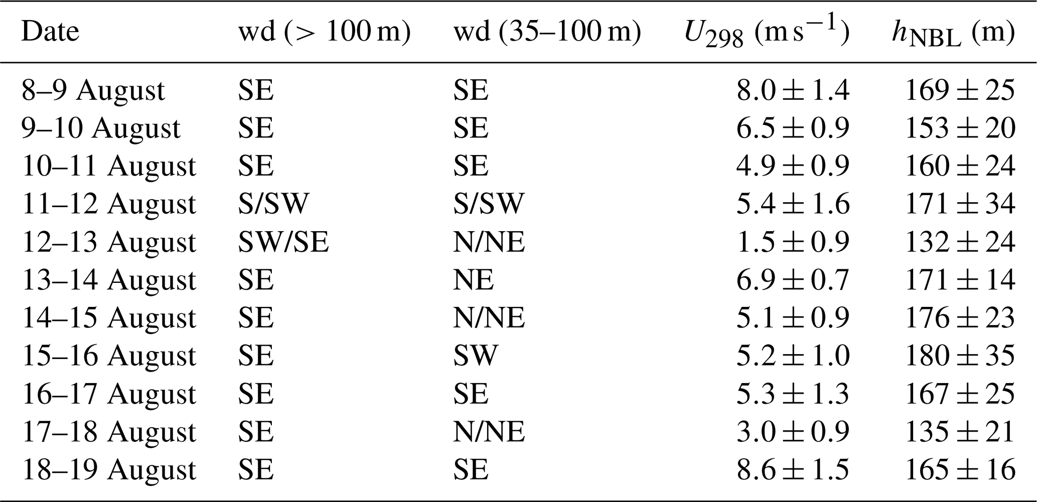
Table B1 Dominant observed wind directions (wd) above and below 100 m, wind speed range at the top of the tower (298 m), and mean h_NBL with standard deviations for the nights of the CloudRoots-Amazon22 campaign. Here the abbreviation for wd are defined as follows: South (S), Southeast (SE), Southwest (SW), North (N), Northeast (NE).

Appendix C: Measured eddy covariance fluxes of heat and CO₂ fluxes

The heat flux (Fig. C1) is plotted below for the selected periods for the strongly and weakly stable periods. We observe that in S2, S3, and S4, the heat flux increases below the canopy, indicating downward transport of cold air or upward transport of warm air. In the weakly stable atmosphere, the opposite happens; here, the heat flux becomes negative above the canopy, indicating upward motion of cold air or downward motion of warm air.

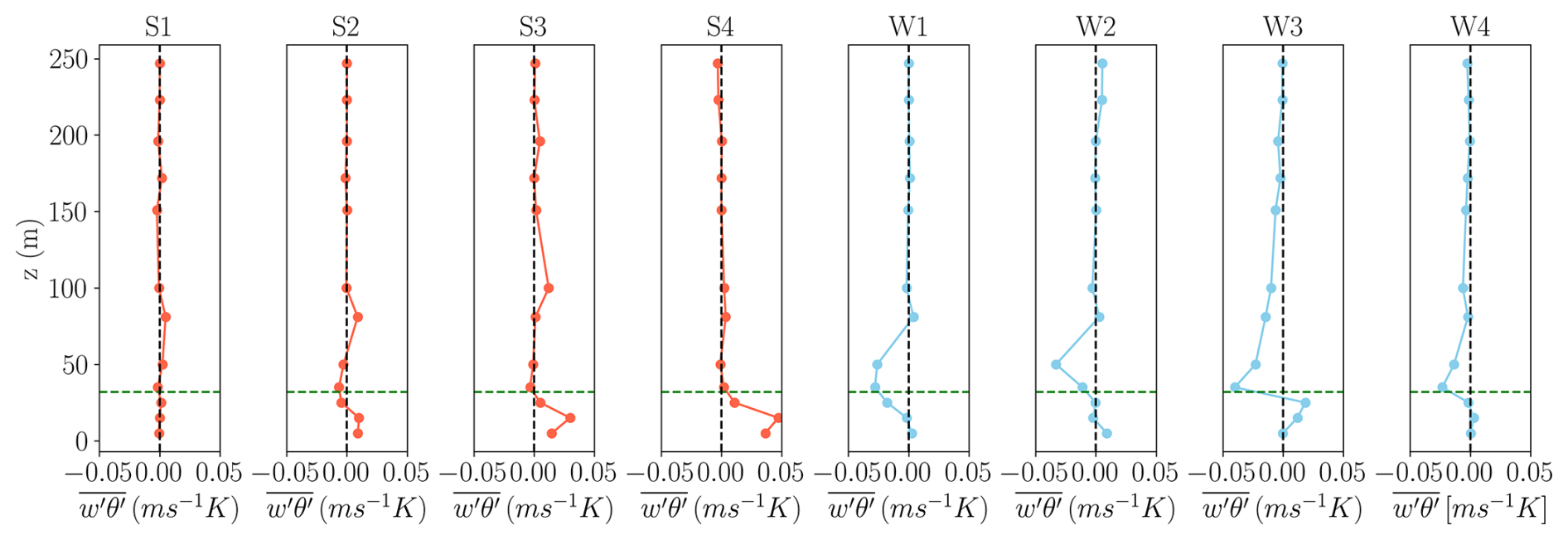
Figure C1 Eddy covariance heat fluxes above and below the canopy for the selected strongly and weakly stable periods. The canopy top (32 m) is depicted by the horizontal green dashed line.

Appendix D: Cloud observations and net longwave radiation

Cloud observations from the MIRA radar, during the nights from which the strongly and weakly stable profiles were selected, are plotted in Fig. D1. The blue Shallow cumulus (SCu) clouds around the top of the residual layer were found to be caused by high-moisture areas. On the night of 12–13 August (the night of S3 and S4), the MIRA radar observed some Cirrus (Ci) and Altostratus (As) clouds roughly 2 h after sunset and before sunrise. On the night of 13–14 August (night of W1 and W2), Ci and Cirrostratus (Cs) clouds were observed by the MIRA radar until midnight.

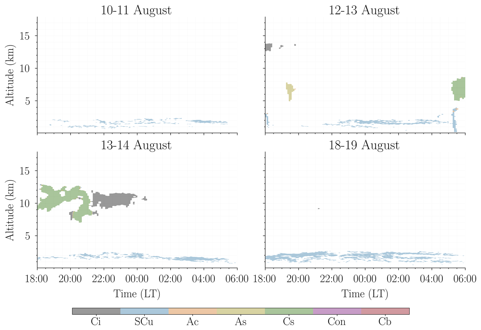
Figure D1 Clouds observed by the MIRA Doppler radar during the nights of 10–11 August, 12–13 August, 13–14 August, and 18–19 August. Where the nights start at sunset at 18:00 LT and end at sunrise at 06:00 LT. In the figure, the cloud abbreviations mean the following: cirrus (Ci), shallow cumulus (SCu), altocumulus (Ac), altostratus (As), cirrostratus (Cs), cumulus congestus (Con), and cumulonimbus (Cb).