Can radon help to improve methane emission estimates? Results from a dual-tracer inversion

A major source of uncertainty in inverse modelling of greenhouse gas emissions are deficits in atmospheric transport models, in particular in the description of vertical mixing within the planetary boundary layer (PBL). The properties of radon-222 (Rn) makes it a suitable natural tracer for vertical mixing in the PBL. When comparing the CH₄ model-data mismatch (MDM), i.e. the differences between the observed and modelled CH₄ concentrations, with the MDM of Rn, we found substantial correlations for several observation sites in central Europe in 2021 (the median CH₄-Rn MDM correlation coefficient is 0.6), indicating that a large part of the CH₄ and Rn MDM variability can be explained by common errors in the simulated (vertical) transport. We aim to exploit this information in a joint inversion for CH₄ and Rn by taking into account prior uncertainties and making use of the fact that the transport model error is correlated between the two gases. We use simultaneous CH₄ and Rn observations from 17 sites across central Europe in 2021. The dual-tracer CH₄-Rn inversion yields lower CH₄ fluxes in several countries covered by the observation sites compared to a single-tracer CH₄-only inversion without Rn information. The differences in country-total CH₄ fluxes between the dual-tracer and single-tracer inversions are on the order of a few percent and depend on the assumed uncertainty for the Rn prior fluxes. These findings underscore the importance of accurate Rn flux maps for fully leveraging the dual-tracer approach and enhancing the reliability of CH₄ flux estimates.

1 Introduction

Observations of the atmospheric mixing ratios of greenhouse gases (GHGs) provide independent information that is used within atmospheric transport inversions (Enting, 2002) to constrain (prior) estimates of GHG fluxes, e.g., from emission inventories and process-based land surface models (LSMs), by using an atmospheric transport model. In Bayesian inversion systems, the difference between observed and modelled atmospheric mixing ratios (the so-called model-data mismatch, MDM) is minimised by adjusting the prior fluxes and taking into account the uncertainties in the observations, the transport model, and the prior fluxes. Such top-down approaches have been used to estimate surface fluxes for all relevant GHGs, e.g., to study trends, interannual variability and seasonal cycles in fluxes at different spatial scales (e.g., Peylin et al., 2013; Bergamaschi et al., 2018; Chandra et al., 2022; Patra et al., 2022; Vojta et al., 2024), to verify emission inventories (e.g., Henne et al., 2016; Basu et al., 2020), or to benchmark process-based LSMs (e.g., Rödenbeck et al., 2018; Chang et al., 2023).

In recent years, methane (CH₄) has gained increasing attention due to its accelerating atmospheric growth rate over the past decade, the drivers of which are still not fully understood (Saunois et al., 2025). Moreover, CH₄ has about 30 times the global warming potential (over a 100-year time horizon) than carbon dioxide (CO₂) but a much shorter atmospheric lifetime of about 9 years, making the reduction of CH₄ emissions an effective option for limiting global warming in the near term (Saunois et al., 2025). At the Conference of the Parties (COP26) in autumn 2021, the “Global Methane Pledge” was launched with the aim of reducing global CH₄ emissions by at least 30 % by 2030 compared to 2020. Inverse modelling of CH₄ emissions is a powerful tool for monitoring progress towards meeting such targets, but is still subject to significant uncertainties (Kirschke et al., 2013; Turner et al., 2019; Saunois et al., 2025).

Intercomparison studies have identified errors in atmospheric transport models as a major source of uncertainty in top-down flux estimates (Baker et al., 2006; Patra et al., 2011; Schuh et al., 2019; Munassar et al., 2023; Ioannidis et al., 2026). However, transport model uncertainties are difficult to quantify and have a poorly understood systematic component (Houweling et al., 2017). They arise, e.g., from inaccuracies in the driving meteorological fields, from the limited spatial resolution (both in horizontal and vertical direction), and from the physical parameterisation of sub-grid-scale processes such as convection and vertical mixing (Locatelli et al., 2015). In a model experiment with synthetic observations, Locatelli et al. (2013) showed that transport model errors lead to a discrepancy of 5 % in the global annual CH₄ flux estimate, but that this value increases strongly for CH₄ fluxes at continental (23 %–48 %) and model grid scales (up to 150 %).

A key element in atmospheric transport models is the parameterisation of vertical mixing (Stephens et al., 2007; Patra et al., 2011; Locatelli et al., 2015; Schuh et al., 2019), which determines the vertical mole fraction distribution in the atmosphere. Therefore, a correct description of vertical mixing is particularly important when in-situ observations near the surface (i.e. in the atmospheric boundary layer) are used in the inversion (Locatelli et al., 2015). For example, if the transport model systematically underestimates vertical mixing within the planetary boundary layer (PBL) during stable atmospheric situations, modelled GHG concentrations will be biased high (Kretschmer et al., 2012). Since Bayesian inversion implicitly assumes that there are no systematic biases (Wang et al., 2009), the inversion would falsely attempt to reduce the fluxes if such systematic errors are not accounted for in the inversion system. Therefore, it is common practice to assimilate only afternoon observations from measurement sites within the PBL, when the PBL is expected to be unstable and well mixed, and thus best described in the transport model (Geels et al., 2007; Gerbig et al., 2008). However, there are also, although less frequently, stable atmospheric situations in the afternoon, e.g., during synoptic weather events in winter, which, if not filtered out, could lead to biases in the flux estimates.

The representation of vertical mixing in atmospheric transport models can be assessed using the radioactive tracer radon-222 (Rn). It has a e-folding lifetime of 5.5 d, which is similar to the time scale for ventilation of the PBL (Jacob and Prather, 1990). The Rn lifetime is therefore long enough for Rn concentrations to build up in the atmospheric boundary layer, especially during situations of stable PBLs (e.g., at night or during synoptic events in winter), but short enough to prevent Rn accumulation in the atmosphere (Chambers et al., 2015), making it an ideal tracer for vertical mixing in the PBL. Rn is produced in continental soils by the decay of radium-226, which is an element of the uranium-238 decay chain, and enters the atmosphere mainly by diffusion through the soil pores. Therefore, the Rn flux from the soil into the atmosphere depends on the Rn source and the soil properties such as texture, porosity and moisture, which is described by process-based Rn flux models (e.g., Zhou et al., 2008; Griffiths et al., 2010; López-Coto et al., 2013; Karstens et al., 2015). As Rn is chemically inert, its most important sink is radioactive decay, which can be well described in atmospheric transport models. If the Rn flux from the soil is sufficiently well known, the difference between observed and modelled Rn activity concentrations can be used to evaluate the performance of atmospheric transport models (e.g., Jacob et al., 1997; Chevillard et al., 2002; Zhang et al., 2008; Zhang et al., 2021). In particular, Broquet et al. (2011) showed that the temporal variability of the Rn MDM can be used to derive an estimate of the transport model error in GHG inversions for (low altitude) sites, where the transport model error is mainly caused by the representation of vertical mixing.

In this study, we want to go one step further and use the Rn information about the transport model performance directly in a joint inversion system to estimate CH₄ fluxes. We do this by performing a dual-tracer (CH₄-Rn) inversion in Europe and exploiting the fact that the transport model error (as part of the MDM error) is correlated between the two gases. In their pioneering work, Palmer et al. (2006) set up a joint CO₂-CO inversion to separate CO₂ fluxes from different emission source sectors and making use of the fact that errors in the prior CO₂ and CO fluxes are correlated due to similar emission processes (i.e., CO is co-emitted with fossil CO₂ during incomplete combustion). In their joint CO₂-CO inversion framework Palmer et al. (2006) describe both (1) the correlations between the errors in the CO₂ and CO prior fluxes, and (2) the correlations between the MDM of CO₂ and CO due to common errors in the simulated transport. They showed that a joint CO₂-CO inversion achieves a significant improvement over a CO₂-only inversion for regional CO₂ flux estimates when the MDM correlation is taken into account. Boschetti et al. (2018) used synthetic observations of CO₂, CO, and CH₄ in a multi-tracer inversion framework and assessed the benefit of inter-species correlations in reducing the uncertainty of the flux estimates. They found that the prior flux error correlations are most important for reducing the uncertainty in anthropogenic CO₂ emissions, while the MDM error correlations are mainly beneficial for reducing the uncertainty in biogenic CO₂ fluxes and CH₄ emissions.

By performing a CH₄-Rn inversion, our main goal is to investigate how Rn as a tracer for vertical mixing can help to improve the representation of transport model errors in inversion systems. We will show that the MDM of CH₄ is significantly correlated with the MDM of Rn at several sites in Europe. Since potential correlations between the CH₄ and Rn fluxes and their errors are expected to be negligible in central Europe (see Sect. 3.1), this MDM correlation provides information on common transport errors, especially in the description of vertical mixing, which we will exploit in the joint CH₄-Rn inversion. Our aim is to investigate the benefits and limitations of such a dual-tracer inversion approach based on Rn for estimating CH₄ emissions.

Our manuscript is structured as follows: In Sect. 2, we describe the setup of the dual-tracer inversion in detail and explain the extensions compared to a single-tracer inversion. In Sect. 3.1, we evaluate the correlations between the MDM of CH₄ and Rn, which we exploit in the dual-tracer inversion, and discuss potential correlations in the errors of the CH₄ and Rn prior fluxes. In Sect. 3.2, we compare the results of the dual-tracer CH₄-Rn inversion with the results of two separate single-tracer CH₄-only and Rn-only inversions. Finally, we investigate in Sect. 3.3, how the Rn information affects the CH₄ emission estimates from the dual-tracer inversion.

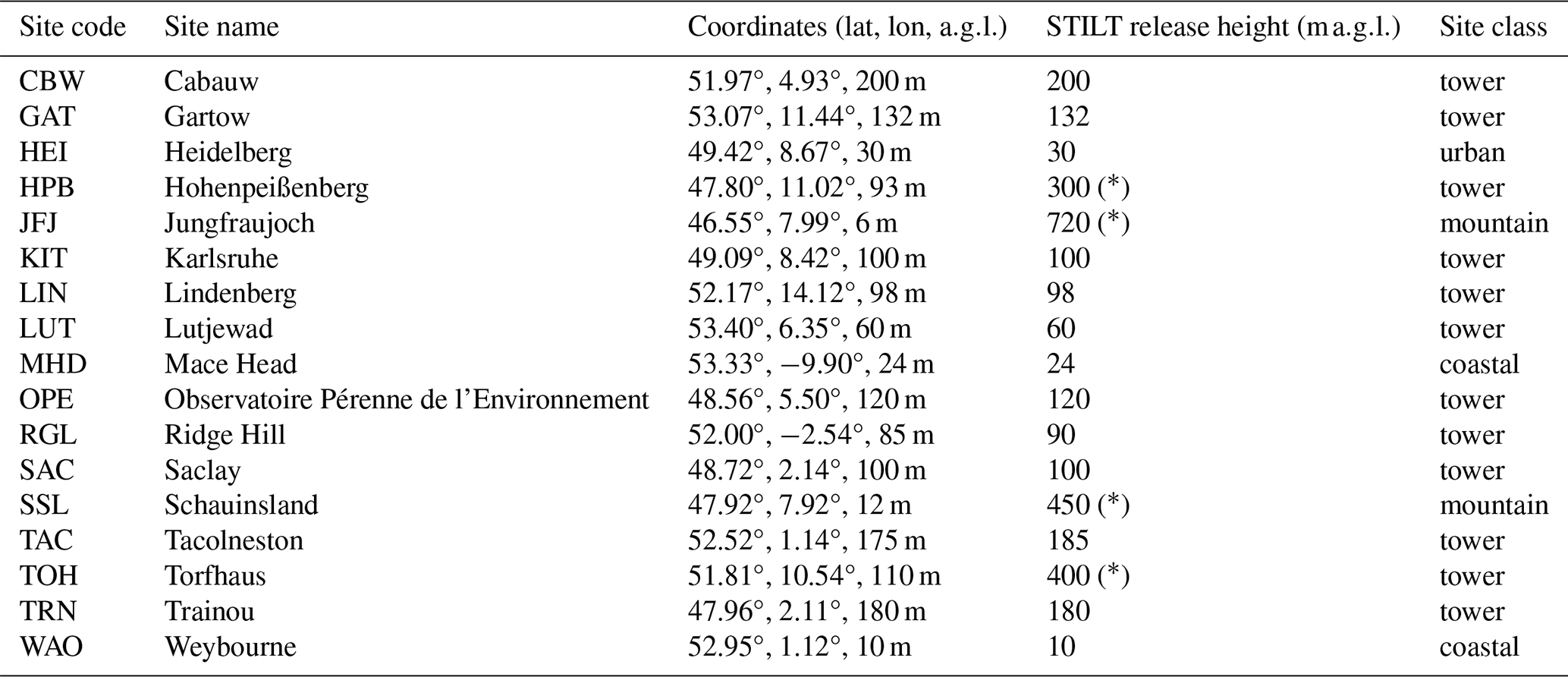
Table 1 Overview of the observation sites. For some high-altitude sites, marked with (^∗), a correction height was used to account for the steep terrain, which is hard to represent in the transport model.

2 Methods

2.1 CH₄ and Rn model-data mismatch

Before explaining the setup of the CH₄-Rn inversion, we describe the CH₄ and Rn observations, the atmospheric transport model, and the prior fluxes used to calculate the prior CH₄ and Rn MDM.

2.1.1 Observations

We use simultaneous hourly CH₄ and Rn observations from 17 European sites in 2021, where both gases are measured. While CH₄ is monitored at numerous sites across Europe, Rn observations remain limited in spatial coverage. The observation sites used in this study cover mainly central Europe and are located in the British Isles, northern France, the Netherlands, Germany and Switzerland (see Fig. 1). Most sites (12 out of 17) are continental tower stations, but there are also two coastal sites, two mountain sites and one urban site (see Table 1). To avoid atmospheric situations that are hard to represent with the transport model, we use only afternoon observations (11:00–16:00 UTC, except for the mountain sites), when the boundary layer is expected to be well mixed. In the case of the mountain sites, we use only night-time observations (23:00–04:00 UTC), when the impact of thermally induced winds is expected to be negligible. The CH₄ observations are from the Integrated Carbon Observation System Observation Package (ICOS-ObsPack, ICOS RI et al., 2024) data product and the Rn observations are described in Maier et al. (2025), hereafter referred to as “M25”. As in M25, we apply the calibration scale from the Heidelberg Radon Monitor (HRM) to all Rn observations. However, in Sect. 3.3, we further investigate the effect of using the alternative calibration scale from the Australian Nuclear Science and Technology Organisation (ANSTO), which results in ca. 11 % higher Rn activity concentrations (Schmithüsen et al., 2017). Note that we only use data for the hours when both CH₄ and Rn observations are available.

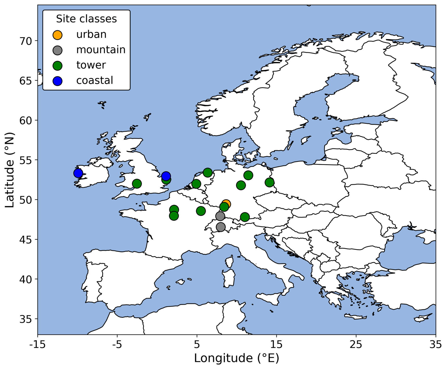
Figure 1 European model domain and observation sites. The colours of the symbols indicate the type of the observation sites.

2.1.2 Atmospheric transport model

We use the Stochastic Time-Inverted Lagrangian Transport model (STILT, Lin et al., 2003) to simulate hourly CH₄ and Rn concentrations at the 17 observation sites. STILT is driven with meteorological fields from the Integrated Forecasting System (IFS) of the European Centre for Medium-Range Weather Forecasts (ECMWF), extracted at a horizontal resolution of 0.25° and a temporal resolution of 3 h. As is typical for Lagrangian transport models, STILT calculates the surface influences (or so-called footprints) for each observation site by releasing 100 numerical particles per hour and transporting these particles backwards in time for 10 d (or until they leave the European model domain, see Fig. 1). The STILT footprints with unit $\mathrm{ppm}(\mathrm{\mu }\mathrm{mol}{\mathrm{m}}^{-\mathrm{2}}{\mathrm{s}}^{-\mathrm{1}}{)}^{-\mathrm{1}}$ describe the sensitivity of the observation sites to the upwind surface fluxes (with unit $\mathrm{\mu }\mathrm{mol}{\mathrm{m}}^{-\mathrm{2}}{\mathrm{s}}^{-\mathrm{1}}$), and the mapping of the footprints with the corresponding surface fluxes gives the CH₄ and Rn concentration contribution from fluxes within the model domain at each site. For Rn, we take into account its radioactive decay with a half-life of 3.8 d (see M25).

Table 2 Overview of the CH₄ and Rn prior fluxes.

^a Uncertainty in the annual total flux for the full European model domain [for Germany only]. ^b For regions outside Germany the same Rn fluxes based on the K15 model with GLDAS soil moisture are used.

2.1.3 Prior fluxes

Table 2 provides an overview of the CH₄ and Rn prior fluxes used in this study. We aggregated the CH₄ fluxes into four emission sectors: (1) anthropogenic emissions from agriculture and waste management; (2) anthropogenic emissions from land-based fossil fuel use; (3) natural fluxes from peatlands, mineral soils, inundated lands, wildfires, freshwaters, geological sources, and termites; and (4) oceanic emissions, including both anthropogenic contributions from fossil fuel exploitation and use, and natural sources. For the anthropogenic CH₄ emissions, we use the regional anthropogenic emission inventory from the Copernicus Atmosphere Monitoring Service (CAMS-REG-ANT, Kuenen et al., 2022). It covers emissions in Europe for the main air pollutants and GHGs. We use the latest version of the dataset, CAMS-REG-ANT-v8.1. The emission inventory uses official reported emission data to the United Nations Framework Convention on Climate Change (UNFCCC) to the extent possible. Where needed, due to data gaps or inconsistencies, reported data from selected countries were replaced or completed using other emission data. The data have been spatially distributed using proxy datasets developed by the Netherlands Organisation for Applied Scientific Research (TNO). Further details can be found in Denier van der Gon et al. (2025) and Kuenen et al. (2022). For use in the inversion, all CH₄ fluxes are aggregated to a monthly temporal resolution and re-gridded to a common spatial resolution of 0.25° × 0.25°.

For the Rn prior flux, we use a daily-resolution, process-based Rn flux map developed in M25, which is based on the Rn flux model from Karstens et al. (2015), hereafter referred to as the “K15 model”. High-resolution (1 km × 1 km) soil moisture data from the German Weather Service (DWD) are used for Germany, while coarser-resolution (0.25° × 0.25°) soil moisture data from GLDAS-Noah (Beaudoing and Rodell, 2020) are employed for the rest of Europe. The soil moisture data used to simulate the diffusive Rn transport in the soil represents the average over the top 10 cm of the soil column. In M25, we demonstrated that using the top 10 cm average soil moisture – rather than the top 40 cm or top 100 cm – leads to better agreement between the temporal variability of the process-based Rn fluxes and the posterior flux estimate from a flat-prior Rn inversion (where prior fluxes are spatially and temporally constant). In Sect. 3.3, we evaluate the sensitivity of the CH₄ flux estimates from the dual-tracer inversion to potential biases in the Rn prior flux. To do so, we analyse the CH₄ flux estimates for Germany, a region well-covered by the observational sites. For this purpose, we construct two alternative Rn flux maps for Germany: (1) using the K15 model again, but this time with coarse (0.25° × 0.25°) GLDAS-Noah soil moisture data (top 10 cm) over Germany; and (2) using the LandscapeDNDC model (Haas et al., 2013), a process-based framework designed to simulate ecosystem-atmosphere exchanges, primarily for carbon and nitrogen cycling. To apply LandscapeDNDC to Rn flux simulation, we implement the same radium source and Rn emanation parameterization as in the K15 model. However, LandscapeDNDC explicitly models both the soil water dynamics and the Rn transport in the top 2 m of soil, including diffusion, advection, dissolution and leaching processes within and between 34 soil layers. We run separate simulations for agricultural soils and forests, and calculate combined Rn fluxes as area-weighted averages using the Corine Landcover (2018) data. For regions outside Germany, we use the same Rn fluxes for all three scenarios, namely the fluxes derived from the K15 model and GLDAS-Noah soil moisture data (top 10 cm). All Rn flux maps have a daily temporal resolution and are re-gridded to a spatial resolution of 0.25° × 0.25°.

Figure 2 Three different Rn flux estimates for Germany in 2021. The Rn fluxes were calculated using the K15 model with GLDAS-Noah (red) and DWD (yellow) soil moisture, and the LandscapeDNDC model (blue).

Figure 2 compares the three Rn flux estimates for Germany. The flux derived using coarse-resolution GLDAS-Noah soil moisture data (red curve) exhibits the lowest temporal variability and the highest annual mean value. In contrast, both the high-resolution LandscapeDNDC model (blue curve) and the K15 model combined with high-resolution DWD soil moisture data (yellow curve) produce fluxes with greater temporal variability. Among these, the LandscapeDNDC-based flux is slightly lower than that from the K15 model. In our standard inversion configuration, we use the Rn flux from the K15 model driven by high-resolution DWD soil moisture data as prior estimate, which lies between the GLDAS-based and the LandscapeDNDC-based fluxes. The two other Rn flux maps are used in additional inversion runs to investigate the impact of the Rn prior flux on the CH₄ flux estimates in the dual-tracer approach (see Sect. 3.3).

2.1.4 Boundary conditions

Since we perform a regional inversion in Europe, we need lateral boundary conditions. For CH₄, we use the global inversion optimized CH₄ concentration field from the Copernicus Atmosphere Monitoring Service (CAMS) based on surface observations (v24r1, CAMS, 2020a; Bergamaschi et al., 2013). For Rn, we use the CAMS global reanalysis (EAC4) Rn concentration field (CAMS, 2020b; Inness et al., 2019). The CH₄ and Rn concentrations in the grid cells where the STILT back-trajectories end or leave the European domain (see Fig. 1) determine the CH₄ and Rn background concentrations, which we subtracted from the CH₄ and Rn observations. For Rn, we account for its radioactive decay during transport from the boundary cells to the observation sites. CH₄ has an atmospheric sink, primarily through reaction with hydroxyl radicals (OH), resulting in an average atmospheric lifetime of approximately 9 years (Saunois et al., 2025). We incorporate this lifetime by assuming a constant decay rate when transporting boundary conditions to the observation sites (note that we neglect this atmospheric CH₄ sink when transporting fluxes within the footprint to the observation sites, as the relevant timescales are typically much shorter). The CH₄ and Rn MDM used to constrain the respective fluxes in the European model domain is calculated by subtracting the modelled CH₄ and Rn concentrations from the CH₄ and Rn observations (after background subtraction).

2.1.5 Outlier flagging

To avoid the inversion results being too heavily influenced by periods with a high MDM that cannot be represented by the transport model, we performed a so-called σ-screening, as suggested by Rödenbeck et al. (2018). For this, we conducted 17 separate CH₄ and Rn single-tracer inversion runs, excluding each time a different one of the 17 sites (so-called “leave-one-out” runs). The setup of these pre-inversions is described in more detail in Appendix A. The resulting posterior fluxes are then used to calculate the hourly CH₄ and Rn posterior MDM at the excluded sites. For each site, we disregard all CH₄ and Rn data, for which the absolute value of either the posterior CH₄ MDM or the posterior Rn MDM was outside the respective 3σ-range, i.e. was larger than 3 times the standard deviation of the hourly posterior CH₄ and Rn MDM, respectively. By excluding the CH₄ and Rn MDM outliers from both data sets, we ensure that the final 3σ-screened data sets contain CH₄ and Rn observations for the same hours. We use these 3σ-screened CH₄ and Rn data sets as the observational input for both the single- and dual-tracer inversions, which are described in the following section.

2.2 Setup of the CH₄-Rn inversion

In the following we describe the inversion framework, the setup of the single-tracer CH₄-only and Rn-only inversions, and the extension of the inversion system to use dual tracers.

2.2.1 Inversion framework

We use the CarboScope-Regional inversion system described in Rödenbeck et al. (2003, 2009). It uses a Bayesian framework to estimate daily fluxes for each grid cell in the European model domain (see Fig. 1). The inversion algorithm and the iterative approach for minimising the Bayesian cost function are explained in detail in the technical report by Rödenbeck (2005) using the example of a CO₂ flux inversion. Therefore, our focus here is on the specifics of the CH₄ and Rn inversions.

A Bayesian cost function J can be written in the following form:

$$\begin{array}{}\text{(1)}& \begin{array}{rl}J\left(\mathit{x}\right)=& (\mathit{y}-H(\mathit{x}\left){)}^{\mathrm{T}}{\mathbf{Q}}_{\mathrm{m}}^{-\mathrm{1}}\right(\mathit{y}-H\left(\mathit{x}\right))\\ & +(\mathit{x}-{\mathit{x}}_{\mathrm{p}}{)}^{\mathrm{T}}{\mathbf{Q}}_{\mathrm{p}}^{-\mathrm{1}}(\mathit{x}-{\mathit{x}}_{\mathrm{p}})\end{array}\end{array}$$

The first term on the right-hand side of Eq. (1) describes the data constraint, and the second term includes the prior flux information (note that the second term in Eq. 1 is written in a slightly different form in the CarboScope framework, cf. Eq. 14 in Rödenbeck, 2005). The state vector x contains the daily CH₄ and Rn fluxes of each grid cell, the observed CH₄ and Rn concentrations (after background subtraction and outlier flagging) are in y, and the modelled CH₄ and Rn concentrations are described by H(x). Minimising J(x) means that the CH₄ and Rn MDM, i.e. (y−H(x)), is minimised by adjusting the CH₄ and Rn fluxes in x, and taking into account the MDM uncertainties described by the MDM error covariance matrix Q_m and the CH₄ and Rn prior flux information (the vector x_p contains the CH₄ and Rn prior fluxes, and Q_p is the prior error covariance matrix). For CH₄, each of the four prior flux sectors shown in Table 2 is adjusted individually; however, we mainly focus on the total CH₄ flux in this study to avoid the risk that the inversion cannot distinguish between sectors when they are not spatially separated.

2.2.2 Uncertainties

The diagonal elements of the MDM error covariance matrix Q_m contain the combined uncertainties of the observations and the transport model for CH₄ and Rn, respectively. To estimate these MDM uncertainties for each site, we use again the “leave-one-out” (LOO) runs, which are described in more detail in Appendix A. We calculate the CH₄ and Rn concentrations at each site using the posterior flux estimate of the corresponding LOO run, which is not constrained by observations from that site. We refer to these posterior concentrations at the excluded site obtained using the corresponding LOO posterior flux as the LOO-based concentrations, and we compare them with the respective observations. The (annual) mean difference between the LOO-based concentrations and the observed concentrations may predominantly be affected by potential biases in the fluxes around the excluded site. This is because these fluxes were not constrained by observations from the excluded site in the LOO runs. Furthermore, we assume that the temporal variability in the difference between the LOO-based concentrations and the observed concentrations is primarily caused by shortcomings in how the transport model represents the observations from the excluded site. This assumption may be justified for CH₄ and Rn, for which we do not expect large temporal variability in the fluxes not resolved in the prior. Therefore, we use the standard deviation of the difference between the LOO-based concentrations and the observed concentrations as a measure of the MDM uncertainty at the excluded site. As we use outlier-screened data in the inversion (see Sect. 2.1.5), we calculate the standard deviation of the difference between the LOO-based concentrations and the observed concentrations using the outlier-flagged CH₄ and Rn data sets. The estimated MDM uncertainty ranges between 16 and 46 ppb for CH₄ and between 0.4 and 1.5 Bq m⁻³ for Rn at the individual sites (see Fig. A1). Note that we conducted the LOO runs only once, separately for the CH₄-only and the Rn-only inversions, using the standard prior uncertainty settings specified in Table 2. The resulting MDM uncertainty estimates were then used for all dual-tracer and single-tracer inversion runs.

For the single-tracer inversions, where only CH₄ or Rn fluxes are optimized, the cost function (and thus Q_m) consists of only one tracer and the off-diagonal elements of Q_m are assumed to be zero. However, to account for temporal correlations between the MDM of the same tracer during consecutive hours within a week (i.e. the typical time scale of synoptic circulation), we applied a so-called data density weighting, which increases the MDM uncertainty of hourly measurements by the square root of the number of observations within a week (see Rödenbeck, 2005, Kountouris et al., 2018). Note that we assumed the same MDM uncertainty estimates in the diagonal elements of Q_m for the dual- and single-tracer inversions.

For each of the CH₄ prior emission sectors and the Rn prior fluxes, we assume an uncertainty of 30 % for the annual total flux of the European model domain. This corresponds to roughly 60 % uncertainty for the annual total flux of Germany, for both the CH₄ sectors and Rn (see Table 2). The chosen uncertainty for the CH₄ prior flux is in the range of the values used in the CH₄ inversion intercomparison study by Ioannidis et al. (2026; see their Table 3). To investigate the impact of uncertainties in the Rn prior flux on the derived CH₄ flux estimates in the dual-tracer approach, we conduct a series of sensitivity runs in which the Rn prior flux uncertainty is varied between (unrealistic) 5 % and 200 % for the annual total flux of Germany. We assume exponentially decaying spatial correlations between the prior flux errors in the grid cells and choose a spatial correlation length of ca. 300 km for both tracers. We also assume a temporal correlation length of 1 month for CH₄ and 3.5 d for Rn (“Filt6T” and “Filt52T”, respectively, in CarboScope notation, see Rödenbeck, 2005) and neglect potential correlations between the prior flux errors of the individual CH₄ sectors.

2.2.3 Extensions for the dual-tracer CH₄-Rn inversion

As mentioned above, for single-tracer CH₄-only and Rn-only inversions, we assume that the MDM error covariance has a diagonal form, which is easy to invert. However, in case of the dual-tracer inversion, correlations between the CH₄ and Rn MDM must be taken into account, making the MDM error covariance matrix non-diagonal. In our implementation, the MDM error covariance matrix Q_m of the dual-tracer CH₄-Rn inversion has the following form:

$$\begin{array}{}\text{(2)}& {\mathbf{Q}}_{\mathrm{m}}=\left(\begin{array}{ccccccc}{\mathit{\sigma }}_{{\mathrm{CH}}_{\mathrm{4}},t_{\mathrm{1}}}^{\mathrm{2}}& {\text{cov}}_{t_{\mathrm{1}}}& \mathrm{0}& \mathrm{0}& \mathrm{\cdots }& \mathrm{0}& \mathrm{0}\\ {\text{cov}}_{t_{\mathrm{1}}}& {\mathit{\sigma }}_{\mathrm{Rn},t_{\mathrm{1}}}^{\mathrm{2}}& \mathrm{0}& \mathrm{0}& \mathrm{\cdots }& \mathrm{0}& \mathrm{0}\\ \mathrm{0}& \mathrm{0}& {\mathit{\sigma }}_{{\mathrm{CH}}_{\mathrm{4}},t_{\mathrm{2}}}^{\mathrm{2}}& {\text{cov}}_{t_{\mathrm{2}}}& \mathrm{\cdots }& \mathrm{0}& \mathrm{0}\\ \mathrm{0}& \mathrm{0}& {\text{cov}}_{t_{\mathrm{2}}}& {\mathit{\sigma }}_{\mathrm{Rn},t_{\mathrm{2}}}^{\mathrm{2}}& \mathrm{\cdots }& \mathrm{0}& \mathrm{0}\\ \mathrm{0}& \mathrm{0}& \mathrm{0}& \mathrm{0}& \mathrm{\cdots }& \mathrm{0}& \mathrm{0}\\ \mathrm{\cdots }& \mathrm{\cdots }& \mathrm{\cdots }& \mathrm{\cdots }& \mathrm{\cdots }& {\mathit{\sigma }}_{{\mathrm{CH}}_{\mathrm{4}},t_n}^{\mathrm{2}}& {\text{cov}}_{t_n}\\ \mathrm{0}& \mathrm{0}& \mathrm{0}& \mathrm{0}& \mathrm{\cdots }& {\text{cov}}_{t_n}& {\mathit{\sigma }}_{\mathrm{Rn},t_n}^{\mathrm{2}}\end{array}\right)\end{array}$$

with ${\mathit{\sigma }}_{{\mathrm{CH}}_{\mathrm{4}},t_i}^{\mathrm{2}}$ and ${\mathit{\sigma }}_{\mathrm{Rn},t_i}^{\mathrm{2}}$ being the variances of the CH₄ and Rn MDM, and ${\text{cov}}_{t_i}$ being the covariance of the CH₄ and Rn MDM for time t_i, respectively. Q_m is a block diagonal matrix of the form:

$$\begin{array}{}\text{(3)}& {\mathbf{Q}}_{\mathrm{m}}=\left(\begin{array}{cccc}{\mathbf{A}}_{t_{\mathrm{1}}}& \mathrm{0}& \mathrm{\cdots }& \mathrm{0}\\ \mathrm{0}& {\mathbf{A}}_{t_{\mathrm{2}}}& \mathrm{\cdots }& \mathrm{0}\\ \mathrm{\cdots }& \mathrm{\cdots }& \mathrm{\cdots }& \mathrm{\cdots }\\ \mathrm{0}& \mathrm{0}& \mathrm{\cdots }& {\mathbf{A}}_{t_n}\end{array}\right)\end{array}$$

with

$$\begin{array}{}\text{(4)}& {\mathbf{A}}_{t_i}=\left(\begin{array}{cc}{\mathit{\sigma }}_{{\mathrm{CH}}_{\mathrm{4}},t_i}^{\mathrm{2}}& {\text{cov}}_{t_i}\\ {\text{cov}}_{t_i}& {\mathit{\sigma }}_{\mathrm{Rn},t_i}^{\mathrm{2}}\end{array}\right)\end{array}$$

The MDM error covariance matrix Q_m is invertible if the individual matrices ${\mathbf{A}}_{t_i}$ are invertible, i.e. if:

$$\begin{array}{}\text{(5)}& \text{det}\left({\mathbf{A}}_{t_i}\right)={\mathit{\sigma }}_{{\mathrm{CH}}_{\mathrm{4}},t_i}^{\mathrm{2}}{\mathit{\sigma }}_{\mathrm{Rn},t_i}^{\mathrm{2}}-{\text{cov}}_{t_i}{\text{cov}}_{t_i}\ne \mathrm{0}\end{array}$$

The inverse of Q_m can then be written as:

$$\begin{array}{}\text{(6)}& {\mathbf{Q}}_{\mathrm{m}}^{-\mathrm{1}}=\left(\begin{array}{cccc}{\mathbf{A}}_{t_{\mathrm{1}}}^{-\mathrm{1}}& \mathrm{0}& \mathrm{\cdots }& \mathrm{0}\\ \mathrm{0}& {\mathbf{A}}_{t_{\mathrm{2}}}^{-\mathrm{1}}& \mathrm{\cdots }& \mathrm{0}\\ \mathrm{\cdots }& \mathrm{\cdots }& \mathrm{\cdots }& \mathrm{\cdots }\\ \mathrm{0}& \mathrm{0}& \mathrm{\cdots }& {\mathbf{A}}_{t_n}^{-\mathrm{1}}\end{array}\right)\end{array}$$

with

$$\begin{array}{}\text{(7)}& {\mathbf{A}}_{t_i}^{-\mathrm{1}}={\displaystyle \frac{\mathrm{1}}{\text{det}\left({\mathbf{A}}_{t_i}\right)}}\left(\begin{array}{cc}{\mathit{\sigma }}_{\mathrm{Rn},t_i}^{\mathrm{2}}& -{\text{cov}}_{t_i}\\ -{\text{cov}}_{t_i}& {\mathit{\sigma }}_{{\mathrm{CH}}_{\mathrm{4}},t_i}^{\mathrm{2}}\end{array}\right)\end{array}$$

In our current setup, we assume that the CH₄-Rn MDM correlation coefficients are the same for each site and do not change over time, i.e. ${\mathbf{A}}_{t_i}=\mathbf{A}$ (note that if the number of observations varies from week to week, the ${\mathbf{A}}_{t_i}$ can also change over time due to the so-called data density weighting, see Sect. 2.2.2). This means that we can directly calculate the inverse of the MDM error covariance matrix Q_m if ${\mathit{\sigma }}_{{\mathrm{CH}}_{\mathrm{4}}}^{\mathrm{2}}{\mathit{\sigma }}_{\mathrm{Rn}}^{\mathrm{2}}\ne {\text{cov}}^{\mathrm{2}}$, i.e. if the CH₄-Rn MDM correlation coefficient $r_{\text{MDM}}=\text{cov}/\left({\mathit{\sigma }}_{{\mathrm{CH}}_{\mathrm{4}}}{\mathit{\sigma }}_{\mathrm{Rn}}\right)\ne \mathrm{1}$. In Sect. 3.1 we will investigate the spatial and temporal variability of the CH₄-Rn MDM correlation and we will further investigate the influence of the MDM correlation coefficient on the dual-tracer inversion results in Sect. 3.3. In our standard configuration, we use the same constant MDM correlation coefficient of 0.6 for all sites and all times, which is the median correlation coefficient for the 17 observation sites (see Fig. S1 in the Supplement). We further assume that the errors in the CH₄ and Rn prior fluxes are uncorrelated. We discuss this assumption in Sect. 3.1.2. The results of the single-tracer and dual-tracer inversions are compared in Sect. 3.2. To evaluate their performance, we investigate the so-called uncertainty reduction (UR), which is defined as the deviation of the ratio between the posterior and prior flux uncertainties from 1. A higher UR indicates a greater reduction in posterior flux uncertainty relative to the assumed prior flux uncertainty.

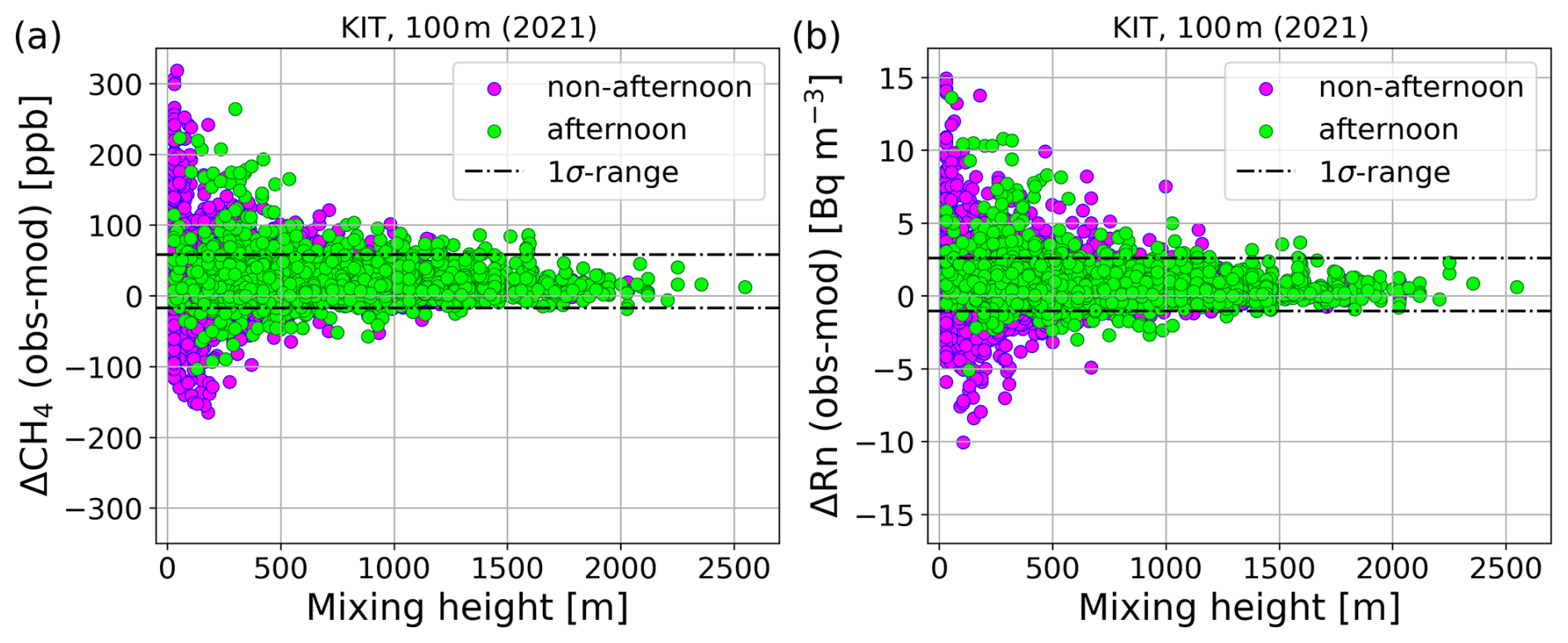
Figure 3 Hourly CH₄ (a) and Rn (b) MDM in dependence of the modelled mixing height from STILT for the Karlsruhe (KIT) tower site at 100 $\mathrm{m}\mathrm{a}.\mathrm{g}.\mathrm{l}.$ Afternoon (11:00–16:00 UTC) data and non-afternoon data are shown in green and magenta, respectively. The standard deviation (1σ-range) of the CH₄ and Rn MDM (afternoon and non-afternoon data) is indicated by the dashed black lines.

3 Results and Discussion

3.1 Transport model performance and CH₄-Rn MDM correlation

3.1.1 Dependence of transport model performance on mixing height

To motivate the use of Rn in a dual-tracer inversion, we first investigate how the performance of the transport model depends on the planetary boundary layer height (PBLH). Figure 3 shows the hourly CH₄ and Rn MDM as a function of the modelled mixing height, using the continental Karlsruhe (100 m) tower site as an example (see Fig. S2 for the other sites). During stable atmospheric conditions, characterised by low mixing heights, both the CH₄ and Rn MDM variability is significantly larger than during well mixed atmospheric conditions with high mixing heights. The standard deviation of the CH₄ and Rn MDM is for mixing heights below 500 m about twice as large as for mixing heights above 500 m. Low mixing heights occur mainly at night, when the surface cools and a stable nocturnal boundary layer is formed. Therefore, typically only afternoon observations are used in inversion studies to account for the inability of transport models to adequately represent the build-up and break-down of the nocturnal boundary layer (e.g., Monteil et al., 2020). However, there are also stable afternoon situations with low mixing heights, mainly in winter (see green points in Fig. 3). At the Karlsruhe site, around a quarter of the afternoon observations are associated with mixing heights < 500 m, and the standard deviation of the CH₄ (and Rn) MDM of the afternoon observations is even 134 % (and 144 %) larger for mixing heights < 500 m than for mixing heights > 500 m. Averaged over all 17 sites, 33 % of the afternoon observations were made during stable conditions (PBLH < 500 m), and the standard deviation of the afternoon CH₄ (and Rn) MDM is 105 % (and 128 %) larger during stable (PBLH < 500 m) than during well-mixed (PBLH > 500 m) conditions (see Fig. S2). The two coastal sites Weybourne and Mace Head show the largest differences (over 200 %) in the afternoon model performance between low and high mixing height conditions (Fig. S2a and c). The strongly negative CH₄ and Rn MDM during low mixing heights indicates that vertical mixing is underestimated under stable conditions near the coast. Moreover, since both the natural CH₄ and Rn sources in the ocean are minor to negligible, respectively, a strong negative MDM at a coastal site could be attributed not only to a bias in the simulated vertical mixing but also to inaccuracies in the modelled wind direction. Specifically, if the model's back-trajectories suggest contributions of CH₄ and Rn from land areas, while the measurements indicate clean air conditions from the ocean. In contrast, the high-altitude mountain site Jungfraujoch (3572 m) shows even a slightly better model performance for low mixing heights than for high mixing heights (Fig. S2k). This could be explained by the fact that the Jungfraujoch site is in the free troposphere during low mixing height conditions, and is thus during those events less affected by local sources within the boundary layer. In addition, during nighttime there are generally no thermal upwinds along the slopes that would transport emissions from local sources towards mountain stations.

Although it is well known that the transport model performance depends on atmospheric conditions (e.g., Gerbig et al., 2008), inversion studies often assume temporally constant transport model errors due to lack of information to separate the effect of transport model errors from the effect of potential biases in the prior fluxes on the MDM variability. Such time-constant model errors may overestimate the true errors during atmospheric conditions with high mixing heights and underestimate the errors during low mixing height conditions. As a result, the observations during low mixing height conditions, which are difficult to represent with the model, are relatively over-weighted in the inversion compared to observations during well-mixed situations, which are typically easier to describe. This could lead to biases in the top-down flux estimates. To (partially) overcome this, some studies applied an additional outlier removal to the afternoon data (e.g., Rödenbeck et al., 2018; Lu et al., 2021). Recently, some studies use time-varying transport model uncertainties, e.g. as a function of local wind speed (Bergamaschi et al., 2022) or by running (computationally demanding) meteorological ensembles (e.g., Steiner et al., 2024; Bruch et al., 2025). In our study, we use the additional information from Rn and exploit the similarity in the CH₄ and Rn MDM variability to better represent the transport model error in the inversion system. In the following, we investigate the correlation between the CH₄ and Rn MDM in more detail and discuss why possible correlations in the CH₄ and Rn prior fluxes might be negligible at sites in central Europe.

3.1.2 Correlation between the CH₄ and Rn MDM

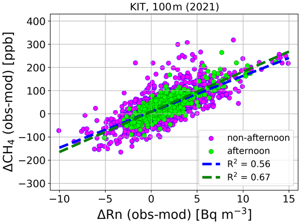
Figure 4 shows the correlation between the hourly CH₄ and Rn MDM for the Karlsruhe (100 m) tower site. The Pearson's correlation coefficient r is 0.82 (R² = 0.67) for afternoon data (r=0.75 for non-afternoon data) with a slightly higher value in the winter half-year (r=0.79) compared to the summer half-year (r=0.71). In principle, this correlation can be explained by errors in the transport model, which affect both the CH₄ and Rn simulations, as well as by correlated errors in the CH₄ and Rn prior fluxes. However, we expect potential correlations in the errors of the CH₄ and Rn prior fluxes to be small at sites in central Europe that are mainly influenced by anthropogenic CH₄ emissions, which have a different origin than the Rn fluxes. Note that in the central European domain (45–55° N, 10° W–15° E), which encompasses all observation sites, anthropogenic CH₄ emissions account for ca. 80 % of the total CH₄ flux. The situation might be different at sites, which are substantially influenced by soil moisture-driven CH₄ fluxes, such as from peatlands or organic soils. However, while an increased soil water content typically reduces Rn exhalation due to suppressed gas diffusion in the soil, it is expected to enhance CH₄ emissions from peatlands by limiting oxygen availability and promoting anaerobic microbial activity (Song et al., 2021). Therefore, we would expect that the errors in the peatland CH₄ emissions and the Rn fluxes are rather anti-correlated. Soil moisture also affects CH₄ uptake by altering oxygen diffusion and microbial processes in the soil (Lohila et al., 2016). However, given that CH₄ fluxes from peatlands and organic soils account for less than 2 % of total CH₄ emissions within the central European domain, we do not expect a significant correlation in the errors of the CH₄ and Rn fluxes at the sites used in this study. Hence, we assume that the correlation between the CH₄ and Rn MDM is mainly due to errors in the transport model; and an R² value greater than 0.5 would mean that more than 50 % of the variability in the CH₄ MDM can be attributed to errors in the transport model.

Figure 4 Correlation between the hourly CH₄ and Rn MDM for afternoon (green) and non-afternoon (magenta) observations from the Karlsruhe (KIT) tower site in 2021. The green and blue dashed lines indicate linear fits through the respective data.

To further support this hypothesis, we investigate for the exemplary Karlsruhe site how the correlations between the CH₄ and Rn MDM would change if we used a different transport model (the FLEXible PARTicle dispersion model (FLEXPART; Stohl et al., 2005; Pisso et al., 2019) and the Numerical Atmospheric-dispersion Modelling Environment (NAME; Jones et al., 2007) instead of STILT) for the Rn simulations. To do this, we use the FLEXPART and NAME Rn simulations from M25. Importantly, the corresponding CH₄ simulations are still performed with STILT. It turns out that the correlations become worse when the Rn concentrations are modelled with a different transport model than the CH₄ concentrations: the R² values of the afternoon data decrease to 0.44 and 0.34 when comparing the STILT-based CH₄ MDM with the FLEXPART and NAME-based Rn MDM, respectively (see Fig. S3). This shows that the errors in STILT are only slightly correlated with the errors in FLEXPART and NAME, respectively. Moreover, it illustrates that potential correlations in the errors of the CH₄ and Rn prior fluxes would lead to a much smaller correlation in the CH₄ and Rn MDM than common errors in the transport model.

Overall, this analysis elucidates that most of the correlation between the CH₄ and Rn MDM can be explained by errors in the transport model. Figure S1 presents the CH₄-Rn MDM correlation coefficients for all 17 sites. The sites with the strongest MDM correlations are coastal and continental tower sites, where the variability of the CH₄ MDM is mainly due to model deficits in describing vertical mixing. At coastal sites, part of the MDM correlation could also be attributed to the fact that both the CH₄ and Rn fluxes, and consequently their (absolute) errors, are relatively small over the ocean. The weakest MDM correlation is found at Lutjewaad, which is strongly influenced by local CH₄ emissions leading to sharp spikes in the CH₄ concentration that is difficult to represent with a coarse-resolution model. The median of the 17 CH₄-Rn MDM correlation coefficients is ca. 0.6. We apply this (constant) median value in the formulation of the MDM covariance matrix to link the CH₄ and the Rn information in the dual-tracer inversion (see Sect. 2.2.3). Before analysing the results of the CH₄-Rn inversion in Sect. 3.2.2, we present the results of two separate single-tracer CH₄-only and Rn-only inversions.

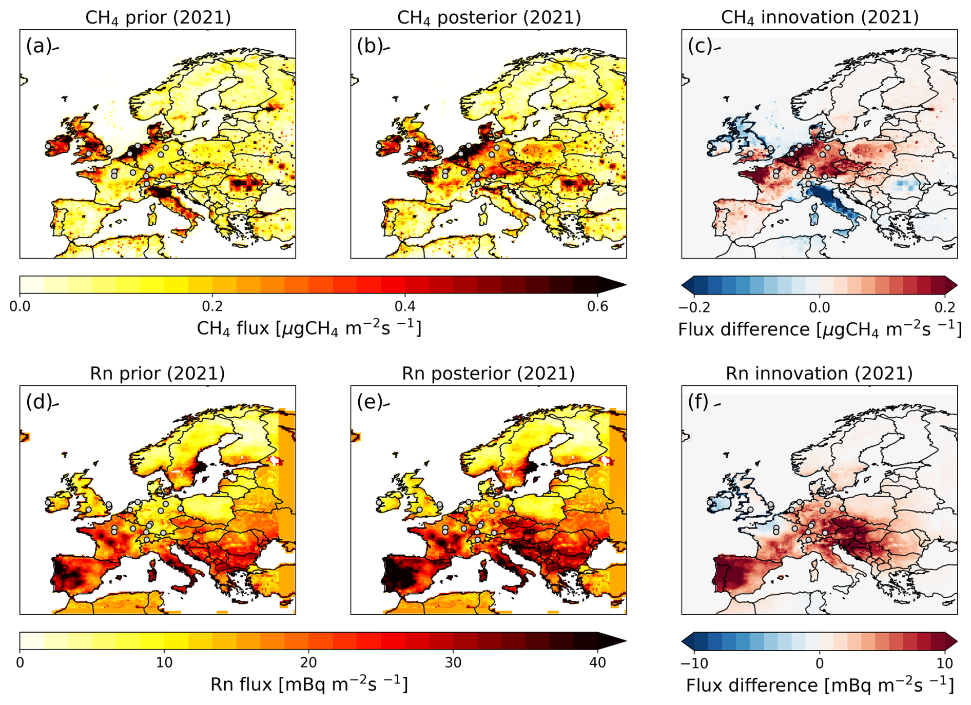
Figure 5 CH₄ (a, b) and Rn (d, e) emission maps for the prior (a, d) and posterior (b, e) fluxes in 2021, and maps for the CH₄ (c) and Rn (f) innovation (i.e. the posterior minus prior flux differences). Shown are the results from the single-tracer inversions.

Figure 6 Daily prior (black) and posterior CH₄ (a) and Rn (b) fluxes of the single-tracer inversions (red) and the dual-tracer inversion (blue) for Germany in 2021. The dark blue curves represent the dual-tracer inversion results assuming the same relative uncertainty (i.e. roughly 60 % for the annual total flux in Germany) for both CH₄ and Rn prior fluxes. The light-blue curves show the dual-tracer inversion results for reduced Rn prior flux uncertainties, ranging from 30 % to (unrealistic) 5 %.

3.2 Comparison of dual-tracer with single-tracer inversion results

3.2.1 Single-tracer inversion results

At most of the continental sites the model underestimates the observed CH₄ and Rn concentrations when using prior fluxes (see Fig. S4). As a consequence, the single-tracer CH₄-only and Rn-only inversions increase the fluxes in central Europe to reduce the MDM at the stations. In the case of CH₄, the largest positive innovation (posterior minus prior flux difference) is found in north-west and south-east Germany, the Netherlands, Belgium, and north-west France, where prior fluxes are also high (see Fig. 5a–c). In contrast, CH₄ fluxes are strongly reduced in Italy, especially natural emissions (not shown). This may be attributed to overestimated geological prior fluxes, which are substantial in this region (see Ioannidis et al., 2026). However, Italy is not covered by the observational sites used in this study and is therefore not well constrained by our inversion (see Fig. S9). In Germany, the annual total CH₄ emissions are increased by 75 % compared to the prior flux estimate (see red curve in Fig. 6a). Moreover, the posterior CH₄ flux in Germany shows a strong seasonal cycle, with minima in April and November, and a maximum in September. This seasonal cycle is mainly data-driven, as the seasonal variations in the prior flux are small, although a maximum around September is also present in the prior (see black curve in Fig. 6a). Additional CH₄-only inversion runs based on different uncertainty settings and station sets confirm the robustness of the CH₄ flux estimate for Germany and its seasonal variation (see Figs. S5 and A2c). As each CH₄ flux sector is adjusted individually by the inversion (see Sect. 2.2), we can investigate, which sector is responsible for the seasonal cycle in the total CH₄ flux estimate for Germany (see Fig. S6). Since we have applied the same relative prior flux uncertainty for each sector, the inversion mainly adjusts the by far largest CH₄ sector (i.e., the agriculture and waste sector) with the largest absolute uncertainty (see Fig. S6b). However, even if we assume the same absolute uncertainty for each sector, so that the inversion has more flexibility to adjust the fluxes of the low-contributing sectors, the seasonal cycle of the (total) CH₄ flux is mainly determined by the agriculture and waste sector (see Fig. S6c). Therefore, we assume that the seasonal cycle in the CH₄ flux of Germany in 2021 is due to an interplay between emissions from the use of fossil fuels (which are expected to decrease in summer) and emissions from the agricultural sector (which are expected to increase during the grazing season; Tong et al., 2023). In their intercomparison study, Ioannidis et al. (2026) found a similar mean seasonal cycle in western Europe during the period 2006–2018. Hence, it may be interesting to investigate whether the seasonal pattern in our German CH₄ emission estimates is also present in other years.

In the case of Rn, fluxes are increased over much of central and southern Europe, but the strongest increases are in eastern Europe and on the Iberian Peninsula, i.e., in regions without observational constraints (cf. Fig. S9). In contrast, the Rn fluxes are slightly reduced over the British Isles and northern France. This could at least partly be explained by the on average negative difference between observed and modelled Rn concentrations at the sites on the British Isles (MHD, RGL, WAO, and TAC; see Fig. S4). In particular, MHD and WAO exhibit strong negative MDMs during stable atmospheric conditions with low mixing heights (see Fig. S2a and c). In Germany, the annual total Rn fluxes are increased by 45 % (see red curve in Fig. 6b).

Overall, the adjustment of the CH₄ and Rn fluxes leads to a median reduction of the MDM bias by 69 % and 58 %, respectively, at the observation sites. Moreover, the observational information leads to a strong uncertainty reduction of the flux estimates in central Europe (cf. Fig. 8c). The statistical uncertainty of the annual total posterior fluxes in Germany is 85 % lower for CH₄ and 88 % lower for Rn compared to the assumed uncertainty of the respective prior fluxes.

Figure 7 Maps showing the difference between the posterior flux of the dual-tracer inversion and the posterior flux of the corresponding single-tracer inversion for CH₄ (a) and Rn (b). The same relative uncertainty (30 % for the European total flux, which corresponds to roughly 60 % for the annual total flux in Germany) was assumed for the CH₄ and Rn prior fluxes. The colour bar scale limits represent 10 % (in a) and 20 % (in b) of the scale range shown in the innovation plots in Fig. 5c and f, respectively.

3.2.2 Dual-tracer inversion results

Figure 7 shows the difference between the posterior CH₄ and Rn flux of the dual-tracer inversion and the corresponding posterior flux of a single-tracer inversion. The relative differences are within 10 % for most of central Europe. However, the spatial pattern of the differences is different for CH₄ and Rn. Compared to the single-tracer inversion, the dual-tracer inversion results in lower Rn fluxes mainly in the southern part of the British Isles, northern France and Belgium, southern Sweden, and the Iberian Peninsula, while yielding higher Rn fluxes in Italy. In contrast, the dual-tracer inversion leads to lower CH₄ fluxes mainly over the British Isles, the Netherlands, south-eastern Germany, and northern Italy, and to higher CH₄ fluxes in northern Germany, Denmark, and Italy. Overall, the spatial pattern in Fig. 7a (and b) illustrates the impact of the Rn (and CH₄) observations on the CH₄ (and Rn) flux estimates in the dual-tracer approach.

Figure 8 Impact of Rn prior flux uncertainty (a, c) and MDM correlation coefficient (b, d) on CH₄ flux estimates from the dual-tracer inversion. Panels (a) and (b) show the ratio between posterior CH₄ fluxes from the dual-tracer and the single-tracer inversion for different Rn prior flux uncertainties (a) and for different MDM correlation coefficients (b). Panels (c) and (d) present the uncertainty reduction (UR) for CH₄ fluxes in the dual-tracer inversion across varying Rn prior uncertainties (c) and MDM correlation coefficients (d). For comparison, UR values for the CH₄ flux results from the single-tracer inversion are indicated in white boxes on the left side of panels (c) and (d). The uncertainty values for the Rn prior flux represent the uncertainty for the annual total flux of the full European model domain (they correspond to 5 % to 200 % uncertainty for the annual total flux of Germany). Results are shown for six countries: Belgium (BEL), Switzerland (CHE), Germany (DEU), Ireland (IRL), the Netherlands (NLD) and the UK (GBR). Note the logarithmic scale in panels (a) and (c).

In Germany, the dual-tracer inversion yields Rn flux estimates that are 2 % lower on an annual mean basis compared to the Rn-only inversion. In contrast, the annual mean CH₄ flux estimates from the dual-tracer and single-tracer inversions are very similar (see dark blue dashed curves in Fig. 6). This similarity can be attributed to a compensating effect: in the dual-tracer inversion, decreased CH₄ fluxes in southern Germany are offset by increased fluxes in northern Germany relative to the single-tracer results. Moreover, the dual-tracer inversion produces a seasonal cycle in the German CH₄ and Rn fluxes that is similar to that of the single-tracer inversions. In other countries that are constrained by the observations used in this study – e.g. the Netherlands, Belgium, the UK and Ireland – the dual-tracer inversion results in 1 %–3 % lower annual mean CH₄ fluxes and 0 %–8 % lower annual mean Rn fluxes compared to the single-tracer inversion. Overall, the dual-tracer inversion leads to very similar MDM biases at most of the observation sites as the single-tracer inversions (see Fig. S4). In the following, we further investigate how the inclusion of Rn information affects the CH₄ flux estimates in the dual-tracer inversion by analyzing additional dual-tracer inversion runs with varying Rn prior flux uncertainties and CH₄-Rn MDM correlation coefficients.

3.3 Impact of Rn prior flux uncertainty and MDM correlation

The light-blue curves in Fig. 6 show the flux results from the dual-tracer inversions for Germany under reduced Rn prior flux uncertainties, ranging from 30 % down to 5 %. While a 30 % uncertainty is still considered realistic for the annual total flux in Germany (it is consistent with the range of process-based Rn flux estimates for Germany shown in Fig. 2, which agree within approximately 30 %), the 5 % uncertainty is unrealistic. It is included here solely to illustrate the sensitivity of the CH₄ flux estimates to the strength of the Rn information in the dual-tracer inversion. By reducing the uncertainty in the Rn prior flux, the Rn posterior flux estimate approaches the prior flux, as expected (Fig. 6b). More interestingly, reducing the Rn prior flux uncertainty increases the difference between the posterior CH₄ flux estimates of the single- and dual-tracer inversion (Fig. 6a). In the extreme case of an unrealistic Rn prior flux uncertainty of 5 %, the difference between the annual total CH₄ flux of the single- and dual-tracer inversion is 8 %, demonstrating the additional information provided by Rn. Also in other countries the differences between the dual-tracer and single-tracer inversion estimates of CH₄ flux increase with decreasing Rn prior flux uncertainty, mostly resulting in lower CH₄ flux estimates (see Fig. 8a).

How can this be explained? As mentioned above, the MDM for both CH₄ and Rn exhibits positive biases at most of the continental observation sites (and at all German sites) on an annual average, indicating that the model systematically underestimates the observed concentrations there. The fact that the errors in the CH₄ and Rn prior fluxes are assumed to be uncorrelated indicates that at least part of this underestimation is caused by deficits in the transport model (e.g. overestimation of vertical mixing) rather than by too low prior fluxes. The CH₄-Rn MDM correlation contains this information on the transport model performance and forces the posterior CH₄ MDM to correlate with the Rn MDM. As a result, the adjustment of the CH₄ fluxes becomes effectively linked to the model's ability to simulate Rn. The Rn prior flux uncertainty plays a key role in determining the flexibility of the dual-tracer inversion to adjust the Rn fluxes, and thus, the Rn MDM. For instance, during periods when the model's representation of vertical mixing is poor, as indicated by large Rn MDMs, the inversion has limited capacity to reduce the Rn MDM, provided the Rn prior flux uncertainty is set small enough. Due to the CH₄-Rn MDM correlation, a large CH₄ MDM is also expected during such periods when the Rn MDM is large, leading the inversion to place stronger weight on the CH₄ prior and less on the CH₄ data, thereby limiting the ability to adjust the CH₄ fluxes. Conversely, when the transport model performs well, indicated by small Rn MDMs, the inversion attempts to also realize a small CH₄ MDM by adjusting the CH₄ fluxes accordingly. Therefore, the effect of the CH₄-Rn MDM correlation can be interpreted as a time-dependent weighting of the CH₄ (and Rn) data constraint relative to the prior constraint. And the magnitude of the Rn prior flux uncertainty determines whether the Rn information is mainly used to adjust the Rn fluxes (in the case of a high Rn prior flux uncertainty), or to improve the CH₄ flux estimates by diagnosing transport model performance (in the case of a lower Rn prior flux uncertainty). Overall, due to the positive biases in the annual mean (prior) CH₄ and Rn MDMs at most continental sites, the dual-tracer inversion leads to less reduction in the CH₄ MDM on an annual average compared to the CH₄-only inversion (see Fig. S4). This pattern is also observed at two independent sites in north-western Germany, which were not used in the inversion (see Appendix B).

Interestingly, in the UK and Ireland, the decreasing trend in CH₄ fluxes with decreasing Rn prior uncertainties is reversed at very low Rn prior uncertainties (see Fig. 8a). This could be explained by the influence from the two coastal sites, MHD and WAO, which exhibit negative prior CH₄ and Rn MDMs. When Rn prior uncertainties are very small, the inversion is less able to adjust the MDM. Consequently, the CH₄ fluxes are less reduced than in cases with higher Rn prior uncertainties. Effectively, the coupling between the CH₄ and Rn information in the dual-tracer inversion leads to a stronger or weaker CH₄ data constraint, depending on the Rn MDM and the Rn prior flux uncertainty. It is important to emphasize that the small Rn prior flux uncertainties < ∼ 30 % are unrealistic (see M25), and therefore the results of the corresponding CH₄-Rn inversion runs should not be used as valid flux estimates. However, this study illustrates the potential of Rn and highlights the importance of having appropriate Rn flux maps with as small uncertainties as possible to make the best possible use of the Rn information in the dual-tracer approach.

We also investigate the effect of using different Rn flux maps as prior estimates for Germany in the dual-tracer inversion (see Fig. 2 and Table 2). Although the two alternative Rn flux maps (based on the K15 model with GLDAS soil moisture and the LandscapeDNDC model, respectively) yield annual total fluxes for Germany that differ by up to ca. 30 % compared to Rn fluxes used in our standard inversion setup (K15 model with DWD soil moisture), the resulting CH₄ flux estimates from the dual-tracer inversion agree within 0.5 % when an uncertainty of 30 % is assumed for the annual total Rn flux of the full European domain (this corresponds to roughly 60 % uncertainty for the annual total flux in Germany). However, when the Rn prior flux uncertainty is reduced to an extreme case of 5 %, the differences in the dual-tracer CH₄ flux estimates become more pronounced, reaching up to ca. 10 % (see Fig. S7). In this scenario, the lowest Rn prior flux estimate (derived from the LandscapeDNDC model) results in the lowest CH₄ fluxes in Germany. This suggests that potential biases in the Rn flux maps have only a minor impact on the CH₄ flux estimates derived from the dual-tracer inversion, provided that realistic uncertainties are accounted for in the prior Rn flux estimates.

We further analyse the impact of the scale of the Rn observations on the CH₄ flux estimates in the dual-tracer inversion framework. Different Rn detectors, such as the Heidelberg Radon Monitor (HRM) or the instrument from the Australian Nuclear Science and Technology Organisation (ANSTO), provide observations on distinct calibration scales. In this study, we use the HRM scale for Rn observations; however, adopting the ANSTO scale would result in Rn activity concentrations that are approximately 11 % higher (Schmithüsen et al., 2017). Using the ANSTO scale instead of the HRM scale increases the Rn flux estimates in Germany by 12 % in the dual-tracer inversion, as expected. However, this scale change has no significant impact on the CH₄ flux estimates in the standard dual-tracer inversion setup. In the extreme case of a 5 % Rn prior flux uncertainty, the ANSTO scale results in CH₄ flux estimates that are 2 % lower than those obtained with the HRM scale. However, to avoid regional inconsistencies, all Rn observations must be on the same scale.

After assessing the impact of uncertainties and potential biases in the Rn prior fluxes and Rn observations, we next investigate the effect of the CH₄-Rn MDM correlation. To this end, we conduct dual-tracer inversion runs using different MDM correlation coefficients in the MDM error covariance matrix. Figure 8b shows that correlation coefficients smaller than 0.6 lead to smaller differences between the flux estimates of the dual- and single-tracer inversions, whereas correlations larger than 0.6 further increase this difference. The extreme case of a zero CH₄-Rn MDM correlation coefficient leads to the same results as the single-tracer inversions. Moreover, a higher CH₄-Rn MDM correlation coefficient in the MDM error covariance matrix leads to a higher correlation between the posterior CH₄ and Rn MDM (see Fig. S8). The impact of Rn information is particularly evident at the two coastal sites, MHD and WAO, where the transport model systematically underestimates vertical mixing during periods of low PBLHs (see Fig. S2a and c), resulting in prior CH₄-Rn MDM correlation coefficients of roughly 0.7. The flux adjustments in the single-tracer inversions strongly reduce the (posterior) correlation coefficients, bringing them down to 0.33 at MHD and 0.46 at WAO. In contrast, the dual-tracer inversion restores the posterior MDM correlations, increasing them to 0.59 at MHD and 0.68 at WAO (for the standard setup with r_MDM=0.6). This demonstrates how the Rn information on transport model performance is exploited in the dual-tracer approach.

Overall, a larger CH₄-Rn MDM correlation coefficient would have a similar effect on the CH₄ flux estimates as a smaller Rn prior flux uncertainty; both increase the effective Rn information used in the dual-tracer approach. This can be further substantiated by analysing the uncertainty reduction, which describes how much the ratio of posterior to prior flux uncertainty deviates from 1. A higher MDM correlation coefficient and a lower Rn prior flux uncertainty both lead to a higher uncertainty reduction for CH₄ (see Fig. 8c and d). The additional Rn information in the dual-tracer inversion leads to a slightly higher uncertainty reduction than in the single-tracer inversion. However, while the uncertainty in the Rn prior flux map could be reduced if improved Rn flux maps are available, the MDM correlation is mainly determined by the transport model performance, the type of the observation site, and the CH₄ and Rn sources in its footprint. This raises the question of how to improve the Rn flux maps. In M25, we evaluated different Rn flux maps by using the results of a Rn inversion, and highlighted the importance of accurate soil moisture and porosity data used to describe the diffusive transport of the Rn gas in the soil. As mentioned in M25, an extension of soil moisture monitoring networks may therefore be inevitable for the validation of reanalysis products and the challenging task of improving Rn flux maps.

4 Conclusions

Deficits in atmospheric transport models (e.g. in the description of vertical mixing during stable conditions) can lead to biases in top-down estimates of greenhouse gas emissions if they are not correctly addressed in the inversion system. We have shown that the model performance can deteriorate considerably during stable conditions associated with low mixing heights, and that such situations can also occur in the afternoon (e.g. during synoptic events in winter). Such a time dependence in the transport model performance is often not taken into account in inversion studies. The aim of our study was therefore to investigate whether Rn, a natural tracer for vertical mixing, can help to improve the description of the transport model performance in the inversion system in order to increase the reliability of top-down CH₄ emission estimates. To do this, we set up a joint CH₄-Rn inversion and exploit the similarities in the (vertical) transport of both tracers by describing the significant correlation between the CH₄ and Rn model-data mismatch (MDM) in the off-diagonal elements of the MDM error covariance matrix. Importantly, the CH₄-Rn MDM correlation is not used to correct the atmospheric transport model. By incorporating non-zero correlations into the MDM error covariance matrix, the posterior realization of the CH₄ MDM is forced to correlate with that of the Rn MDM.

For countries in central Europe, which are covered by the observational network used in this study, the dual-tracer inversion tends to produce lower CH₄ flux estimates compared to the single-tracer inversion. The differences in country-total CH₄ fluxes for 2021 are on the order of a few percent. Notably, the more Rn information is used in the inversion, i.e., the smaller the assumed uncertainty in the Rn prior fluxes or the higher the assumed MDM correlation coefficient, the more pronounced the differences between the dual-tracer and single-tracer results. This pattern suggests that the STILT model may overestimate vertical mixing at many of the observation sites in central Europe. The added value of Rn observations is further evident in the slightly higher uncertainty reduction achieved in the dual-tracer inversion compared to the single-tracer approach. Our findings underscore the need for continued improvements in Rn flux maps to fully exploit the potential of the dual-tracer approach for more reliable CH₄ flux estimation.

Overall, the benefit of the dual-tracer inversion approach based on Rn lies in its ability to improve the description of the transport model performance in the inversion system, thereby improving the reliability of top-down flux estimates by exploiting the correlation between the MDM of the target gas and Rn. We found significant CH₄-Rn MDM correlations at several sites in central Europe, with a median correlation coefficient of 0.6. A next step would be to investigate the MDM correlations between Rn and other trace gases to assess the suitability of the dual-tracer approach for other gases. An advantage of this dual-tracer inversion approach is that the statistical uncertainties of the Rn flux map can be properly described in the prior error covariance matrix. Then, the results of the dual-tracer approach seem to be robust against potential biases in the Rn prior fluxes. Therefore, we assume that this approach is the statistically better method than directly correcting the transport model by scaling the footprints based on the Rn MDM and assuming an accurate Rn flux map. In such an approach, potential biases in the Rn flux map would directly lead to biases in the transport model, and thus into biases in the flux estimates of the target gas. However, the dual-tracer inversion approach based on Rn has also some notable limitations. Its applicability is constrained by the need for a dense Rn observation network, which is currently not the case for many regions. Furthermore, current Rn flux maps are subject to substantial uncertainties, which limit the potential of this method. In this regard, an extension of the Rn monitoring network and a further improvement of the Rn flux maps would be helpful. Moreover, the dual-tracer approach is expected to be most effective in regions where transport model errors stem mainly from inadequate representation of vertical mixing, rather than from strong local influences such as point source emissions. In areas with significant emissions from peatlands, where CH₄ and Rn emissions may be potentially correlated, one should consider to describe the correlation between the prior flux errors of CH₄ and Rn in the prior error covariance matrix.

Appendix A: Outlier screening and MDM uncertainty

Table A1 summarises the steps preceding the final inversion runs, which are required for outlier screening and estimating the MDM uncertainty for each site. We describe them in more detail in the following.

Pre-inversion runs: We use the simultaneous hourly afternoon (nighttime for mountain sites) CH₄ and Rn observations to perform two separate single-tracer CH₄ and Rn inversions. For these pre-inversion runs, we assume an observational uncertainty of 10 ppb for CH₄ and 0.5 Bq m⁻³ for Rn. Moreover, we assume site-class dependent uncertainties for the transport model, as given in Table A2. The MDM uncertainty is obtained by quadratically adding the observational and transport model uncertainties (see magenta line in Fig. A1). To account for temporal MDM correlations within a week, the data density weighting described in Sect. 2.2.2 is applied. For the prior fluxes, we use the uncertainties and correlation lengths described in Sect. 2.2.2.

Leave-one-out runs: To estimate the impact of individual sites on the inversion results, we performed 17 leave-one-out runs. For each run, we excluded the observations from a different site. We use the same uncertainties as for the pre-inversion runs.

Leave-one-out posterior MDM at excluded sites: The hourly MDM at each excluded site is calculated using the flux result from the respective leave-one-out run, which was not constrained by that site.

3σ-screening: For each excluded site, we remove all hours from the CH₄ and Rn data sets, for which the hourly CH₄ or Rn leave-one-out posterior MDM is outside the respective 3σ-range. So, the 3σ-screened CH₄ and Rn data sets cover the same dates.

Estimation of MDM uncertainty: To estimate the MDM uncertainty, we calculate for each site the standard deviation of the 3σ-screened, hourly CH₄ and Rn leave-one-out posterior MDM, respectively (see orange line in Fig. A1).

Final single- and dual-tracer inversion runs: The final inversion runs shown in Sect. 3 use the 3σ-screened CH₄ and Rn data, as well as the estimated MDM uncertainty, which is based on the leave-one-out runs. Again, we apply the data density weighting to account for temporal MDM correlations.

In the following, we investigate how the outlier flagging and the MDM uncertainty estimation, derived from leave-one-out runs, affect the flux results from the single-tracer CH₄-only inversion for Germany. When using the pre-inversion setup, i.e., site-class specific MDM uncertainties and no outlier flagging, the inversion based on all 17 observation sites reveals CH₄ flux minima in Germany during May and in November, along with a broad flat maximum spanning from August to October (see Fig. A2a). Under this setting, the JFJ site appears to have a significant influence on the estimated fluxes in Germany during spring. When the JFJ observation are excluded, the flux minimum in May increases by 12 %. Applying the 3σ-screening (while retaining site-class specific MDM uncertainties) results in a smoother seasonal cycle of the CH₄ flux estimates across the leave-one-out runs (see Fig. A2b). When the MDM uncertainties are instead derived from the leave-one-out runs, the seasonal cycle of the CH₄ fluxes in Germany undergoes notable changes (see Fig. A2c). The spring minimum shifts by one month from May to April, and the fluxes during this period are elevated by about 15 % compared to the pre-inversion run. The second minimum in November is reduced, and the summer maximum becomes sharper, peaking in September rather than spanning a broader period. Interestingly, the leave-one-out run excluding the GAT site exhibits the largest deviations relative to the full-site inversion. However, the largest differences occur in the first and last months of the year, where edge effects could contribute as well. When considering only the time period between February and November, the largest deviations among the leave-one-out runs relative to the full-site inversion are below 7 %. This is a reduction compared to the pre-inversion setup, where the maximum deviation between the leave-one-out runs and the full-site run reaches 13 %.

Overall, the annual mean CH₄ flux estimates from the pre-inversion (solid black curve in Fig. A2a) and the final inversion (solid black curve in Fig. A2c) differ by only 2 %, although the MDM uncertainties at the 17 sites are on average 44 % smaller in the final inversion than in the pre-inversion setup. This indicates that while the change in the MDM uncertainties from the pre-inversion to the final inversion setup mainly affects the shape and timing of the seasonal cycle, its impact on the annual total flux is relatively small. When we again calculate the standard deviation of the hourly posterior MDM based on the leave-one-out runs from the final inversion setting (shown in Fig. A2c), the resulting values obtained are very close to the values originally used for the MDM uncertainties in the final inversion setup (orange line in Fig. A1). Averaged over all sites, the difference is only 1 ± 3 %. This convergence indicates that our MDM uncertainty estimates are robust and self-consistent.

Finally, our new approach provides reliable, and site-specific estimates of the MDM uncertainty that are independent of rather subjective decisions regarding transport model uncertainties. Moreover, it enables the 3σ-screening to be based on the posterior estimates of the leave-one-out runs rather than the posterior of the pre-inversion (which is the conventional approach, see Rödenbeck et al., 2018). This ensures that the observations from the sites for which the 3σ-screening is applied are not themselves influencing the flux estimates used for the 3σ-screening. The additional computational costs for the leave-one-out runs might be acceptable, since these runs should be performed as additional sensitivity checks anyway.

Figure A1 CH₄ MDM uncertainty for each site, assuming site-class dependent MDM uncertainties (magenta) or using the leave-one-out runs to estimate the MDM uncertainty (orange).

Table A1 Steps to create the final 3σ-screened CH₄ and Rn data sets and to estimate the MDM uncertainty.

Table A2 Overview of the site-class dependent transport model uncertainties for CH₄ and Rn, which are used for the pre-inversions only.

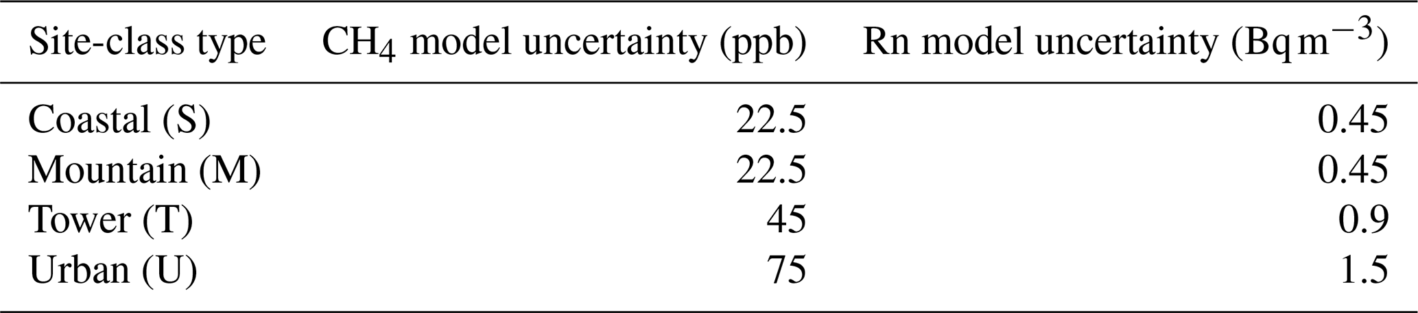
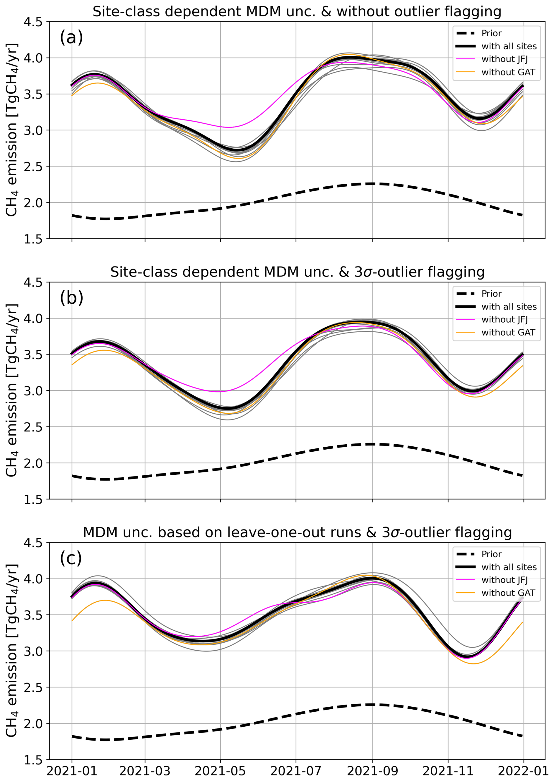
Figure A2 CH₄ flux results for Germany (black, bold lines) from a single-tracer CH₄ inversion based on different setups: (a) site-class dependent MDM uncertainty (magenta curve in Fig. A1) and no outlier flagging (corresponds to the pre-inversion setup), (b) site-class dependent MDM uncertainty (magenta curve in Fig. A1) and 3σ-outlier flagging, and (c) MDM uncertainty based on the pre-inversion leave-one-out runs (orange curve in Fig. A1) and 3σ-outlier flagging. The difference between (a) and (b) is due to the 3σ-outlier flagging, and the difference between (b) and (c) is due to the different MDM uncertainty. The corresponding leave-one-out runs are shown as thin curves.

Appendix B: Evaluation of the dual-tracer approach at independent sites

We evaluate our dual-tracer inversion results at two independent sites in north-western Germany, Steinkimmen (STE) and Jülich (JUE), where both CH₄ and Rn observations are available. These sites were not included in the inversion due to substantial data gaps, particularly in the Rn measurements during 2021. The prior CH₄-Rn MDM correlation coefficients at these sites are r=0.37 (for STE) and r=0.40 (for JUE), which fall within the range observed at the sites used in the inversion but are on the lower end of that range. This suggests that, also at these sites, a part of the CH₄ MDM variability can be attributed to common transport model deficits.

In the CH₄-only inversion, the CH₄-Rn MDM correlation coefficients are reduced, resulting in r=0.21 and r=0.39 at STE and JUE, respectively (see Fig. B1). This is accompanied by a substantial 67 % reduction of the mean (prior) CH₄ MDM at both sites (see Fig. B2a). In contrast, the posterior fluxes from the dual-tracer inversion exhibit higher CH₄-Rn MDM correlation coefficients (r=0.31 for STE and r=0.45 for JUE), leading to a 3 %–7 % higher mean posterior CH₄ MDM compared to the CH₄-only inversion. Under the extreme scenario of assuming a Rn prior flux uncertainty of 5 %, the dual-tracer inversion produces even higher CH₄-Rn MDM correlation coefficients (r=0.35 and r=0.51), attempting to achieve the set correlation of r=0.6, which was assumed in the MDM error covariance matrix. As a result, the prior CH₄ MDM is less reduced, and the fluxes are less adjusted. We also evaluated the performance of the different inversion approaches during situations of low prior Rn MDM (see Fig. B2b, for a prior Rn MDM below ± 0.2 Bq m⁻³). We observe a similar pattern: the dual-tracer yields a slightly higher mean posterior CH₄ MDM than the CH₄-only inversion.

Overall, when the transport model contains systematic biases, the dual-tracer inversion is expected to yield a slightly higher mean CH₄ MDM than the CH₄-only inversion, and thus worse predictive skills. This is because the dual-tracer approach accounts for the fact that part of the CH₄ MDM may arise from transport model errors rather than biases in the prior fluxes, thereby leading to less flux adjustments.

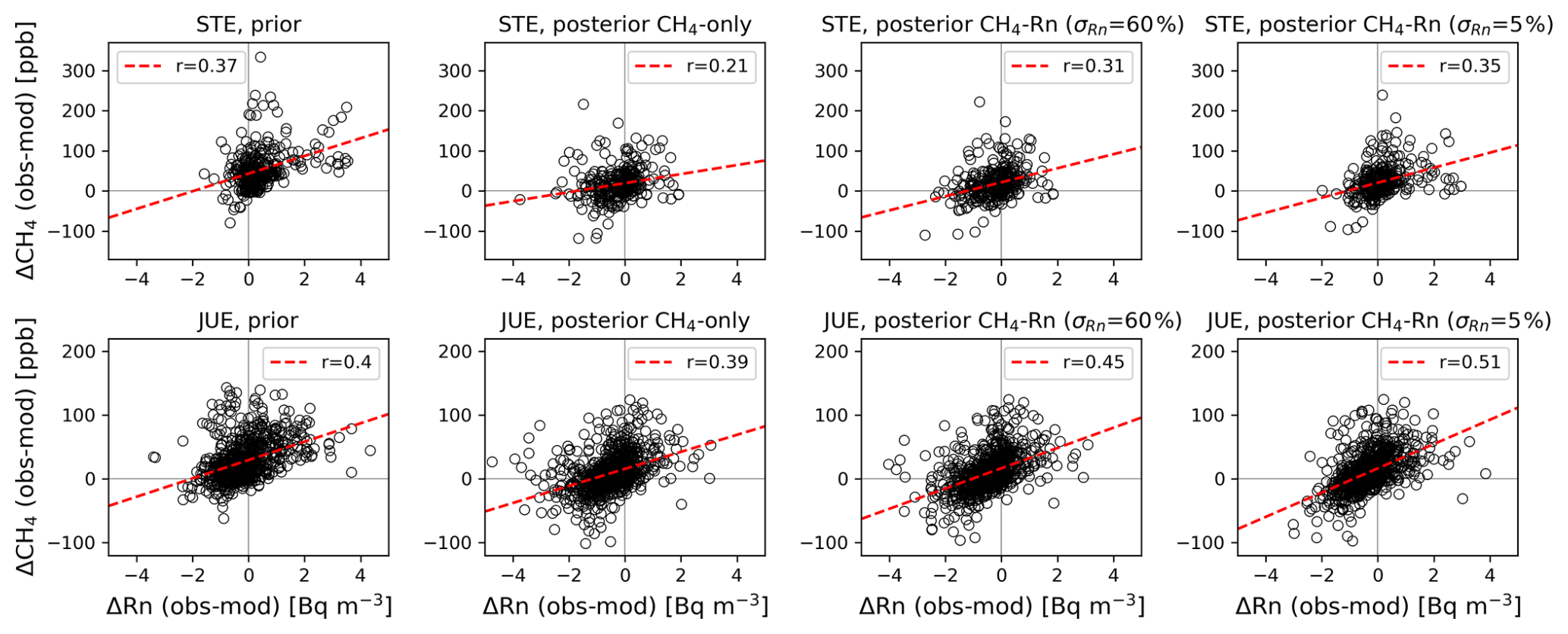
Figure B1 Correlation between CH₄ and Rn MDM at Steinkimmen (top panels) and Jülich (bottom panels) in 2021 for the prior fluxes, the posterior fluxes from the CH₄-only inversion, as well as the posterior fluxes from the dual-tracer inversion for a Rn prior flux uncertainty of 60 % and 5 %, respectively. The CH₄ and Rn observations for STE and JUE are taken from Fischer et al. (2024) and ICOS RI et al. (2024), respectively.

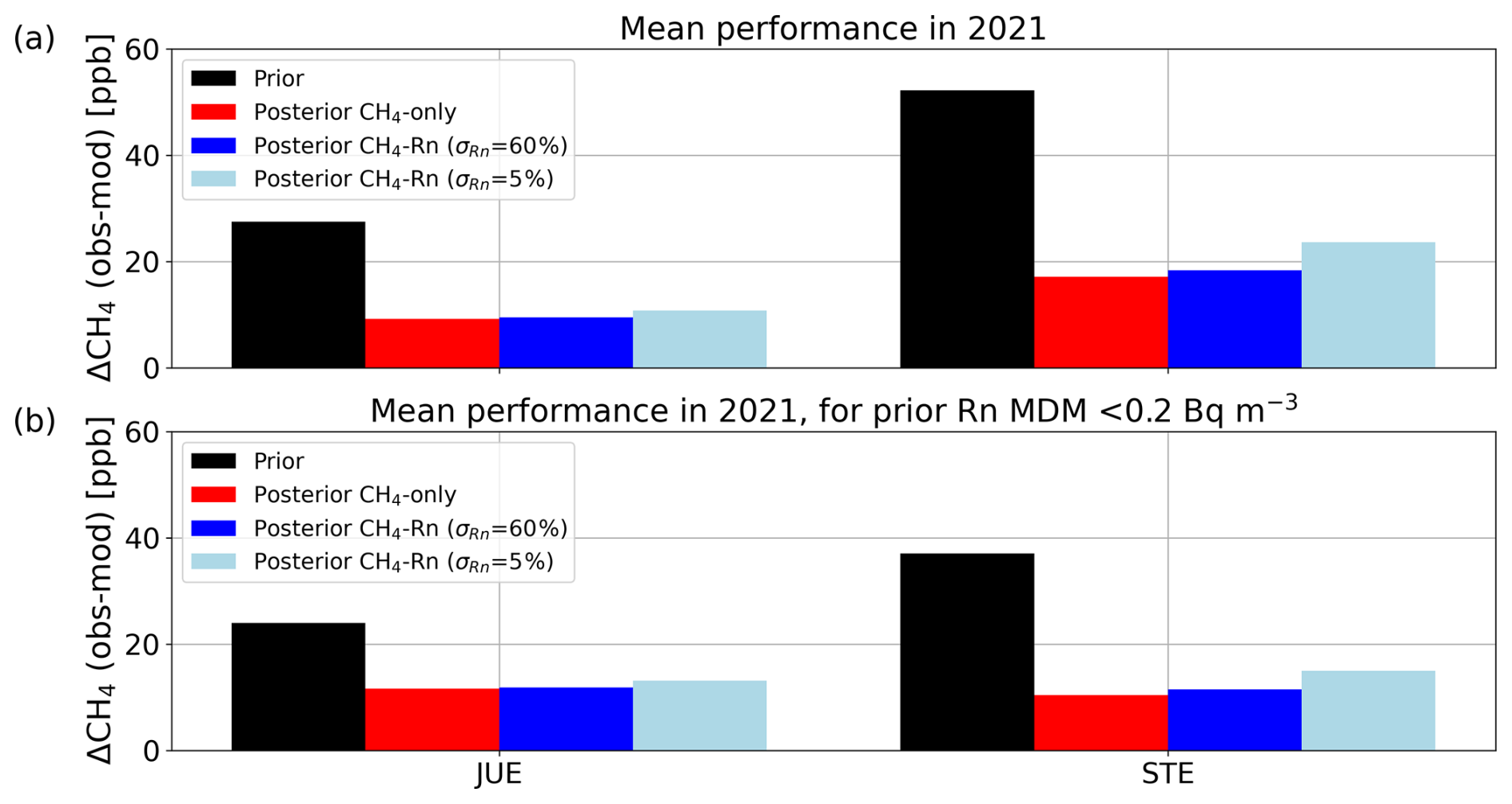
Figure B2 (a) Mean CH₄ MDM at Steinkimmen and Jülich in 2021 for the prior fluxes, the posterior fluxes from the CH₄-only inversion, as well as the posterior fluxes from the dual-tracer inversion for a Rn prior flux uncertainty of 60 % and 5 %, respectively. (b) Same as (a) but restricted to situations where the absolute prior Rn MDM is smaller than 0.2 Bq m⁻³.