On spatial scales of local aerosol production in boreal ecosystems

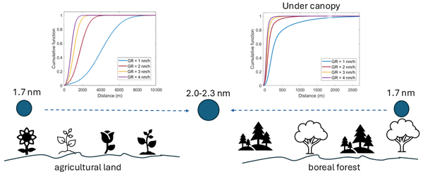
Quantification of the climate impact of land use is important for the development of effective climate change mitigation and adaptation practices. Ecosystems emit compounds that participate in the formation and growth of aerosol particles. Particles of few nm size can be produced locally as compared to regional aerosol growth processes at larger sizes, and in boreal environment, higher concentrations of small particles were observed over agricultural lands than over forests. The aim of this study is to provide estimates of spatial scales of an ecosystem needed to produce small particles predominantly from its own emissions. Here, we consider forest and agricultural ecosystems in the boreal region, and distinguish situations in which aerosol production is relatively slow and vertically distributed within the well-mixed convective boundary layer and when it can occur quickly close to the surface. For the latter, we introduce source contribution function of local aerosol production, which is based on the concentration footprint function modified to account for aerosol growth. We quantify the contributing area for neutral stratification and a typical wind speed. For below-canopy air layer in the forest at 0.5–4 m height from the surface, the relevant distance is at 100–500 m, depending on the growth rate and the initial size distribution. Under the same conditions in the agricultural field, the contribution of the nearby 100–500 m is up to 30 % while the total contributing area is at 0.9–5.5 km. To improve estimates, more research is needed on the dynamics of small aerosol, including contributions of chemical compounds to aerosol growth and the impact of meteorological conditions.

1 Introduction

Land use practices have a profound climate impact (Pielke et al., 2002; Kalnay and Cai, 2003; King et al., 2024). There is a large variability between the climate impacts of ecosystems with different types of vegetation (e.g. comparing forest to rangeland or agricultural land), natural and managed ecosystems (IPCC, 2019). Besides a rather obvious difference in carbon uptake and storage, there are biophysical effects that have to be considered, including the albedo effect on radiation (Betts, 2000; Hasler et al., 2024; Peräkylä et al., 2025), which itself is part of the land use effect on a surface energy balance (Dingman, 2015; Lee et al., 2011; Rinne et al., 2025). Surface conditions directly affect turbulent fluxes relevant for evapotranspiration and development of boundary layer (Stull, 2012), tightly linked to formation and dynamics of boundary layer clouds (Pennypacker and Wood, 2023; Luo et al., 2024).

Furthermore, ecosystems emit volatile organic compounds, which are then oxidized in the atmosphere, contributing to the formation and growth of atmospheric aerosol particles (Tunved et al., 2006; Hallquist et al., 2009; Riipinen et al., 2012; Peräkylä et al., 2014; Huang et al., 2024) and ultimately cloud condensation nuclei (e.g. Petäjä et al., 2022). Aerosol particles associated with emission of volatile organic compounds from boreal ecosystems have been shown to influence the radiative balance of the atmosphere via both aerosol-radiation and aerosol-cloud interactions (Yli-Juuti et al., 2021; Petäjä et al., 2022; Räty et al., 2023; Ezhova et al., 2025).

The formation and growth of aerosol particles in the atmosphere can be briefly described as follows. In the sub-2 nm range, atmospheric molecules form clusters. Atmospheric clustering is a continuous process, so there is always a distribution of aerosol particles in sub-2 nm range. However, growth to larger sizes occurs only occasionally and first as “activation” of particles from approximately 1.7 nm by condensing vapours, which in the boreal environment include highly oxygenated organic molecules (Kulmala et al., 2013; Ehn et al., 2014). At the same time, growing particles are also lost to pre-existing aerosol population, condensation sink. Previous studies show that survival through the 3–5 nm size range is associated with further growth to larger sizes (Aliaga et al., 2023; Garmash et al., 2024; Lampilahti et al., 2025). After approximately 50 nm, the particles can be considered to reach a climatically relevant size, meaning that they can serve as cloud condensation nuclei.

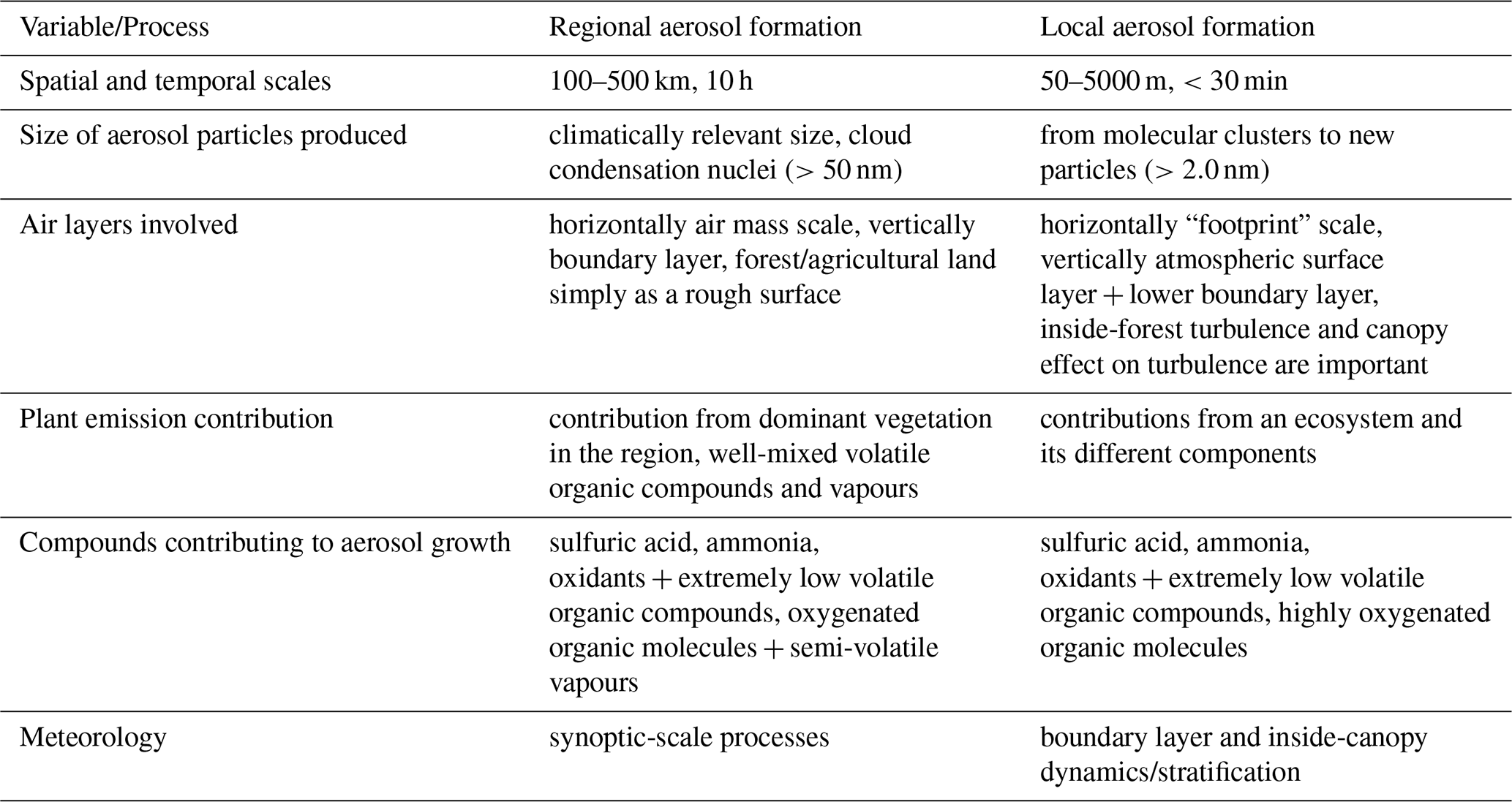
The influence of volatile organic compounds on an aerosol population has previously been considered mainly as a regional phenomenon, with the vapours supporting particle formation and growth towards climatically relevant sizes on large spatial scales (∼100 km) within air masses (Tunved et al., 2006; Paasonen et al., 2013; Petäjä et al., 2022; Räty et al., 2023). However, a recent concept suggests ecosystems as a relatively local source (∼1 km) of nm-size particles or a subrange of intermediate ions (2–2.3 nm) as a proxy for such particles (Kulmala et al., 2024; Tuovinen et al., 2024; Ke et al., 2025). The difference between local and regional aerosol formation is summarized in Table 1.

Table 1 The difference between local and regional aerosol formation.

The concentration of ions in the 2–2.3 nm range demonstrates a reasonable correlation (R=0.61) with the concentration of particles of 3–6 nm (Kulmala et al., 2024; Tuovinen et al., 2026), and to further support this, we show correlations between concentrations of 2–2.3 nm ions and aerosol particles of 2.5–5 nm in Appendix A, Fig. A1, at four sites including forests and agricultural land. As outlined above, survival and growth of aerosol particles depend on the strength of sources of condensable vapours and sinks for vapours and aerosol particles, which change seasonally but also differ on a day-by-day scale. Moderate correlations are therefore expected. Number concentrations of aerosol particles of 2.5–5 nm diameter were linked to regional new particle formation events (Aliaga et al., 2023; Lampilahti et al., 2025). Note also that the growth of ions at the smallest sizes was linked to the further growth of aerosol particles (Kulmala et al., 2004). The potential for 2–2.3 nm ion formation has been assessed for a few sites representing different land use, with the higher number concentrations of ions observed over agricultural ecosystems (Kulmala et al., 2024; Ke et al., 2025).

However, the question about the spatial scale of an ecosystem influencing the growth of smallest particles remains open. Using observations in boreal forest, Kulmala et al. (2013) showed that while the concentration of sulfuric acid vapor is sufficiently high for the smallest particles to grow from 1.2 nm to approximately 1.6–1.7 nm in diameter, further growth cannot be explained by sulfuric acid only, and organic vapours should come into play. The vapours needed to grow the smallest particles should be extremely low volatile, and a recently discovered group of compounds, highly oxygenated organic compounds can possibly account for a large fraction of these vapours (Ehn et al., 2014; Bianchi et al., 2019). These organic vapours are quickly removed from the atmosphere via condensation on aerosol surfaces (Bianchi et al., 2019). As a result, the time scale between the formation of the condensable vapours and their contribution to the growth of the smallest particles is presumably short, potentially making it a relatively local process. However, the condensable vapours are formed as a result of oxidation of volatile organic compounds emitted by an ecosystem, during a finite time, with an impact on the locality. The aims of the current study are:

1. To outline processes contributing to formation of small ions and their growth to 2–2.3 nm, and potential differences depending on the type of ecosystem (forest vs agricultural systems) and discuss conceptual approaches to spatial scale estimation;

2. To quantify horizontal spatial scales corresponding to the growth of ions from 1.7 to 2 nm size linked to an ecosystem via emissions of volatile organic compounds for a simple case of neutral stratification. The aim is to estimate when ion concentration measurements can be interpreted as a contribution of a certain ecosystem, agricultural or forest.

We hypothesize that the spatial scale will depend on the ecosystem functioning (e.g. strength of emissions and emitted compounds), on the physical parameters of the ecosystem (e.g. surface roughness), and on where the measurements are being performed (i.e. the measurement height). Meteorological conditions, such as atmospheric stability and wind speed (and direction, in case of inhomogeneous land cover) will also be important. When interpreting measurements of gas fluxes or concentrations in the surface layer, the concept of footprint area is used, which quantifies the spatial extent of an ecosystem contributing to a measured flux or concentration and is influenced by the same variables (e.g. Vesala et al., 2008). There is thus a certain similarity between greenhouse gases and small ions, both being tightly linked to ecosystems and having climate impacts, but footprint areas of greenhouse gases are not necessarily the same as spatial scales of ion production associated with the same ecosystem.

As difference in 2.0–2.3 nm ions concentrations were observed between measurements done over different ecosystems (Ke et al., 2025), we focus on the horizontal scales affecting ion concentrations. In this paper, we introduce for the first time the source contribution function of local aerosol production and calculate it for two contrasting ecosystems, representing a typical boreal forest and a typical agricultural field. We use a Lagrangian stochastic particle dispersion model (e.g. Vesala et al., 2008), which is suitable for footprint calculations but was not used in aerosol studies before, and modify the outcome to account for aerosol dynamics at the smallest sizes. We limit the current study to a neutral atmosphere, assuming homogeneous turbulence, the simplest turbulence model.

The source contribution function would allow us to estimate the size of an ecosystem needed for producing new particles at the smallest sizes, and to compare it to the typical footprints of greenhouse gas measurements. Understanding on the spatial scales is needed to provide a basis for further research in comparing particle formation potentials of different ecosystems, to better plan measurements for testing theoretical estimates, and ultimately to open ways for modelling studies to quantify the effects of these particles on regional and global climate.

2 Methods

In this section, we provide the overview of the processes involved into formation and growth of aerosol particles at smallest scales, formulate the concept of the source function of local aerosol formation and briefly describe data sets used in the study.

2.1 Overview of the formation and growth of small particles and associated temporal and spatial scales

The process of small aerosol particles formation and growth (speaking mainly about 1.7–2.3 nm particles) has different time scales, influenced by atmospheric chemistry as well as meteorological conditions (wind, temperature, atmospheric stability). In a typical boreal environment, formation and growth of small particles involve three components (in addition to water): sulfuric acid, a stabilizing base (predominantly ammonia) and biogenic vapours (Kulmala et al., 2013; Ehn et al., 2014; Lehtipalo et al., 2018; Olin et al., 2022; Garmash et al., 2024).

Sulfuric acid (H₂SO₄) is formed on site from sulfur dioxide (SO₂) or dimethylsulfide, both having atmospheric lifetimes between about 0.5 and 2 d and thus being transported over relatively long distances, e.g. tens to hundreds of km (Seinfeld and Pandis, 2016). SO₂ is predominantly an anthropogenic pollutant, while dimethylsulfide is emitted by algae. In the absence of strong nearby sources, especially during the warmer season, the precursors of H₂SO₄ are spatially relatively evenly distributed. The major pathway to form H₂SO₄ is through oxidation of precursors by the OH radical, and therefore H₂SO₄ concentrations are highest during the daytime (sunlight promotes OH formation). In Finland, H₂SO₄ formed by oxidation of oceanic dimethylsulfide was found to contribute to the formation of aerosol particles over a boreal forest (de Jonge et al., 2024).

The sources of ammonia include animal waste, fertilizers, anthropogenic activities and ammonification of humus, and are commonly associated with agriculture (Kumar et al., 2025, and references therein). Recent research suggests that the lifetime of ammonia in the atmosphere is about a day with the global mean 22 h (Luo et al., 2022). Similarly to SO₂, the ammonia concentration gradient is expected to be modest outside the vicinity of strong local sources, e.g. agricultural fields.

Oxidized organic vapour formation involves volatile organic compounds (VOC) and oxidants (i.e. ozone (O₃), hydroxyl radicals (OH), and nitrate radicals (NO₃)). In contrast to SO₂, dimethylsulfide and ammonia contributing to small particle formation, VOC are relatively short-lived. The lifetimes of the VOC abundantly released in a boreal environment varies from minutes for sesquiterpenes to hours for monoterpenes (Peräkylä et al., 2014). Therefore, the distances influenced by local sources are much shorter for the main biogenic VOC compared with either H₂SO₄ precursors or ammonia, ranging a few km in case of longer-lived monoterpenes. Coniferous forests are important sources of monoterpenes and sesquiterpenes (e.g. Hakola et al., 2006; Petersen et al., 2025). Agricultural fields also emit VOC, e.g. isoprene, but the role of isoprene in the formation and growth of small particles considered here is not significant. Some studies suggest that agricultural fields are also sources of sesquiterpenes (Ormeño et al., 2010).

A typical boreal landscape, e.g. in Finland, is a mosaic of agricultural fields, wetlands and especially forests representing patches with scales roughly on the order of 1–10 km, skewed to have a larger fraction of the patches at the lower end of this range. All the three components essential to new particle formation (H₂SO₄, ammonia, organic vapors) are expected to be present all over the boreal landscape, even though their relative abundances and contributions likely differ. One could expect ammonia to be the highest over agricultural fields, while most condensable organics are likely to have the highest concentration in forests. The roles of these two components in aerosol formation are different. Ammonia stabilizes sulfuric acid molecules within clusters (e.g. Lehtipalo et al., 2018), but does not not directly influence the growth of such a cluster, which is determined by the sulfuric acid concentration. Arguably, the early growth of clusters and aerosol particles via H₂SO₄-ammonia (amines) clustering mechanism is more typical for polluted sites where both of these components are abundant (Cai et al., 2024; Garmash et al., 2024), and probably also for agricultural sites. Dada et al. (2023) and Kammer et al. (2023) observed a higher ammonia concentration during new particle formation compared to the times with no particle formation. While some studies in polluted environments such as Beijing report that H₂SO₄ and bases alone would be enough to explain particle growth at 1–3 nm (Cai et al., 2024), chamber experiments modelling boreal environment indicate a different story. Indeed, organics can give a totally separate contribution to the particle growth rate, as their thermodynamics (essentially volatility) is not tied to the presence of H₂SO₄. Heavy organic molecules are able to quickly increase the size of small clusters and particles, but they are not as low-volatile as sulfuric acid and probably contribute to the particle growth only at a bit larger sizes, after 1.8 nm (Kulmala et al., 2013; Lehtipalo et al., 2018).

The process of aerosol formation and growth outlined above is sketched in Fig. 1 for agricultural and forest ecosystems. As highly oxygenated molecules (HOM) and ammonia are significant components of aerosol formation and growth directly linked to the ecosystems, we choose to focus on them and not on sulfur compounds or sulfuric acid that can be assumed to be rather similarly available across ecosystems. In the case of forest, this focus makes it possible to consider the activation step from 1.7 to 2.0 nm with the growth times on the order of minutes. The open question is the time scale of conversion of VOC to HOM. This question can also be formulated as how fast can VOC produce condensable organics with concentrations sufficient to contribute to aerosol growth?

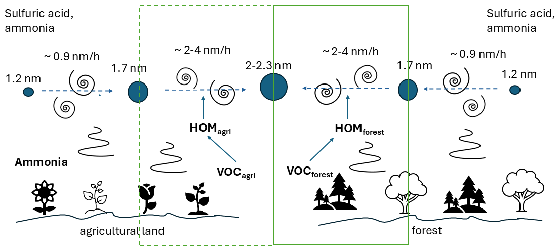
Figure 1 Schematic illustration of the processes contributing to formation and growth of 2.0–2.3 nm ions over agricultural land and forest. Agricultural land emits ammonia and volatile organic compounds (VOC), while forest emits mainly VOC. VOC in agricultural field and in the forest can differ. VOC are oxidized to form highly oxygenated molecules (HOM), i.e. condensable organic vapors. Sulfuric acid is assumed to be formed from sulfur compounds present as background in the atmosphere, ammonia is also present as background. Vortices show turbulence in the atmosphere. 1.2 nm is a representative diameter where sub-2 nm ion distribution typically has a maximum. Aerosol clustering and stabilization (up to 1.7 nm) as well as activation (1.7–2.3 nm) phases in the forest are sketched in accordance with Kulmala et al. (2013), respective growth rates of ∼0.9 and ∼2–4 nm h⁻¹ are estimated from observations. Green rectangular zone focuses on the processes accounted in the calculation of a source contribution function in this study. Note that for forest, the sketched process of aerosol formation and growth can occur both above and under canopy.

In this study, we chose to proceed with species or conditions when the production of HOM from VOC is fast. For example, sesquiterpenes are VOC, emitted by forests, wetlands and other ecosystems, that have a short lifetime and directly satisfy this requirement. However, we argue that longer-lived VOC may also create HOM quickly in non-equilibrium conditions. VOC emission is a non-stationary process influenced by light, temperature and different stress factors (e.g. light stress in spring, drought, or herbivory). In the presence of oxidants, HOM start to form immediately when VOC are released, and their source strength depends on the VOC concentration (see Appendix B). Therefore, strong emissions of VOC, for example, as a result of stress factors, can create concentrations of VOC near the source high enough to quickly produce a sufficient amount of HOM to initiate aerosol growth.

With this in mind, the concept developed in the current study is applicable to situations where VOC quickly form HOM (sesquiterpenes; some fraction of monoterpenes during high emission events), or to emission of ammonia from agricultural fields (ammonia does not need any conversion and condenses as it is). Strong and quick increases in HOM or ammonia concentrations and 2–2.3 nm particles' concentrations could be related to relatively local emissions from the surface. Our data-based estimates show that the total number of the peaks in the 2–2.3 nm concentration time series is larger in forests compared to agricultural fields, and that the number of fast growing peaks comprises about one fourth of all the peaks detected in the forest, and about one third of all the peaks detected in the agricultural fields. Increases in HOM concentrations (at some points, concentration doubles within minutes) were observed at the sites Melpitz and Hyytiälä forest (Jokinen et al., 2014), and increase in HOM and ions concentrations – at Siikaneva (Huang et al., 2024).

Before proceeding with the concept of the source contribution function, we would like to emphasize that other approaches to quantify the scales of local aerosol formation are also possible. One such setup is a well-mixed before-noon boundary layer with a near steady-state VOC (e.g. monoterpenes) concentration. In these conditions, solar radiation provides energy to produce more oxidants, which boosts the production of both sulfuric acid and HOM, contributing to the hour-scale formation of small aerosol particles around noon throughout the boundary layer. In this case, the process occurs in the column of the atmosphere within the boundaries set by wind advection and (turbulent) diffusion from the source. Denoting the lifetime of the prevailing VOC species τ, we can estimate that the horizontal scale of the VOC concentration field $L_{\mathrm{h}}\approx L_{\mathrm{f}}+u\mathit{\tau }$, where L_f is the forest horizontal scale and the second term is due to atmospheric advection of VOC with wind speed u. The vertical scale of the VOC concentration field can be estimated as $L_{\mathrm{v}}\approx \sqrt{\mathit{\kappa }\mathit{\tau }}$, representing turbulent diffusion from the vegetated source surface with diffusivity coefficient κ. Assuming that sulfur compounds and ammonia are available, these scales could be used to estimate the area around the forest, over which VOC from the given forest are abundant and aerosol particles can be formed. Note that in the evening or night when decoupling settles or stable stratification is formed, turbulent mixing is limited, so that after the time on the order of the VOC lifetime, the vertical extent of the layer where aerosol can be formed significantly decreases. With this in mind, we do not claim that aerosol formation at small scales always occurs near the surface but rather outline specific situations, when this can be the case.

Based on the above overview, the “footprint-based” approach is likely to be suitable when VOC emissions and increased concentration govern the formation of HOM needed to initiate aerosol formation and growth, whereas the “boundary-layer” approach is suitable when HOM formation is determined by the increased oxidants concentration. The difference is that oxidants are formed in the column whereas VOCs are released from the surface.

2.2 Concept of the source contribution function of local aerosol production

Within Lagrangian approach to air flow, the observer follows the trajectories of air parcels. These parcels are defined, in accordance with the continuity of the medium, to be small enough to consider different dynamic processes in the atmosphere (e.g. turbulent vortices at small scales), and at the same time large enough to contain many molecules, i.e. large compared to the mean free path of air molecules. We assume that transport of scalar due to diffusion is low compared to that due to advection, so air parcels contain all the same scalar compounds when moving along their trajectories. This is a typical assumption when Lagrangian theory is applied to quantify scalar characteristics of the flow (e.g. Raupach, 1987; Wilson and Sawford, 1996).

In stochastic Lagrangian transport models, concentration of a scalar is defined by averaging contributions of all the air parcels arriving at the measurement point during the measurement time. When footprint for the uniform surface sources is calculated, it is assumed that parcels originated from the surface have the same amount of scalar within them, whereas the air parcels that were not in contact with the surface do not contain this scalar. The concentration footprint function can be calculated as a sum of the contributions from the parcels originating closer or further from the measurement point, which is analogous to them leaving the surface at different time moments. Essentially, it quantifies the area (or typically the upwind distance) from which the scalar-containing parcels arriving to the measurement point were released (e.g. Markkanen et al., 2003). Contribution from sources at different distances depends on horizontal and vertical turbulent transport from the surface sources to the observation level (Fig. 2). Emissions very close to the measurement mast fly off the measurement point as they do not ascend upright. Trajectories originated from far locations at the surface have a small probability to end up at the measurement point; hence a smaller contribution associated with larger traveling times and longer distances. We emphasize here that the time associated with the travel of different parcels from the surface to the measurement point is implicitly included in the footprint concept, even though the footprint function itself is not time dependent.

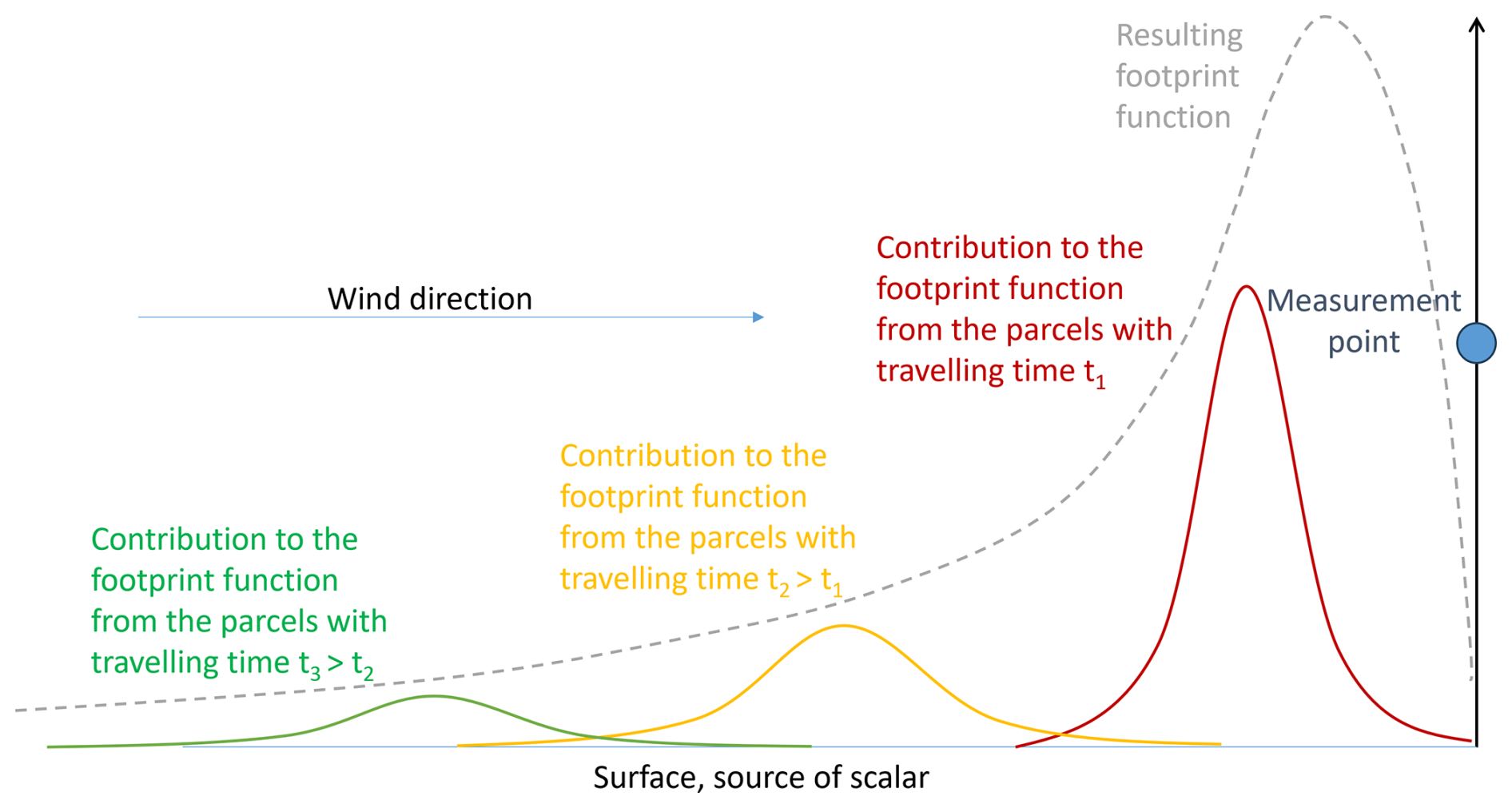
Figure 2 Illustration of the upwind contributions to the footprint function for the air parcels travelling during different times from the moment of emission to measurement. The resulting footprint function is the superposition of all contributions with travelling times $t_{\mathrm{1}}<t_{\mathrm{2}}<t_{\mathrm{3}}$.

The stochastic Lagrangian transport models have also been used to study the transport and footprint functions of non-inert trace gases by implementing a simple first order decay to the tracer concentration in each air parcel (Strong et al., 2004; Rinne et al., 2007, 2012). Our concept of the source contribution function of local aerosol production is related to the concentration footprint for non-inert trace gases as we consider also the time scales of aerosol dynamics. As aerosol formation and growth at small scales is currently better studied for the forest sites, we take Kulmala et al. (2013) concept as a basis (see green area in Fig. 1). Below we list our main premises:

1. organic vapours are essential for the growth of small particles from about 1.6–1.7 nm diameter to 2 nm. The concentration of sub-2 nm cluster ions to be activated by organics is stable within each air parcel;

2. organic vapours needed for the growth of these very small particles should have extremely low volatility and condense quickly. We assume that the tree canopy and understory surface vegetation or soil are sources of volatile organic compounds (VOC) that are oxidized in the atmosphere to rapidly form condensable vapours. As discussed in Sect. 2.1, this assumption can be met if a surface is a strong source of VOC with lifetime of hours (meaning high VOC concentration) or if the lifetime of emitted VOC is short, as for sesquiterpenes.

To summarize, vegetation surfaces are sources of organic vapours that are lost to formation and growth of small aerosol particles within separate air parcels when travelling in the turbulent atmosphere from the source surfaces to the measurement point. The source contribution area of local aerosol production is therefore based on the formulation for the concentration footprint of gases with one important difference: we are interested not in all air parcels that are arriving at the measurements site from the surface but only in those that could contain aerosol particles grown to the size 2.0–2.3 nm during the transport time. This means an additional time-related constraint that can be introduced using sub-2 nm aerosol distribution and the growth rates of the particles. That said, we do not consider separate organic vapours but assume that they provide a certain average constant growth for aerosol particles. This approach is justified for estimates because the link between growth rates and concentrations of highly oxygenated molecules is still a subject of research. Otherwise, we would have to deal with lots of different components with different lifetimes (Peräkylä et al., 2014) and also have to know at which step each of these components contributes to aerosol growth.

We combine the contributions to the concentration footprint function associated with parcels travelling from distance x within time t to the observation point, f(x,t) (see examples in Figs. 2 and 3a), and sub-2 nm aerosol distributions $\mathrm{d}N\left(d\right)/\mathrm{d}\log \left(d\right)$ (see example in Fig. 3b) to calculate source contribution of the local aerosol production. Since we are only interested in the shape of the aerosol distribution as it provides the weights for the footprint contributions, we approximate number-size ion distributions with a Gaussian function N(d,σ), where d is the mean diameter, and σ is the standard deviation. The source contribution function for the production of 2–2.3 nm particles can then be calculated as:

$$\begin{array}{}\text{(1)}& {\displaystyle }{\displaystyle }{f}_w\left(x\right)={\displaystyle \frac{{\int }_{\mathrm{0}}^{T}f(x,t)N(D-\text{GR}t,\mathit{\sigma })\mathrm{d}t}{{\int }_{\mathrm{0}}^{T}N(D-\text{GR}t,\mathit{\sigma })\mathrm{d}t}}.\end{array}$$

where N(d,σ) is the initial distribution of aerosol particles that is assumed to be Gaussian, D=2 nm is the threshold diameter of 2–2.3 nm interval. Aerosol particles in sub-2 nm range are assumed to grow with the same constant rate, GR. This formula can be interpreted as follows: only a certain portion of aerosol distribution can reach 2 nm size during the travel time of an air parcel to the measurement point, therefore, contributions to the footprint function associated with different travel times should be weighted with these portions.

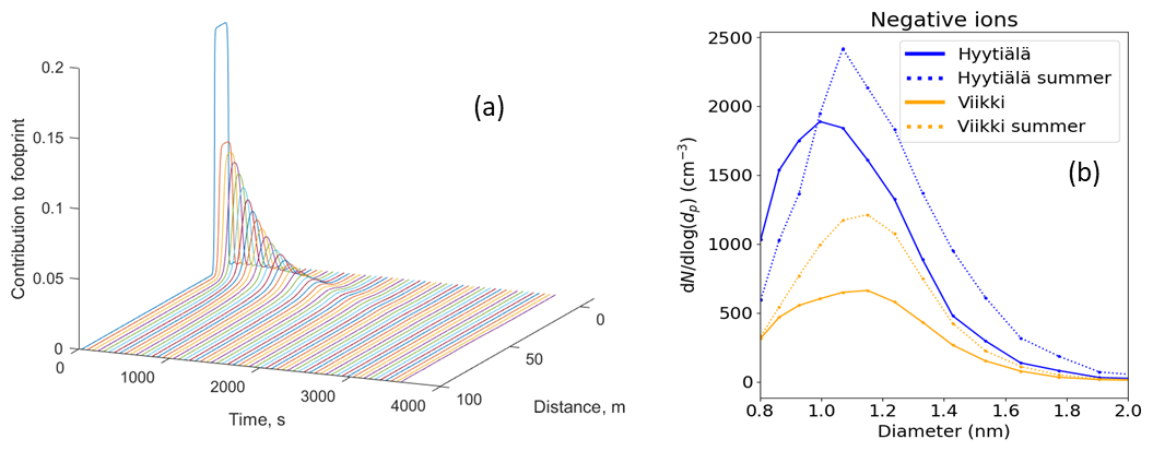
Figure 3 (a) Example of contributions to the inert scalar concentration footprint as a function of the parcel travel time, t, (cf. Fig. 2) and distance, x, to the measurement source f(x,t) calculated for the measurements below forest canopy; (b) median annual and summer sub-2 nm aerosol particle number-size distributions (SMEAR II forest site and SMEAR-Agri agricultural site).

The portion of distribution that can grow to 2 nm during a certain time depends on the initial distribution of sub-2 nm aerosol particles and their growth rates. Previous studies suggest that in the range of diameters between 1.5–2.2 nm the growth rates can vary between 1–4 nm h⁻¹ (Kulmala et al. 2013; same estimates can be obtained from Garmash et al., 2024, Ehn et al., 2014), with 1.5–2 nm h⁻¹ being a more typical value and 4 nm h⁻¹ representing a strong new particle formation event. Since our framework suggests elevated VOC emissions and hence higher concentrations of highly oxygenated molecules, we will make estimates for the range of the larger growth rates, 2–4 nm h⁻¹.

Finally, regarding initial sub-2 nm aerosol distributions used for the calculations: even though Fig. 3b suggests that the aerosol distribution is a Gaussian distribution with the mean value close to 1.15 nm in summer months, not all these particles are able to grow with organic vapours. It is likely that majority of the particles are not growing but correspond to charged molecules and clusters that are always present in the atmosphere as background. The starting diameter when organic vapours are important for growth is about 1.7 nm according to Kulmala et al. (2013).

2.3 Model calculations setup

The calculations of contribution area were performed for two ecosystems, a closed-canopy forest and an agricultural field. Stratification was assumed neutral, and we prescribed a moderate wind speed (friction velocity $u^{*}=\mathrm{0.4}$ m s⁻¹). Calculations were performed for several measurement heights.

The forest height was taken as 20 m, and it was assumed that 25 % of sources were on forest floor and 75 % of sources were proportional to leaf area density (close to the numbers obtained by Petersen et al., 2023). Observation heights included both subcanopy and above canopy levels: 0.5, 1, 2, 4, 21, and 30 m.

For agricultural field calculations, we assumed a surface with roughness z₀=0.05 m (for the typical crops grown in Viikki fields, the vegetation height is between 0–0.7 m, being highest during mid/end of June and again end of July). The source height was assumed to be 1.5×z₀. Observation heights were 0.5, 1, 2, and 4 m.

The Lagrangian dispersion model described in Appendix C was used to calculate the contributions to the inert scalar concentration footprint corresponding to different travel times of the air parcels to the measurement point within 60 min numerical experiments. Note that for the forest calculations, our footprint function is not a footprint function in its traditional sense (i.e. function relating surface sources to the measured concentration), but an aggregate footprint function that weighs the contributions from different levels with the source strength.

In accordance with the premises of the source contribution concept formulated in the previous section, the growing part of sub-2 nm aerosol distribution was assumed to be just a portion of the distributions, considered in Fig. 3b, in their higher end. For simplicity, we assumed it to be Gaussian, with d=1.75 and σ=0.07 nm. Other options and their effect on the resulting contributing area are discussed in Sect. 3.3. The final source contribution function of the local aerosol production was calculated from the convolution of the spatio-temporal contribution function with the aerosol number-size distribution function and normalized with the number-size distribution function, see Eq (1).

2.4 Measurements description

Atmospheric ion size distributions (Fig. 3b) were measured using Neutral cluster and Air Ion Spectrometer (NAIS; Mirme and Mirme, 2013) at the SMEAR II station in Hyytiälä, Finland and at the SMEAR-Agri site in Viikki, Helsinki, Finland. The NAIS is capable of measuring the size distribution of ions with mobility diameters between 0.8–40 nm. The data from Hyytiälä was from 2 February 2010 until 31 December 2024, while the data from Viikki was from 17 June 2022 until 31 December 2024.

3 Results

We quantify the source contribution of the local aerosol formation in forest ecosystem in Sect. 3.1, and in agricultural field in Sect. 3.2. In both cases, we compare the contributing area of aerosol formation to respective inert scalar concentration footprint. The influence of the choice of growing sub-2 nm aerosol distribution on the source contribution function of the local aerosol formation is discussed in Sect. 3.3.

3.1 Footprint area of local aerosol formation in the forest ecosystem

The inert scalar concentration footprint for the forest ecosystem is shown in Fig. 4. The functions corresponding to the below-canopy measurement heights display a high peak near the measurement point. This peak likely originates from the surface emissions, and it is more pronounced compared to above-forest functions because of the dampened subcanopy turbulence. The closer the measurements are to the surface, the higher is the peak, supporting its origin from the surface emissions rather than emissions from the forest canopy.

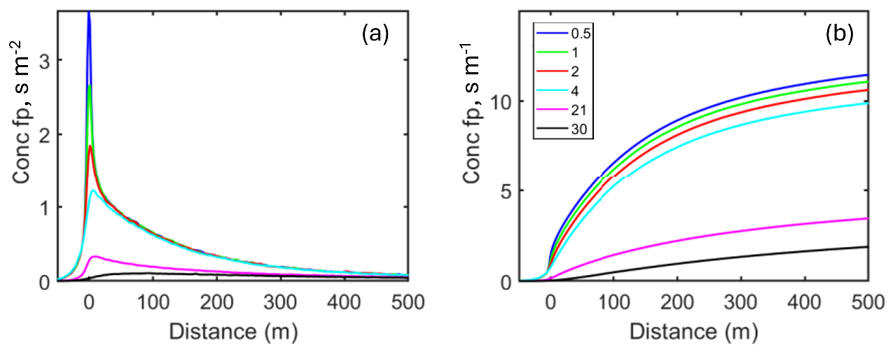
Figure 4 (a) Vapor concentration footprint function and (b) cumulative footprint for the forest ecosystem. Different colors correspond to different measurement heights (see legend, where the heights in [m] are listed). Moving average with the window 3 m is applied to the functions in the left panel. Forest height is 20 m.

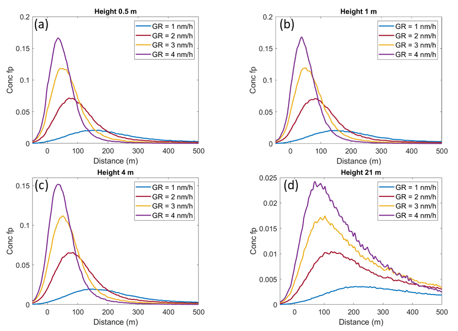
Figure 5 Source contribution areas of the local aerosol production for different measurement heights (see figures' titles) and different aerosol growth rates (different colors and figure legends). Moving average with the window of 3 m is applied to all the functions.

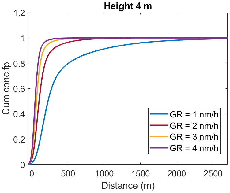
Figure 6 Example of the normalized cumulative source contribution function for the measurement height of 4 m. The 80 % cumulative footprint for aerosol production of 2–2.3 nm diameter particles is the distance where the cumulative function is equal to o.8 (Table 1).

Table 2 The 80 % cumulative distance of local aerosol production of 2–2.3 nm diameter particles in the forest. Due to the stochastic uncertainty of the simulation results, the numbers are rounded to 5 m.

Oppositely, for the measurement heights above the canopy, even at 1 m above canopy top, the peak is much less pronounced due to developed turbulence above the vegetation in neutral stratification: most of the air parcels leaving the surface quickly move up and miss the measurement point but about equally small fraction of them can end up there, resulting in a long tail. At 10 m above the vegetation (i.e. at 30 m measurement height), the peak is very wide and cannot be easily distinguished.

Furthermore, for all the measurement heights, the contributions from close to the measurement point (this peak discussed above) are not significant compared to the tail contributions (see cumulative footprints in Fig. 4b), as the cumulative footprint functions continue to grow at 500 m and after that. This means that the concentration footprint function is delocalized, i.e. the parcels which come to the measurement point could originate from far locations. The cumulative concentration footprint of inert gases, for example, CO₂, does not saturate with distance.

Figure 5 shows the source contribution functions of local aerosol formation for different measurement heights and growth rates of aerosol particles. Note that the peak is now moved further from the very close vicinity of the measurement point towards 50–200 m; the larger the growth rate, the more pronounced the peak is and the closer it is to the measurement point. At the same time, the difference between the functions corresponding to the different measurement heights below the canopy is small. This behaviour of source contribution functions is dependent on the initial distribution of sub-2 nm aerosol particles and footprint contributions for different air parcels travel times. The peak is now defined not only by the largest contribution of f(x,t) to the footprint as in Fig. 4, which of course occurs for short travel times featuring the area in the vicinity of the measurement point, but also by the weighing function. If there are too few aerosol particles close to 2 nm size in the sub-2 nm distribution, it would mean that in the air parcels originating near the measurement point, they do not have time to grow to the 2 nm size, and thus, large contribution from vapours emitted nearby the measurement mast does not appear in the source contribution function of local aerosol production. Instead, the peak corresponds to the parcels originated further from the measurement point, associated with longer travel times. Note that the biggest difference between the vapor concentration footprint functions (peaks in Fig. 4a) under forest canopy resulted from these close contributions. When the aerosol distribution-weighing dampens it, there is in practice almost no difference between the different measurement heights (Fig 5a and c, heights 0.5–4 m). Moreover that only part of the aerosol particles can grow to larger sizes (meaning contribution of initially small particles is also dampened) makes the source contribution functions of the local aerosol production more localized compared to the normal vapor concentration footprint functions, and the cumulative functions saturate with distance (see example for 4 m height in Fig. 6). Thus, we can now normalize the cumulative concentration footprint function with its saturated value to obtain fractional contributions to the footprint, for example, the 80 % cumulative footprint for aerosol production of 2–2.3 nm diameter particles, meaning the distance where the cumulative function reaches 80 % of its saturation value (Table 2).

From Table 2, under the forest canopy, the area contributing 80 % to concentration of 2–2.3 nm aerosol particles is about 100 m for the fastest growth rates of 3 and 4 nm h⁻¹, about 200 m for the growth rate of 2 nm h⁻¹ and 0.5 km for the slowest growth of 1 nm h⁻¹. For the measurements above the forest (1 m above the canopy), all the distances approximately triple.

3.2 Source contribution function of local aerosol production over an agricultural field

In this subsection, we consider source contribution areas of the local aerosol production calculated for the agricultural fields using the same initial aerosol distribution and growth rates as in the previous section.

We again start with the standard inert scalar concentration source contribution functions (Fig. 7). It shows a stronger contribution of the nearby area if the measurement point is located closer to the surface (blue curve at 0.5 m above the surface), whereas the peak is much wider at 4 m height. Also for this ecosystem, the cumulative functions exhibit growth without tendency to saturation still at the furthest points shown in the figure, similar to the functions in Fig. 4.

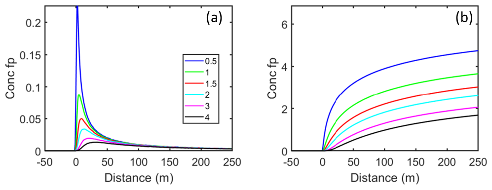
Figure 7 (a) Vapor concentration footprint function and (b) cumulative footprint for the agricultural field. Legend shows measurement heights in [m].

The source contribution function of the local aerosol production for the agricultural field exhibit behaviour qualitatively similar to that of the functions calculated for the forest: peaks become localized further from the measurement site and tails become dampened. However, it is located much further from the measurement point compared to the forest subcanopy simulations, at 0.5–4 km compared to ca 200–500 m (Fig. 8). The cumulative functions reach 80 % of the saturated values within 1–5 km depending on the growth rate (Table 3, two first rows), about tripling the values obtained for the measurement height 1 m above the forest canopy. At 4 m height, the functions are similar to 0.5 m, also quantitatively (Table 3).

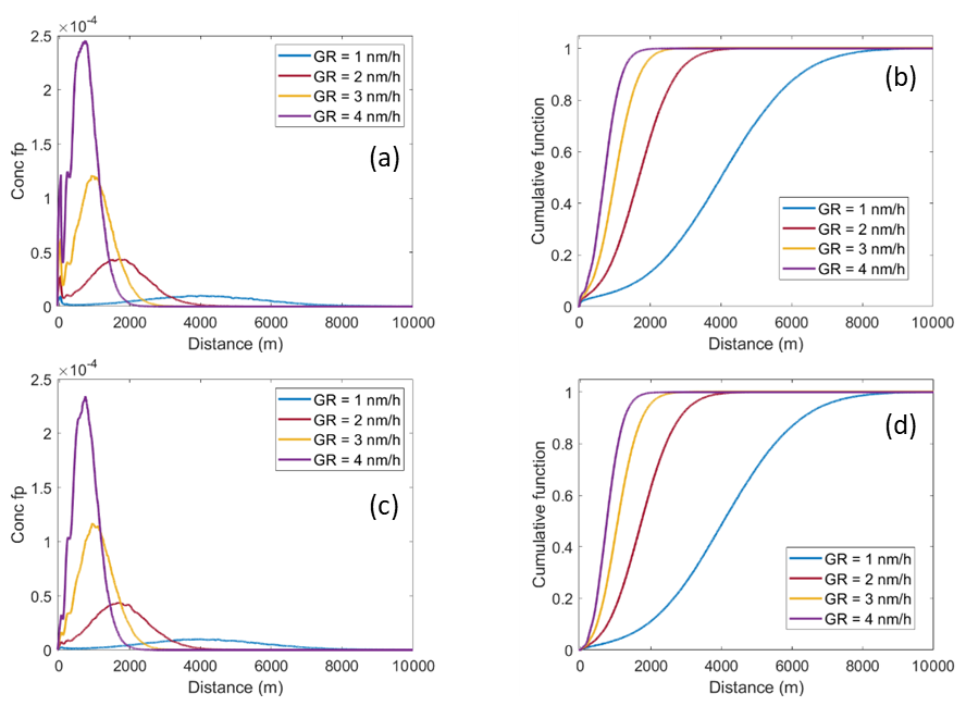
Figure 8 Source contribution functions (b, d – normalized cumulative) at 0.5 m height (a, b) and at 4 m (c, d), agricultural field. Initial aerosol distribution function is the same as for forest calculations (d=1.75 and σ=0.07 nm). Moving average with the window 101 m is applied to the functions in panels (a) and (c).

Table 3 The 80 % cumulative area of local aerosol production of 2–2.3 nm diameter particles in the fields. Case 1 corresponds to the function with d=1.75, σ=0.1 nm, Case 2 to the function with d=1.15 nm, σ=0.25 nm (Sect. 3.3). Due to the stochastic uncertainty of the simulation results, the numbers are rounded to 0.1 km.

3.3 Effect of the initial sub-2 nm aerosol distribution on the source contribution function of local aerosol production

In this subsection, we consider the effect of different initial aerosol distributions on the source contribution functions. We perform analysis for agricultural fields, in which case the source contribution functions show higher sensitivities to changes in different model variables (the peak position can be much further from the measurement point, see Figs. 5 and 8).

In Sects. 3.1 and 3.2, we accounted for the fact that only a portion of the sub-2 nm particles is able to grow due to organic vapours, and modelled it using Gaussian function with diameter 1.75 and σ=0.07 nm (Fig. 8). Here we assess the impact of initial sub-2 nm distribution on the final source contribution area of local aerosol production, changing parameters of the Gaussian function: Case 1) wider initial distribution, so that there are already some particles in the tail at 2 nm size (d=1.75 and σ=0.1 nm); Case 2) the whole initial sub-2 nm distribution can grow due to organic vapours (a wide distribution with σ=0.25 and d=1.15 nm far from the 2 nm threshold). Case 1 is close to the points obtained from the measured distributions (Fig. 9), whereas Case 2 is an unlikely situation and serves to illustrate the effect of d and σ on the source contribution function. In this section, we consider only one measurement height of 0.5 m, as the functions at different heights are similar to each other.

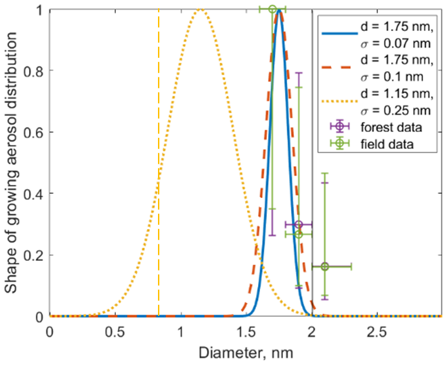
Figure 9 N(d,σ) when only a part of the distribution is allowed to grow (solid and dashed) or when the whole distribution can grow (dotted). Points are obtained from measurements (median, 25th/75th percentiles) in the forest (SMEAR II, 2020–2024) and agricultural field (Viikki, 2023–2024). Vertical dashed line denotes 0.8 nm, an approximal threshold between molecules and small aerosol particles. Strictly speaking, the distribution of sub-2 nm aerosol is not defined below this threshold, so we keep the tail as one option for the calculations in the unlikely case when the distribution grows as a whole.

First, we consider probably the most relevant situation, where a small portion of aerosol particles in the initial distribution is already at 2 nm (see the points obtained from normalized median distributions for the forest and field in Fig. 9). The results are shown in Fig. 10: the main difference to Fig. 8 is a bigger contribution from the nearby area of 100 m. About one third of the cumulative contribution to aerosol concentration is now from this nearby location of about 100 m whereas the 80 % cumulative source contribution is within 0.9–2.0 km depending on the growth rate (excluding the smallest growth rate GR=1 nm h⁻¹).

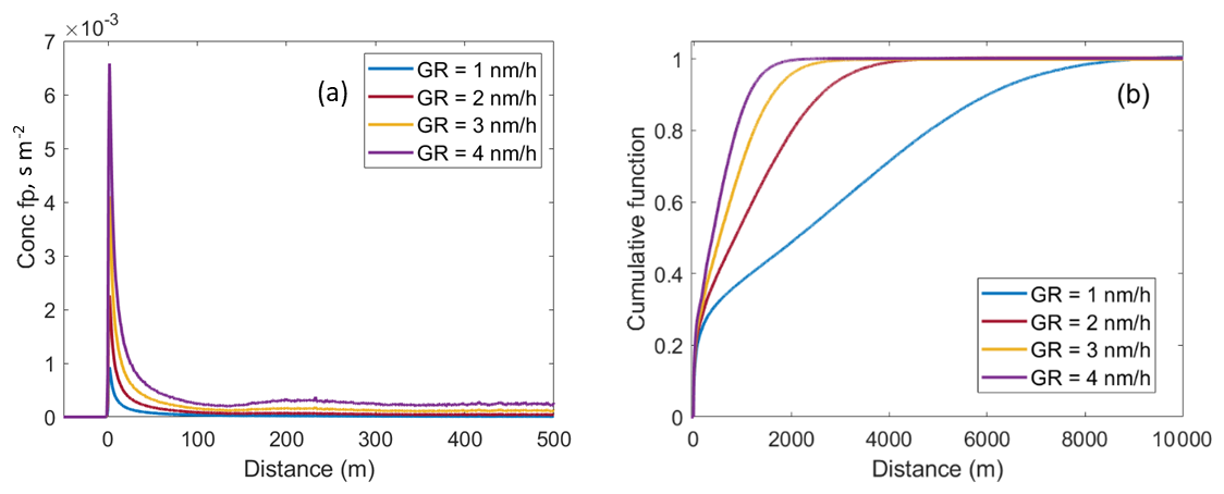
Figure 10 Source contribution functions for the initial sub-2 nm distribution with d=1.75 and σ=0.1 (Case 1, Fig. 9). Measurement height is 0.5 m.

When we use a full median initial distribution which is also located closer to 2 nm threshold, meaning that fraction of the particles can grow relatively quickly, we expect both a high peak in the vicinity of the measurement and longer saturation distances because of the width of the function. The results for the Case 2 are shown in Fig. 11. There is indeed a narrow peak near the measurement site, but also wider peaks at a few km distance, and the saturation occurs much further compared to all the previous cases. The 80 % cumulative functions are at the distances of 6–10 km from the measurement points at GR=3 and 4 nm h⁻¹ so the contributing areas are very large. At GR=1 nm h⁻¹, the cumulative source contribution just starts to grow.

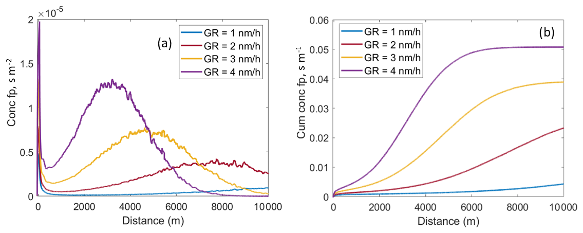
Figure 11 Source contribution functions for the initial sub-2 nm distribution with d=1.15 and σ=0.25 nm (Case 2, Fig. 9). Measurement height is 0.5 m. Moving average with the window 101 m is applied to the functions in the left panels. The cumulative functions are not normalized because functions at the lowest GR do not saturate at 10 km.

In general, the conclusions from the use of different aerosol distributions are as follows. The functions under integral in Eq (1) both have maxima: there is a maximum in aerosol particle distributions and in the functions f(x,t) contributing to the concentration footprint. The resulting source contribution area of the local aerosol formation has a noticeable maximum in the near vicinity of the measurement point if there are particles in aerosol distribution that can grow quickly. If the share of these particles is small as in the narrow distribution (blue curve in Fig. 9), then the near peak is not visible, and there is a dominating peak further from the measurement point due to weighing the tails of f(x,t) by aerosol distribution also having a maximum (Fig. 3). In other words, the source contribution function of the local aerosol production has two peaks with their relative contribution depending on the growing aerosol initial distribution and growth rates.

4 Discussion

Here we made estimates of how large an ecosystem needs to be for us to assign measured concentrations of small aerosol particles to ecosystem's own emissions. Tuovinen et al. (2024) made a simple estimate of the spatial scales of the ecosystem that can influence small aerosol particles during their time of growth by 1 nm in diameter. Their estimates were based on the advective transport and, for the wind speeds and growth rates used here, resulted to scales between 1–15 km. Our results, based on the concept of the footprint and accounting for turbulent transport, suggest that the spatial scale depends strongly on the fraction of the aerosol distribution growing due to the condensation of organic vapours. In addition, for the forest ecosystem, there is clearly a big difference if the measurements are done below or above the canopy, with the implication that below the canopy, the area affecting local aerosol production is localized to within 500 m even for very small growth rates.

Here we assumed that volatile organic compounds (VOC) are converted to low-volatility organic vapours condensing on aerosol particles immediately after their emission. However, oxidation of typical VOC emitted by ecosystems is not indefinitely fast and occurs during finite times depending on the availability of VOC and oxidants (e.g. Peräkylä et al., 2014) with an implication that the source contribution area of small aerosol production can increase. Here we outlined conditions for this process to occur within minutes.

We notice that the main difference in the contribution area between agricultural land and forest appears due to the difference of open area over agricultural land vs. sheltered area below the forest canopy. Above the canopy, the behaviour of forests seems quite similar to agricultural land as expected. Potential differences in aerosol dynamics due to emissions of specific chemical compounds are not taken into account here because of the lack of knowledge on aerosol formation and growth as well on connections between VOC and highly oxygenated molecules over agricultural fields.

The effects of meteorology should be considered further in future studies. An especially striking example is the decoupling in the evenings when temperature quickly drops, which is known to boost ion clustering both in a forest and over the peatland sites (Zha et al., 2018; Huang et al., 2024). The contribution of different components to the particle formation and growth during decoupling is not entirely clear. If there are on-going emissions of VOC from any nearby sources, dilution of these components is inefficient in a shallow stable boundary layer, so they can be converted to vapours and further to aerosol. Note, however, that sources of vapours are not necessarily on the surface, and gravity flows can bring VOC from nearby forests (Huang et al., 2024). Moreover, if in summer, as Stolzenburg et al. (2025) suggest, there are already abundant organic vapours which do not condense, a decrease of temperature can trigger a decrease in the volatility of these vapours, making them to condense more easily. In the latter case, the process will still be local but not directly related to the surface (besides potential landscape influence which can support formation of a decoupled layer).

Finally, especially formation of aerosol in agricultural ecosystems is severely understudied, with basically two research sites up to date (in France and Finland, Dada et al., 2023; Kammer et al., 2023). This opens new research directions: statistics and comparability of aerosol dynamics in forests and agricultural sites, the role of ammonia and other VOC emissions in aerosol formation growth in agricultural fields, and the effect of meteorological conditions. Finally, previous knowledge on importance of forest emissions for aerosol growth on a regional scale offers a perspective on a synergistic role of agricultural fields dominating small aerosol production and forests contributing vapours for further growth of aerosol towards climatically relevant size.

5 Conclusions

The source contribution function of the local aerosol production is introduced to quantify the spatial scales of an ecosystem needed to separate its contribution from the neighbouring ecosystems. Aerosol-related functions are compared to the standard vapor concentration footprint functions. We show that the source contribution areas of local aerosol production are strongly sensitive to the initial sub-2 nm aerosol distribution (or, strictly speaking, the portion of this distribution that can grow to 2 nm sizes due to organic vapours) and growth rates of aerosol particles. If initially the portion of aerosol particles close to 2 nm is small, the contribution of the nearest area is strongly suppressed. However, this is not the case if there are particles close enough to 2 nm that are able to grow quickly.

For the neutral stratification considered here, our results suggest that the source contribution function of local aerosol production is not sensitive to the measurement height (0.5–4 m for agricultural fields), clearly except the case of measurements below and above the forest canopy. This is because the requirement for aerosol growth to 2.0 nm dampens the input of the air parcels from the nearby area. This contribution defines the difference between the traditional concentration footprint functions at different measurement levels, i.e. a stronger input from the nearby area at the lowest measurement levels.

Previous estimates of the spatial scale of local aerosol formation based on mean advective transport, for the same wind speeds and growth rates as we used in this study but not distinguishing between different ecosystems and not accounting for aerosol distribution, landed between 1–15 km (Tuovinen et al., 2024). Ecosystem type, in particular canopy structure, which is important for turbulent transport, and initial sub-2 nm ion distribution, which together with growth rates and wind flow determine contribution of air parcels from a certain distance, are essential for the estimate. Therefore, the numbers obtained here differ from those in above-mentioned study. For subcanopy aerosol formation in the forest, the spatial scale is within 0.5 km even for low aerosol growth rates. Just above the forest canopy, the scale is on the order of 0.5–1.5 km, and it increases to 0.9–5.5 km in open areas with low roughness such as agricultural fields. While the approach used here can be applied to make estimates of source contribution function in various ecosystems, the forest properties in the turbulent transport model correspond to pine-dominated boreal forest with closed canopy typical for Finland, and thus, exact numbers obtained here have a regional rather than global character. All in all, here we made better elaborated but still relatively simple estimates and discussed physical and chemical processes and phenomena potentially to be accounted for in future: e.g. difference in chemical compounds emitted by agricultural lands and forests or local meteorological conditions.

In agricultural fields, we get few km estimates for the scale of the local aerosol formation, which is roughly similar or larger than the inert scalar flux footprint area calculated in previous studies for grassland (Kljun et al., 2002). Note, however, that the source contribution function introduced here for the local aerosol formation is fully different from inert scalar flux footprint function, and is based on the like of the concentration footprint and initial aerosol distribution. Below canopy in the forest, emissions from the canopy and soil are accounted in the source contribution function unlike for the concentration footprint, in which case only underlying surface is the source of scalar.

Thus, for us to be able to separate the aerosol particle production from a specific agricultural system, a fetch of few kilometers is needed. For measurements conducted in forest ecosystems the fetch can be smaller, within 1.5 km or even within 500 m if measurements are done below the canopy. Having in mind different processes influencing local aerosol production provided in this study, we need to quantify better the dynamics of the ions (peaks, their time scales, strength) and link it to atmospheric conditions, including chemistry and meteorology. This is important to recognize when measurements and conclusions about the potential of different ecosystems to produce aerosols are being made, and to understand whether and how different ecosystems are cooling climate via aerosol production.

Appendix A: Correlations between daily peak concentrations of 2.0–2.3 nm negative ions and 2.5–5 nm aerosol particles

We used the data measured with Neutral cluster and Air Ion Spectrometer (NAIS) at fours sites in Finland: SMEAR I station in Värriö (subarctic pine-dominated forest), SMEAR II station in Hyytiälä (pine-dominated forest in southern Finland), as well as SMEAR-Agri site in Viikki, Helsinki (agricultural suburban), and Qvidja in Parainen (agricultural), both in southern Finland. The measurement periods used covered January 2016–September 2024 in Hyytiälä, February 2019–November 2024 in Värriö, June 2022–January 2025 in Viikki, and October 2019–January 2025 in Qvidja.

First, we calculated the peak concentration of 2–2.3 negative ions above its background value for each day from time series with hourly resolution. For each site and day, the hourly 2.0–2.3 nm ion number concentration was denoted as $N_{s,d,h}$, where s is the site, d is the calendar day, and h is the hour of day. The daytime activity window for each day d and site s was selected as the consecutive 7 h window within 08:00–19:00 that had the highest mean concentration:

$${\displaystyle }{\displaystyle }{W}_{s,d}^{\text{day}}=\underset{W\in {\mathrm{W}}^{\text{day}}}{\arg max}{\displaystyle \frac{\mathrm{1}}{\left|W\right|}}\sum _{h\in W}{N}_{s,d,h},$$

where W^day contains all consecutive 7 h windows fully inside 08:00–19:00, and where W∈W^day is a single 7 h window that starts earliest at 08:00, and latest at 13:00 LT. The daytime maximum was then defined as

$${\displaystyle }{\displaystyle }{N}_{s,d}^{\text{max}}=\underset{h\in W_{s,d}^{\text{day}}}{max}{N}_{s,d,h}.$$

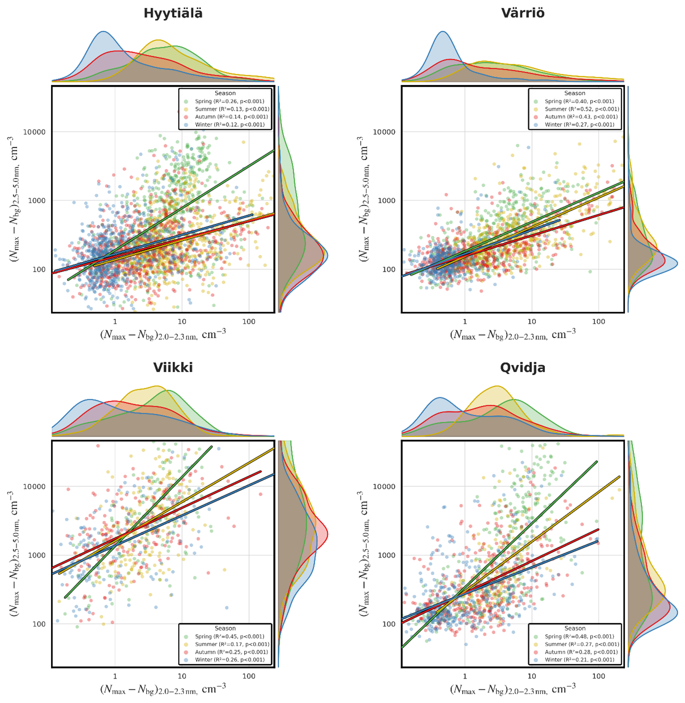
Figure A1 Correlations between the peaks in number concentration relative to their respective background values, daily time scale: x axis 2–2.3 nm ions, y axis 2.5–5 nm aerosol particles. Colorcode is season; lines show correlations for different seasons, R coefficients and p values are reported in the legends. Hyytiälä and Värriö are forest sites, Qvidja and Viikki are agricultural sites.

The background window was defined as the consecutive 5 h window within the same calendar day that had the lowest mean concentration, excluding hours that overlapped with the selected daytime activity window or with nighttime activity hours belonging to that calendar day:

$${\displaystyle }{\displaystyle }{W}_{s,d}^{\text{bg}}=\underset{W\in W^{\text{bg}}}{\arg min}{\displaystyle \frac{\mathrm{1}}{\left|W\right|}}\sum _{h\in W}{N}_{s,d,h}.$$

The background concentration was calculated as the median concentration within this selected background window:

$${\displaystyle }{\displaystyle }{N}_{s,d}^{\text{bg}}={\text{median}}_{h\in W_{s,d}^{\text{bg}}}\left(N_{s,d,h}\right).$$

Finally, the daily peak-minus-background concentration of 2–2.3 nm negative ions was calculated as

$${\displaystyle }{\displaystyle }\mathrm{\Delta }{N}_{s,d}^{\text{day}}={\left(N_{s,d}^{\text{max}}-N_{s,d}^{\text{bg}}\right)}_{\text{2.0–2.3}\mathrm{nm}}.$$

We then calculated correlations between the daily peak concentrations of ions above background values with similarly defined concentrations of larger total aerosol particles in the range 2.5–5.0 nm (Fig. A1). This latter metrics, (N^max−N^bg)_{2.5–5.0 nm}, was previously used in nanoparticle ranking studies in Finnish and Siberian taiga. Here we use previously unpublished data also from other Finnish sites.

Figure A1 shows statistically significant positive correlations for all sites. One can notice a difference between the seasons: especially spring values of (N^max−N^bg)_{2.5–5.0 nm} (y axis) are typically higher and spring correlations are in general stronger; spring is the season when new particle formation is typically the most frequent and intense. The only site where green lines are close to others is the subarctic forest, where thermal spring occurs often within calendar summer. Seasonal correlations are weaker in Hyytiälä compared to other sites, most likely due to the longest data set. One can clearly see two clouds of points in the Hyytiälä panel along two lines, where one is more associated with spring, and another with remaining seasons, but it is obvious that simple seasonal separation is not optimal. A more detailed investigation requires consideration of sources and sinks, as well as meteorological conditions, and is beyond the scope of this study. All in all, while correlations depend on many factors, they are clearly visible, and associations of small ions' concentration with that of larger aerosol particles are statistically significant at the 0.001 level and positive for all the sites and in all the seasons.

Appendix B: Concentration of oxidized organics at short times after emission

Here we derive a formula for the concentration of oxidized organics [ELVOC] in the limit t→0. Following Ehn et al. (2014), consider dynamics equation modified to account for the presence of different oxidants:

$$\begin{array}{ll}{\displaystyle \frac{\mathrm{d}\left[\text{ELVOC}\right]}{\mathrm{d}t}}& {\displaystyle }=\text{OR}\left[\text{VOC}\right]-\text{CS}\left[\text{ELVOC}\right]\\ \text{(B1)}& {\displaystyle }& {\displaystyle }=Q-\text{CS}\left[\text{ELVOC}\right],\end{array}$$

OR – oxidation rate accounting for the presence of all different oxidants (depends on the oxidants' concentrations and reaction rates only) with time scales of min-hour (there can be some coefficient, similar to γ in Ehn et al. 2014, decreasing the effectiveness of oxidation), [VOC] is a concentration of any VOC compound, for example, monoterpenes, Q is the source of extremely low volatile organic vapours (ELVOC) and CS is a condensation sink.

Solution of Eq. (B1) is

$$\begin{array}{}\text{(B2)}& {\displaystyle }{\displaystyle }\left[\text{ELVOC}\right]={\displaystyle \frac{Q}{\text{CS}}}\left(\mathrm{1}-\text{exp}(-\text{CS}\cdot t)\right).\end{array}$$

This means that the time scale of ELVOC relaxation to its steady state is solely defined by the condensation sink. The higher concentration of VOC leads to higher steady-state concentration of ELVOC, while lower oxidation rates (lower oxidants' concentration) counteracts it.

Now consider the solution (B2) at very short times in the limit t→0, the exponent can be expanded to the series: $\text{exp}(-\text{CS}\cdot t)\approx \mathrm{1}-\text{CS}\cdot t$. Then

$$\begin{array}{ll}{\displaystyle }\left[\text{ELVOC}\right]& {\displaystyle }\approx {\displaystyle \frac{Q}{\text{CS}}}\left(\mathrm{1}-\mathrm{1}+\text{CS}\cdot t\right)\\ \text{(B3)}& {\displaystyle }& {\displaystyle }=Qt=\text{OR}\left[\text{VOC}\right]t={\displaystyle \frac{\left[\text{VOC}\right]}{\mathit{\tau }}}t.\end{array}$$

so at short times, the concentration of ELVOC is inversely proportional to the lifetime of VOC components and directly proportional to the concentration of VOC.

Appendix C: Lagrangian stochastic trajectory simulation within and above canopy

For Lagrangian stochastic trajectory simulations the model satisfying the well-mixed condition was used, choosing the Gaussian distribution of velocity fluctuations (Thomson, 1987) for neutral Atmospheric Boundary Layer (ABL) conditions considered in this study. We applied forward trajectory simulation method. We note that for our turbulence model, it does not matter which approach is used, backward or forward simulations. In case of horizontally homogeneous turbulence assumed in this study, the most straightforward approach is to use forward simulation. The concentration due to sources located within canopy was estimated from trajectory statistics crossing the observation level (e.g. Markkanen et al., 2003).

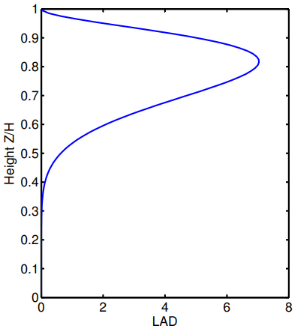
Figure C1 Profile of leaf area density (LAD) used in the Lagrangian model forest simulations.

Turbulence statistics inside canopy were derived using the analytical canopy turbulence 2nd order closure model by Massman and Weil (1999). Above canopy, the Atmospheric Surface Layer profiles were used (e.g. Kaimal and Finnigan, 1994), which were matched with the ABL turbulence profiles based on Rotach et al. (1996) and de Haan and Rotach (1998). For simplicity, ABL height was fixed at 1000 m over agricultural field characterized by surface roughness 0.05 m and at 2000 m over forest canopy with average tree height of 20 m. In the simulations, we assumed homogeneous surface cover, either forest or agricultural land, so the effect of small patches is not considered. The displacement height and roughness length characteristics for the pine forest were derived from the model and were equal to 16.7 and 1.4 m, respectively. We simulated leaf area index of 2.5 corresponding to pine or spruce, dominant species in Hyytiälä (Launiainen et al., 2022), with leaf area density (LAD) profile shown in Fig. C1). Absorption of air parcels at the top of ABL was assumed.