An observational perspective on precipitation efficiency of mesoscale convective systems over the Asian Monsoon Region

This study investigates the precipitation efficiency (ε) of tropical mesoscale convective systems (MCSs) using satellite-based precipitation rates ($\dot{P}$) and reanalysis cloud, ice, and liquid water paths (CWP, IWP, LWP). We define ε as the ratio of $\dot{P}$ to CWP, following Li et al. (2022), and phase-partition it using IWP and LWP. We calculate these metrics for a total of 1321 MCSs tracked by the Python FLEXible Object TRacKeR (PyFLEXTRKR) algorithm and focus on southern Asia during monsoon season, given its frequent MCS occurrence. We first look at spatial distributions, analyzing longitudinal and latitudinal trends in MCS versus non-MCS ε. MCS ε values are 50 % higher than ε from non-MCS convection on average and increase from north to sorth and from west to east along monsoonal moisture gradients. Decompositions of ε across different regions of the MCSs indicate that the highest ε consistently occurs within the core, followed by the cold and then warm anvils. Scaling ε by MCS area shows that all ε metrics increase with area up to an MCS effective diameter of 160 km. This trend is consistent with enhanced ice growth associated with deeper clouds and stronger convective organization in larger MCSs, before ε decreases again in the largest systems where cloud ice growth has reached its maximum. In contrast, all ε metrics increase monotonically with MCS depth, indicating that deeper systems convert cloud condensate into surface precipitation more efficiently without the non-monotonicity observed in the ε-area scalings. Finally, ε increases rapidly during the first ∼ 20 % of the MCS lifecycle and decreases more gradually during the remaining decay phase – consistent with our scalings and reflecting enhanced efficiency during periods of system growth, expansion, and deepening.

1 Introduction

Precipitation efficiency (ε) quantifies the effectiveness with which cloud systems convert atmospheric water vapor into condensate and, ultimately, surface precipitation. It encapsulates timescales associated with cloud processes from condensation to rainfall production, thereby linking microphysics to large-scale water and energy budgets. ε is a critical process diagnostic for evaluating model skill in predicting precipitation and flash floods (e.g., Doswell et al., 1996), elucidating the mechanisms of cloud-radiative feedback (e.g., Sui et al., 2020), and linking cloud diabatic heating structure to large-scale flow (e.g., Tao et al., 2004).

ε varies with cloud type, due to changes in entrainment and detrainment, warm-rain versus ice-phase microphysics, and cloud organization. Previous studies have improved our understanding of ε across cloud types. For example, domain-averaged analyses show that ε increases with environmental humidity and cloud organization (e.g., Doswell et al., 1996; Sui et al., 2020; Li et al., 2022). More recent storm-based studies demonstrate that highly organized systems, such as tropical cyclones and mesoscale convective systems, generally exhibit higher ε than less organized convection, while convective cores are more efficient than surrounding stratiform regions (e.g., Kukulies et al., 2026). Weakly aggregated convection tends to produce lower efficiencies, consistent with recent work reporting robust enhancements of extreme precipitation intensity with organization (e.g., Bao and Sherwood, 2019; Da-Silva et al., 2021). Stronger boundary layer–lower troposphere mixing can reduce the ε of low-level liquid clouds and thereby amplify model climate sensitivity (Stevens, 2007). The response of ε across different cloud and weather systems to surface warming also remains an open question. If clouds have larger condensate mass mixing ratios (i.e., higher cloud water path) as the surface warms, they can convert condensate into precipitation more efficiently (Lutsko and Cronin, 2018). For extratropical clouds, as ice converts to liquid under warming, ε should decrease, as condensate-to-precipitation conversion decreases with this phase change (Lutsko et al., 2023).

Many of these studies have focused on storm- or domain-integrated ε, while less is known about geographical variations in ε for storm systems, liquid- versus ice-phase efficiencies, or evolution of ε over storm lifecycles. We address some of these limitations here by investigating the spatial and statistical distributions and lifecycle evolution of ε from mesoscale convective systems (MCSs) in satellite and reanalysis data. MCSs are a form of highly organized storm system, characterized by deep convective cores and expansive anvil clouds that can cover hundreds of kilometers (Houze, 2004; Liu, 2012). As deep convection aggregates into MCSs, moisture concentrates within active convective regions, while surrounding areas become drier. This spatial organization reduces the entrainment of unsaturated air into convective updrafts, thus limiting the dilution of condensate in the cores (Mauritsen and Stevens, 2015; Wing et al., 2017). Reduced dilution can enhance condensate growth and rainfall production, leading to higher ε in strongly organized convection compared to cases with more randomly distributed convection. Convective cores generally exhibit higher ε than surrounding stratiform regions, as strong updrafts promote rapid condensate conversion, whereas stratiform regions favor condensate retention (e.g., Yuter and Houze, 1995; Houze, 2014; Kukulies et al., 2026). The smaller raindrops of stratiform precipitation also fall more slowly and are more susceptible to evaporation during descent, given their larger surface-area-to-volume ratio, again lowering ε for stratiform regions (Morrison et al., 2009; Xie et al., 2016; Loftus and Wordsworth, 2021).

Better understanding variations in MCS ε – within systems and over their lifecycles but also geographically over regions where MCS occur – could provide insight into improved precipitation predictions and constrained representations of convective organization in models. Persistent MCS precipitation biases have been widely documented in global climate model (GCM) evaluations (e.g., Feng et al., 2021b; Lin et al., 2022; Dong et al., 2023; Hsu et al., 2023). In particular, many GCMs tend to underestimate total MCS rainfall while overestimating extreme precipitation rates, and often fail to reproduce the observed spatial and temporal organization of these systems. Primary causes of these deficiencies are the relatively coarse horizontal grid spacing (∼ 100 km) and reliance on parameterized convection in most GCMs, which together inhibit the realistic formation, enhanced growth, and organized propagation of MCSs. As a result, simulated convective systems are typically too localized, intense, and short-lived and lack sufficient stratiform precipitation structure (Dong et al., 2023; Song et al., 2024; Hernández et al., 2025). Increases in computing power have facilitated the development of a new generation of global storm-resolving models (GSRMs), allowing global simulations with horizontal grid spacings of 2 to 5 km that explicitly resolve deep convection. These GSRMs, such as the models participating in the DYnamics of the Atmospheric general circulation Modeled On Non-hydrostatic Domains (DYAMOND) intercomparison (Stevens et al., 2019), therefore offer a powerful means of assessing the processes governing ε and its variability across regions dominated by MCSs.

Recent work with GSRM output has shown improvements in simulating frequency, horizontal extent, and diurnal cycle of MCSs compared to parameterized models, in turn yielding improvement in related cloud-radiative feedbacks (Na et al., 2020; Judt and Rios-Berrios, 2021; Ma et al., 2022). However, an overestimate of high-intensity convective rainfall and underestimate of low-intensity stratiform rainfall from MCSs persists within GSRMs, due to poorly resolved mesoscale circulations and microphysical processes (e.g., Han and Hong, 2018; Becker et al., 2021; Zhang et al., 2021). Our recent study examined ε in a subset of DYAMOND models and found that the regions where these models strongly over- or underestimate precipitation intensity ($\dot{P}$) relative to satellite data are also the regions dominated by MCS rainfall, such as the Bay of Bengal and northern Indian Ocean (Makgoale and Sullivan, 2025). These correlations of rainfall biases and MCS occurrence again indicate that ε could provide a useful metric in improving precipitation simulation, with model-observation differences pointing to deficiencies in microphysical conversion processes, condensate retention, or dynamical controls on precipitation formation.

Both here and in our DYAMOND study, we adopt the ε definition proposed by Li et al. (2022), as the ratio of precipitation intensity ($\dot{P}$) to cloud water path, for a few reasons. First, ε is physically interpretable as the inverse of a bulk condensate conversion timescale and thus not dimensionless: ε in units of h⁻¹ reflects the inverse of the condensate-to-precipitation conversion timescale. Higher values of ε indicate a shorter residence time and a more efficient conversion of condensate to precipitation, while lower values indicate a longer retention of condensate aloft. Second, this formulation enables use of satellite and reanalysis data, as it depends on observable quantities. Lastly, this ε definition facilitates model evaluation, as it depends only on two-dimensional model output without requiring computationally expensive microphysical tendencies that are usually not saved as standard model output.

In this study, we investigate the ε of tropical MCSs using satellite-based convective tracking and precipitation data and reanalysis-derived cloud water path fields. Our analysis is organized around three primary objectives. First, we evaluate whether systematic geographic differences emerge in ε between organized and isolated convective systems, distinguishing contributions of liquid- and ice-phase hydrometeors to rainfall production. Then, we examine how ε varies with key structural attributes of MCSs, including their size and vertical extent. Lastly, we quantify the evolution of efficiency over MCS lifecycle from initiation through maturation and decay. By establishing observationally constrained values of ε in organized tropical convection, this study aims to advance the physical understanding of MCS precipitation formation processes and provide a basis for evaluating global climate and storm-resolving models.

2 Materials and Methods

2.1 Data Sources

For observational MCS tracking, Feng et al. (2021a) employed precipitation estimates from NASA Global Precipitation Measurement (GPM) Integrated MultisatellitE Retrievals (IMERG V06B; Huffman et al., 2019) and infrared (IR) brightness temperature (Tb) data from the Global Merged IR product (Janowiak et al., 2017). Both datasets provide a continuous 20-year record that stretches from June 2000 through March 2020. The IMERG data set offers half-hourly surface precipitation rates at 0.1° spatial resolution derived from passive microwave sensors, averaged to hourly intervals to ensure consistency during tracking. The IR Tb data, originally available at 4 km spatial resolution and 30 min frequency, were regridded to the 0.1° IMERG grid using the Earth System Modeling Framework (ESMF; ESMPy) bilinear interpolation to enable pixel-level collocation. The resulting Tb precipitation data set provides a globally consistent gridded product on an hourly basis between 60° S and 60° N, allowing a robust evaluation of both the spatial organization and temporal evolution of convective systems.

We obtain cloud liquid water path (LWP) and cloud ice water path (IWP) from the European Centre for Medium-Range Weather Forecasts (ECMWF) ERA5 reanalysis (Hersbach et al., 2020). ERA5 offers hourly global atmospheric fields with 137 vertical levels that extend from the surface to 0.01 hPa at a horizontal resolution of 0.25°. LWP comes from the ERA5 total column cloud liquid water field, IWP is the sum of total column cloud ice and snow water, and the sum of LWP and IWP yields total cloud water path (CWP). These ERA5 condensate fields include grid-scale cloud condensate but not frozen hydrometeors represented in the ECMWF convective microphysics. As a result, ERA5 IWP does not fully represent all frozen condensate associated with deep convective precipitation, such as convective snowfall. To ensure collocation with satellite-derived $\dot{P}$, hourly CWP, LWP, and IWP were spatiotemporally interpolated to match the GPM IMERG grid data.

We also use the Chalmers Cloud Ice Climatology (CCIC) to evaluate an alternate definition of ε (Amell et al., 2024; Pfreundschuh et al., 2025). CCIC provides IWP at 0.036° spatial and 30 min temporal resolution, derived from geostationary infrared satellite observations using a convolutional neural network trained on CloudSat 2C-ICE and 2B-CLDCLASS retrievals. The retrieval relies on 11 µm infrared brightness temperatures from the globally gridded, 3-hourly GridSat-B1 (1980–present) and half-hourly CPCIR (2000–present) datasets. Extensive validation against independent in-situ measurements, spaceborne cloud radar observations, ground-based Cloudnet retrievals, and global cloud ice records demonstrates that CCIC realistically captures the magnitude, spatial structure, and diurnal variability of ice clouds, with correlations of ∼ 0.6 to 0.75 for both IWP and IWC across datasets (Amell et al., 2024; Pfreundschuh et al., 2025).

2.2 MCS Tracking Data

For MCS tracking, we use the publicly available Python FLEXible Object TRacKeR (PyFLEXTRKR) dataset, described by Feng et al. (2018, 2021a), rather than performing our own tracking. PyFLEXTRKR automatically detects and tracks the evolution of organized deep convective systems over their lifecycles, from a Tb threshold of 225 K for convective cores. From this core, the cold cloud shield (CCS) is expanded outward to include neighboring cloud regions with Tb < 241 K, subject to a minimum area of 4 × 10⁴ km², using a “detect-and-spread” method to capture the anvil/outflow region. These CCSs are further refined to MCSs by filtering for those collocated with a precipitation feature (PF) of mean hourly rain rate > 2 mm h⁻¹ and major-axis length exceeding 100 km. The algorithm requires PFs to meet additional thresholds in area, mean rain rate, rain-rate skewness, and heavy-rain volume ratio, which are set according to the lifetime of the system: For example, for an MCS with a lifetime of 15 h, the thresholds for PF area, mean rain rate, rain-rate skewness, and heavy-rain volume ratio are 4200 km², 3.2 mm h⁻¹, 0.3, and 10 %, respectively. These thresholds are prescribed as functions of MCS lifetime, increasing with system lifetime following the criteria of Feng et al. (2021a). Both the CCS and PF criteria must be satisfied for at least 4 consecutive hours to exclude short-lived convective clusters. PyFLEXTRKR establishes continuity between consecutive time steps by tracking the overlap of CCS masks and consistency in propagation direction, producing time-linked MCS tracks (see Fig. 1 in Feng et al., 2021a). PyFLEXTRKR does not explicitly filter out tropical cyclones or atmospheric rivers, but the size, duration, and convective intensity thresholds largely exclude non-convective or synoptically driven systems. We define non-MCS $\dot{P}$ as precipitation associated with identified cold cloud objects that do not meet the MCS identification criteria.

2.2.1 Hourly Pixel Level MCS data

The MCS tracking pixel-level dataset from PyFLEXTRKR exists on a global 0.1° grid every hour, spanning 60° S to 60° N. Each data file contains fields of Tb, surface precipitation rate, and MCS-masked variables, including track number and core, cold anvil, and warm anvil regions of the MCS. While the core is characterized by Tb ≤ 225 K, cold anvils have warmer Tb between 225 and 241 K and warm anvils have the warmest Tb from 241 up to 261 K. Figure 1a–d provides an example of the PyFLEXTRKR pixel-level data from August 2016 with multiple MCSs observed over the Asian monsoon domain, illustrating that localized maxima in IMERG $\dot{P}$ are generally collocated with the coldest convective cores. Convective cores (in blue) are typically surrounded by cold anvil (in red) and warm anvil (in green) but with internal heterogeneity between the MCSs (Fig. 1c). Lastly, cloud track numbers uniquely label individual MCS objects and enable temporal tracking (Fig. 1d).

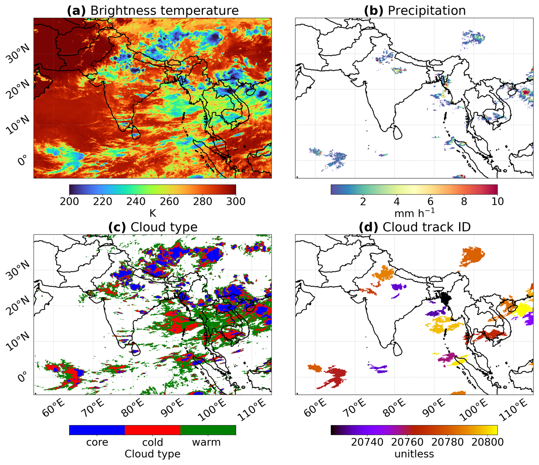
Figure 1 PyFLEXTRKR brightness temperature and precipitation fields reveal widespread deep convection (Tb < 220 K) with $\dot{P}$ > 6 mm h⁻¹ over the Asian monsoon region. Snapshots of pixel-level MCS tracking data on 10 August 2016 over the Asian monsoon region. (a) Brightness temperature [K] highlighting cold cloud tops associated with deep convection, (b) GPM IMERG precipitation [mm h⁻¹] filtered by the pixel-level MCS mask, showing intense rainfall embedded within organized convective systems, (c) Cloud-type classification used by PyFLEXTRKR, distinguishing convective core (blue), cold anvil (red), and warm anvil (green) regions, and (d) Cloud-track ID assigned by the tracking algorithm, illustrating the spatial extent and segmentation of individual MCSs.

2.2.2 MCS Track Statistics

In addition to spatial fields, the PyFLEXTRKR database contains statistics on the structure and evolution of each MCS during its lifetime. For the unique identifier of each tracked system, properties are temporally aggregated to capture the convective lifecycle. The dataset includes lifecycle descriptors (e.g., duration of MCS, start and end epoch time of each track), cloud properties (e.g., area of cold cloud core, area of CCS, minimum Tb in core and cold anvil area), precipitation characteristics (e.g., PF area under CCS, mean and maximum precipitation rate of each PF) and kinematic attributes (e.g., movement speed, movement direction, and centroid position). Additional metrics, such as the size of the cold cloud shield (Tb < 241 K) and the evolution of cloud-top temperature and accumulated precipitation, are recorded at hourly intervals.

2.3 Analysis Period and Precipitation Efficiency Calculation

To calculate MCS ε, we first download PyFLEXTRKR data over the Asian monsoon domain (55°–115° E, 5° S–40° N) from 10 August to 10 September 2016, coinciding with the frequent organized convection during monsoon season (e.g., Virts and Houze, 2016; Paul et al., 2025). This period also corresponds to the DYAMOND Phase I period, so that model evaluation of MCS ε could be performed in a subsequent study. A total of 1321 MCSs were identified from the PyFLEXTRKR database for this period, providing a large sample of monsoonal MCSs. While this period provides a large sample of MCSs, it represents only a single monsoon season and therefore does not capture the full range of interannual variability due, for example, to the El Niño Southern Oscillation (ENSO). Future work could extend the analysis to multiple years spanning different ENSO phases to assess the representativeness of ε characteristics reported here.

To compute ε, we collocated ERA5 LWP and IWP with both pixel-level precipitation fields and the track-level MCS statistics from PyFLEXTRKR. We calculate ε, following Li et al. (2022):

$$\begin{array}{}\text{(1)}& {\mathit{\epsilon }}_{\mathrm{cwp}}={\displaystyle \frac{<\dot{P}>}{<\mathrm{CWP}>}}\frac{\left[\mathrm{kg}{\mathrm{m}}^{-\mathrm{2}}{\mathrm{h}}^{-\mathrm{1}}\right]}{\left[\mathrm{kg}{\mathrm{m}}^{-\mathrm{2}}\right]}\end{array}$$

where $\dot{P}$ is the IMERG surface precipitation rate, CWP is the ERA5 cloud condensate, and the brackets indicate time-averaging. ε is thus calculated from the ratio of time-averaged fields for spatial maps and statistical distributions. For the MCS lifecycle analysis, we also calculate ε at each MCS time step using instantaneous values of $\dot{P}$ and CWP, which we then composite on a normalized lifecycle. Along with ε evaluated with CWP, we also separate values into an ice-partitioned precipitation efficiency, ε_i, using IWP and a liquid-partitioned precipitation efficiency, ε_ℓ, using LWP. We highlight that these ε values represent the $\dot{P}$ produced per unit condensate, rather than an intrinsic microphysical conversion efficiency of ice-to-rain or liquid-to-rain processes. Comparing ε_i and ε_ℓ therefore indicates whether precipitation production is more strongly associated with the depletion of the ice or liquid condensate reservoir. Because CWP is the sum of LWP and IWP, the ε metrics satisfy harmonic combination:

$$\begin{array}{}\text{(2)}& {\displaystyle \frac{\mathrm{1}}{{\mathit{\epsilon }}_{\mathrm{cwp}}}}={\displaystyle \frac{\mathrm{1}}{{\mathit{\epsilon }}_{\mathrm{\ell }}}}+{\displaystyle \frac{\mathrm{1}}{{\mathit{\epsilon }}_i}},\end{array}$$

3 Results

3.1 MCS versus non-MCS precipitation efficiency across the Asian monsoon area

We first construct the statistical distribution of ε and its phase-partitioned values across MCS tracks (Fig. 2). When averaged over the MCS tracks, ε_cwp has the lowest median value of 11.8 h⁻¹, whereas ε_i and ε_ℓ have median values approximately twice as large (Fig. 2a–c). Because the ε metrics represent $\dot{P}$ normalized by condensate amounts, rather than direct ice-to-rain or liquid-to-rain conversion rates, we always expect ε_i and ε_ℓ to exceed ε_cwp, as IWP or LWP are always smaller than or equal to CWP. As expected, the ε distributions shift rightward for maximum values over the MCS lifecycle – with medians increasing to 31.8 h⁻¹ for ε_cwp, 40.1 h⁻¹ for ε_i, and 43.8 h⁻¹ for ε_ℓ (Fig. 2d–f). These distributions of lifetime-maximum ε are also more positively skewed than those of the lifetime-mean: A very small number of MCSs produce very high precipitation efficiencies during their lifecycle, analogous to the right-skewness commonly observed in precipitation rate distributions.

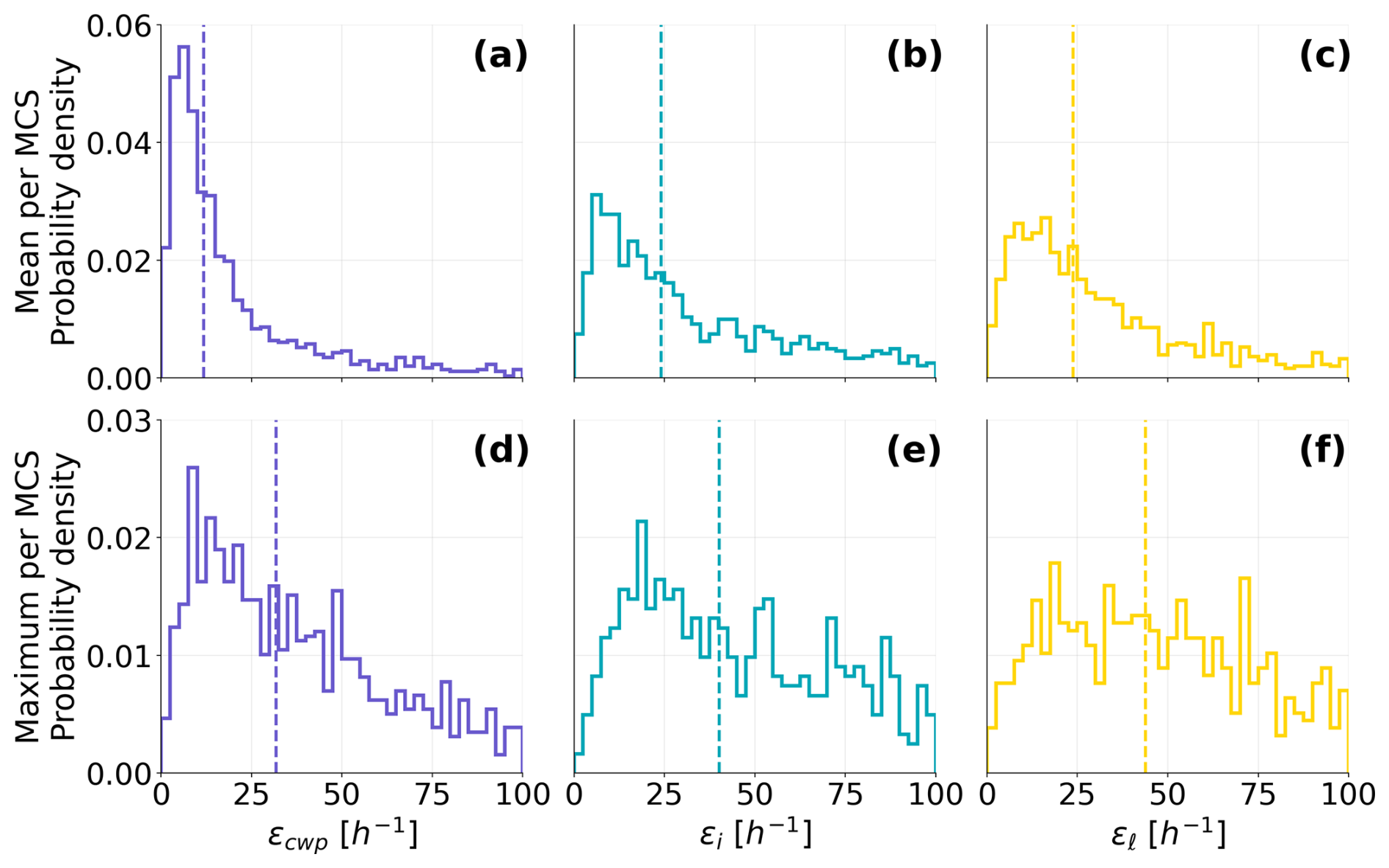
Figure 2 Lifetime-maximum ε is more right-skewed than lifetime-mean values. Probability density functions (PDFs) of ε across MCSs over the Asian monsoon region. Panels (a–c) shows the distributions of ε averaged over each MCS lifetime, while panels (d–f) show the distributions of the lifetime-maximum ε. The three columns correspond to ε_cwp, ε_i, and ε_ℓ, respectively. Dashed vertical lines indicate median values.

We then compare the spatial distribution of ε for MCS versus non-MCS precipitation (Fig. 3). Most grid cells across our domain have a sample size of hundreds of observed MCSs, lending robustness to our spatial patterns (Fig. S1 in the Supplement). We quantify spatial differences with Δε, defined as the difference in MCS versus non-MCS ε. The ratio of MCS to non-MCS ε could also be informative but becomes very large if non-MCS ε is small and may therefore overemphasize certain regions. Across the region and for both overall and phase-partitioned ε, MCSs have values approximately 50 % higher than those of non-MCS convection, with the strongest contrasts occurring over the Bay of Bengal, the Indo-Gangetic Plain, and the South China Sea. The MCS ε_cwp locally exceeds 6 h⁻¹, while that of non-MCS convection typically remains below 3 h⁻¹ (Fig. 3a and d); these values correspond to condensate lifetimes of approximately 10 and 20 min, respectively. The spatial distribution of Δε_cwp further reveals widespread positive differences greater than 1 h⁻¹, extending from the equatorial Indian Ocean through the Bay of Bengal into the South China Sea (Fig. 3g). In these areas, MCSs convert condensate to precipitation two to three times more efficiently than non-MCS convection. Stated another way, MCS cloud condensate is typically converted into surface precipitation within approximately 10 min to one hour, whereas non-MCS condensate may require two to four hours for conversion. This reduction in condensate conversion time within MCSs reflects their accelerated microphysical processing, driven by ascent within their protected updrafts. An exception is a region of low ε east of Sri Lanka, evident in both the MCS and non-MCS fields (Figs. 3 and 5). Because this feature occurs for both MCS and non-MCS ε, it likely reflects environmental conditions, rather than anything microphysical.

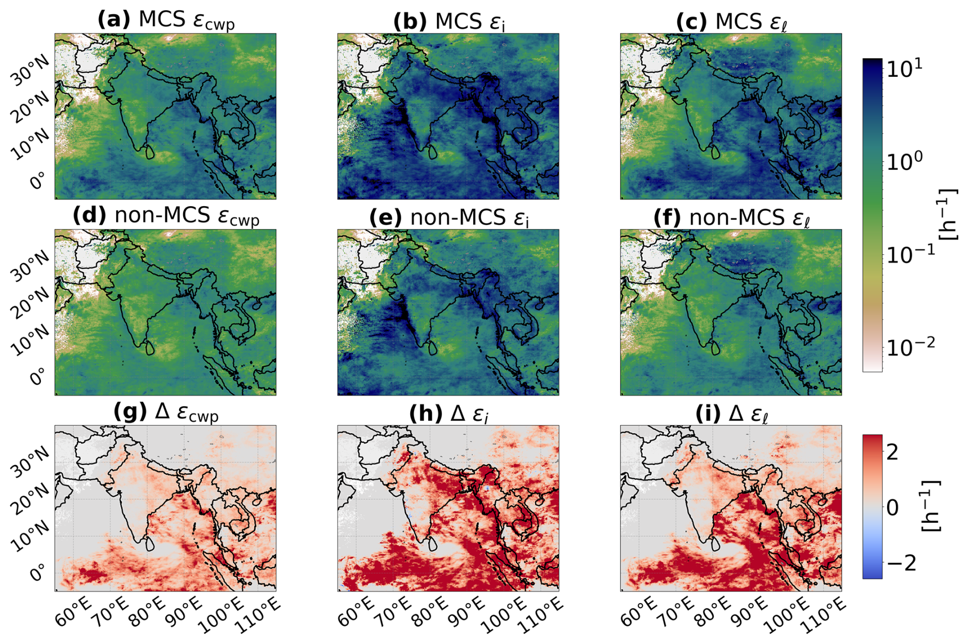
Figure 3 MCSs exhibit much higher ε with mean values 50 % greater than for non-MCS convection across all phases. Spatial distribution of ε metrics over the Asian monsoon region for MCSs and non-MCS convection. The top row (a–c) shows MCS ε based on overall cloud water path (ε_cwp), ice water path (ε_i), and liquid water path (ε_ℓ). The middle row (d–f) presents the corresponding non-MCS precipitation efficiencies, while the bottom row (g–i) shows the MCS-non MCS differences (Δε = ${\mathit{\epsilon }}^{\mathrm{MCS}}-{\mathit{\epsilon }}^{\mathrm{non}-\mathrm{MCS}}$).

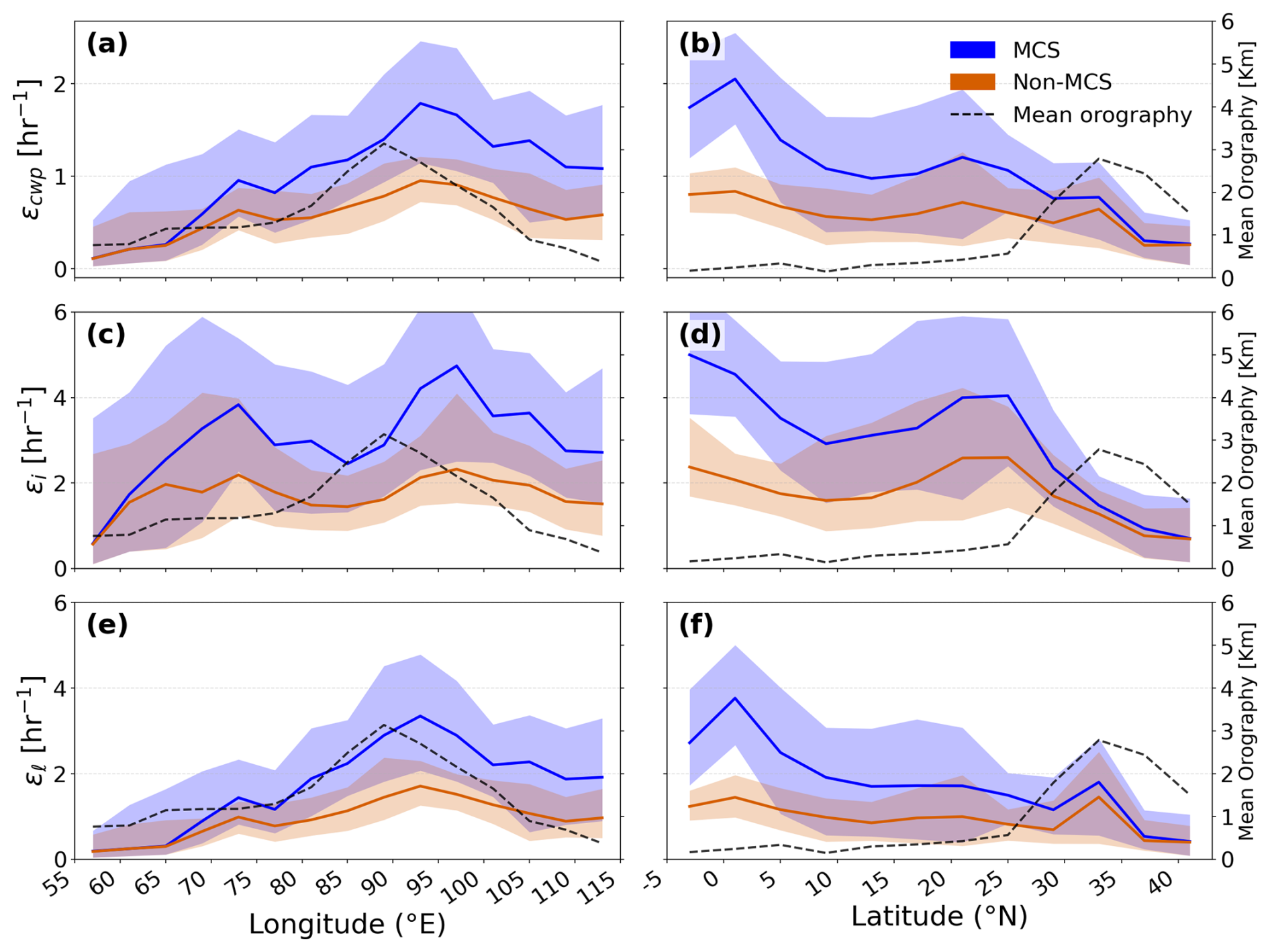
Figure 4 ε tends to increase from west to east and from north to south across our domain, especially in the ice phase. Longitudinal (left column) and latitudinal (right column) variability of ε over the Asian monsoon region for Mesoscale Convective Systems (MCS; blue) and Non-MCS (orange). Rows show (a–b) total precipitation efficiency based on column water path, ε_cwp, (c–d) ice-phase efficiency, ε_i, and (e–f) liquid-phase efficiency, ε_ℓ. Solid lines denote the median ε within longitude or latitude bins, while shaded envelopes indicate the interquartile range (IQR; 25th–75th percentiles), representing the spread of grid-cell values within each bin. The dashed black line (right axis) shows the mean orography within each longitude or latitude bin, providing geographical context for interpreting the influence of major topographic features on the spatial variability of ε.

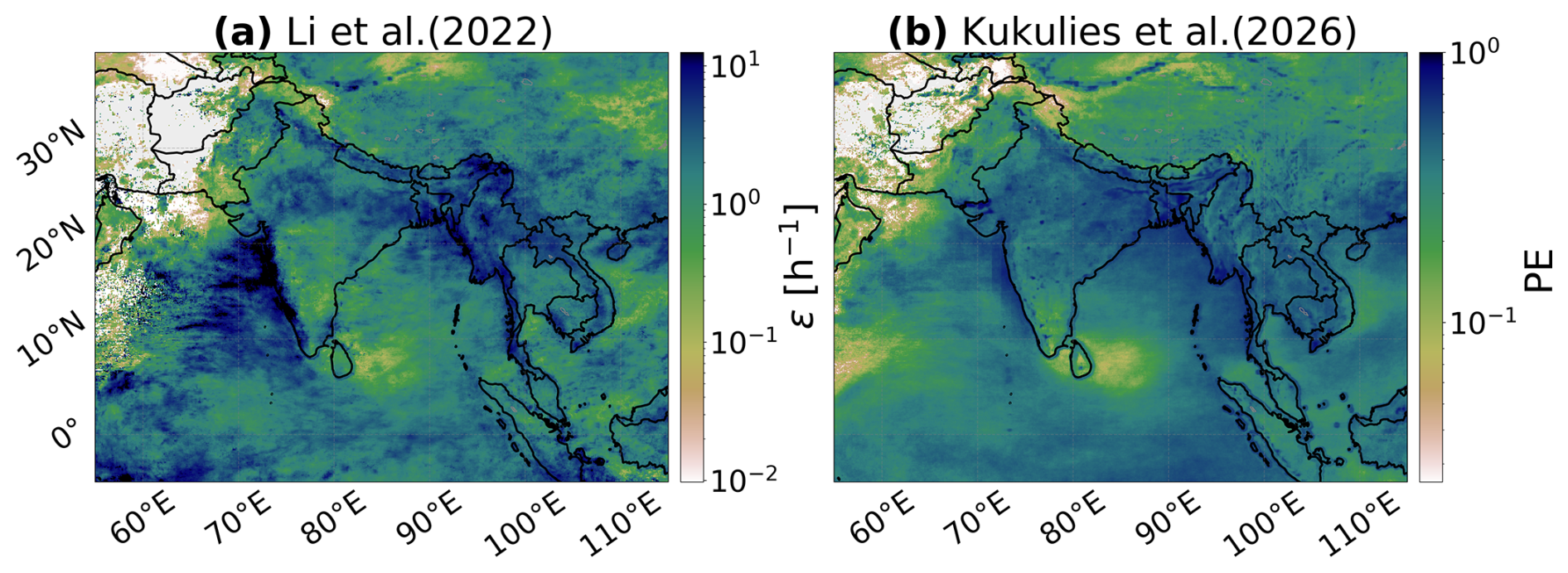
Figure 5 Similar spatial patterns across two independent ε formulations provides confidence in the robustness of our results. Spatial distribution of ε over the Asian monsoon region. (a) Li et al. (2022) ε formulation, expressed as an index (h⁻¹), and (b) Kukulies et al. (2026) PE formulation, expressed as a dimensionless fraction bounded between 0 and 1. A statistically significant Spearman rank correlation (ρ≈0.6; p≪0.01) indicates strong spatial similarity between the two formulations.

To further elucidate which processes generate Δε, we also examine the phase-partitioned efficiencies. ε_i is two- to four-fold larger than ε_ℓ for most MCSs, reflecting that $\dot{P}$ is associated with comparatively smaller amounts of ice condensate or shorter ice condensate lifetimes (Fig. 3b and c). The enhanced ε_i along eastern coastal regions, including areas bordering the Bay of Bengal, South China Sea, and Maritime Continent may reflect the combined influence of abundant moisture supply, frequent deep convection, and efficient mixed-phase precipitation processes. The humid maritime environment likely suppresses sub-cloud evaporation, allowing a greater fraction of precipitation generated per unit IWP, thereby contributing to elevated ε_i. The same increase of ε_i relative to ε_ℓ characterizes non-MCSs. The corresponding non-MCS ε_i and ε_ℓ are substantially smaller, approximately 50 % lower than the MCS equivalents across the domain. Area-weighted mean enhancements over our domain show larger MCS–non MCS contrasts for ε_i than for ε_ℓ: The domain mean Δε_i is 1.4 h⁻¹ versus 1.1 h⁻¹ for Δε_ℓ. The spatial coverage of Δε greater than 0.5 h⁻¹ is also 60 % for the ice phase and only 52 % for the liquid phase (Fig. S2). Looking at these phase-partitioned MCS-non MCS differences statistically, across all metrics high ε greater than 6 h⁻¹ occurs much more frequently in MCSs and particularly for the ice-phase component (Fig. S3).

3.1.1 Dependence on longitude and latitude

While the spatial maps highlight regions of larger and smaller MCS ε, they do not fully reveal how these efficiencies evolve over the west–east monsoon moisture gradient or the north–south land–ocean contrasts. A large-scale west-to-east increase in atmospheric moisture characterizes the Asian summer monsoon area, with drier conditions over the Arabian Sea and higher moisture over the Bay of Bengal, South China Sea, and Maritime Continent. This gradient arises from the transport of warm, moisture-rich air by the summer monsoon circulation and provides a favorable environment for progressively deeper convection toward the eastern part of the domain (Webster et al., 1998; Zhang et al., 2004; Ding and Chan, 2005; Zhou and Yu, 2010; Wang et al., 2021). The strength and position of the moisture gradient vary on synoptic and intraseasonal timescales, but over the one-month period of our study, the gradient remains a persistent feature.

To characterize the effect of these variations on the ε metrics, we evaluate their longitudinal and latitudinal dependences. For each degree longitude, ε values represent all grid cells located along that longitude, i.e., “60° E” includes all grid cells along 60° E across the domain latitudes. The same approach is applied for degrees latitude. We again confirm robust MCS sample sizes across our longitudinal and latitudinal range, with 𝒪(10⁶) occurrences per degree (Fig. S4). Longitudinally, the median ε_cwp increases from 0.2 h⁻¹ over the western Arabian Sea to 1.8 h⁻¹ over the Bay of Bengal (Fig. 4a). A similar eastward increase is evident for non-MCS convection, although with consistently lower values. This increase is consistent with progressively greater atmospheric moisture availability, warmer sea surface temperatures, enhanced deep convection, and more frequent MCS activity toward the eastern monsoon region. The phase-partitioned metrics show that ε_i exhibits the strongest longitudinal variability (Fig. 4c), whereas ε_ℓ displays a weaker but similar eastward increase (Fig. 4e). Local departures from the overall eastward trend coincide with major mountain ranges, suggesting that topography further modulates precipitation efficiency through orographic lifting and condensate retention.

Latitudinally, ε_cwp generally decreases from the equatorial region toward higher latitudes, consistent with reductions in atmospheric moisture and deep convective activity away from the tropical monsoon belt (Fig. 4b). A secondary maximum between 15° N and 25° N coincides with the monsoon rainband and regions strongly influenced by orography, including the Western Ghats and the southern margins of the Tibetan Plateau. ε_i shows the largest land–ocean contrast, whereas ε_ℓ follows a similar but more gradual meridional decrease. Across all latitude and longitude bins, MCSs consistently exhibit higher ε than non-MCS convection, with the largest differences occurring for the ice-phase component.

3.1.2 Dependence on precipitation efficiency metric

Before discussing how ε metrics change with MCS characteristics, we close this section by examining sensitivity of our spatial results to the definition of ε. In Fig. 5, we present maps of precipitation efficiency using an alternate definition recently developed by Kukulies et al. (2024) in which efficiency is defined as the ratio of surface precipitation to the sum of surface precipitation and the positive tendency of IWP, such that only periods of ice condensate growth are considered:

$$\begin{array}{}\text{(3)}& \mathrm{PE}\cong {\displaystyle \frac{\dot{P}}{\left(\dot{P}+{\left.{\displaystyle \frac{\mathit{\delta }\mathrm{IWP}}{\mathit{\delta }t}}\right|}_{[>\mathrm{0}]}\right)}}\end{array}$$

where ${\left.{\displaystyle \frac{\mathit{\delta }\mathrm{IWP}}{\mathit{\delta }t}}\right|}_{>\mathrm{0}}$ represents the positive tendency of IWP, accounting only for cloud ice growth because loss processes such as melting, sublimation, and advection were found to be partially offset by concurrent source terms within the bulk budget (Kukulies et al., 2024). The latter term is an approximation of the condensation rate and therefore PE is dimensionless. IWP is used from the CCIC retrieval (see Sect. 2.1), offering a more observation-based estimate than reanalysis products, where condensate fields depend on microphysical and convective parameterizations. A limitation of this approach is that only the ice phase is considered, implicitly assuming that ice processes dominate precipitation production in deep convective systems. While this formulation differs from Li et al. (2022) in that it defines a dimensionless precipitation efficiency (PE) by relating surface $\dot{P}$ to derived condensation rates, we can nevertheless compare the spatial patterns from both approaches to assess whether the metrics capture the same dominant spatial patterns of condensate-to-precipitation conversion. We do not compute both MCS and non-MCS efficiencies in this comparison.

Despite differences in datasets and physical formulation between Li et al. (2022) and Kukulies et al. (2026), the large-scale spatial distributions of ε are quite similar across the Asian monsoon region (Spearman rank correlation – ρ≈0.6, p≪0.01). Similar features, including elevated efficiencies over the Bay of Bengal and Himalayan foothills and reduced efficiencies near the southern tip of India, appear across both definitions. One notable difference occurs over the Arabian Sea, where the Li et al. (2022) formulation exhibits a more pronounced region of high ε_i than the Kukulies et al. (2026) definition. This discrepancy likely reflects the inclusion of the condensate tendency term, $\frac{d\left(\mathrm{IWP}\right)}{\mathrm{d}t}$, in the Kukulies et al. (2026) formulation, which reduces PE in regions where condensate is simultaneously accumulating and precipitating. This agreement supports the robustness of our spatial analysis and lends confidence to the use of the Li et al. (2022) ε definition in this study.

3.2 Precipitation efficiency across MCS regions

Having established the geographic characteristics of MCS versus non-MCS ε, we next investigate how ε is distributed across regions of the MCS – core, warm anvil, and cold anvil – and across MCSs of different structure. As outlined in Sect. 2.2.1, the core has coldest Tb ≤ 225 K, followed by the cold anvil with warmer Tb between 225 and 241 K and then the the warm anvil with Tb between 241 and 261 K. Together, these thresholds separate intense convective updrafts from layered anvil outflow in MCSs.

Warm anvils occur in 94.1 % of the MCS tracks represented in the cloud-type dataset but occupy only 1.67 % of the total classified MCS cloud area, compared to 53.06 % for cold anvils and 45.27 % for convective cores. Their median contribution at the individual-track level is 1.46 % (interquartile range: 0.74 %–2.61 %). The warm-anvil fraction in the snapshot in Fig. 1c is 1.82 %, close to the value of the entire period, indicating that the snapshot is typical of the study period. Thus, warm anvils occur in most MCSs but generally cover only a small portion of their tracked cloud shields. This limited coverage partly reflects the tracking framework, which includes only warm-cloud pixels associated with identified MCS objects; a thin or semitransparent cirrus outside the tracked cloud shield is not included. However, the warm-anvil ε distributions are based on 248 703 pixel-time observations, and the bootstrap confidence intervals in Table 1 indicate that the aggregate estimates are well constrained. However, because warm anvils are less extensively sampled than cold anvils and convective cores, their ε results should be interpreted more cautiously.

Table 1 Median values and 95 % bootstrap confidence interval (CI) of MCS ε metrics, stratified by MCS region (core, cold anvil, and warm anvil) and ice versus liquid phase. The corresponding condensate residence time is shown in minutes.

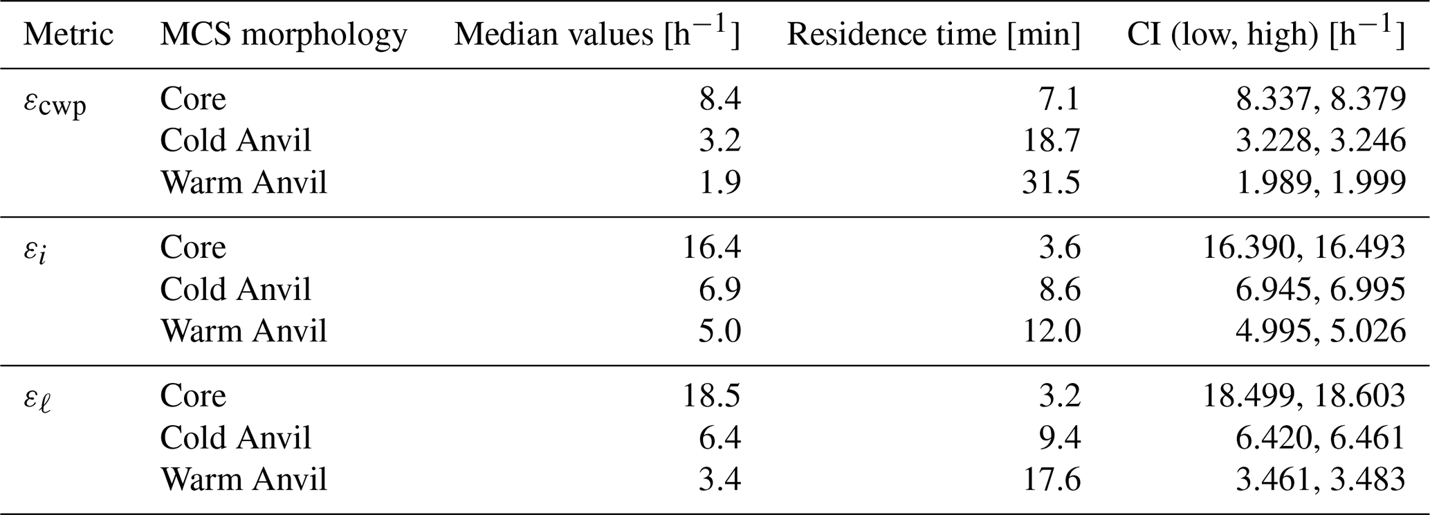
We begin by examining ε_cwp across the three MCS regions. Across all regions, ε_cwp ranges from 0.1 up to 100 h⁻¹, with the core dominating the high-efficiency tail of the distribution (Fig. 6a). These ε_cwp values correspond to a spread in condensate conversion timescale from only a few minutes (ε_cwp ≥ 10 h⁻¹) up to ∼ 10 h. The lower ε_cwp values within the warm and cold anvil regions are reflected in median values of 3.2 and 1.9 h⁻¹, respectively, compared to 8.4 h⁻¹ in the core (Table 1), indicating that anvil efficiencies are approximately 60 %–80 % smaller than core values. Stated in terms of residence time, condensate stays within the anvil three to ten times longer than within the core. This behavior is consistent with strong updrafts, rapid condensate production, and highly efficient ice–liquid conversion within the core of convective towers and weaker ascent and reduced condensate production in the stratiform outflow regions.

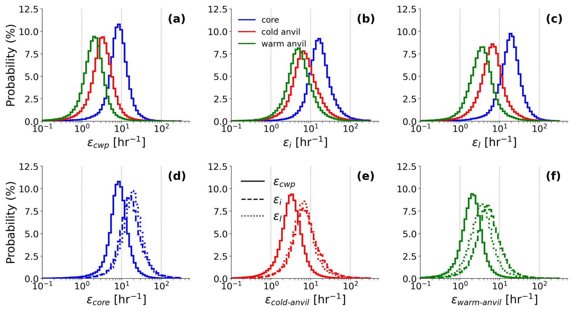
Figure 6 The core consistently has the highest ε values, followed by the cold and then warm anvils, reflecting the transition from deep convective to stratiform and non-precipitating cloud. Probability distributions of ε across MCS morphologies, defined by Tb thresholds in the FLEXTRKR data. Panels (a–c) show distributions of ε for the convective core (blue), cold anvil (red), and warm anvil (green) regions, computed for (a) overall precipitation efficiency (ε_cwp), (b) ice-phase efficiency (ε_i), and (c) liquid-phase efficiency (ε_ℓ). Panels (d–f) regroup the distributions by MCS region to compare total and phase-partitioned ε within each sector: (d) for the core, (e) for the cold anvil, and (f) for the warm anvil. In panels (d–f), solid lines denote ε_cwp, dashed lines denote ice-phase efficiency (ε_i), and dotted lines denote liquid-phase efficiency (ε_ℓ).

We next phase-partition ε, both to understand whether the core-cold anvil-warm anvil hierarchy exists in the other ε metrics and to determine which phase drives the ε differences across MCS morphologies. The core region still contains the highest ε_i and ε_ℓ; however, the separation in ε_i for cold versus warm anvil is less than the separation in ε_cwp for those regions. The ice-partitioned precipitation efficiency values shift upward by 30 % to 50 % relative to ε_cwp, as established in the previous section. The median of ε_i reaches 16.4 h⁻¹, decreasing to 6.9 h⁻¹ in the cold anvil and 5.0 h⁻¹ in the warm anvil. The difference of ε_cwp across anvil types is mainly determined by the contribution of ε from the liquid phase. This is consistent with recent modeling study showing that warm-rain and ice-phase pathways coexist in deep convection, and that their relative contributions to precipitation depend on the efficiency of condensate-to-precipitation conversion processes (e.g., autoconversion, riming, aggregation), rather than cloud depth alone (Gupta et al., 2023). Taken together, these distributions of ε across MCS morphologies show that the convective core generates precipitation about four times more efficiently than the warm anvil and two times more efficiently than the cold anvil, with the liquid phase determining much of the ε differences across the warm and cold anvil regions.

To understand the difference in warm versus cold anvil ε_cwp, we visualize the distributions of $\dot{P}$ versus CWP across the MCS morphologies (Fig. S5). When min-max normalizing both $\dot{P}$ and CWP, there is greater overlap between these distributions in the warm anvil region than in the cold anvil region. In other words, the difference between condensate amounts aloft and sedimenting is more pronounced in the cold anvil than the warm anvil. Physically, warm anvils are typically characterized by weak vertical velocities, small droplet and ice crystal sizes, and limited microphysical growth via riming, aggregation, or collision–coalescence. Consequently, condensate within warm anvils is predominantly retained in non-precipitating form, resulting in inefficient rainfall production. In contrast, cold anvils, although located at higher altitudes, remain more directly connected to active convective regions and contain recently detrained ice condensate that is still influenced by ongoing ice-phase growth processes (e.g., aggregation, riming, and depositional growth). Cold anvils therefore favor more efficient growth and aggregation of ice particles, leading to the formation of precipitation-sized hydrometeors that sediment through the melting layer and contribute to stratiform rainfall at the surface (Yuter and Houze, 1995; Houze, 2014). By comparison, warm anvils generally represent older and more horizontally dispersed cloud outflow, where weaker vertical motions and longer condensate residence times promote condensate retention and sublimation rather than precipitation production (Barnes and Jr, 2014; Houze, 2014). Consequently, a smaller fraction of condensate in the warm anvil is converted into surface precipitation, resulting in lower precipitation efficiency. The reduced ε_cwp of the warm anvils therefore reflects microphysical inefficiency rather than longer residence times alone, highlighting that the large loading of condensate does not imply efficient precipitation production.

We lastly reorganize the ε distributions by MCS sector to more clearly see the differences across condensate phase (Fig. 6d–f). While ε_i generally exhibits large values, the relative ordering of ε metrics is not consistent across MCS regions. Instead, the dominant efficiency shifts from liquid-phase processes in the core to ice-phase processes in the warm anvil, with substantial overlap among metrics in the cold anvil. Rather than indicating a universal hierarchy, these results show that no single microphysical process dominates precipitation production across all MCS regions. Instead, the slightly higher ε_ℓ in the convective core suggests shorter liquid condensate residence times there, while ε_i becomes relatively more prominent in the warm-anvil region. The cold anvil exhibits substantial overlap among phase-partitioned efficiencies, consistent with mixed microphysical processes. Together, these patterns suggest that anvil regions, particularly the warm anvil, function primarily as reservoirs of condensate rather than regions of continuous precipitation production. This interpretation is supported by the relatively low ε in the warm anvil, indicating longer condensate residence times and slower conversion of condensate to precipitation.

Dependence on MCS extent and depth

Next, we investigate how ε changes with MCS morphology, in particular with the extent and depth of the MCS. MCS area refers to the contiguous cold cloud cover in PyFLEXTRKR (see Sect. 2.2.1). MCS depth is defined as the vertical extent of the cloud system, inferred from the minimum infrared Tb associated with the convective core and stratiform regions, with colder cloud-top temperatures indicating deeper convection. We examine the scaling relationships between ε and MCS area and depth as a function of lifetime mean and maximum rain rates. These scalings include all stages of systems that eventually satisfy the MCS criteria; MCS areas smaller than the threshold therefore correspond to convective growth prior to attaining MCS status (Fig. 7). All ε metrics increase with MCS area for areas less than ∼ 24 km² (Fig. 7). All three efficiency metrics exhibit statistically significant, strong positive correlations between the mean $\dot{P}$ and MCS area in this range, with r values of 0.98 across the metrics ($p<{\mathrm{10}}^{-\mathrm{4}}$, Fig. 7a, Table S1). Among the phase-partitioned ε metrics, ε_i increases most rapidly with area, reaching a peak value of 30 h⁻¹ for an MCS area of 24 km² before decreasing for the largest areas. ε_ℓ increases more slowly with MCS area before plateauing at a value of 20 h⁻¹ for the largest systems. As a combination of the ice- and liquid-phase scalings, ε_cwp also increases with MCS area up to a threshold beyond which it declines slightly. This threshold area of 24 km² corresponds to an MCS effective diameter of 160 km. The non-monotonic behavior of the ε–area scalings, most pronounced for ε_i, likely reflecting a disproportionate increase in system-integrated IWP relative to $\dot{P}$ at the largest MCS sizes, such that the accumulation and storage of condensate in extensive stratiform and anvil regions outpaces the corresponding increase in $\dot{P}$.

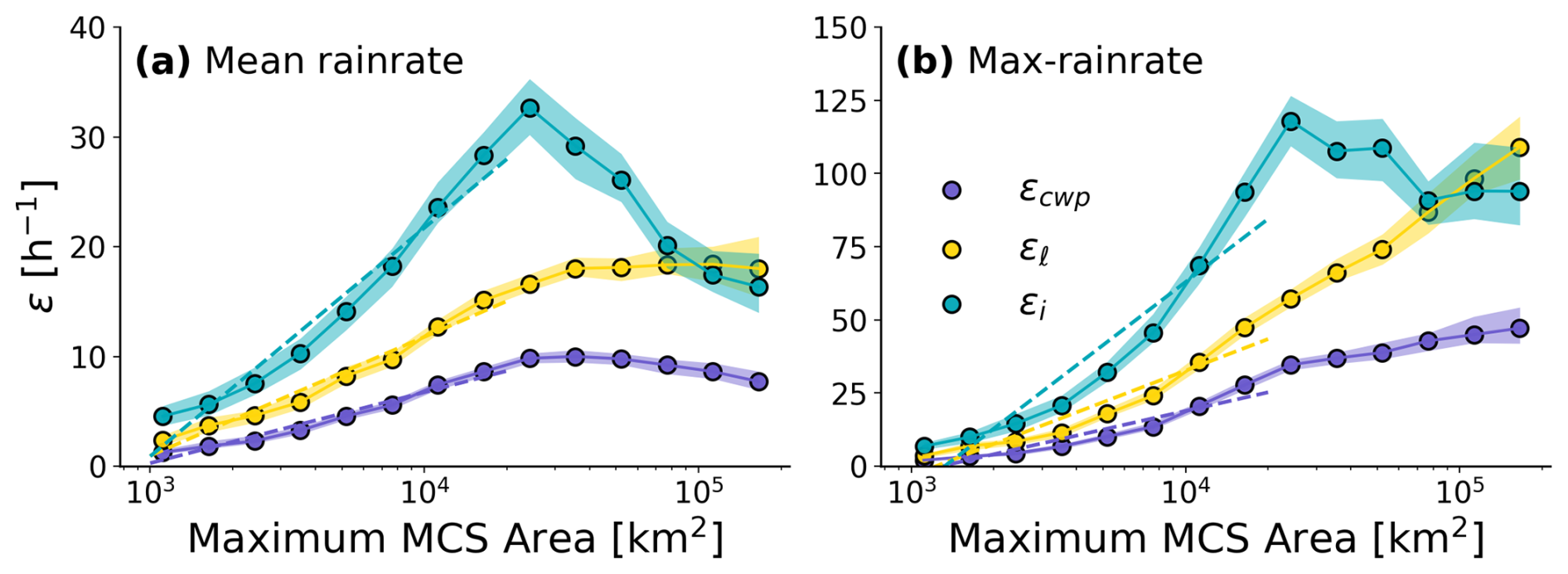
Figure 7 For both mean and maximum rain rates, ε increases with MCS size for areas less than 24 km². Scalings of the ε metrics versus MCS area for (a) lifetime mean rain rate and (b) lifetime maximum rain rate. The MCS area shown represents the full tracked evolution of PyFLEXTRKR systems, including stages before they satisfy the MCS identification criteria (minimum precipitation-feature area of 44 km²). Consequently, areas smaller than 44 km² correspond to the developing stages of systems that subsequently evolve into MCSs. Curves show the total precipitation efficiency (ε_cwp, purple), liquid-phase efficiency (ε_ℓ, yellow), and ice-phase efficiency (ε_i, cyan). Dashed lines indicate log–linear fits to the ε–area relationship, computed only for MCS areas smaller than 2×10⁴ km². Shading indicates the 95 % bootstrap confidence interval on the binned median ε metrics within each MCS-area bin.

Scalings of the lifetime maximum $\dot{P}$ against MCS area also increase up to a threshold area but with weaker log-linear correlations (Fig. 7b). Correlation coefficients are now 0.95 across the three epsilon metrics but still with statistical significance ($p<\mathrm{5}\times {\mathrm{10}}^{-\mathrm{4}}$). In contrast to the mean $\dot{P}$ scalings, there is no decrease in ε_ℓ beyond a certain MCS area. ε_ℓ continues to increase for the largest MCS extents and becomes comparable to or exceeds ε_i, indicating that large systems achieve high peak rain rates through both ice and liquid-phase processes. These scalings demonstrate that MCS area strongly controls ε, with larger MCSs more efficiently converting cloud condensate into precipitation but only up to a certain point.

We next examine the sensitivity of the ε metrics to the MCS depth across mean and max rain rates (Fig. 8). ε_cwp, ε_ℓ, and ε_i increase systematically with decreasing Tb, which corresponds to increasing MCS depth. In other words, deeper MCSs more efficiently convert cloud condensate into surface precipitation. The correlation coefficient for these scalings reaches −0.97 across all ε metrics with greater than 99 % statistical significance, indicating that more than 95 % of the variance in ε can be explained by variations in the MCS cloud-top temperature (Table S2). ε_i increases by more than 150 % between the warmest and coldest Tb (Fig. 8a). ε_ℓ also doubles across the Tb range. As for extent, we also scale the maximum $\dot{P}$ against MCS depth. The correlation between the ε metrics and Tb remains quite robust with statistically significant coefficients of −0.99 ($p<{\mathrm{10}}^{-\mathrm{5}}$). These near-perfect correlations indicate that the intensity of the maximum rainfall is tightly coupled with the vertical development of the MCSs. ε_i is consistently most sensitive to Tb; however, there is no decrease in ε_i for the deepest MCSs as there was for the largest MCSs. Unlike the ε–area scalings, ε metrics does not show the non-monotonic behavior with increasing MCS depth. Increases in ε metrics with depth primarily reflect dynamical intensification (e.g., stronger updrafts driven by larger CAPE or reduced entrainment) rather than a requisite increase in total condensate. Because deeper systems do not necessarily accumulate condensate aloft, the ε metrics do not decrease at the largest depths. The contrast between these scalings highlights distinct controls on ε metrics associated with horizontal versus vertical MCS growth.

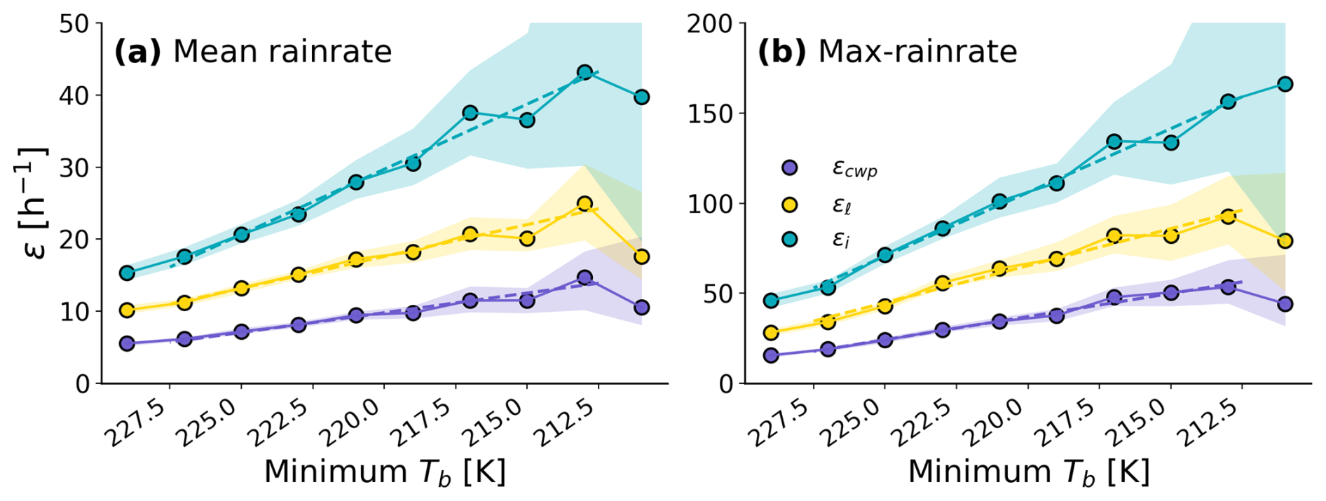
Figure 8 For both mean and maximum rain rates, ε increases as brightness temperature decreases, indicating that deeper convection more effectively converts condensate to rainfall. Scalings of the ε metrics versus cloud-top brightness temperature for (a) lifetime mean rain rate and (b) lifetime maximum rain rate. Curves show the total efficiency (ε_cwp, purple), liquid-phase efficiency (ε_ℓ, yellow), and ice-phase efficiency (ε_i, cyan). Dashed lines indicate log–linear fits to the ε–depth relationship, and shading indicates the 95 % bootstrap confidence interval on the binned median ε metrics within each Tb bin.

3.3 Precipitation efficiency over the MCS lifecycle

We next look at the evolution of ε metrics over the MCS lifecycle. The MCS lifecycle is normalized by rescaling the system lifetimes to a common 0–1 interval, where 0 and 1 correspond to initiation and dissipation according to the FLEXTRKR tracking, respectively. We first use this normalized lifecycle to understand changes in MCS area, Tb, and $\dot{P}$ (Fig. S6). While mean and maximum $\dot{P}$ peak about 25 % and 35 % of the way through the lifecycle, respectively, minimum Tb occurs about 42 % and maximum extent at about 58 % of the lifecycle. From these properties, systems are mature in the middle third of their normalized lifecycle (0.3–0.6), when convection is deepest and system extent is largest. All three ε metrics show a lifecycle dependence with rapid increases during the early growth stage and more gradual decreases during development and dissipation (Fig. 9). Increases in ε metrics occur within the first 20 % of the lifecycle, while the decreases occur over the remaining 80 % during the decay-phase behavior of condensate production. This evolution closely resembles the MCS ε lifecycle reported by Kukulies et al. (2026) (their Fig. 4b), who found increasing efficiency from initiation to maturity followed by decreasing efficiency from maturity through decay in kilometer-scale simulations and satellite-based estimates. In our observations, peak ε occurs slightly earlier in the normalized lifecycle than in Kukulies et al. (2026). As noted above, mean and maximum $\dot{P}$ peak early in the lifecycle, while minimum cloud-top temperatures and maximum system area peak later. ε thus reaches its highest values at the same time as $\dot{P}$, rather than at the same time as system depth or extent.

Phase partitioning further refines this evaluation over the lifecycle. The high values of ε_i throughout most of the lifecycle align with a central role for ice-phase growth and sedimentation in sustaining efficient rainfall during mature MCS stages. Apart from the hierarchy of magnitudes, the lifecycle behavior of ε is quite consistent across all metrics, indicating that phase partitioning plays a secondary role in controlling variations of ε over the lifecycle. We also refine the ε values over lifecycle for short (4–8 h), medium (8–12 h), and long-lived (> 12 h) systems (Fig. S7). These lifetime classes were selected to represent distinct stages of MCS longevity while ensuring sufficient numbers of systems within each category for robust composite statistics. For each system, the lifecycle was normalized from initiation to dissipation, interpolated onto a common set of normalized lifecycle bins, and then composited within each lifetime class (Fig. S7). The normalized lifecycle of ε is qualitatively similar across all lifetime classes, with elevated values during development and maturation followed by decline during dissipation. The lifecycle behavior discussed above should therefore be robust across MCSs with different absolute lifetime.

This evolution of ε over the lifecycle is consistent with our scalings in the previous section, as MCS growth and maturation are characterized by expanding system coverage and progressively colder cloud tops, both of which are associated with enhanced ε. In contrast, the late-stage decline in all efficiency metrics coincides with a shrinking system area and a warming of the cloud tops, indicating reduced vertical depth, weaker dynamical organization, and diminished microphysical conversion efficiency. Of course, evolution of ε is not tied solely to area. While our lifecycle analyses follow temporal evolution of systems, the scalings between ε and MCS area are statistical relationships, and smaller systems may occur either during growth or dissipation. Together, these results demonstrate that the observed lifecycle modulation of ε reflects the coupled evolution of storm size, cloud-top height, and microphysics, with ice-phase processes playing a dominant role during periods of maximum system extent and minimum cloud-top temperature.

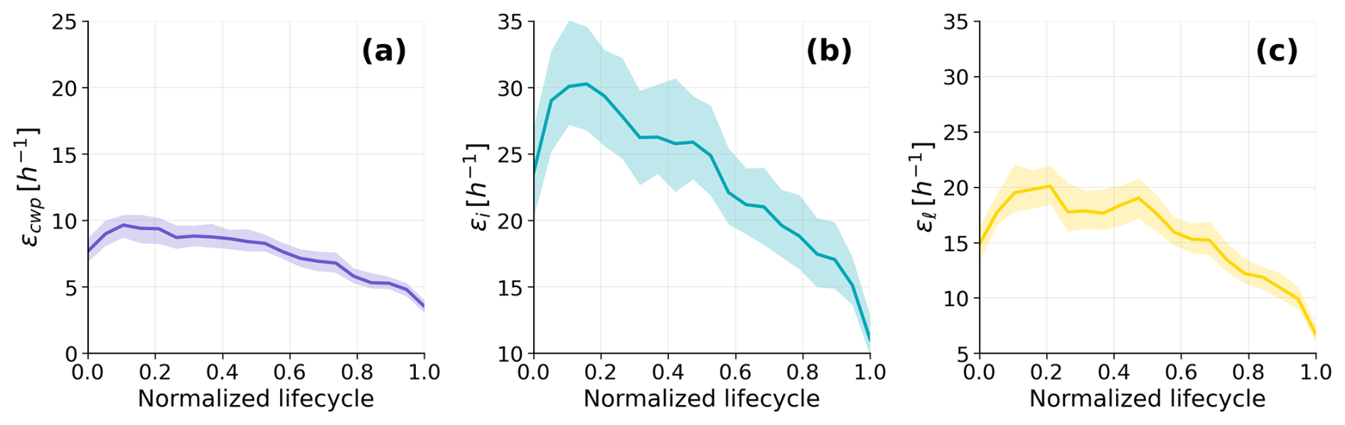
Figure 9 The ε metrics peak within the first 20 % of MCS lifecycle. ε metrics computed as a function of normalized MCS lifetime, where 0 indicates system initiation and 1 indicates system dissipation, for (a) ε_cwp, (b) ε_i, and (c) ε_ℓ. Each curve represents the average ε across all tracked MCSs, and shading represents the 95 % bootstrap confidence interval on the median ε metrics across MCS tracks at each normalized lifecycle phase. Note that y-axis limits change between panels but have a consistent range of 25 h⁻¹.

4 Conclusions

Accurately representing precipitation associated with mesoscale convective systems (MCSs) remains a major challenge for climate models. Our recent evaluations of DYAMOND storm-resolving simulations against GPM IMERG observations over a South Asian domain show that the largest model–observation precipitation differences occur in regions dominated by frequent MCS activity, including the southern Indian Ocean and the Bay of Bengal (Makgoale and Sullivan, 2025). In these regions, rainfall is primarily produced by organized deep convective systems in which surface precipitation ($\dot{P}$) is strongly regulated by storm morphology, lifecycle, and microphysical processes, meaning that modeled precipitation rates are particularly sensitive to deficiencies in MCS representation. Motivated by these findings, this study provides a comprehensive observational assessment of the efficiency of precipitation production (ε) in MCSs over the Asian Monsoon Region. We analyze PyFLEXTRKR MCS track statistics and pixel-level diagnostics in combination with ERA5 cloud condensate fields to characterize ε of 1321 MCSs over the Asian monsoon region from 10 August to 10 September 2016 using the Li et al. (2022) index, defined as the ratio of $\dot{P}$ to CWP. We note that ERA5 condensate fields are derived from a data-assimilating forecast model and therefore depend on model microphysical parameterizations. As such, uncertainties in condensate partitioning and phase representation may influence ε estimates.

Our results show that for both overall efficiency (ε_cwp) and ice and liquid phase-partitioned efficiencies (ε_i and ε_ℓ) MCSs convert cloud condensate into surface precipitation about 50 % more efficiently than non-MCS convection. Spatial distributions in the ε metrics across the Asian monsoon region further indicate enhanced efficiency in moisture-rich, dynamically favorable environments and reduced efficiency in regions characterized by limited moisture supply, weaker convective organization, or continental interiors. Strong enhancements in MCS ε also occur along the Himalayan foothills. Phase-partitioned analyses reveal that ε_i systematically exceeds ε_ℓ in both MCS and non-MCS regimes and drives more of the MCS versus non-MCS differences. In contrast, lifecycle evolution in ε – characterized by a rapid increase during early growth and more gradual decreases during development and dissipation – is largely phase independent. The decline in ε during dissipation stages reflects continued condensate storage within stratiform and anvil regions while surface precipitation weakens.

Another key result of this study is the systematic variation of ε across MCS regions from the core to the cold and warm anvils. Decomposing ε by MCS region shows that the convective core consistently has the highest efficiency across all ε metrics, corresponding to short condensate residence times on the order of a few minutes, whereas warm anvils display the lowest efficiencies, with condensate retained for several hours before contributing to surface precipitation. Efficiency differences between cold and warm anvils are driven by differences in liquid-phase condensate more than by those in the ice phase. Scaling ε by MCS area and depth further clarifies the factors controlling rainfall production. The non-monotonic relationships between ε and MCS area reflect the disproportionate growth of system-integrated ice condensate associated with anvil expansion in the largest systems, such that condensate accumulation outpaces increases in surface precipitation. In contrast, ε increases monotonically with MCS depth, consistent with depth increases being driven primarily by dynamical intensification (e.g., stronger updrafts or reduced entrainment) rather than excess condensate storage. This distinction highlights fundamentally different roles of horizontal and vertical storm growth in regulating ε.

Overall, our findings are consistent with previous studies discussed in the Introduction that emphasize the important role of convective organization, storm morphology, and microphysical processes in regulating ε. In particular, the enhanced ε of MCSs relative to non-MCS convection and the distinct behavior of convective cores and anvils are broadly consistent with previous observational studies of organized convection. Our results also corroborate the ε framework presented by Kukulies et al. (2026) for a different geographical region, suggesting that the links between convective organization, condensate partitioning, and ε are robust across diverse climatic environments.

Potential uncertainties should also be considered when interpreting our results. GPM IMERG $\dot{P}$ estimates are known to exhibit regional biases, particularly over complex terrain and in areas with sparse ground-based observations, while ERA5 IWP and LWP are not directly observed but are inferred through data assimilation and model microphysical parameterizations constrained by satellite and conventional observations. These uncertainties may affect the magnitude of the estimated ε in some regions, particularly over the complex topography of the Asian monsoon domain. Nevertheless, because our analysis focuses on broad spatial patterns and relative differences between MCS and non-MCS convection using a consistent observational framework, we expect the principal conclusions to remain robust.

While this study focuses on the Asian monsoon region, we expect the qualitative contrast in ε between MCS and non-MCS convection to extend to other regions because organized convection generally develops in more humid environments that reduce entrainment and evaporative losses relative to isolated convection. However, the quantitative magnitude and spatial distribution of ε are likely to depend on regional environmental conditions, including moisture availability, large-scale circulation, and topographic influences that are particularly important over the Asian monsoon. The regional context of these spatial patterns is discussed in Sect. 3.1.1. Furthermore, although larger MCSs generally exhibit higher ε, our results suggest that the observed contrast between MCS and non-MCS convection reflects storm organization and its associated dynamical and microphysical processes rather than system size alone.

Recent work indicates that estimates of storm frequency, size, and duration can vary substantially across tracking methodologies (e.g., Prein et al., 2024; Feng et al., 2025). It would be worthwhile to examine how our results change when using other MCS tracking datasets. As noted in the introduction, many definitions of ε exist. We have tested robustness of our spatial analyses to a different PE definition; however, other metrics using microphysical tendencies or moisture convergence could also be tested to compare MCS and non-MCS convection. An important next step is to apply the phase-specific ε diagnostics developed here – including morphology-dependent ε, condensate conversion time estimates, and phase-resolved condensate–precipitation relationships – to storm-resolving model output. This framework enables direct comparison between observed and simulated MCS ε, allowing identification of biases in condensate partitioning, conversion rates, and their dependence on system morphology and lifecycle stage. Such a comparison would provide a rigorous benchmark to evaluate how high-resolution models reproduce the structural, microphysical, and lifecycle-dependent characteristics of MCS ε identified here. In addition, future studies should examine the diurnal and seasonal dependence of ε, both for MCSs and non-MCS convection, as well as its sensitivity to large-scale environmental conditions, including moisture availability, vertical wind shear, and thermodynamic stability. Addressing these aspects will further clarify the physical controls in ε and improve its utility as a diagnostic for model evaluation and climate applications.