Detectability of solid particle injections into the stratosphere with satellite solar occultation instruments

Stratospheric aerosol injections (SAI) have been proposed as a potential climate intervention to mitigate some effects of global warming. This method involves the idea of injecting sulphur dioxide into the stratosphere. Other ideas include the injection of solid particles, like alumina and calcite, as these particles absorb less terrestrial infrared radiation and scatter solar radiation more efficiently. The aim of the study is to investigate the detectability of the continuous injection of 5 Tg yr⁻¹ of alumina and calcite with typical satellite solar occultation instruments using SOCOL-AERv2 (SOlar Climate Ozone Links-Atmospheric and Environmental Research Incorporation version 2) model simulation results and the SCIATRAN radiative transfer model. Vertically resolved retrievals of the stratospheric aerosol extinction coefficient at 565 nm demonstrate that, under the assumptions made, it is possible to detect the injection of solid particles into the stratosphere and that the corresponding SAI signals can be distinguished from natural variability under near-background conditions, which is essential for the observational verification of potential SAI perturbations.

1 Introduction

Stratospheric aerosol injections (SAI) have been proposed as a potential climate intervention to mitigate some of the effects of anthropogenic global warming. The concept involves the injection of aerosol precursors, such as sulphur dioxide, into the stratosphere, where sulphate aerosol particles are formed that scatter part of the incoming shortwave radiation back into space, which can lead to a decrease in the Earth’s globally averaged surface temperature (Budyko, 1977; Crutzen, 2006; Kremser et al. , 2016). The idea originated from observations of the cooling effect of explosive volcanic eruptions where extensive amounts of sulphur dioxide reach the stratosphere. With a typical lifetime of about 1–2 years for stratospheric aerosol particles, the SAI aerosol layer would need to be continuously refreshed to sustain its climate effects. Other ideas include the injection of solid particles, such as alumina (Al₂O₃) and calcite (CaCO₃), as these particles absorb less terrestrial infrared radiation, therefore reduce stratospheric warming compared to the injection of sulphur dioxide, which was shown to reduce detrimental impacts on circulation and climate (Wunderlin et al., 2024; Stefanetti et al., 2024) as well as on the hydrological cycle (Geurts et al., 2026). These solid particles would also scatter solar radiation more efficiently (e.g., Dykema et al., 2016; Vattioni et al., 2024a, 2025) and might reduce impacts on stratospheric ozone compared to the injection of sulphur dioxide (Vattioni et al., 2023, 2025). The improved ability to scatter solar radiation also implies that less stratospheric aerosol loading would be needed (e.g., Weisenstein et al., 2015; Dykema et al., 2016).

However, no prior study has evaluated whether realistic injection scenarios of solid-particle SAI produce extinction signals detectable by existing satellite solar occultation instruments or whether such signals can be distinguished from natural variability. Solar occultation instruments, like SAGE III/ISS (Stratospheric Aerosol and Gas Experiment III, mounted on the International Space Station (ISS)) or the future Atmospheric Limb Tracker for Investigation of the Upcoming Stratosphere (ALTIUS) instrument (Fussen et al., 2019), can potentially be used to detect possible future SAI deployments above a certain injection rate. SAGE III/ISS measures the attenuation of solar radiation caused by scattering and absorption by atmospheric constituents including aerosols, water vapour, nitrogen dioxide, and ozone. The instrument observes approximately 15 sunrises and 15 sunsets within 24 h and provides measurements over a latitude range from 70° S to 70° N (NASA, 2022). Our previous study demonstrated that stratospheric sulphate aerosols formed from continuous injections of 1 and 2 Tg S yr⁻¹ can very likely be detected by a typical satellite solar occultation instrument, even when natural variability is considered (Lange et al., 2025). This study focuses on satellite solar occultation instruments because they measure the attenuation of the direct solar beam and the associated retrievals do not require additional assumptions on, e.g., the aerosol phase function, multiple-scattering contribution, or surface albedo, which are needed for the interpretation of limb-scatter measurements. This keeps the retrieval error analysis comparatively well constrained. Furthermore, this work connects directly to the retrieval framework established in the previous study (Lange et al., 2025) and the adaption of the same instrument concept ensures methodological consistency and comparability between the two studies.

SAI is still subject to substantial scientific and societal debate, in part due to remaining research gaps and uncertainties (e.g., Haywood et al., 2025). At the same time, ongoing climate change and increasing associated damages and costs have led to continued discussion of possible deployment scenarios. SAI is often considered to be relatively inexpensive compared to other climate intervention strategies (e.g., Moriyama et al., 2017), which could increase the interest of private actors. For instance, companies may find SAI to be profitable (e. g. the “Make sunsets” company, Make sunsets, 2026). These developments highlight the importance of being able to detect potential future SAI deployments.

The aim of this study is to investigate whether SAI scenarios based on solid particles, here the injection of 5 Tg yr⁻¹ alumina and calcite, are detectable with typical satellite solar occultation instruments and whether the sensitivity is sufficient to distinguish the SAI signal from natural variability. The injection rate of 5 Tg yr⁻¹ was chosen because it results in an all-sky radiative forcing of about −1 W m⁻² (Vattioni et al., 2025), a reasonable magnitude for an SAI scenario aiming to offset some effects of anthropogenic climate change.

The paper is structured as follows. Section 2 describes the SOCOL-AERv2 model simulations, as well as the transmission calculations and the stratospheric extinction coefficient profile retrievals with SCIATRAN. Section 3 provides an overview of the results, followed by the discussion and conclusions.

2 Methodology

2.1 SOCOL-AERv2

SOCOL-AERv2 (Feinberg et al., 2019) is based on the ECHAM5.4 general circulation model (Roeckner et al., 2003) and is coupled to the chemistry module MEZON (Egorova et al., 2003) and the aerosol microphysics module AER (Weisenstein et al., 2007; Sheng et al., 2015). The longwave (LW) radiative transfer code implemented in ECHAM5.4 uses the Rapid Radiative Transfer Model (RRTM; Mlawer et al., 1997), which applies the correlated k-method across 16 spectral bands spanning wavenumbers from 10 to 3000 cm⁻¹ (corresponding to approximately 3.3–1000 µm). The shortwave (SW) radiative transfer code is handled following Fouquart and Bonnel (1980) with a spectral discretisation of 6 bands between 185 nm and 4 µm. The SW scheme accounts for scattering and absorption of SW radiation, the LW scheme considers absorption and emission of radiation.

The SOCOL-AERv2 model operates with a horizontal resolution of T42 (2.8°×2.8°) and 39 vertical sigma-pressure levels extending to 0.01 hPa (approximately 80 km altitude). Model dynamics are calculated at 15 min intervals. Chemical processes are solved every 2 h and include a 2 min internal time step to resolve aerosol microphysics (Vattioni et al., 2024b). The model simulates the injection and transport of solid particles as well as their microphysical processes (Vattioni et al., 2024c). These include settling, agglomeration through self-coagulation, interactions with sulphuric acid aerosols via coagulation, condensation of sulphuric acid (H₂SO₄) on particle surfaces, and settling of the solid particles. The solid particles are interactively coupled to the model’s radiation and heterogeneous chemistry schemes (Vattioni et al., 2024c). Furthermore, heterogeneous reactions on the solid particle surfaces are considered as well as the interaction of the solid particles with shortwave and longwave radiation based on their scattering and absorption cross sections (Vattioni et al., 2024c). Alumina particles acquire an H₂SO₄–H₂SO₄ coating through condensation of gaseous H₂SO₄ and coagulation with aqueous H₂SO₄ droplets (Vattioni et al., 2025). Since Vattioni et al. (2023) found a contact angle of about 30°, this coating likely does not cover the alumina surface completely, the bare alumina surface remains available for heterogeneous reactions beyond those occurring on sulphuric acid (Vattioni et al., 2025): ClONO${}_{\mathrm{2}}+\text{HCl}\stackrel{\text{surf}}{⟶}{\text{Cl}}_{\mathrm{2}}+{\text{HNO}}_{\mathrm{3}}$. For the calcite particles different heterogeneous reactions are important, involving the reaction with hydrochloric acid (HCl), nitric acid (HNO₃), and sulphuric acid (H₂SO₄) (Vattioni et al., 2025). For that, the best currently available estimates of the uptake coefficients were applied (Vattioni et al., 2025). A comprehensive description of the solid particle microphysics module implemented in SOCOL-AERv2 can be found in a previous study (Vattioni et al., 2024c). The scattering and absorption cross sections for the solid particles were calculated using a semi-empirical code (Rannou et al., 1999) based on solutions to the mean-field theory of Maxwell’s equations, which describe the interaction between fractal aggregates and electromagnetic waves. The input parameters for these calculations were the complex refractive index as a function of wavelength, the monomer size, in accordance with Dykema et al. (2016), the number of monomers comprising the aggregates, and their fractal dimension (Vattioni et al., 2025).

Following Vattioni et al. (2025), simulations were conducted with a continuous injection of 5 Tg yr⁻¹ of mono-disperse alumina or calcite particles with a radius of 240 nm, close to the optimal radius for backscattering solar radiation (Dykema et al., 2016), injected at 50 hPa (≈20 km) and distributed homogeneously across all model grid boxes (≈325 km ×325 km ×1.5 km) between 30° N and 30° S. These tropical and subtropical latitudes were chosen because material injected into this region is efficiently distributed globally by the Brewer–Dobson circulation, leading to a more even spread across both hemispheres. The particles were assumed to be fractal aggregates composed of 240 nm spherical monomers, further details on the model simulations are given in Vattioni et al. (2025).

The SOCOL-AERv2 model output provided by Vattioni et al. (2025) is used to derive the vertical profiles of the extinction coefficients, covering altitudes from 10 to 27 km, for alumina and calcite in the 440–690 nm wavelength band (band-centre wavelength: 565 nm). In the present study, these profiles are calculated as zonal means at latitudes ranging from 85° N to 85° S in 10° steps. The extinction coefficients represent yearly means averaged over a 15-year period in the quasi steady-state phase, following a 5-year spin-up period required for the simulation to transition from the initial reference conditions to quasi steady-state, during which the stratospheric aerosol burden builds up under continuous injection.

2.2 SCIATRAN

For the forward simulations and stratospheric extinction coefficient profile retrievals, the radiative transfer model SCIATRAN version 4.7.7 was used. SCIATRAN was developed by the Institute of Environmental Physics at the University of Bremen, Germany (Rozanov et al., 2014). Based on the vertical profiles of the extinction coefficients obtained from the SOCOL-AERv2 model simulation results, the corresponding transmission values for a satellite solar occultation observation geometry were simulated with SCIATRAN, which where then used as input for the extinction coefficient profile retrievals with the retrieval algorithm in SCIATRAN. More details on the methodology are provided below.

2.2.1 Forward simulation

On the basis of the extinction coefficients at 565 nm for alumina and calcite from the SOCOL-AERv2 model simulations, the corresponding transmission values from the perspective of a typical satellite solar occultation instrument were calculated with SCIATRAN. In the transmission modelling mode (solar occultation mode) the direct solar radiation transmitted through the spherical Earth's atmosphere is simulated, including the effects of atmospheric refraction. Vertical profiles of temperature, pressure, and trace gases were obtained from the implemented climatological database, which is based on a 3-D chemical transport model (Sinnhuber et al., 2003). Additional input parameters for the transmission calculations are summarised in Table 1.

Table 1 Input parameter configuration for SCIATRAN transmission calculations.

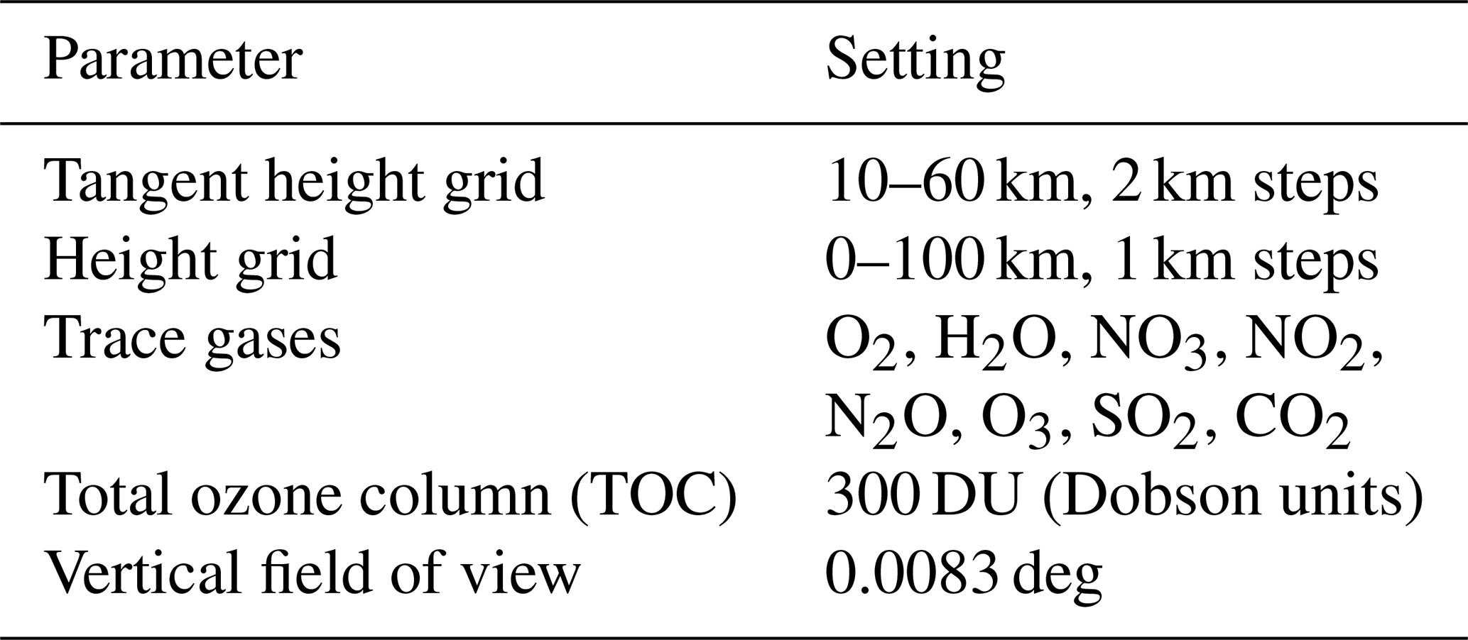
The input parameters, including the viewing geometry, are configured to represent an idealized satellite solar occultation instrument similar to SAGE III/ISS, assuming a satellite altitude of 400 km. The SCIATRAN simulations yield transmission values at 565 nm for tangent heights from 10 to 60 km with a step size of 2 km.

2.2.2 Retrieval

For the stratospheric extinction coefficient profile retrievals, the retrieval algorithm in SCIATRAN version 4.7 was used. The retrieval approach is the regularised inversion with the optimal estimation method. The linearised inverse problem is formulated as follows:

$$\begin{array}{}\text{(1)}& \mathit{y}=F\left({\mathit{x}}_{\mathrm{a}}\right)+\mathbf{K}(\mathit{x}-{\mathit{x}}_{\mathrm{a}})\end{array}$$

with y as measurement vector, containing the logarithms of the transmission values at 565 nm for all tangent heights (no random noise realisations were added to y), F as the radiative transfer operator, x_a the a priori state vector. K is the weighting function matrix and x the state vector (to be retrieved). The approximate solution of the inverse problem is gained by minimising the following expression:

$$\begin{array}{}\text{(2)}& {∥F\left({\mathit{x}}_{\mathrm{a}}\right)+\mathbf{K}(\mathit{x}-{\mathit{x}}_{\mathrm{a}})-\mathit{y}∥}_{{\mathbf{S}}_{\mathit{ϵ}}^{-\mathbf{1}}}^{\mathrm{2}}+{∥(\mathit{x}-{\mathit{x}}_{\mathrm{a}}))∥}_{{\mathbf{S}}_{\mathbf{a}}^{-\mathbf{1}}}^{\mathrm{2}}\end{array}$$

with S_ϵ as the noise covariance matrix and S_a as the a priori covariance matrix. The Gauss-Newton iterative approach is used to formulate the solution for each iteration step x_i+1 as follows:

$$\begin{array}{}\text{(3)}& \begin{array}{rl}{\mathit{x}}_{i+\mathrm{1}}=& {\mathit{x}}_{\mathrm{a}}+{\left({\mathbf{K}}_i^T{\mathbf{S}}_{\mathit{ϵ}}^{-\mathbf{1}}{\mathbf{K}}_i+{\mathbf{S}}_{\mathbf{a}}^{-\mathbf{1}}\right)}^{-\mathrm{1}}\\ & {\mathbf{K}}_i^T{\mathbf{S}}_{\mathit{ϵ}}^{-\mathrm{1}}\left(\mathit{y}-F\left({\mathit{x}}_i\right)+{\mathbf{K}}_i({\mathit{x}}_i-{\mathit{x}}_{\mathrm{a}})\right)\end{array}\end{array}$$

More information on the retrieval algorithm can be found in Rozanov et al. (2011), Sect. 3.4.2.

The relevant input parameters for the extinction coefficient profile retrievals are listed in Table 2. The settings for the tangent height grid, height grid, vertical field of view and total ozone column are the same as for the forward simulations. The defined signal-to-noise-ratio (SNR) varies depending on the tangent height (TH), assuming constant noise:

$$\begin{array}{}\text{(4)}& \mathrm{SNR}\left(\mathrm{TH}\right)={\mathrm{SNR}}_{max}\cdot {\displaystyle \frac{\mathit{T}\left(\mathrm{TH}\right)}{T_{max}}}\end{array}$$

with T_max as the maximum transmission value (≈1 at TH = 60 km), SNR_max as the corresponding maximum SNR (1000 (e.g. Meyer et al., 2005) at TH = 60 km) and T(TH) as the transmission value at the tangent height TH.

Table 2 Relevant input parameters for extinction coefficient profile retrievals.

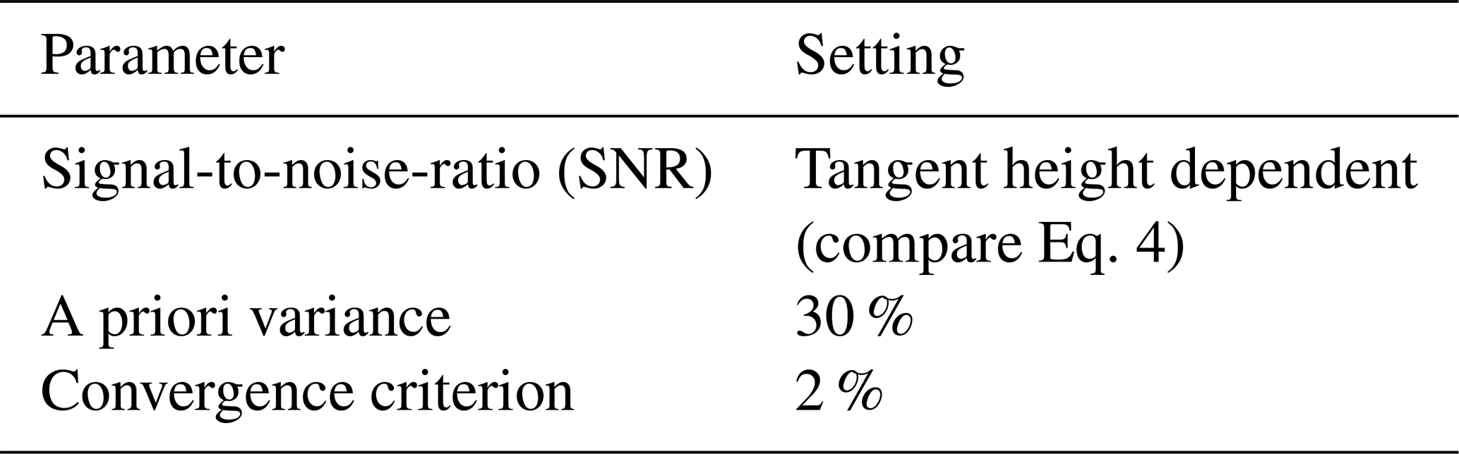
The a priori variance of 30 % allows the retrieval state sufficient freedom to deviate from the a priori and ensures regularisation of the inverse problem, thereby preventing unphysical, oscillating solutions.

The off-diagonal elements of the a priori covariance matrix are defined as follows:

$$\begin{array}{}\text{(5)}& {{\mathbf{S}}_{\mathbf{a}}}^{i,j}={\mathit{\sigma }}^{\mathrm{2}}\exp \left(-{\displaystyle \frac{|z_i-z_j|}{r_{\mathrm{c}}}}\right)\end{array}$$

where σ is the a priori variance, z_i,z_j are the altitudes corresponding to element (i,j) of the covariance matrix, and r_c is the correlation radius, which is set to 3.3 km in this study.

Latitude-dependent background aerosol extinction coefficient profiles (without SAI) at 565 nm from SOCOL-AERv2 simulations were used as a priori information. Output of the retrievals with SCIATRAN are retrieved stratospheric extinction coefficient profiles at 565 nm.

2.3 Error analysis

Under the assumption of random and statistically independent error sources and a linear dependence of the retrieved extinction coefficients on the parameters, the error estimation of the aerosol extinction coefficient was performed as follows:

$$\begin{array}{}\text{(6)}& {\displaystyle }{\displaystyle }{\mathit{\sigma }}_{\text{total}}=\sqrt{\begin{array}{l}{\mathit{\sigma }}_{\text{Noise}}^{\mathrm{2}}+{\mathit{\sigma }}_{\text{Pointing error}}^{\mathrm{2}}+{\mathit{\sigma }}_{\text{Total ozone column}}^{\mathrm{2}}+\\ {\mathit{\sigma }}_{\text{Temperature and pressure}}^{\mathrm{2}}+{\mathit{\sigma }}_{\text{Temperature}}^{\mathrm{2}}+\\ {\mathit{\sigma }}_{\text{Pressure}}^{\mathrm{2}}\end{array}}\end{array}$$

Each term represents individual errors in extinction caused by incorrect knowledge or uncertainties of relevant input parameters, e.g. pressure, temperature, total ozone, and pointing. Note that temperature and pressure are treated as statistically independent error sources, whereas in reality temperature and pressure are physically coupled. This may lead to a slight overestimation of the total error.

The individual errors represent relative differences r (Eq. 7) between the retrieved extinction profiles based on the reference setting and the modified setting (compare Table 3). Here, x_ref,i is the retrieved extinction coefficient at altitude i based on the reference settings and x_i the retrieved extinction coefficient at altitude i based on the modified settings. The noise error was obtained from the noise covariance matrix.

$$\begin{array}{}\text{(7)}& r_i={\displaystyle \frac{x_i-x_{\mathrm{ref},i}}{x_{\mathrm{ref},i}}}\cdot \mathrm{100}\mathit{\%}\end{array}$$

(e.g., Bramstedt et al., 2012)(e.g., Garane et al., 2019)(e.g., Nowlan et al., 2007; Langland et al., 2008)(e.g., Nowlan et al., 2007; Langland et al., 2008)(e.g., Nowlan et al., 2007; Langland et al., 2008)

Table 3 Reference and modified settings for the error analysis.

Based on the methodologies presented here, the following results section uses relevant terminology, which is explained in Table 4.

Table 4 Explanation of the relevant terminology.

3 Results and discussion

Figure 1 shows the order of magnitude as well as the latitude and altitude dependence of the extinction coefficients at 565 nm (1/km) based on the SOCOL-AERv2 simulations for the continuous injection of 5 Tg yr⁻¹ alumina (left panel) and calcite (right panel) in the quasi steady-state phase.

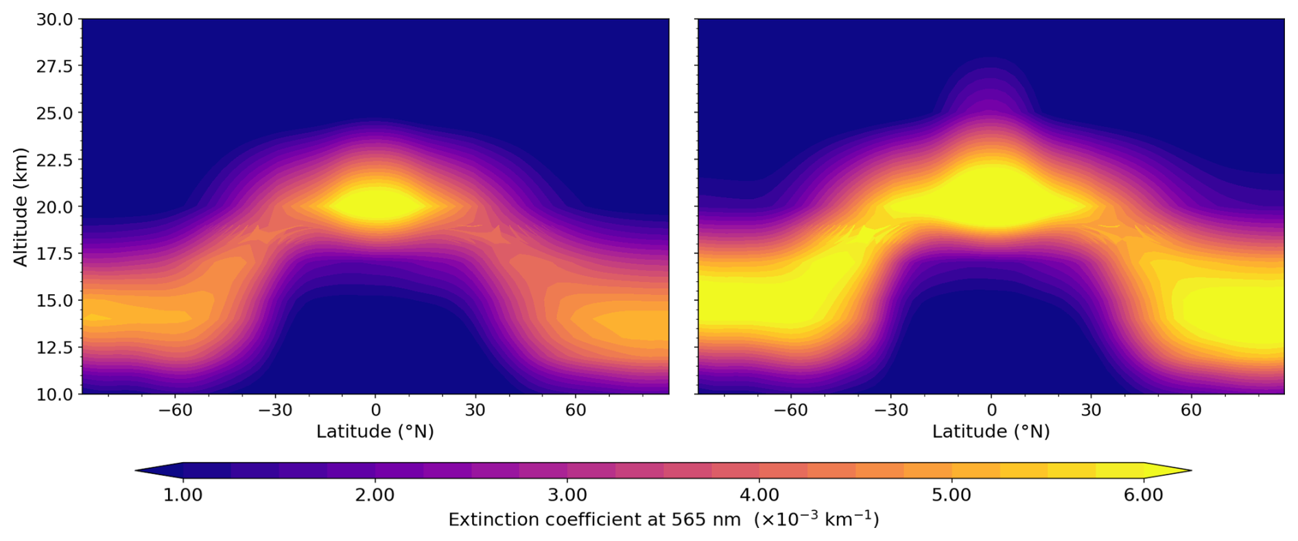
Figure 1 Extinction coefficients at 565 nm based on the SOCOL-AERv2 simulations for the continuous injection of 5 Tg yr⁻¹ alumina (left panel) and calcite (right panel) in the quasi steady-state phase.

Following the approach of Lange et al. (2025), artificial aerosol enhancement is considered detectable if the background profile lies outside the error range of the retrieved extinction coefficient profiles of alumina or calcite. In the following, the detectability of alumina and calcite injections is examined, followed by a discussion of the distinguishability from the natural variability.

3.1 Alumina injection

Figure 2 shows the retrieved extinction coefficient profiles at 565 nm (solid blue lines) for the injection of 5 Tg yr⁻¹ alumina including retrieval uncertainties (in accordance with Eq. 6) (dashed blue lines), background profiles (a priori profiles) (solid purple lines), true profiles (solid orange lines), and tropopause heights (dashed black lines) for (a) 75° N, (b) 75° S, (c) 55° N, (d) 55° S, (e) 35° N, (f) 35° S, (g) 5° N, and (h) 5° S. The tropopause height as well as the background and true profiles are based on the SOCOL-AERv2 model simulations. The results for the different latitudes show that the background profiles lie outside the error range of the retrieved extinction coefficient profiles. For 75° N (panel a), this covers an altitude range from 10 to about 23 km. In contrast, at 75° S (panel b), the background profile (a priori profile) approaches the true profile, and thus also the retrieved profile, at around 20 km and then lies within the error range of the retrieved extinction coefficient profile above this altitude. However, this is not a limitation, as the main altitude range of interest, which also differs from the background, here between 10 and 20 km, lies outside the error range of the retrieved extinction coefficient profile. For latitudes of 55° N (panel c), 55° S (panel d), as well as 35° N (panel e), 35° S (panel f), the background profile lies within an altitude range of approximately 10 to 25 km outside the error range and thus also covers the altitude range relevant for these latitudes. A different pattern is observed at 5° N (panel g) and 5° S (panel h). Here, both the true and retrieved extinction coefficient profiles show a pronounced maximum between approximately 18 and 25 km altitude, where the background profile lies outside the error range of the retrieved extinction coefficient profile. Below this altitude range, the true and retrieved profiles exhibit a steep vertical gradient, i.e. a sharp decrease in the extinction coefficients, before approaching the background profile, which then lies within the error range of the retrieved extinction coefficient profile. This, combined with the difference of around four orders of magnitude at most between the background (a priori) and the true profile, leads to discrepancies between the retrieved and true profiles at lower altitudes (10–13 km). However, as these altitudes fall outside the relevant altitude range for these latitudes, this do not influence the conclusions on detectability.

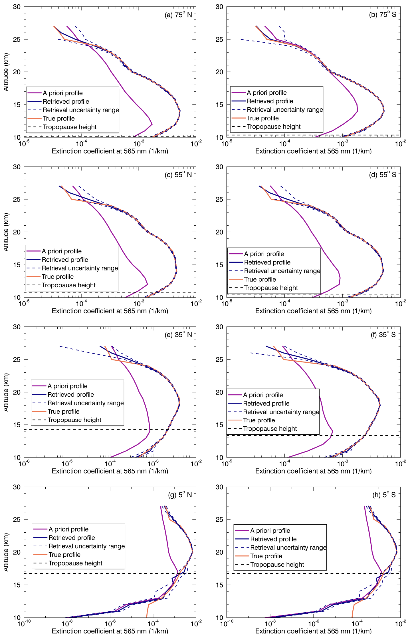
Figure 2 Retrieved extinction coefficient profiles at 565 nm for the injection of 5 Tg yr⁻¹ alumina including retrieval uncertainties, background profiles (a priori profiles), true profiles, and tropopause heights for (a) 75° N, (b) 75° S, (c) 55° N, (d) 55° S, (e) 35° N, (f) 35° S, (g) 5° N, and (h) 5° S.

Considering the assumptions of this study, it can be concluded that the change due to the additional continuous injection of 5 Tg yr⁻¹ of alumina is large enough to be distinguishable from the background and detectable by a typical satellite solar occultation instrument. This suggests that the sensitivity of a typical satellite solar occultation instrument is likely sufficient to detect stratospheric solid particle injections of alumina of the magnitude considered here.

These conclusions are further supported by an analysis of the stratospheric optical depth. Figure 3 illustrates the true (orange line) and background (purple line) stratospheric optical depth at 565 nm based on the SOCOL-AERv2 model simulations. The retrieved stratospheric optical depth including the retrieval uncertainties are depicted as solid and dashed blue lines. The retrieval uncertainties for the retrieved stratospheric optical depth were calculated using Gaussian error propagation. For the calculation of the corresponding optical depth, the latitude-dependent tropopause heights from SAGE II data (2000–2004) were used, which is why only a latitude range of 55° S to 55° N can be shown (NASA, 2012). The tropopause heights from SAGE II were chosen to ensure consistency with the following discussion on the natural variability, which is likewise based on the SAGE II data. The stratospheric optical depth is obtained by integrating the extinction coefficient from the tropopause up to 27 km, consistent with the upper limit of the SOCOL-AERv2 data (see Sect. 2.1).

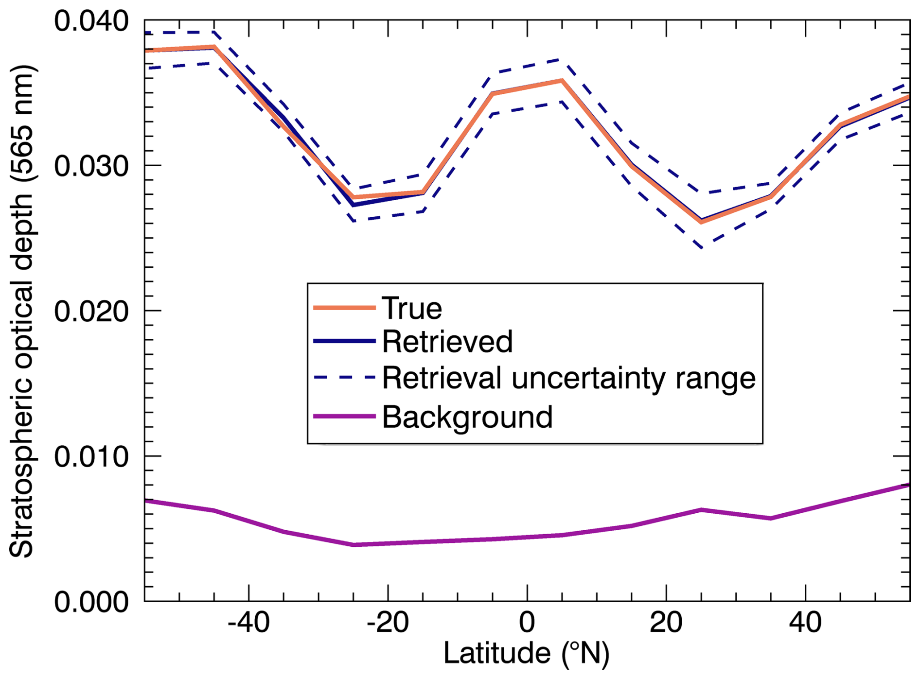
Figure 3 Stratospheric optical depth (565 nm) as a function of latitude for the injection of 5 Tg yr⁻¹ alumina: retrieved (blue line), background (purple line) and true (orange line). The retrieval uncertainties are shown by the blue dashed lines.

The variation in stratospheric optical depth as a function of latitude shows maxima around the Equator and in the mid- and high latitudes, as well as minima in the subtropics. The equatorial maximum results from the continuous injection of 5 Tg yr⁻¹ of alumina in this region (between 30° N and 30° S). The subtropical minima and the maxima at mid- and high latitudes reflect the latitudinal variation of the tropopause height, which decreases from the tropics toward higher latitudes. As the background consistently falls outside the error range of the retrieved profiles across latitudes, the continuous injection of 5 Tg yr⁻¹ of alumina can be considered detectable for the latitudes examined here.

The comparatively high background SAOD in the SOCOL-AERv2 simulations is consistent with findings by Brodowsky et al. (2024). The inter-model spread is attributed in part to differences in OH availability, which controls the rate of oxidation of sulphur dioxide to sulphuric acid in the lower stratosphere, as well as to differences in representation of stratospheric transport (Brodowsky et al., 2024).

It should be noted that the SOCOL-AERv2 model simulations with alumina (and calcite) were performed on the basis of current knowledge and the most reasonable assumptions for, e.g., heterogeneous reaction rates on these injected solid materials (Vattioni et al., 2025). These assumptions and their associated uncertainties should therefore be taken into account when interpreting the results presented here. For more details we refer to Vattioni et al. (2025). Furthermore, the influence of natural variability has not yet been taken into account and will be discussed below.

Consistent with expectations, the retrieval uncertainties, i.e., the total errors shown in Fig. 4, for the retrieval of the stratospheric extinction coefficient profiles for an injection of 5 Tg yr⁻¹ of alumina show a dependence on latitude and altitude. The determination of the total errors is based on the error analysis as described in Sect. 2.3. The high levels of total errors at low and high altitudes arise from the low extinction coefficients and the correspondingly weak signal in this range of altitudes and latitudes. The total error at the injection altitude, in this case 50 hPa (≈20 km), varies between 3 % and 7 %, depending on the latitude.

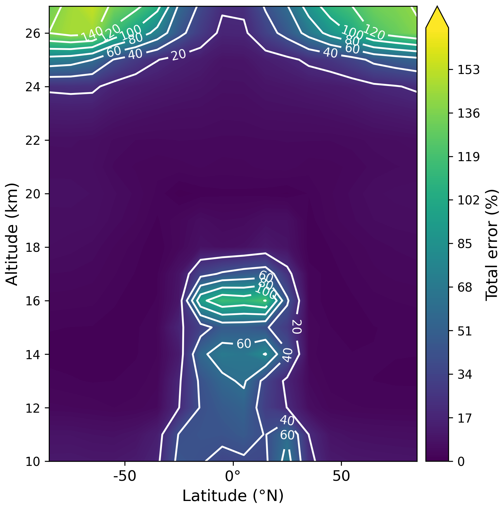
Figure 4 Total error (%) for the retrieval of the stratospheric extinction coefficient profiles for the injection of 5 Tg yr⁻¹ alumina.

3.2 Calcite injection

Figure 5 shows the retrieved extinction coefficient profiles at 565 nm (solid blue lines) for the injection of 5 Tg yr⁻¹ calcite including retrieval uncertainties (in accordance with Eq. 6) (dashed blue lines), background profiles (a priori profiles) (solid purple lines), true profiles (solid orange lines), and tropopause heights (dashed black lines) for (a) 75° N, (b) 75° S, (c) 55° N, (d) 55° S, (e) 35° N, (f) 35° S, (g) 5° N, and (h) 5° S. The tropopause heights as well as the background and true profiles are based on the SOCOL-AERv2 model simulations. Compared with the extinction coefficient profiles based on the injection of alumina (compare Fig. 2), the extinction coefficients for calcite are slightly higher, but still of the same order of magnitude. Consequently, the corresponding profiles deviate more distinctly from the background profiles. In particular, at 75° S (panel b), this leads to detectable signals above ≈20 km (here up to 24 km), where the background profile lies outside the error range of the retrieved profile. For the latitudes of 55° N (panel c) and 55° S (panel d) as well as 35° N (panel e) and 35° S (panel f), the detectable altitude range is similar to that for the alumina injection, ranging from 10 to ≈25 km. The latitudes near the equator (5° N (panel g)/° S (panel h)) also exhibit behaviour similar to that observed in the case of alumina injection. However, for the relevant altitude range of approximately 18 to 27 km, the background profiles lie outside the error range, which supports the conclusion that detection is possible in this altitude range. In summary, it can be concluded that, under the assumptions made, the continuous injection of 5 Tg yr⁻¹ of calcite can very likely be detected with a satellite solar occultation instrument at the altitudes and latitudes considered here.

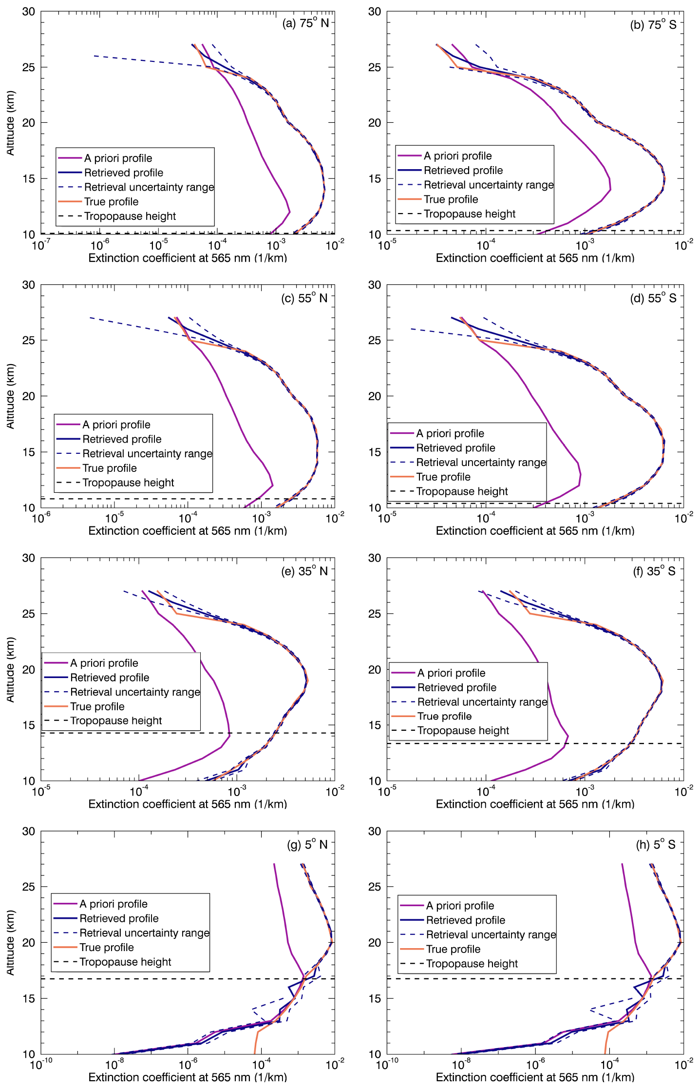
Figure 5 Retrieved extinction coefficient profiles at 565 nm for the injection of 5 Tg yr⁻¹ calcite including retrieval uncertainties, background profiles (a priori profiles), true profiles, and tropopause heights for (a) 75° N, (b) 75° S, (c) 55° N, (d) 55° S, (e) 35° N, (f) 35° S, (g) 5° N, and (h) 5° S.

Analogous to Fig. 3 for alumina injection, Fig. 6 shows the stratospheric optical depth (565 nm) as a function of latitude for the true (orange line), background (purple line), and retrieved (solid blue line) cases, including the retrieval uncertainties (dashed blue line), for the injection of 5 Tg yr⁻¹ calcite. The first two are based on the SOCOL-AERv2 model simulations. The latitudinally dependent tropopause height is here also consistently reflected in the variation of stratospheric optical depth across latitudes, with the maximum occurring in the equatorial region, as this is where the injection takes place (between 30° N and 30° S). Consistent with the methodology for the alumina injection calculations, the latitude-dependent tropopause heights from SAGE II data were used for the calculation of the stratospheric optical depth.

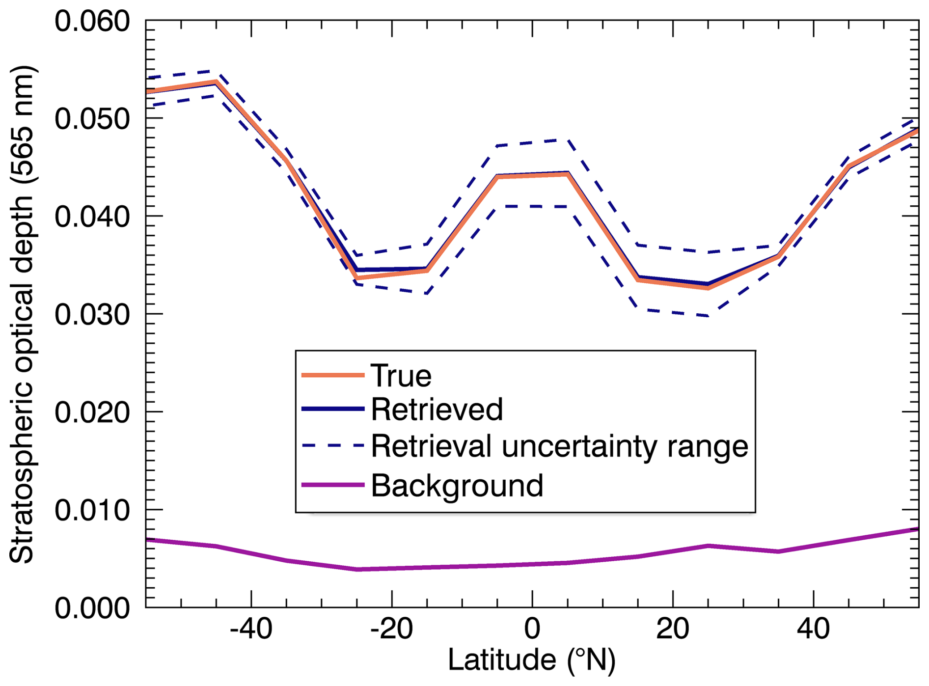
Figure 6 Stratospheric optical depth (565 nm) as a function of latitude for the injection of 5 Tg yr⁻¹ calcite: retrieved (blue line), background (purple line) and true (orange line). The retrieval uncertainties are shown by the blue dashed lines.

The most notable difference between the two scenarios is the magnitude of the stratospheric optical depth. The alumina injection scenario (Fig. 3) yields peak values of approximately 0.036, whereas the calcite injection (Fig. 6) reaches values of around 0.044 at the equatorial maximum. In both cases, the background stratospheric optical depth remains below 0.010 over all latitudes, and the retrieval uncertainty range is comparable in relative magnitude between the two scenarios. As in the alumina case, the background consistently lies outside the error range of the retrieved profiles over all examined latitudes, indicating that the continuous injection of 5 Tg yr⁻¹ of calcite is likewise detectable with a satellite solar occultation instrument. It should be noted that the SOCOL-AERv2 model simulations for calcite are equally based on current knowledge and the most reasonable assumptions for heterogeneous reaction rates on the injected solid material (Vattioni et al., 2025), and the associated uncertainties should be considered when interpreting these results. The natural variability is examined and discussed in Sect. 3.3.

Figure 7 shows the corresponding retrieval uncertainties, i.e., the total errors (Eq. 6), for the stratospheric extinction coefficient retrievals for the injection of 5 Tg yr⁻¹ of calcite. The total errors of the retrieval show a broadly similar spatial structure to those of the alumina case. Elevated total errors exceeding ≈20 % are here also found at altitudes above 24 km at high latitudes, and in the equatorial lower stratosphere around 10–17 km. Both can be attributed to the comparatively low extinction coefficients and the resulting low signals. The total error at the injection altitude (≈20 km) varies between 2 %–4 %, depending on the latitude.

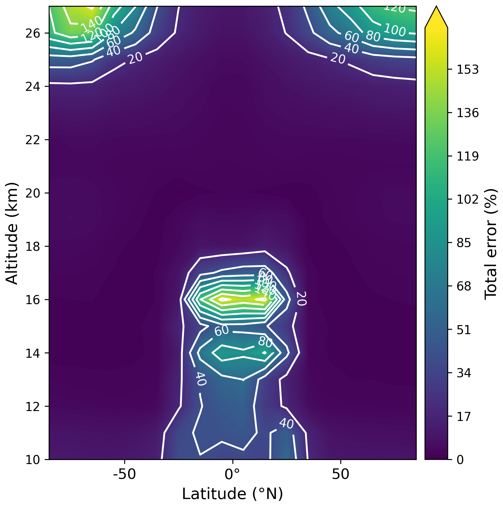
Figure 7 Total error (%) for the retrieval of the stratospheric extinction coefficient profiles for the injection of 5 Tg yr⁻¹ calcite.

The estimated retrieval uncertainties at the injection altitude of ≈20 km (3 %–7 % for alumina and 2 %–4 % for calcite) are comparable to the uncertainties reported for the SAGE III/ISS Level 2 solar aerosol product. Wrana et al. (2021) reported an extinction measurement uncertainty of 5.66 % at 20 km altitude for 520 nm, averaged over June 2017–December 2019.

3.3 Natural variability

The natural variability of the stratospheric optical depth under near-background conditions was evaluated using SAGE II data from 2000–2004 (NASA, 2012). Near-background conditions were chosen, as this represents the most conservative case for detectability. A background disturbed by volcanic activity, for example, would very likely require an SAI strategy adapted to the volcanic eruption, which would mean that the background and the signal would no longer be clearly distinguishable and a separate analysis would be required.

The SAGE II data provides aerosol extinction coefficients at 525 and 1020 nm. To derive the stratospheric aerosol optical depth (SAOD) at 565 nm, as required for comparison, the Ångström exponent interpolation method was applied. The SAOD at 565 nm was calculated considering the latitude-dependent tropopause height. Figure 8 shows the mean SAOD at 565 nm as a function of latitude. The vertical bars indicate the standard deviation of the SAOD values for each latitude of five annual means. It should be noted that the use of the Ångström exponent for wavelength interpolation between 525 and 1020 nm introduces a certain systematic negative bias, as the aerosol extinction spectrum does not strictly follow the assumed power-law relationship (Damadeo et al., 2024). This bias is on the order of a few percent under background aerosol conditions and increases with aerosol loading. However, since the same interpolation method is applied consistently across all latitude bands and years of the reference period, the bias is systematic rather than random and does not affect the relative structure of the natural variability estimate. For the aim of establishing near-background variability bounds, this approach is therefore considered sufficient.

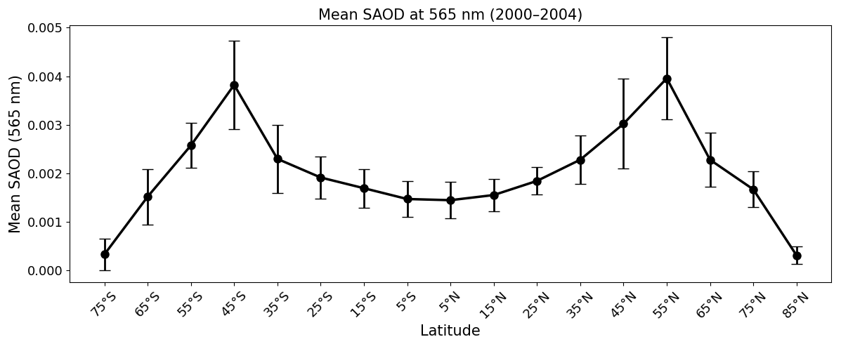
Figure 8 Mean SAOD (565 nm) as a function of latitude for the SAGE II data from 2000–2004. The vertical bars indicate the standard deviation of the SAOD values for each latitude.

The SAI signal of the alumina and calcite injections is considered detectable if the corresponding stratospheric optical depth is outside the 2σ range of the natural variability. For both injection scenarios (compare Figs. 3, 6) this is the case. It can therefore be concluded that the continuous injection of 5 Tg yr⁻¹ of alumina and calcite can also be detected taking into account a realistic measure of the natural variability under near-background conditions. This distinguishability is important because it implies that the injection-induced signal could be attributed to the injections rather than to internal variability, making observational detection of the SAI perturbation in principle feasible.

When interpreting the results presented here, the underlying assumptions must be taken into account. It is not the aim of this study to make general statements about the detection capabilities of all satellite solar occultation instruments, but rather to assess the detectability of SAI scenarios based on solid particles within a consistent simulation framework based on typical satellite solar occultation measurements. And although the latitudinal range examined here is greater than, for example, that covered by SAGE III/ISS, the high latitudes were analysed in order to obtain information on detectability covering as wide a latitudinal range as possible.

It is worth noting that at significantly higher injection rates than the 5 Tg yr⁻¹ considered here, the zero-transmission problem, i.e. very low transmissions from the perspective of the satellite solar occultation instrument, could become relevant for solar occultation retrievals, potentially limiting the detectable range of SAI scenarios (Lange et al., 2026). Within the injection rates examined in this study, however, this effect is not expected to play a role.

4 Conclusions

In this study, SOCOL-AERv2 simulations combined with SCIATRAN radiative transfer calculations were used to investigate whether continuous injections of solid particles into the stratosphere can be detected with typical satellite solar occultation instruments. Two potential SAI materials, alumina and calcite, were considered for an injection rate of 5 Tg yr⁻¹. The results show that the simulated extinction coefficient profiles and corresponding stratospheric optical depths at 565 nm produce clear perturbations relative to the background. For both alumina and calcite, the retrieved extinction profiles differ significantly from the background profiles over relevant altitude ranges and latitudes, even when measurement uncertainties are taken into account. The analysis of the stratospheric optical depth further demonstrates that the simulated SAI signals exceed the 2σ range of natural variability derived from SAGE II observations under near-background conditions. This indicates that the signal caused by continuous injections of 5 Tg yr⁻¹ of alumina or calcite could also be distinguished from natural variability. Accordingly, higher injection rates are also expected to be detectable as an SAI signal and distinguishable from natural variability for near-background conditions.