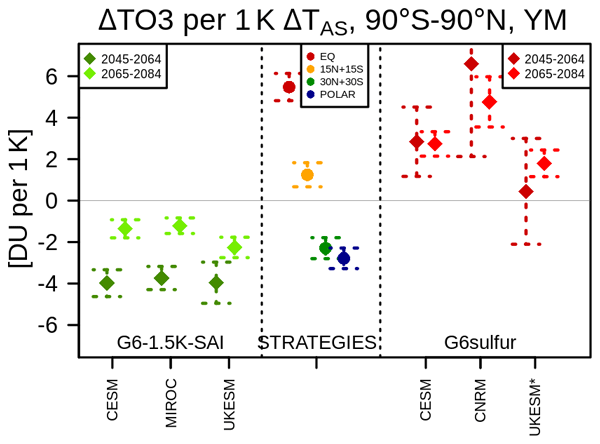
Stratospheric ozone projections under sulfur-based stratospheric aerosol injection: Insights from the multi-model G6-1.5K-SAI experiment

Owing to the crucial role of stratospheric ozone in shielding the Earth from harmful solar ultraviolet radiation, impacts of human activities on the ozone layer remain of interest. Here we provide an assessment of the potential impacts of Stratospheric Aerosol Injection (SAI), a proposed method to temporarily offset global warming, on stratospheric ozone projections over the 21st century using the new multi-model GeoMIP G6-1.5K-SAI experiment. The experiment injects SO₂ at a pair of subtropical latitudes and utilizes a more plausible “middle-of-the-road” greenhouse gas emission pathway (SSP2-4.5) and SAI start date compared to earlier studies.

All three participating Earth system models show a decrease in global mean total column ozone of a few Dobson units (1 %–2 %) under SAI compared to the no-SAI scenario. This decrease is dominated by enhancement in active halogens from heterogenous chemistry on sulfate aerosol, most clearly evident in the Southern Hemisphere mid- and high latitudes. This is unlike previous results using strategies injecting at the equator, which show increased global mean column ozone, partly due to larger ozone transport changes. As background halogen levels continue to decrease, the potential of SAI to deplete ozone is found to be a factor of ∼ 2 larger in earlier part of the 21st century (2045–2064) than later (2065–2084). We further identify areas of model disagreement and sources of uncertainty, but also areas of more confidence and potential emergent constraints. Our results highlight the need to assess any projected SAI impacts in the wider strategy and scenario dimension using a multi-model framework.

1 Introduction

Stratospheric ozone plays a crucial role in life and ecosystems on Earth, shielding the surface from harmful ultraviolet solar radiation. Since the discovery of the ozone hole by Farman et al. (1985), international research has focused extensively on how human activities – especially emissions of both long- and short- lived ozone depleting substances (ODSs) and greenhouse gases (GHGs) – can drive significant changes in this important atmospheric constituent (World Meteorological Organization, 2022). More recently, such research has expanded to include impacts from so-called “climate intervention” or “geoengineering” methods, the proposed methods aiming to temporarily offset some of the most negative impacts of climate change. The most extensively studied method, termed Stratospheric Aerosol Injection (SAI), involves introducing reflective aerosols (typically sulfate), or their precursors, into the lower stratosphere in order to reduce solar radiation reaching the troposphere, in a manner analogous to that occurring under explosive sulfur-rich volcanic eruptions.

SAI can affect stratospheric ozone via a range of chemical and dynamical processes (e.g. Pitari, et al., 2014; Haywood and Tilmes, 2022; Bednarz et al., 2023a, b). Amongst other factors, sulfate aerosols provide active surfaces that facilitate heterogeneous halogen and nitrogen reactions that impact concentrations of species directly relevant for chemical ozone production and loss. Furthermore, sulfate aerosols absorb some of the incoming solar and outgoing terrestrial radiation, thereby warming the lower stratosphere where they reside. The resulting temperature changes alter atmospheric circulation and affect ozone transport. Any resulting local changes in temperature can further modulate stratospheric chemistry, whether by altering the rates of gas-phase and heterogeneous chemical reactions, impacting formation of polar stratospheric clouds, or modulating stratospheric water vapor content by warming the cold-point tropical tropopause.

Given the range of processes affecting stratospheric ozone, all of which can be uniquely affected by different SAI realizations, the analysis of ozone response to SAI needs to account for details of SAI strategy and scenario used, as well as potential sources of inter-model differences. However, to date research exploring the above aspects has been relatively limited. Using a single model, the Community Earth System Model (CESM), SAI impacts on ozone have been studied with a focus on the choice of SAI strategy (i.e. location of injection; Bednarz et al., 2023a; Tilmes et al., 2021), magnitude of surface cooling (Bednarz et al., 2023b), underlying GHG emission scenario (Tilmes et al., 2020; Haywood and Tilmes, 2022) and the start date of SAI (Brody et al., 2024). However, studies exploring these aspects consistently across different models are scarce or incomplete. For example, Henry et al. (2024) used UKESM to explore the role of SAI strategy on ozone, but their model version lacked coupling of heterogeneous chemical reactions and sulfate aerosols from SAI, thereby missing an essential process that could affect ozone. Most recently, Jörimann et al. (2026) used a multi-model ensemble of SAI simulations participating in the ongoing phase 2 of the Chemistry Climate Model Intercomparison project (CCMI-2022; Plummer et al., 2021). While providing invaluable insights on the models' sensitivities to imposed stratospheric sulfate aerosols in an atmosphere-only set-up, the experiment, by design, excluded some important sources of uncertainty driving the aerosol, climate and ozone responses to the intervention.

Most other multi-model studies assessing SAI impacts on ozone come from the previous simulations from the Geoengineering Model Intercomparison Project (GeoMIP), in particular the “G6sulfur” experiment with SO₂ (the gaseous precursor to sulfate aerosol) injection in the equatorial lower stratosphere (Kravitz et al., 2015). Three models with interactive chemistry participated in that experiment, and the resulting stratospheric ozone responses were discussed in Tilmes et al. (2022) and Haywood and Tilmes (2022). It has since been shown that SAI in the equatorial region leads to many undesirable side effects and poorer skill and efficiency in reaching chosen climate objectives compared to strategies injecting SO₂ in the off-equatorial or subtropical regions (e.g. Kravitz et al., 2019; Zhang et al., 2024; Bednarz et al., 2023a; Wells et al., 2024; Henry et al., 2024). Hence, a new GeoMIP experiment – named G6-1.5K-SAI – has been proposed that addresses some of those shortcomings by injecting SO₂ at a pair of subtropical (30° N and 30° S) latitudes symmetrically around the equator (Visioni et al., 2024; Lee et al., 2026). This experiment aims to be more policy relevant than the older G6sulfur by using the “middle-of-the-road” Shared Socioeconomic Pathway (SSP) SSP2-4.5 GHG scenario (Meinshausen et al., 2020), which is closer to current climate policies and commitments than the “business-as-usual” SSP5-8.5 GHG scenario used in G6sulfur. It also enables direct comparison with future CMIP7 simulations with similar underlying emission scenarios.

In this paper we utilize the results of this new G6-1.5K-SAI experiment to provide an updated multi-model comparison of SAI impacts on stratospheric ozone and its projections over the 21st century. We also compare some of these results with the previous CESM simulations exploring the role of SAI strategy in Bednarz et al. (2023a). We do this to understand how the choice of different SAI strategy (in particular injection at 30° N and 30° S here compared to injection at the equator in G6sulfur) affects the simulated ozone responses, and also to understand the relative importance of model structural uncertainties compared to the uncertainties coming from the choice of SAI strategy within a single model. The remainder of the paper is structured as follows. Section 2 gives an overview of the G6-1.5K-SAI experiment and the models used. Section 3 discusses the evolution of global mean total column ozone in the simulations. We then focus on changes in tropical (Sect. 4), mid-latitude (Sect. 5) and springtime polar (Sect. 6) ozone, including an assessment and a discussion of drivers of the diagnosed responses. Section 7 explores the role of heterogeneous chemical processes versus transport changes for the SAI ozone response using a set of sensitivity experiments with the UKESM model. Finally, Section 8 summarizes and discusses the main results.

2 Methods

We use the new GeoMIP G6-1.5K-SAI simulations proposed in Visioni et al. (2024), which result in aerosol burdens and large scale surface climate responses shown in Lee et al. (2026). Briefly, the simulations follow the CMIP6 SSP2-4.5 GHG emission scenario. The SAI simulation aims to mitigate the global mean temperature increase occurring in SSP2-4.5 (Fig. 1a) by including a symmetrical SO₂ injection in the lower stratosphere at ∼ 21 km altitude at two gridboxes closest to 30° S and 30° N in latitude. The SO₂ injection starts in 2035 and continues until 2084, with the magnitude of the injection (Fig. 1b) adjusted interactively in each model at the beginning of a year in order to maintain global mean near-surface air temperatures at the baseline level, taken as the ensemble mean 2020–2039 average of each of the model's SSP2-4.5 ensemble (Fig. 1a).

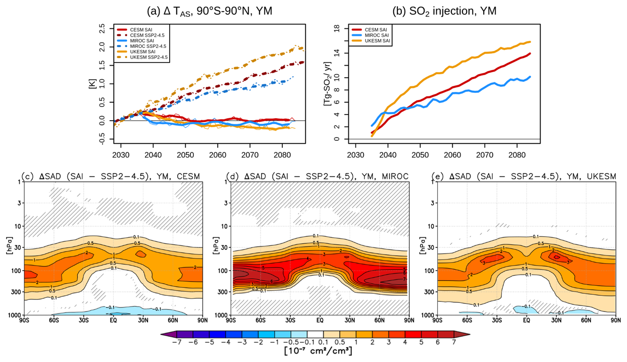
Figure 1 Top: (a) Timeseries of ensemble mean changes in annual mean (“YM”) global mean near-surface air temperature (T_AS) in each model (colors) in the G6-1.5K-SAI (solid) or SSP2-4.5 experiments (dashed). Anomalies are calculated relative to each model's baseline (i.e. 2020–2039 ensemble mean of the SSP2-4.5 simulation). Thin lines denote the ensemble mean changes and thick lines denote their 5-year running means. (b) Timeseries of ensemble mean annual SO₂ injection rates in each model's G6-1.5K-SAI experiment (colors). Bottom: (c–e) Annual 2045–2064 mean changes in aerosol surface area density (SAD) between G6-1.5K-SAI and SSP2-4.5 over the same period in each model (columns). Hatching marks the region where the response is not statistically significant (taken as smaller than ±2 standard errors in the difference in means, calculated using standard deviations of both SAI and no-SAI experiments with 20 annual mean values per ensemble members).

There are 3 Earth system models used in this study: the Community Earth System Model version 2.1 coupled to the Whole Atmosphere Community Climate Model version 6, CESM2(WACCM6) (Danabasoglu et al., 2020; hereafter referred to as “CESM”); the Model for Interdisciplinary Research on Climate, MIROC-ES2H (Kawamiya et al., 2020; hereafter referred to as “MIROC”); and the UK Earth System Model version 1.1, UKESM1.1 (Mulcahy et al., 2023; hereafter referred to as “UKESM”). These models are described in more detail in Lee et al. (2026). Regarding model aspects more relevant for the simulated ozone response, Table S1 (supplement) lists heterogeneous chemical reactions occurring on stratospheric sulfate aerosols in each model. All models include a number of most important heterogeneous chlorine, bromine and nitrogen reactions, with MIROC including the most comprehensive list of reactions. We also note that while all three models include interactive photolysis schemes that account for changes in solar zenith angle and overhead ozone column, MIROC and UKESM further include interactive coupling of stratospheric sulfate aerosols and photolysis rates while CESM does not. Regarding the number of ensemble members, CESM performed 3 ensemble members of the G6-1.5K-SAI simulation and 5 ensemble members of the SSP2-4.5 simulation, MIROC performed 10 ensemble members of both the G6-1.5K-SAI and SSP2-4.5 simulations, and UKESM performed 3 ensemble members of both the G6-1.5K-SAI and SSP2-4.5 simulations. The analysis of intra-ensemble variability in the simulated global mean near-surface temperatures, including differences in baseline temperature targets, is found in Lee et al. (2026).

Table 1 Differences between the ensemble mean G6-1.5K-SAI and SSP2-4.5 simulations in the global mean near-surface air temperature, annual SO₂ injection rate, and global mean near-surface air temperature change per 1 Tg-SO₂ yr⁻¹ injection rate, averaged over either the 2045–2064 or 2065–2084 periods.

Importantly, the default G6-1.5K-SAI UKESM simulations (as presented in Lee et al., 2026) do not include heterogeneous chemistry on sulfate aerosols produced by the microphysical model from the SAI SO₂injection (this caveat also applies in the studies of Tilmes et al., 2022; Henry et al., 2024). In those simulations heterogenous reactions can only occur on the background imposed CMIP6-recommended stratospheric aerosol surface area density (SAD) field (used to account for climatological background from potential future volcanic eruptions). Since heterogeneous reactions on SAI sulfate constitute a crucial pathway by which SAI could affect stratospheric ozone, in this study a second revised set of both SSP2-4.5 and G6-1.5K-SAI simulations was carried out with UKESM that include heterogeneous chemical reactions on SAI sulfate. Notably, doing so required switching off heterogenous reactions on the background imposed SAD field; this results in slightly higher climatological global mean ozone column (Fig. S1a, supplement) and, hence, slightly higher global mean near-surface temperature (Fig. S1b) in the revised UKESM SSP2-4.5 compared to the original experiment (Fig. S1b). This also affects our revised UKESM G6-1.5K-SAI because the same absolute near-surface temperature target from the original SSP2-4.5 was used, leading to a slight overcooling (∼ 0.2 K) compared to the reference (2020–2039 mean surface temperature in the revised SSP2-4.5, Fig. 1a). We note this slight overcooling occurs under smaller SO₂ injection rates (Fig. S1c), as the SAI-induced ozone reduction (Sect. 3) acts to amplify the aerosol-induced surface cooling. Correspondingly, the estimated cooling values per 1 Tg-SO₂ yr⁻¹ injected shown for UKESM in Table 1 are about 0.01 K per Tg-SO₂ yr⁻¹ higher than in the original simulations discussed in Lee et al. (2026). Nonetheless, we expect this overcooling to have only a marginal impact on stratospheric ozone, especially when analyzing the differences between the SAI and no-SAI simulations, the effect of which is expected to be by far offset by the effect of including heterogeneous chemistry on SAI sulfate. In addition, we present many of the results as values normalized with the magnitude of the associated global mean near-surface SAI-induced cooling, hence further removing effects from small inconsistencies in the temperature target definitions. Finally, since the background SAD is not included in either SSP2-4.5 and SAI simulations, we assume the impact of this on ozone is the same in both simulations and thus cancels out when inferring the ozone response to SAI in the model (calculated as the difference between G6-1.5K-SAI and SSP2-4.5). However, this might not necessarily be the case if the chemical ozone response is significantly non-linear to increasing SAD magnitudes. If so, the impact removing such background SAD would have on ozone may be larger in the SSP2-4.5 simulation than in the SAI simulation (where SAI SAD ≫ background SAD), thus potentially increasing the inferred chemical ozone response to SAI in the model.

The analysis of sulfate burdens and aerosol optical depths is discussed in Lee et al. (2026). Here we focus only on the resulting changes in aerosol SAD, the variable most relevant for heterogeneous chemistry and the resulting ozone impacts. As shown in Fig. 1c–e, the three models disagree regarding the projected SAD changes. Comparing CESM and UKESM, CESM shows smaller SAD values in the subtropics and mid-latitudes than UKESM, likely the result of a much faster climatological shallow branch of the Brewer Dobson Circulation (BDC) in CESM that more quickly transports aerosols away from their injection latitude (Bednarz et al., 2023c). In the polar regions, UKESM has higher SAD than CESM in the Arctic stratosphere but lower SAD than CESM in the Antarctic. In MIROC, the simulated SAD is significantly higher (a factor of ∼ 2) than in UKESM and CESM, despite MIROC showing the smallest amount of global warming under SSP2-4.5 needed to be offset with SAI and hence the smallest SO₂ injection rates (Fig. 1a–b). This could be partly related to the lack of coarse aerosol mode in MIROC (Sekiya et al., 2016), resulting in most of SAI aerosol present in the accumulation mode which has lower radius (hence larger surface area) and longer lifetime. Much higher SAD values were also previously found in MIROC simulations of impacts from the 2022 Hunga volcanic eruption (Bednarz et al., 2026), albeit the associated chemical ozone loss in the model was found to be nonetheless comparable to that in other models in that study with much smaller SAD, highlighting that the uncertainty in SAD change is just one of many sources of uncertainty in the resulting ozone response to SAI.

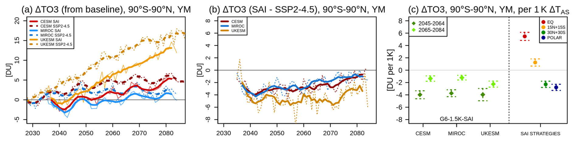
Figure 2 Annual and global mean total column ozone (TO3) changes for each of the models. (a) Timeseries of differences from the baseline period (2020-2039 mean of SSP2-4.5) in the control SSP2-4.5 simulations (dashed) and the corresponding G6-1.5K-SAI simulations (solid). (b) Timeseries of differences between the G6-1.5K-SAI and SSP2-4.5 simulations. Thin lines in (a)–(b) denote the ensemble mean changes for each model and thick lines denote their 5-year running means. (c) Normalized total column ozone changes between the G6-1.5K-SAI and SSP2-4.5 simulations averaged over either 2045–2064 or 2065–2084 periods and scaled with the corresponding global mean near-surface air temperature change. Shown also are the corresponding changes (2050–2069) in the different SAI strategies with CESM2(WACCM6-MA) – EQ, 15N + 15S, 30N + 30S, POLAR – discussed in Bednarz et al. (2023a), see text for more detail. The error bars represent ±2 standard errors in the difference in means, calculated from the annual mean values (20 per ensemble member).

3 Global mean ozone

Figure 2 shows the evolution of global mean total column ozone. In all the SSP2-4.5 simulations (dashed lines in Fig. 2a), global mean total column ozone is projected to increase over the 21st century. This is the combined result of the ongoing reductions in stratospheric halogen concentrations achieved by the Montreal Protocol and its subsequent Amendments and Adjustments, as well as stratospheric cooling and an accelerated BDC as the result of increasing GHG emissions (World Meteorological Organization, 2022). Nonetheless, there are large differences in the magnitude of this ozone increase amongst the different models, with UKESM showing the largest increase (approx. +16 DU global mean total column ozone increase by 2080) and MIROC the smallest (approx. +2 DU increase by 2080). As shown in Fig. S2a–c, while models generally agree on the magnitude of upper stratospheric ozone increase, there are large differences amongst the models in the magnitude of the response in the lower stratosphere, i.e. where ozone concentrations are not just controlled by chemical changes but are also strongly driven by changes in circulation and transport (e.g. World Meteorological Organization, 2022). The inter-model differences in the magnitude of the projected total column ozone increase are qualitatively consistent with the associated differences in the GHG-induced global warming, with UKESM showing the largest concurrent global mean near-surface temperature increase and MIROC the smallest (Fig. 1a).

Once SAI is started in 2035, global mean total ozone columns decrease within a few years compared to the respective SSP2-4.5 simulations, and remain lower throughout the length of the simulations (Fig. 2a–b). The relative ozone reductions are in the order of 1 %–2 % of the 2020–2039 baseline levels, and tend to be larger earlier in the century than later in the century. The latter occurs despite the increasing SO₂ injection rates (and hence increasing stratospheric aerosol burden) over the course of the 21st century in order to offset progressively higher surface temperatures under rising GHGs (Fig. 1a–b). This arises because the reduction in global mean ozone levels under SAI in G6-1.5K-SAI is dominated by the halogen-catalyzed ozone loss in the lower stratosphere facilitated by halogen activation from heterogenous reactions on sulfate aerosols. These increase active halogens either directly via heterogenous halogen reactions (most important at low temperatures in the polar regions) or indirectly via heterogenous N₂O₅ hydrolysis reducing active nitrogen levels and, as the result, increasing active halogens. The extent to which SAI can cause halogen activation and halogen-catalyzed ozone depletion depends on the background stratospheric halogen levels, which are projected to decrease over the course of the 21st century. Hence, for a given amount of SAI this effect is stronger earlier in the century. This is illustrated on the left side of Fig. 2c, whereby the global total column ozone change from SAI is normalized by the associated amount of SAI-induced global mean near-surface air cooling (Table 1). Such approach allows comparison of the impact of SAI aerosol on ozone in the prism of the “intended” aerosol-induced surface cooling, and can thus aid discussion of trade-offs of different SAI choices (scenarios and strategies). In all three models, the decrease in global ozone is a factor of ∼ 2 larger in 2045–2064 (−4 DU K⁻¹) compared to 2065–2084 (−1 to −2 DU K⁻¹), with a relatively good quantitative agreement amongst the models. When normalized with the associated mean SO₂ injection rate (Table 1), we find global mean ozone column losses of −0.4 DU per Tg-SO₂ yr⁻¹ in 2045–2064 and −0.15 to −0.3 DU per Tg-SO₂ yr⁻¹ in 2065–2084.

The G6-1.5K-SAI simulations represent just one SAI strategy with symmetric injection at 30° N and 30° S. However, as shown in Bednarz et al. (2023a), the choice of SAI strategy can play a first order role in determining many of the SAI responses, especially those occurring in, or affected by, changes in the stratosphere. For that reason, in Fig. 2c we compare the G6-1.5K-SAI ozone responses with the corresponding ozone responses diagnosed for the different SAI strategies (over 2050–2069) within a single model discussed in Bednarz et al. (2023a): annual mean injection at 21.5 km altitude at the equator (“EQ”), tropics at 15° N and 15° S (“15N + 15S”) and subtropics at 30° N and 30° S (“30N + 30S”, i.e. the same strategy as in G6-1.5K-SAI) as well as springtime injection at 15 km at 60° N and 60° S (“POLAR”). The simulations followed the same SSP2-4.5 background GHG emission scenario and the model used in that study – CESM2(WACCM6-MA) – was similar to that used in the CESM G6-1.5K-SAI runs, albeit WACCM6-MA has a different chemistry scheme tailored for the middle atmosphere (MA) studies and including only a simplified representation of tropospheric chemistry (Davis et al., 2023). Nevertheless, Davis et al. (2023) showed overall similar climatology and evolution of stratospheric ozone between the two model versions.

Unlike the relatively good multi-model agreement in the normalized global mean total column ozone response to SAI across the G6-1.5K-SAI models, there is a much larger spread in the ozone response to different SAI strategies, ranging from +5.5 DU K⁻¹ for the equatorial strategy to −2.8 DU K⁻¹ in the polar strategy (Fig. 2c). As discussed in Bednarz et al. (2023a), the overall increase in global mean ozone in EQ and 15N + 15S arises from the dominant role of the SAI-induced modulation of the BDC and the associated ozone transport by the residual circulation, alongside reduction in active nitrogen levels in the middle stratosphere (and the resulting nitrogen-catalyzed chemical ozone loss) from heterogeneous N₂O₅ hydrolysis on sulfate. The overall decrease in global mean ozone in 30N + 30S and POLAR in turn arises because of the dominant role of the SAI-induced halogen activation from heterogeneous chemistry on sulfate and halogen-catalyzed chemical ozone loss in the lower stratosphere. For the strategy injecting SO₂ at 30° N and 30° S, the ozone response from the simulations in Bednarz et al. (2023a), diagnosed over 2050–2069, falls in between the range of ozone responses diagnosed from the G6-1.5K-SAI simulations over 2045–2064 and 2065–2084. The results illustrate that, for the global mean ozone response to SAI, the choice of SAI strategy in one model can have a much larger role than inter-model uncertainty. An additional takeaway is that the subtropical strategy used in G6-1.5K-SAI, while potentially having fewer climate side effects than strategies injecting at the equator (as was the case for the earlier G6sulfur experiment; see Lee et al., 2026), leads to a net global mean total column ozone loss. This highlights the trade-offs between optimizing surface climate response and minimizing negative impacts on stratospheric ozone. However, these conclusions are for global mean ozone, while the results differ depending on the region in question, and as such the following sections analyze the corresponding regional ozone responses in more detail.

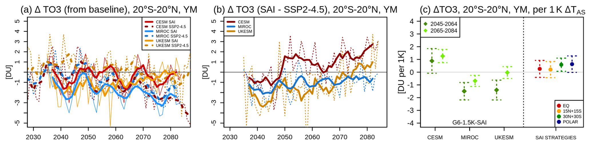
Figure 3 Annual mean tropical (20° S–20° N) total column ozone changes for each of the models. (a) Timeseries of differences from the baseline period (2020–2039 mean of SSP2-4.5) in the control SSP2-4.5 simulations (dashed) and the corresponding G6-1.5K-SAI simulations (solid). (b) Timeseries of differences between the G6-1.5K-SAI and SSP2-4.5 simulations. Thin lines in (a)–(b) denote the ensemble mean changes for each model and thick lines denote their 5-year running means. (c): Normalized total column ozone changes between the G6-1.5K-SAI and SSP2-4.5 simulations averaged over either 2045–2064 or 2065–2084 periods and scaled with the corresponding global mean near-surface air temperature change. Shown also are the corresponding changes (2050–2069) in the different SAI strategies discussed in Bednarz et al. (2023a; see text for more details). The error bars represent ±2 standard errors in the difference in means, calculated from the annual mean values (20 per ensemble member).

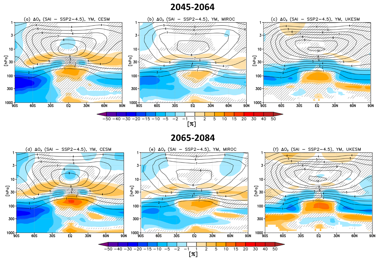
Figure 4 Shading: Annual (top, a–c) 2045–2064 mean and (bottom, d–f) 2065–2084 mean changes in ozone (O₃) volume mixing ratios between the G6-1.5K-SAI simulations and the SSP2-4.5 simulations over the same period for each model (columns). Contours show the corresponding climatological ozone volume mixing ratios (in ppm) in the SSP2-4.5 runs for reference. Hatching marks the region where the response is not statistically significant (defined as in Fig. 1).

4 Tropical ozone

Unlike the projected increase in global mean total column ozone, the tropical ozone column is projected to decrease slightly under the SSP2-4.5 scenario over the second part of the 21st century (Keeble et al., 2021), with differences in the projected trends, including their signs, across different models (Davis et al., 2026; also Fig. 3a for the models used here). This arises because of offsetting between the ozone decrease in the lower stratosphere and ozone increase in the upper stratosphere (Fig. S2a–c). The lower stratospheric ozone reduction arises because of the GHG-induced acceleration of the BDC and the resulting increased transport of ozone-poor tropospheric air into the lower stratosphere; the ozone increase in the upper stratosphere arises due to reduction in chemical ozone loss as halogen levels are reduced and the stratosphere cools (e.g. Keeble et al., 2017; Davis et al., 2026).

For the SAI-induced changes, the models disagree on the sign of the total column ozone response in the tropics (Fig. 3b); while the magnitudes of the column changes are also relatively small (i.e. a few DU) they are comparable to those seen in the SSP2-4.5 simulations with time (Fig. 3a). CESM shows a slight (approx. −1 DU) tropical ozone column decrease compared to SSP2-4.5 over the first decade or so after SAI is started in 2035, followed by a relative ozone increase throughout the rest of the simulation (up to approx. +2–3 DU by early 2080s). MIROC shows a small ozone decrease (up to approx. −2 DU) throughout the simulation that is larger initially and gets smaller with time. UKESM in turn shows the largest ozone decrease (up to approx. −3 DU) compared to SSP2-4.5 in the first decade which then also weakens in magnitude with time and turns into a small net increase in tropical total column by the late 2070s.

These differences in tropical total column ozone responses amongst the three models reflect the complex pattern of tropical ozone changes at different altitudes. As shown in Fig. 4, all three models project relative tropical ozone increases near the tropopause and the lower stratosphere under SAI compared to SSP2-4.5, followed by relative ozone decreases above it at ∼ 40–30 hPa and ozone increases again at ∼ 20–15 hPa. However, there are differences amongst the models regarding the horizontal and vertical extents of these anomalies as well as their magnitudes (and how those change in time). These anomalies of different signs are driven by different processes (see below) and act to offset each other, leading to a relatively uncertain sign and magnitude of the total column response in the tropics (Fig. 3b). We note that this also depends on the exact choice of latitudes that are considered to define the tropics (Fig. S3). Given that climatological total column ozone values are relatively lower in the tropics compared to the rest of the globe and the insolation is higher, relatively small total column ozone changes in this region can still play an important role.

In the tropical lower stratosphere, ozone concentrations are higher under SAI relative to SSP2-4.5 due to the SAI-induced lower stratospheric warming (Figs. 5a–c, 6a) and the resulting deceleration of upwelling in the tropical upper troposphere and lower stratosphere (UTLS) region and shallow branch of the BDC (Fig. 6b; see also Bednarz et al., 2023a; Tilmes et al., 2018). The slowing of the shallow branch of the BDC is also evidenced by the increase in model age-of-air in the lower stratosphere (Fig. 5d–e) and is associated with less transport of ozone poor tropospheric air into the lower stratosphere. Since SAI-induced changes in stratospheric circulation and BDC tend to scale with the magnitude of tropical lower stratospheric warming (Bednarz et al., 2023a, b; Henry et al., 2024), there is a general tendency for models (such as CESM) and strategies (such as the EQ injection) with larger lower stratospheric warming to also show larger changes in stratospheric circulation (Fig. 6). As such, the 30N + 30S strategy used in G6-1.5K-SAI does not lead to as big changes in stratospheric circulation as some previous SAI simulations, e.g. G6sulfur, that inject SO₂ more in the equatorial region.

The relative reduction in tropical ozone under SAI compared to SSP2-4.5 at ∼ 40–30 hPa (Fig. 4) likely results from the acceleration of tropical upwelling above the aerosol layer and the deep branch of the BDC (Bednarz et al., 2023a, b) as well as from the enhanced halogen-catalyzed chemical loss under higher active halogen levels (Fig. 7a–c). This ozone decrease is smallest in CESM, where it was previously found to not be strongly indicative of changes in halogen chemistry (Tilmes et al., 2018, 2021). However, this ozone loss is significantly larger in MIROC and UKESM, as is the concurrent increase in active halogen concentrations in the tropics (as exemplified by ClO changes in Fig. 7a–c). In addition, the corresponding normalized total column response (per 1 K surface cooling; Fig. 3c) in these two models is significantly more negative in the early period (2045-2064) than the later period (2064–2084), suggesting that halogen chemistry does indeed play an important role in contributing to the tropical ozone response in MIROC and UKESM. Above it, the off-equatorial ozone increase at ∼ 20–15 hPa is in turn likely indicative of the reduction in active nitrogen concentrations (as exemplified by the NO₂ changes in Fig. 7d–f) due to enhancement of N₂O₅ hydrolysis on sulfate and the resulting reduction in nitrogen-catalyzed chemical ozone loss at these altitudes.

An additional process that could decrease tropical total column ozone is an acceleration of hydrogen-catalyzed chemical loss under increased stratospheric water vapor brought about by warming of the cold point tropical tropopause (e.g., Tilmes et al., 2018, 2021). However, as shown in Fig. 7g–i, there are substantial differences across the models regarding both the climatological stratospheric water vapor mixing values (contours) as well as the projected stratospheric water vapor changes in response to SAI (shading). The much lower climatological stratospheric water vapor in MIROC (Fig. 7h) might act to reduce relative humidity and hence aerosol water uptake, thus partially contribute to the model showing comparable amount of halogen activation from heterogeneous processing on sulfate, and halogen-catalyzed ozone depletion than the other two models (Sect. 3, also Sects. 5–6) despite much larger aerosol SAD (Sect. 2, Fig. 1d). For the SAI response, CESM simulates tropical water vapor increase of approx. +5 %–10 %, MIROC shows a much smaller water vapor increase of up to approx. +1 %–5 %, and UKESM in fact shows a relative reduction of stratospheric water vapor of up to approx. −10 %. The negative stratospheric water vapor response to SAI in UKESM is associated with much smaller lower stratospheric heating – and thus warming of the cold point tropopause – than the other two models (Fig. 5c), and suggests that processes other than changes in cold point tropopause temperatures could be more important in determining the overall stratospheric water vapor response to the sub-tropical SAI strategy in the model. Such potential factors may include: changes in tropical tropopause pressure, overshooting tropical convection, cross-tropopause transport in the extra-tropical lowermost stratosphere, and/or in-situ changes in stratospheric water chemical production from methane oxidation, and should be examined in detail in future follow-up studies to fully disentangle the different processes at play. Importantly, the contrasting model results regarding the stratospheric water vapor response in these simulations highlight some of the still prevailing process level uncertainties in the projected SAI impacts on the stratosphere.

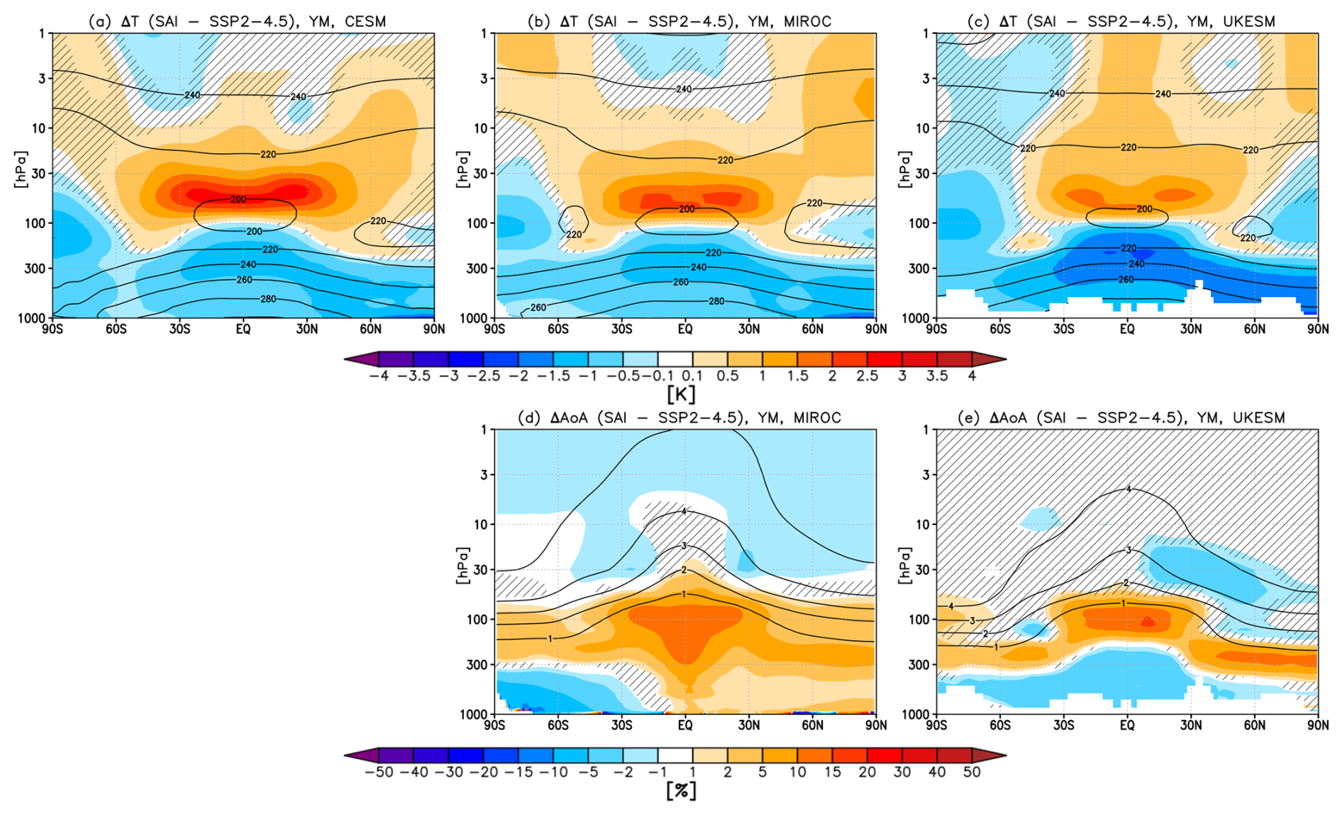
Figure 5 Shading: Annual 2045–2064 mean changes in (top, a–c) temperatures and (bottom, d–e) age-of-air between the G6-1.5K-SAI simulations and the SSP2-4.5 simulations over the same period for each model (columns). Contours show the corresponding climatological values in the SSP2-4.5 runs for reference. Hatching marks the region where the response is not statistically significant (defined as in Fig. 1). Note that an age-of-air diagnostic is not available for CESM.

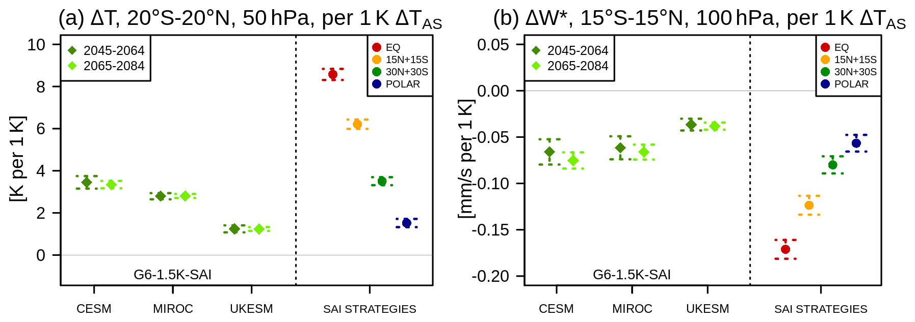
Figure 6 (a) Normalized tropical (20° S–20° N) lower stratospheric (50 hPa) temperature changes between the G6-1.5K-SAI and SSP2-4.5 simulations, averaged over either 2045–2064 or 2065–2084 periods and scaled with the corresponding global mean near-surface air temperature change. Shown also are the corresponding changes (2050–2069) in the different SAI strategies with CESM2(WACCM6-MA) (EQ, 15N + 15S, 30N + 30S, POLAR) discussed in Bednarz et al. (2023a). The error bars represent ±2 standard errors in the difference in means. (b) As in (a) but for changes in the shallow branch of the BDC, defined as in Bednarz et al. (2023a), i.e. 15° S–15° N mean of the Transformed Eulerian Mean (TEM) residual vertical velocity (w^*) changes at 100 hPa.

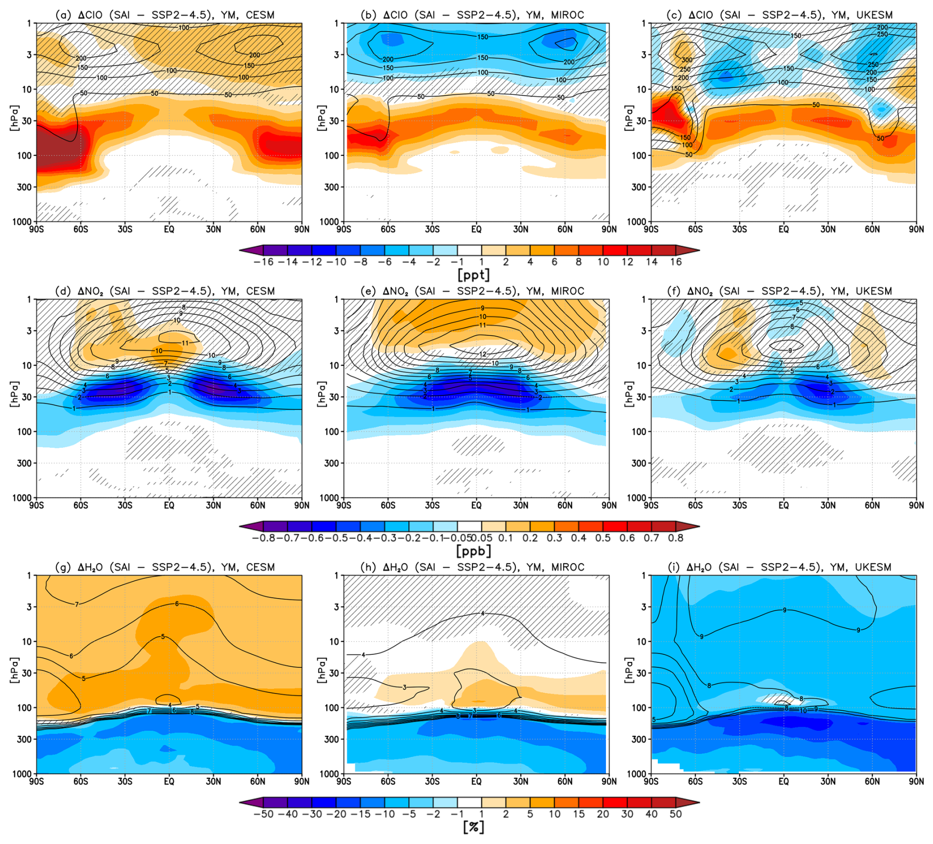
Figure 7 Shading: Annual 2045–2064 mean changes in (top, a–c) ClO, (middle, d–f) NO₂, and (bottom, g–i) water vapor, H₂O, volume mixing ratios between the G6-1.5K-SAI simulations and the SSP2-4.5 simulations over the same period for each model (columns). Contours show the corresponding climatological volume mixing ratios in the SSP2-4.5 runs for reference. Hatching marks the region where the response is not statistically significant (defined as in Fig. 1).

5 Mid-latitude ozone

As was the case with the global mean total column ozone (Sect. 3), annual mean mid-latitude total column ozone in both hemispheres increases over the 21st century under the SSP2-4.5 scenario without SAI (Fig. 8a, d). Unlike in the tropics, where the GHG-induced acceleration of tropical upwelling acts to decrease ozone, in the mid-latitudes increased transport by the BDC acts to increase ozone and thus enhances chemically-driven ozone increases due to the reduction in background halogen levels (World Meteorological Organization, 2022).

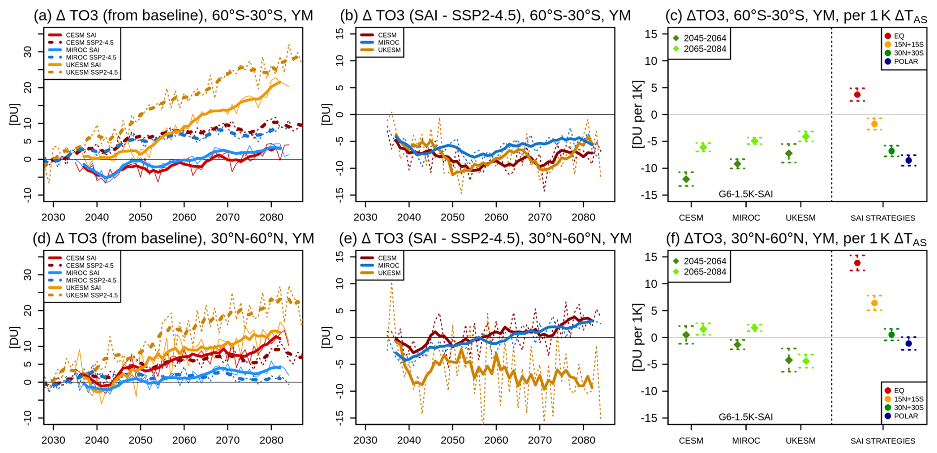
Figure 8 Annual mean (top, a–c) SH mid-latitude (60–30° S) and (bottom, d–f) NH mid-latitude (30–60° N) total column ozone changes for each of the models. (a, d) Timeseries of differences from the baseline period (2020–2039 mean of SSP2-4.5) in the control SSP2-4.5 simulations (dashed) and the corresponding G6-1.5K-SAI simulations (solid). (b, e) Timeseries of differences between the G6-1.5K-SAI and SSP2-4.5 simulations. Thin lines in (a), (b), (d), (e) denote the ensemble mean changes for each model and thick lines denote their 5-year running means. (c, f) Normalized total column ozone changes between the G6-1.5K-SAI and SSP2-4.5 simulations averaged over either 2045–2064 or 2065–2084 periods and scaled with the corresponding global mean near-surface air temperature change. Shown also are the corresponding changes (2050–2069) in the different SAI strategies discussed in Bednarz et al. (2023a; see text for more details). The error bars represent ±2 standard errors in the difference in means, calculated from the annual mean values (20 per ensemble member).

Under SAI, the impacts on mid-latitude ozone differ significantly between the hemispheres. In the SH, all three models show long-term ozone reductions of up to approx. −10 DU (with the 2045–2064 average of −7 to −9 DU SH mid-latitude ozone loss depending on the model) under SAI compared to SSP2-4.5 throughout the length of the simulation (Fig. 8b). The ozone response there is dominated by enhancement of active halogen levels in the lower stratosphere from heterogeneous reactions on sulfate (Fig. 7a–c) and the resulting acceleration of the halogen-catalyzed ozone loss. Owing to the reduction in background halogen levels with time, all models show a consistent reduction in the magnitude of the SAI-induced ozone loss per unit global temperature offset in the later period (2065–2084; −4 to −6 DU K⁻¹) compared to the earlier period (2045–2064; −7 to −12 DU K⁻¹), Fig. 8c. When comparing the SH midlatitude ozone response to different SAI strategies within CESM2(WACCM6-MA) (right side of Fig. 8c), only the equatorial injection – which shows the largest stratosphere circulation changes (Fig. 6b) and aerosol tropical confinement (not shown) – leads to an increase in the SH mid-latitude total ozone column while in the other strategies the presence of significant aerosol concentrations in the extra-tropics combined with smaller BDC changes lead to an overall reduction in the SH mid-latitude total column ozone.

A very different picture emerges for the NH mid-latitude ozone (Fig. 8d–f). Here, higher climatological lower stratospheric temperatures than in the SH (Fig. 5) slow down the rates of heterogeneous reactions on sulfate, and so any SAI-induced changes in transport can be as important in determining the overall impact on ozone. Accordingly, the three G6-1.5K-SAI models disagree more in terms of the projected effects of SAI on ozone in the NH mid-latitudes. CESM shows very little total column changes over most of the simulation, with only a small ozone increase of a few DU compared to SSP2-4.5 simulated towards the end of the experiment (Fig. 8e). MIROC shows a small ozone decrease of a few DU in the first ∼ 10–20 years followed by a similarly small ozone increase in the last ∼ 20 years. In stark contrast, UKESM shows ozone decreases of ∼ 5–10 DU throughout the simulation. These differences are likely a manifestation of large differences amongst the models in their projected chemical and dynamical responses to SAI, and their relative importance in determining the overall NH mid-latitude ozone response.

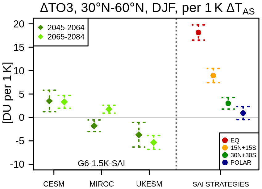
Figure 9 As in Fig. 8f but for the NH mid-latitude (30–60° N) total ozone column in boreal winter, i.e. December–January–February (DJF) mean.

These differences become even more evident when considering the analogous NH mid-latitude ozone responses in winter only (Fig. 9). Using the equatorial injection in G6sulfur simulations, Tilmes et al. (2022) and Haywood and Tilmes (2022) concluded that SAI will increase the NH mid-latitude ozone columns in winter due to the SAI-induced changes in ozone transport. However, this conclusion is not supported by the new G6-1.5K-SAI results (Fig. 9), where only CESM shows such an ozone increase (and MIROC shows a small ozone increase toward the end of the simulations only). This contrasting result is due to a number of factors. First, the 30N + 30S strategy used in G6-1.5K-SAI is associated with much smaller transport changes (Fig. 6b) and resulting dynamical impacts on ozone (Bednarz et al., 2023a), as illustrated here by the results of different strategies done with CESM2(WACCM6-MA) on the right of Figs. 9 and 8f. Second, the models appear to disagree with respect to the importance of heterogeneous chemistry versus transport for the NH mid-latitude ozone response. Only MIROC projects a significantly more negative normalized ozone response in the early (2045–2064) versus late (2065–2084) period (Figs. 8f and 9). This suggests that heterogeneous processes are not of dominant importance for determining the NH mid-latitude ozone response to SAI in CESM or UKESM, which instead likely favour more SAI-induced transport changes and dynamical impacts on ozone (which tend to scale with the amount of surface warming and stratospheric heating, Fig. 6). (It is also to be noted that the previous UKESM results in Tilmes et al., 2022; Haywood and Tilmes, 2022, had a bug in that heterogeneous processing was not occurring on SAI sulfate aerosols). Thirdly, the models appear to show important differences in their projected SAI-induced changes in transport (both BDC and mixing) and the resulting impacts on ozone, with CESM showing transport changes that act to increase the NH mid-latitude ozone and UKESM simulating transport changes that acts to decrease the NH mid-latitude ozone. Further evidence of different transport changes and the net effects of varying BDC and mixing changes between models can also be seen when comparing the model age-of-air changes (Fig. 5d–e), with MIROC showing increases in age-of-air (i.e. older air) extending throughout the lower stratosphere and UKESM showing such increases limited to the tropics and the UTLS region while the extra-tropical lower stratosphere shows younger age-of-air instead (especially in the NH). See Sect. 7 for more analysis of the relative importance of dynamical versus chemical process for the ozone response to SAI in UKESM. Importantly, the differences amongst the models here with respect to the projected NH mid-latitude ozone impacts, as well as contrasting conclusions to those made previously based on G6sulfur results in Tilmes et al. (2022), highlight the still very large model uncertainties in the projected SAI impacts, including at the process level, and underscores the need to further assess such impacts in the wider strategy and scenario dimension as well as in a multi-model framework.

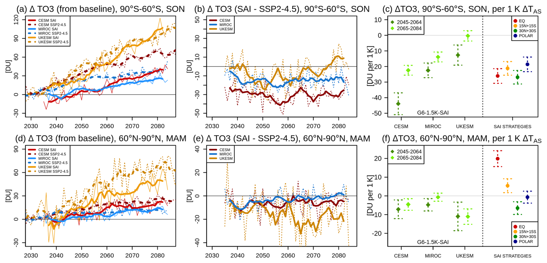
Figure 10 Springtime (top, a–c) SH high-latitude (90–60° S, September-October-November, SON) and (bottom, d–f) NH high-latitude (60–90° N, March–April–May, MAM) total column ozone changes for each of the models. (a, d) Timeseries of differences from the baseline period (2020–2039 mean of SSP2-4.5) in the control SSP2-4.5 simulations (dashed) and the corresponding G6-1.5K-SAI simulations (solid). (b, e) Timeseries of differences between the G6-1.5K-SAI and SSP2-4.5 simulations. Thin lines in (a), (b), (d), (e) denote the ensemble mean changes for each model and thick lines denote their 5-year running means. (c, f) Normalized total column ozone changes between the G6-1.5K-SAI and SSP2-4.5 simulations averaged over either 2045–2064 or 2065–2084 periods and scaled with the corresponding global mean near-surface air temperature change. Shown also are the corresponding changes (2050–2069) in the different SAI strategies discussed in Bednarz et al. (2023a; see text for more details). The error bars represent ±2 standard errors in the difference in means, calculated from the annual mean values (20 per ensemble member).

6 Springtime polar ozone

The following section discusses changes in springtime polar ozone in both hemispheres. Given the interplay of chemical and dynamical processes, the springtime Antarctic saw the largest historical ozone losses due to anthropogenic emissions of long-lived ODSs (World Meteorological Organization, 2022). Consequently, it is projected to see the largest increases in total column ozone over the 21st century as background halogen concentrations decline (Fig. 10d; see also e.g. Dhomse et al., 2018; Keeble et al., 2021).

Under SAI (Fig. 10b), all three models show relative decreases of Antarctic total column ozone compared to SSP2-4.5 (though UKESM starts to show a small increase relative to SSP2-4.5 around 2070s). The ozone losses are about twice as large in CESM (−33 DU on average between 2045–2064) compared to MIROC (−16 DU) and UKESM (−15 DU). The differences in magnitude become even larger when the magnitude of ozone loss is normalized with the associated SAI-induced global mean surface cooling, with −44 DU K⁻¹ loss in CESM, followed by −22 DU K⁻¹ in MIROC and −13 DU K⁻¹ in UKESM (Fig. 10c), highlighting substantial structural uncertainty in the magnitude of this SAI “side-effect” on Antarctic ozone. When normalized with the associated annual mean SO₂ injection rate, these Antarctic ozone losses range between −4.7 DU per Tg-SO₂ yr⁻¹ to −1.4 DU per Tg-SO₂ yr⁻¹. Importantly, all three models project that the normalized ozone loss in the later part of the century (2065–2084) becomes a factor of ∼ 2 smaller than earlier in the century (Fig. 10c; ranging from −22 to 0 DU K⁻¹ and −2.4 to 0 DU per Tg-SO₂ yr⁻¹), in line with lower background halogen concentrations available for activation on sulfate. Unlike changes in global mean and mid-latitude ozone (Sects. 3 and 5), where the choice of SAI strategy was found to play a much larger role in determining both the sign and magnitude of ozone response than inter-model uncertainty, the inter-model spread of Antarctic springtime total column ozone responses by far outweighs the uncertainty stemming from the choice of SAI strategy alone (Fig. 10c).

Nonetheless, we find a very strong correlation ($R=-\mathrm{0.949}$) between the magnitude of the SAI-induced springtime Antarctic ozone loss and the strengthening of the austral polar vortex across the three different models and two time periods (Fig. 11a, c). This correlation is even stronger ($R=-\mathrm{0.974}$) if annual mean stratospheric wind changes are considered instead (Fig. S4). The inter-model spread of magnitudes of the Antarctic polar vortex strengthening (Fig. 11a) is closely related to the inter-model spread of the magnitudes of the associated tropical lower stratospheric heating (Fig. 6a) as aerosols absorb infra-red radiation, with models with a larger tropical heating also showing a stronger Antarctic polar vortex strengthening. A similar relationship has also been found for the different SAI strategies in Bednarz et al. (2023a), as shown here in the right-hand-side parts of Figs. 11a and 6a. However, unlike the normalized magnitude of the tropical lower stratospheric heating – which, as expected, does not change between the early and late periods (Fig. 6a) – the normalized magnitude of the Antarctic vortex strengthening is consistently larger in early period (2045–2064) than late period (2065–2084) in all three models, thus following the behaviour of stratospheric ozone response (Fig. 10c). Such a close relationship between springtime Antarctic ozone and polar vortex arises because changes in Antarctic ozone drive changes in polar stratospheric temperatures that modulate the strength of the polar vortex, and conversely, changes in polar vortex strength are associated with both changes in polar stratospheric temperatures that control chemical ozone loss as well as with changes in ozone transport and mixing. A similar relationship between changes in polar ozone and vortex strength has been also previously found in the context of impacts of ODSs and GHG (e.g., McLandress et al., 2010; Zhang et al., 2017; Butler and Domeisen, 2021). Our study thus constitutes the first demonstration that such a relationship would also exist in the context of SAI impacts, thus providing a potential constraint to narrow the uncertainty in SAI impacts in the Antarctic across different models.

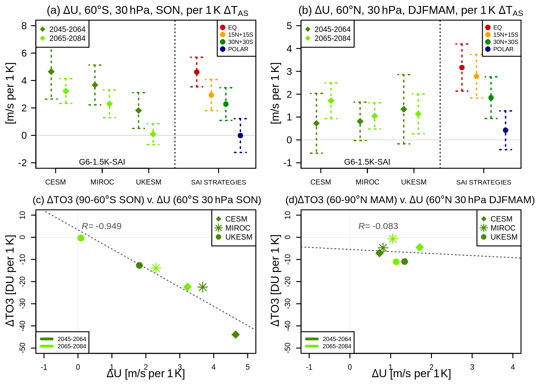
Figure 11 Top (a–b): As in Fig. 6 but for the normalized changes in the stratospheric polar vortex strength during dynamically active seasons, calculated as changes in zonal mean zonal wind at 30 hPa and either 60° S in SON (a, for the Antarctic polar vortex) or 60° N in DJFMAM (b, for the Arctic vortex). Bottom (c–d): Correlation between the normalized changes in the springtime high latitude total column ozone (as in Fig. 10c, f) and polar vortex strength during dynamically active season (as in panels a–b here) in the G6-1.5K-SAI simulations for Antarctic (c) and Arctic (d).

A different picture emerges for Arctic ozone (Fig. 10d–f). CESM and MIROC both show moderate springtime Arctic ozone decreases of up to approx. −10 DU compared to SSP2-4.5 that are largest earlier in the century and then decrease with time (Fig. 10e). On the other hand, UKESM shows much larger ozone decreases of approx. −10–30 DU that persist with time, similar to what was seen for the NH mid-latitude ozone (Fig. 8e). Regarding the relationship with the concurrent winter-to-springtime (December-to-May, DJFMAM) polar vortex changes, while all three models show overall strengthening of the Arctic vortex under SAI (Fig. 11b), no obvious relationship is found with the springtime Arctic ozone loss across the three models and two time periods (Fig. 11d). In general, while changes in Arctic ozone have been found to be connected to changes in Arctic polar vortex strength under different contexts (Bednarz et al., 2016; Friedel, 2022a, b; Chiodo et al., 2023; Kult-Herdin et al., 2023), such correlations tend to be more difficult to detect, and this could be partly because of much larger variability of the NH polar vortex, both in time and space, thus making such a relationship more difficult to diagnose using monthly and zonal mean data.

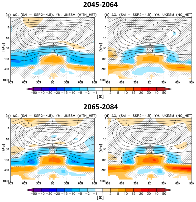
Figure 12 Shading: Annual (top, a–b) 2045–2064 mean and (bottom, c–d) 2065–2084 mean changes in ozone volume mixing ratios between the UKESM G6-1.5K-SAI simulations and the SSP2-4.5 simulations over the same period. Left (a, c) is for the fully coupled simulation discussed in the paper (as in Fig. 4), and right (b, d) is for the analogous simulation without heterogeneous chemistry on SAI sulfate aerosols. Contours and shading as in Fig. 4.

7 Diagnosing the role of heterogeneous chemistry versus transport in UKESM

Attributing stratospheric ozone changes under SAI to specific dynamical and chemical processes, in particular disentangling the relative importance of accelerated heterogeneous chemical processing on sulfate versus dynamically induced ozone changes, in fully coupled simulations remains inherently difficult. For that reason, in this final section we compare the results of the fully-coupled UKESM simulations discussed in the previous sections with the results of the analogous simulations that do not include heterogeneous chemistry on SAI sulfate aerosols (which are the original UKESM G6-1.5K-SAI simulations discussed in Lee et al., 2026). As discussed in Sect. 2, while the two sets of simulations have slightly different injection rates (10.7 vs. 10.3 Tg-SO₂ yr⁻¹ for 2045–2064 and 15.7 vs. 14.5 Tg-SO₂ yr⁻¹ for 2065-2084 using the simulations in Lee et al. (2026) vs here, respectively) and surface cooling values (−1.1 vs. −1.2 K for 2045–2064 and −1.8 vs. −1.9 K for 2065–2084 using the simulations in Lee et al. (2026) vs. here, respectively), those effects are not expected to lead to first-order differences in the simulated ozone responses and so the dominant differences will be driven by the presence or absence of heterogeneous chemistry on sulfate from SAI.

Figure 12 shows annual mean ozone changes in UKESM for 2045–2064 (top) and 2065–2084 (bottom) between G6-1.5K-SAI and SSP2-4.5 over the same period, with panels (a, c) being for the fully coupled experiment discussed throughout the manuscript (here denoted “WITH_HET”) and panels (b, d) for the corresponding simulations without heterogeneous chemistry on SAI sulfate (denoted “NO_HET”). As expected, both sets of simulations show tropical ozone increases in the lower stratosphere due to the SAI-induced deceleration of upwelling in the UTLS and shallow BDC branch. In addition, while the fully coupled simulations show decreases in polar ozone in both hemispheres driven by the halogen-catalyzed chemical ozone loss and its coupling with circulation (Sect. 6), the simulations without heterogeneous chemistry on SAI sulfate do not show such polar ozone reductions. However, in the off-equatorial tropical and mid-latitudes, the NO_HET simulations also show ozone decreases in the lower stratosphere resembling those in the fully coupled simulations but of lower magnitude. These lower stratospheric ozone losses contribute to the corresponding changes in total ozone columns (Figs. 13a, S5), especially if only stratospheric ozone columns are considered (Fig. 13b; here approximated as altitudes of 150 hPa and above to remove the offsetting positive ozone changes in the extra-tropical UTLS under SAI-induced lowered tropopause).

This shows that while heterogeneous chemical processing on SAI sulfate is partially responsible for the ozone losses in the subtropical and mid-latitudes in the fully coupled run, a second important contribution comes from the SAI-induced changes in transport, at least in UKESM. Such ozone decreases likely arise here due to enhanced transport of ozone poor-air from the tropical lower stratosphere (as also suggested by the corresponding changes in model age-of-air pointing towards younger air in the regions with lower ozone, Fig. S6), either as the result of acceleration of the BDC above the aerosol layer (likely responsible for the ozone losses in the subtropics at ∼ 50–30 hPa) and/or enhanced isentropic mixing (likely responsible to the ozone losses in the mid-latitudes ∼ 100–50 hPa). Given the disagreements between the three G6-1.5K-SAI models regarding their projected SAI impacts on ozone in the NH mid-latitudes (Sect. 5), thereby pointing to model differences in the representation of transport processes and their response to SAI, the results highlight some prevailing process level uncertainties – in this case relating to the details of SAI-induced modulation of transport – that needs to be addressed and narrowed.

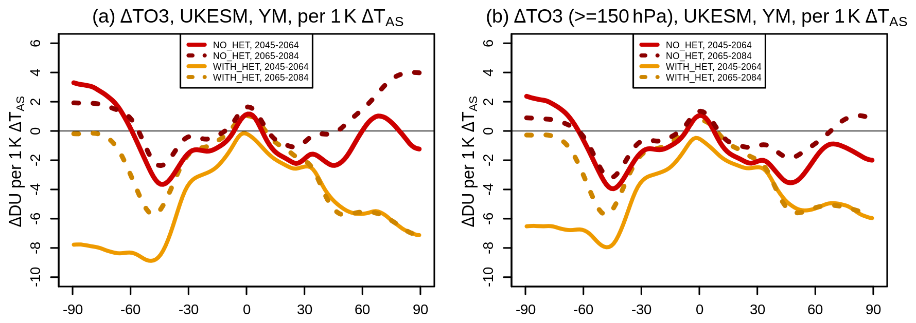
Figure 13 Normalized annual mean total (a) and stratospheric (b, here taken as altitudes of 150 hPa and above) column ozone changes per 1 K global mean near-surface air cooling in the UKESM simulations with heterogeneous chemistry on SAI sulfate aerosols included (yellow, WITH_HET) and the analogous simulations without it (red, NO_HET) for 2045–2064 (solid) and 2065–2084 (dashed) as a function of latitude.

8 Summary and conclusions

Stratospheric Aerosol Injection (SAI) using sulfate aerosols, a proposed method of temporarily offsetting a portion of anthropogenic climate change, is recognized to affect the ozone layer (e.g. Haywood and Tilmes, 2022). In this paper we provide an assessment of SAI impacts on the ozone layer and stratospheric ozone projections over the 21st century using the new GeoMIP G6-1.5K-SAI multi-model experiment. The experiment constitutes an advance on the older GeoMIP G6sulfur experiment by utilizing a symmetric injection of SO₂ at a pair of subtropical latitudes (30 and 30° N), as opposed to the equator, as well as a more plausible middle-of-the-road GHG scenario and SAI start date.

All three comprehensive Earth system models with fully coupled aerosols and chemistry that performed this experiment – CESM2(WACCM6), MIROC-ES2H and UKESM1.1 – project a decrease in global mean total column ozone in G6-1.5K-SAI relative to SSP2-4.5 of a few DU. This is in contrast to previous simulations that utilized SAI strategies injecting in the equatorial region, which tend to induce an increase in global mean ozone, largely due to a larger SAI impact on stratospheric circulation (especially BDC) and ozone transport. In the case of subtropical injections (30° N and 30° S, as examined here), SAI impacts on circulation are much smaller, and so the global mean column ozone response is dominated by – now larger – lower stratospheric ozone decreases from increased active halogen levels driven by heterogeneous chemistry (both halogen and nitrogen processing) on sulfate and the resulting enhancement of the halogen catalyzed ozone loss in the lower stratosphere. Owing to the continued reduction in background stratospheric halogen levels over the 21st century available for activation, all three models consistently simulate much larger (factor of ∼ 2) potential of SAI to deplete ozone (taken as global mean ozone loss normalized per degree of the associated global mean surface cooling) in the earlier part of the 21st century than later (∼ −4 DU K⁻¹ in 2045–2064 compared to ∼ −1–2 DU K⁻¹ in 2065–2084). The results illustrate that whilst the sub-tropical injection strategy employed in G6-1.5K-SAI might have fewer adverse effects on aspects of regional surface climate compared to earlier strategies, e.g. in G6sulfur, injecting at the equator (e.g. Lee et al., 2026; Zhang et al., 2024), for stratospheric ozone it is projected to lead to an overall global mean ozone reduction and thus potentially a less favourable outcome (Fig. S7; see also discussion below), highlighting potential trade-offs of different SAI choices. Furthermore, by comparing the multi-model G6-1.5K-SAI experiment with a multi-SAI strategy ensemble from one model, we have shown how the choice of SAI strategy can have a much larger role in determining the global mean total column ozone response to SAI than the inter-model uncertainty.

At regional scale, the models agree that SAI will lead to a reduction in annual mean total column ozone in the SH mid-latitudes compared to SSP2-4.5 (at larger magnitude than for global mean ozone), likely dominated by the halogen activation from heterogenous processing on sulfate. In contrast, although SAI-induced total column ozone changes in the tropics and the NH mid-latitudes are modest in absolute terms, models disagree on their sign and magnitude. This arises because SAI induced ozone changes in these regions are caused by the interplay of a number of chemical and dynamical processes, and the models disagree in terms of their relative importance under SAI. We further find that the conclusion of Tilmes et al. (2022) based on the G6sulfur simulations in that the NH mid-latitude ozone columns will increase under SAI, especially in winter, no longer holds in G6-1.5K-SAI. This is likely due to the combination of different SAI strategy used and inter-model differences in the simulated transport changes under SAI, although differences in GHG and SAI scenarios could be a further potential contributing factor.

Regarding changes in springtime polar ozone, all three models show a relative decrease of Antarctic springtime total column ozone compared to SSP2-4.5 throughout the length of the simulation, but with substantial differences in the magnitude of this decrease across the models. For the 2045–2064 mean, the magnitudes of the springtime Antarctic total column ozone loss per degree of global mean surface cooling range between −44 DU K⁻¹ in CESM to −13 DU K⁻¹ in UKESM. Nonethless, all models agree that the normalized ozone loss in the later part of the century (2065–2084) becomes a factor of ∼ 2 smaller than earlier in the century, in line with lower background halogen concentrations available for activation on sulfate. Importantly, we find a very strong correlation ($R=-\mathrm{0.95}$) between the simulated Antarctic springtime total ozone column loss and the associated strengthening of the SH stratospheric polar vortex across the three models and two time periods (hence background halogen levels). Similar relationships between changes in Antarctic ozone and the polar vortex strength have been found in other contexts, and our study thus provides the first demonstration that such a relationship would also exist in the context of SAI impacts, thus providing a potential constraint to narrow the uncertainty in SAI impacts in the Antarctic across the models. For the Arctic, models simulate decreased springtime Arctic ozone under SAI compared to SSP2-4.5, but with no clear correlation to either the strength of the Arctic winter-to-spring polar vortex or time period. This behaviour could be due to much larger variability characterizing the Arctic stratosphere and hence difficulty in detecting any such relationship in general, especially using monthly and zonal mean data.

By analyzing the roles of atmospheric transport versus chemistry for the SAI ozone response in UKESM, we demonstrate how altered circulation and ozone transport under SAI make an important contribution to the subtropical and mid-latitude ozone losses in the model. In conjunction with the disagreement amongst the different models in terms of the sign of the projected NH mid-latitude ozone responses to SAI, the results highlight some of the still prevalent process level uncertainties regarding SAI impacts on atmospheric circulation, including the relative interplay and importance of altered residual circulation and mixing. Inconsistencies between climate model simulations and observations regarding changes in mid-latitude lower stratospheric ozone, including even their sign, has also been found in the context of recent ozone trends (e.g. Dietmüller et al., 2021; Ball et al., 2020); while the reasons behind those differences are still not fully understood, some evidence points to the models' deficiencies in simulating the details of recent stratospheric transport changes (BDC and mixing) under changing climate. All of these thus underscore the need to improve and constrain climate model representation of stratospheric transport, which will also have broader implications for wider range of contexts, including impacts of explosive volcanic eruptions (e.g. Bednarz et al., 2026) or space industry (e.g. Maloney et al., 2025).

Importantly, the SAI impacts discussed in this paper are largely shown as changes relative to the SSP2-4.5 simulation over the same time period. The ozone decreases due to SAI emerge within a few years from the onset of SAI, and thereafter stratospheric ozone continues to recover (i.e. increase) over the course of the 21st century, just lagging the ozone evolution projected under the no-SAI scenario, at least until near the end of the 21st century. In addition, any SAI-induced ozone losses are likely to be smaller than any losses from peak ODS-induced depletion (e.g. Dhomse et al., 2018). Furthermore, SAI discussions often assume that impacts of any future SAI-induced ozone reduction on human and ecosystem health will be strictly negative, and impacts of any SAI-induced ozone increase will be strictly positive. However, decreasing ODSs and increasing GHGs under SSP2-4.5 are projected to lead to ozone “super-recovery” compared to historical levels (and even more under higher GHG emission scenarios, World Meteorological Organization, 2022). Yet, human impacts of the projected ozone super-recovery are still not well understood, including the interplay of both negative and positive impacts from UV exposure, e.g. on skin cancer and vitamin D production, as well as health implications from changes in surface ozone exposure (see e.g. United Nations Environment Programme, 2023, 2024). Hence, implications of any SAI-induced ozone changes need to be studied properly and carefully weighed against the uncertainties in full health and ecosystem implications of such baseline ozone super-recovery.

All in all, our results highlight the need to assess SAI impacts on atmospheric composition and circulation in the wider strategy and scenario dimension using a multi-model framework.