A cellular automaton model of tropical oceanic rain clusters with criticality

The distributions of the cluster area, A, and total rain rate, R, for tropical oceanic rain clusters from a cellular automaton (CA) are analysed for their scaling exponent ζ_A, ζ_R, and β where f(s) ∼ $s^{-{\mathit{\zeta }}_{\mathrm{S}}}$; $S\in \mathit{\{}A,R\mathit{\}}$; f(s) the probability distribution of S; β is that for rain rate conditioned by rain area. The CA only includes a few simple rules representing a small set of dynamics thought to be important for convective organization. These rules represent large-scale destabilization of the atmosphere under the moisture static energy framework with a slow driving timescale, as well as convective cells interaction through propagating gravity waves with a fast relaxation timescale. The CA exhibits percolation-like criticality, and the ζ_A is estimated to be near the theoretical 2-dimensional percolation value of 187/91. This agrees well with the ζ_A estimates over the Indian Ocean warm pool and the tropical Atlantic reported in previous modelling study, implying numerical models behave like percolation. Although other critical exponents of the rain cluster distributions from the CA, namely the η_S (scaling exponent of the characteristic scale) and D_S (cluster fractal dimension), $S\in \left(\left.A,R\right\}\right.$, depend on the adjustable parameter of the CA, the ζ_A is robust to the adjustable parameter. Although the CA cannot account for the observation-based ζ_A ∼ 5/3 reported elsewhere that is quite universal over all oceans, further tuning of it such as through the convective cells interaction strength or how they interact may allow the CA to produce the observed exponent. Whether such behaviour can arise from a genuinely self-organized mechanism, rather than through parameter tuning, remains a question for future investigation.

1 Introduction

It has long been recognized that clouds and rain possess the phenomenon of “clumping” (Randall and Huffman, 1980). In other words, clouds and rain seem able to self-organize or self-aggregate into clumps, more often referred to as clusters, from small convective cells, although such organization not necessarily implies reduction in complexity from the perspective of information entropy (see Li et al., 2019). With clumping, cloud cluster sizes follow power laws in form, f(s) ∼ $s^{-{\mathit{\zeta }}_{\mathrm{S}}}$, f(s) being the distribution of some observables of the clouds or rain, and ζ_S a positive scaling exponent (López, 1977, 1978; Lovejoy, 1982; Cahalan and Joseph, 1989; Peters et al., 2009, 2010; Wood and Fields, 2011; O'Brien et al., 2013; Devineni et al., 2015; Traxl et al., 2016; Teo et al., 2017; Otsuka et al., 2017; Neggers et al., 2019; Li et al., 2022; Savre and Craig, 2023). Besides theoretical interests, recent studies also demonstrated that convection organization is a critical factor determining the characteristics of extreme precipitation (Bao et al., 2017; Pendergrass, 2020; Semie and Bony, 2020; Roca and Fiolleau, 2020; Zhang and Wang, 2021) and tropical cyclogenesis (Muller and Romps, 2018).

It has been further suggested that tropical convective rain could be a critical phenomenon (Peters and Neelin, 2006; Peters et al., 2009; but cf. Muller et al., 2009), which provides a basis to understand what controls the power-law distributions seen in observations and models. In the specific framework of self-organized criticality (SOC) (Bak et al., 1987), such behaviour arises spontaneously without external parameter tuning, and the critical exponents such as ζ_S for a certain observable would be universal, should be seen in the distributions across observations and numerical models, and depending only on a few fundamental physical constraints rather than on the detailed interactions and microphysical processes. However, it is important to note that power-law statistics alone do not uniquely imply SOC; similar scale-invariant behaviour can emerge from a variety of multiscale dynamical processes, including tuned critical phenomena (where a control parameter must be finely adjusted) or absorbing-state phase transitions (Dickman et al., 1998; Vespignani and Zapperi, 1998). In the present study, we do not claim that the CA exhibits SOC in the strict sense; rather, we use it as a controlled testbed to investigate which physical mechanisms may drive the system toward criticality and to examine the resulting scaling exponents.

Peters et al. (2009) suggests that tropical oceanic rain clusters behave geometrically like 2-dimensional percolation clusters (Broadbent and Hammersley, 1957), and consequently for the rain cluster area, S = A, ζ_A = 187/91, in principle (Stauffer and Aharony, 1994). Estimated value in Peters et al. (2009) from observations is about 2 appears to agree with percolation theory. Universality of observed rain clusters has been reported by Teo et al., 2017 (abbreviated as T17 hereafter) where the estimated ζ_A across the tropical basins are the same, but they reported a lower estimated value of ζ_A ∼ 5/3. Otsuka et al. (2017) through analysis of model rain clusters reported a power-law scaling for the rain cluster area when light rain is included and an exponent of 5/3 for the distribution of cloud shield area. Analysis of multi-year model rain clusters over the various different oceanic basins is needed for a more informed comparison with existing results in the literature.

In general, there are two approaches to investigate the self-aggregation processes and associated statistics of cloud/rain clusters. First is through dynamical modelling, often with Radiative Convective Equilibrium (RCE) and cloud-resolving resolution (Wing and Emanuel, 2014; Wing et al., 2017; Savre and Craig, 2023; Cerlini et al., 2023; Stephan and Stevens, 2025). The second is a “reductionist” approach that applies cellular automata (CA), which simplifies the physical and dynamical processes as deterministic or stochastic transition “rules” of lattice cell states in the model. With less computational resources necessary than in dynamical models, CA are able to study the critical behaviour of the observables represented in the models and facilitate comparison across a wide range of natural phenomena (Malamud and Turcotte, 2000). Previous applications of CA to study cloud clusters varied substantially in terms of how cloud processes are represented, although they are all fluid dynamics based. The early model of Nagel and Raschke (1992) focused on the interaction between cloud water vapor, humidity and vertical velocity represented in the model cells. Comparatively, the Silva et al. (2019) model is quite “realistic” in that it replicated condensation processes as well as advection by winds across the cells. Recently, the model in Najafi et al. (2021) and Cheraghalizadeh et al. (2024) also emulated microphysical processes in clouds and at the same time considered the cohesive energy of clouds resembling cell interaction in the Ising model.

In addition to these physically motivated CA models, a parallel line of research has focused on using CA as a stochastic parameterization tool within numerical weather prediction (NWP) models to represent subgrid convective organization and its uncertainty (Palmer, 1997, 2001; Bengtsson et al., 2011, 2013, 2019, 2021, 2022; Bengtsson and Han, 2024; see also Nober and Graf, 2005; Graf and Yang, 2007). These studies have demonstrated that CA-based stochastic schemes can improve the representation of convectively coupled equatorial waves, Madden–Julian oscillation propagation, and ensemble spread in operational forecast systems. However, their emphasis is on forecast skill rather than on understanding the fundamental scaling properties of rain clusters.

Other reduced-complexity models have approached convective organization from different physical perspectives. Craig and Mack (2013) developed a coarsening model based on free-tropospheric moisture budget, drawing analogy with phase separation in materials science. Ahmed and Neelin (2019) adopted a stochastic modelling approach that was based on the noise-driven moisture–weak temperature gradient (WTG) equation. Their model was on a 2-dimensional plane and represented processes from large-scale circulation to storm internal dynamics as well as precipitation parameterization. Thus, their approach was more like a NWP model, with the benefits of a large variety of sensitivity tests. Indeed, cluster area and rain scaling exponents very close to those found in T17 were reproduced. Ahmed and Neelin (2019) also discussed that why they intended to exclude site percolation as a framework for precipitation clustering, mainly based on the fact that the cluster scaling exponents are sensitive to grid size and that there was no clear physical scale corresponding to the cutoff (deviation from power law) in percolation model. Nevertheless, as will be seen in the following, our approach is to develop a convective physics-based SOC model with near-field dynamics and relationships to the cluster scaling exponents, rather than from a pure percolation approach. Biagioli and Tompkins (2023) proposed a stochastic reaction–diffusion lattice model that predicts the onset of self-aggregation through a dimensionless “aggregation number”. More recently, Neggers and Griewank (2021, 2022) formulated the BiOMi (Binomial Objects on Microgrids) framework, which models populations of interacting convective thermals on a two-dimensional grid and couples them to a spectral convection scheme to capture spatial organization and its impact on vertical transport. While these models offer valuable insights into different aspects of convective organization, from onset prediction to population dynamics, they have not systematically examined the critical scaling exponents of rain cluster size and rain rate distributions, which are the focus of the present study.

Here we develop a CA based on atmospheric stability measured by the moist static energy (MSE; Yao et al., 2022). Our study is a step forward from previous observational analysis (T17) and model simulations (Teo et al., 2021, hereafter T21), which postulated rain clusters as avalanching sand-piles as in the self-organized criticality (SOC; Bak et al., 1987) theory. T17 and T21 analysed rain cluster distribution for its scaling exponents ζ_A, ζ_R and β (for rain area, rain rate and area-conditioned rain respectively; See Appendix A for details). Our model exhibits critical behaviour when the large-scale drive is tuned to a specific value, and its cluster statistics resemble those of systems near a critical point, reminiscent of the behaviour hypothesized for tropical rainfall (Peters and Neelin, 2006; Peters et al., 2009; Stechmann and Neelin, 2014; T17). However, as we will discuss in Sects. 2–4, the CA requires fine-tuning of the external drive to reach criticality, placing it in the category of tuned critical phenomena rather than SOC in the strict sense. This distinction is important: the value of the CA lies not in demonstrating SOC per se, but in enabling a controlled investigation of how specific physical processes (e.g., gravity wave interactions in our model) influence the emergent scaling exponents of rain clusters. Through such a CA model, we hope to elucidate the important factors that may cause the rain clusters to be critical, and its result would be useful in interpreting the distributions of the rain clusters seen in observations and numerical weather models.

The remaining of the paper is as follows. Section 2 introduces the CA for tropical oceanic rain cluster. Analysis of the model's cluster distributions is presented in Sect. 3. Further discussions on the implications of our findings are in Sect. 4 before summarizing our work in Sect. 5.

2 CA for tropical rain clusters

2.1 Large-scale destabilization and convective toppling (relaxation)

In this section, we give an overview of the CA for the tropical rain clusters use in this study. In the interest of clarity, the bulk of the mathematical details is presented in Appendix B. The rules of the CA are summarized in Table 1. The CA is defined on a square lattice with open boundaries. For lattice size Z, we consider the data resolution that was analysed in T17 (25 km satellite-estimated rain) and T21 (36 km numerical model simulation). While Z = 120 and Z = 96 was applied in T17 and T21 respectively, which were large enough to cover each of the tropical oceanic regions with deep convection, we extend the lattice size to Z = 512 for the CA here such that scaling up to very large rain clusters can be realized. The main prognostic non-dimensional variable at each lattice site, X, represents the stability of the column of atmosphere against moist convection over a homogeneous ocean surface. In this simple model, X is taken to be the difference between the boundary-layer (below ∼ 850 Pa) averaged specific moist static energy, h₁, and the layer-averaged specific saturated moist static energy at the top of the troposphere (above ∼ 450 hPa), $h_{\mathrm{3}}^{*}$ (Fig. 1). By assuming that h₁ and $h_{\mathrm{3}}^{*}$ are larger than the layer-averaged saturated specific moist static energy of the middle troposphere (denoted as h₂; Eq. B1) at all times, deep convection (and consequently precipitation) only occurs at a lattice site j if X_j is positive (Eq. B2); no deep convection is triggered otherwise. In this model, X is bounded below at a value arbitrarily set to −1, after normalized by a maximum stability, X_o, that the atmosphere can attain. Large-scale forcing gradually destabilizes the atmosphere through surface fluxes and radiative cooling, represented by adding a predefined increment, d, to X at each driving cycle (Eq. 1). The driving timescale, t_LS, is much longer than the convective relaxation timescale, ensuring separation of scales.

Table 1 The rules for the CA on a square lattice with N grid points. The dynamic variables of the model, X, ΔX are functions of two time coordinates. t denotes the outer time (radiative timescale) while τ denotes the microscopic time (convective timescale). τ_F(t) is the final microscopic time at quiescence after the tth avalanche, where τ_F(0) = 0 by definition. g is a predefined random variable defined on $[-\mathrm{1},\mathrm{0}]$ as the X attained after toppling whose distribution is shown in Fig. B2. Equations (3) and (4) represent the relaxation process to stable condition after toppling. Refer to Appendix B for the physical basis for the equations.

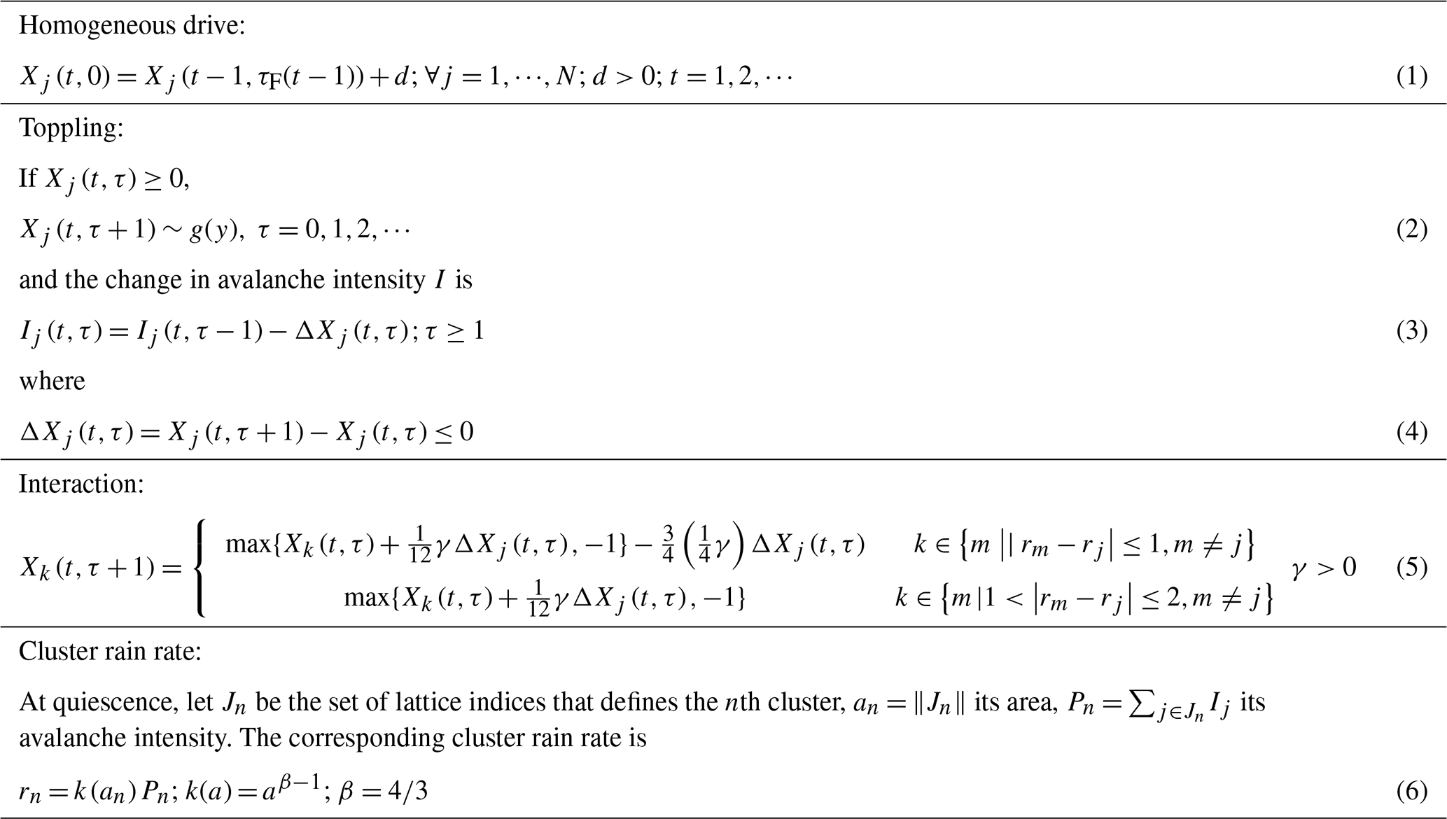
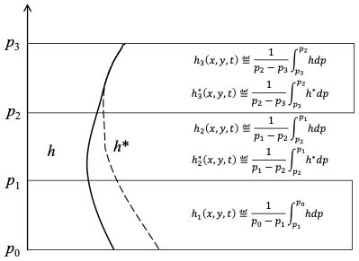
Figure 1 Illustration of the moist static energy profiles in the CA. Vertical axis is the atmospheric pressure. P₀, P₁, P₂ and P₃ are 1000, 850, 450, and 100 hPa, respectively. See Appendix B for more details on how the CA variable X is defined from these unsaturated and saturated profiles.

The CA operates in the following manner: at each outer or radiative time step t, X is increased by a value d at all lattice sites, representing the large-scale destabilization of the atmosphere due to the combined effects of latent heat fluxes in the boundary layer and net radiative cooling of the atmosphere (Eq. B3). The rate of change is 5.768 kJ kg⁻¹ d⁻¹ based on estimates from the literature (Appendix B1). For the unstable (toppling) sites with X > 0, deep convection is assumed to restore the local stability, represented in the model by relaxing their X immediately (after a microscopic or convective time step τ) back to some negative values. This relaxation represents the combined effects of convective transport and compensating downdrafts (Eqs. 2–4). These relaxed X values are drawn stochastically from a distribution g(x) estimated from published literature (see Appendix B2 for the estimation of g) to reflect the uncertainties introduce by various cloud processes during deep convection. Driving of all the model sites is only resumed after all toppling activities complete, after which all sites become stable again and the system as a whole is in equilibrium. Then the cluster statistics are analysed. As will be seen in the following, such separation of time scales (t and τ) is critical to the rain cluster size distributions simulated in the CA.

2.2 Gravity wave interactions

A raining (toppling) site in the model is assumed to interact with its neighbouring sites through two modes of horizontally propagating gravity waves excited by the latent heating profile at the site where the deep convection occurs. The first set of gravity wave, GW1, is excited at the mature stages of the deep convection when the maxima latent heating is at the mid-troposphere, while the second set of gravity wave, GW2, is excited at the later stage of the storm development when the heating maxima is higher up and presumably accompanied by evaporative cooling at the lower troposphere. These gravity waves are assumed to radiate horizontally away from the convective site with circular wavefront, with the phase speed of GW2 half of that of GW1 since the vertical wavelength of the earlier is taken to be about half of the latter (Fig. 2). GW1 acts to stabilize the atmosphere while the presence of GW2 acts to destabilize the atmosphere behind its wavefront. The effects of these gravity waves are represented in the CA by increasing X (destabilize) for the nearest-neighbours and decrease X (stabilize) for the next-nearest-neighbours of a toppling site (Eq. 5). The magnitude of the (de)stabilization of the (nearest-neighbour) next-nearest-neighbour is proportional to $\left|\mathrm{\Delta }X\right|$ at the precipitating site with a tunable positive constant γ, which represents the degree of coupling between different locations by gravity wave dynamics (Appendix B3). Note that in this scheme of gravity wave effect, treatment is site-by-site and thus only near-field effect has been simulated, considering that the grid size in the lattice is around 30 km (as mentioned in Sect. 2.1). As such, the propagation speed of gravity waves has been considered in our model to a certain extent. In reality, convective cells form a cluster and collectively a strong gravity wave may propagate from the convective tower as a whole and influence the far field (i.e., longer range than the next nearest neighbour). We only simulate the near-field effect because that is more in accord SOC models, which generates long-range spatial correlation from short-range interaction. From another perspective, full-physics simulations in T21 using WRF still generated scaling exponents of cluster area and rain rate with deviations from those observed. Thus, we experiment with idealized, near-field interactions in the CA here.

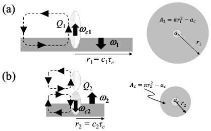
Figure 2 Schematic showing the effects on the atmosphere due to the (a) GW1 (ℓ = 1) and (b) GW2 (ℓ = 2) gravity bores. The diagrams on the left represent a vertical cross-section of the troposphere that includes the convective site. The vertical (horizontal) stippled ellipse at the middle of the figure represents a positive (negative) heating anomaly. The greyed region is a cross section of the volume of clear sky atmosphere within the sub cloud layer behind the wave fronts at a time τ_c. ω₁ and ω₂ are the area-time averaged velocities in the clear sky region behind the wave fronts (greyed region) due to the heating mode Q₁ and Q₂. The averaging is done over the area on the top of the boundary layer (top of the greyed area) and across time from the time convection is triggered to a duration τ_c. ω_c1 and ω_c2 are the area-time averaged vertical velocity confined within the convective site. The area averaging is done across the convective site only in this case. The cross-section of the instantaneous (radially symmetric) circulation at time τ_c after the convection is triggered is represented by the dotted loops with arrow indicating the direction of the circulation. The diagrams on the right represents the top view of the corresponding cross section views.

Parallel update during the avalanche (when toppling activities in the CA are still happening) is enforced – all the sites excited (X > 0) at a microscopic time step, τ, will only be relaxed at the next microscopic time, τ + 1. Driving of the model resumes only after quiescence (X < 0 at all sites) ensuring the clear separation between the driving (synoptic) and relaxation (convective) time scale. Multiple relaxations or back-toppling, at a given site are permitted in the model. The rain clusters are identified at quiescence as the collection of sets of rainy sites connected with their nearest neighbours. During initialization of the model, randomly selected sites are driven by the value d defined above. The model is then analysed when it attains a stationary state based on the number of clusters in the model.

2.3 Cluster rain rate

Originally, we envisaged that some non-trivial scaling relation between the cluster rain rate (taken as proportional to the avalanche intensity: I in Eq. (3) and summation over a cluster) and the cluster area would naturally emerge from the model. However, we find that the avalanche intensity from the CA is effectively proportional to the cluster area on the average, perhaps due to lack of representation of the detailed mesoscale convective system (MCS) circulation necessary to reproduce mesoscale cluster with area-dependent rain intensity as discussed in T21. As such the cluster total rain rate of a CA cluster after quiescence is computed by Eq. (6), as a product of the total avalanche intensity of the cluster with a cluster size-dependent coefficient k (in power-law form, with the exponent taken from the observational value from T17). In other words, Eq. (6) constrains the CA to reproduce the required observed scaling of E(R|a) for mesoscale clusters (T17).

Although the CA shares some common features to some known SOC models like the Olami–Feder–Christensen (OFC) model (Olami et al., 1992), namely the existence of a toppling threshold; homogeneous external drive; and the clear separation of slow driving and fast relaxation time scales, it is not an SOC model. To understand the reason why, we note that according to the Absorbing State Mechanism (ASM; Dickman et al., 1998; Vespignani and Zapperi, 1998), the CA can potentially exhibit SOC only if it has a vanishingly small dissipation coefficient, ϵ, defined in the case for the CA, as ratio of the net loss in X through its interaction with its neighbours per unit change in X, as a result of a single toppling. If we ignore, for simplicity, the lower bound constrain imposed on X, the total change in X at the twelve neighbours of a toppling site away from the boundaries (the four nearest-neighbours and eight next-nearest-neighbours of the toppling site) is γΔX − 4× $\frac{\mathrm{3}}{\mathrm{16}}\mathit{\gamma }\mathrm{\Delta }X$ = $\frac{\mathrm{1}}{\mathrm{4}}\mathit{\gamma }\mathrm{\Delta }X$ (Eq. 5). This means that ϵ = 1 + $\frac{\mathrm{1}}{\mathrm{4}}\mathit{\gamma }$ ≥ 1, since γ ≥ 0. As a model for tropical convection, this is not unreasonable since deep convection have a net stabilizing effect on the atmosphere. However, as discussed in detail in the next section, the CA still exhibits critical behaviour for unique value of d for a given γ.

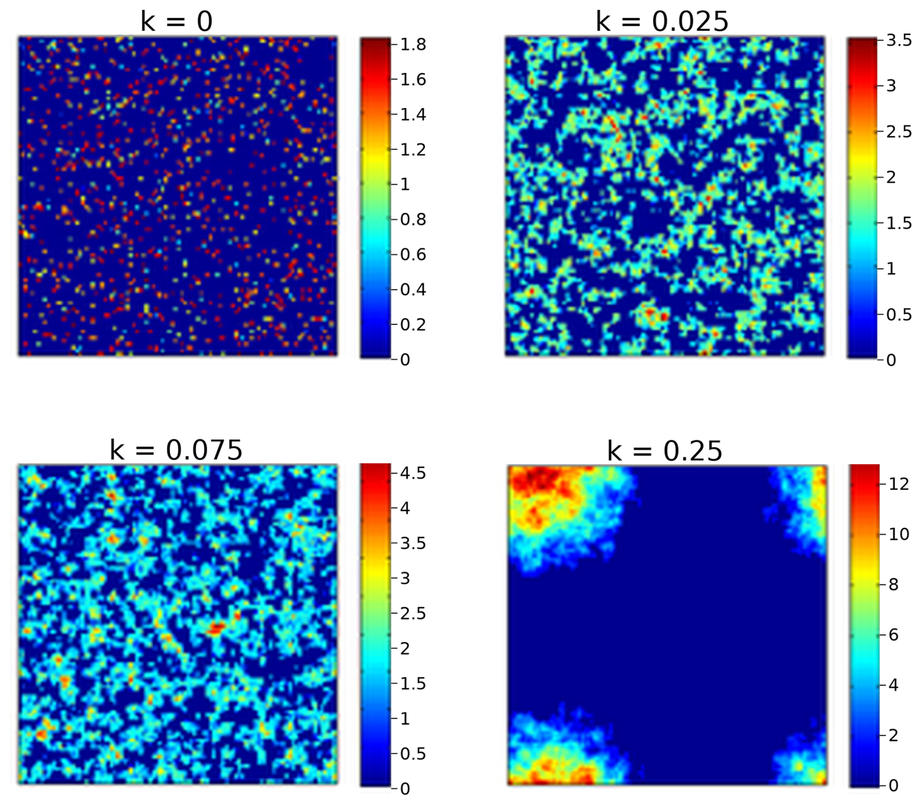
After the steps described in Sect. 2.1–2.3, we analyse the cluster area and rain (based on the constraint we imposed) statistics after each radiative time step t, a snapshot has been shown in Fig. C1 (Appendix C) as an example. The cluster statistics are then used to generate the scaling results in the following.

3 Cluster distributions from CA

3.1 Two-dimensional site percolation

Since CA depends on the two adjustable parameters, γ and d, we denote CA with the coupling constant γ, driven with a magnitude d, as CA_γ,d for brevity. For example, CA_0,d has the meaning of the CA with γ = 0, and with an instability of magnitude d added to each lattice sites at each driving cycle (Eq. 1).

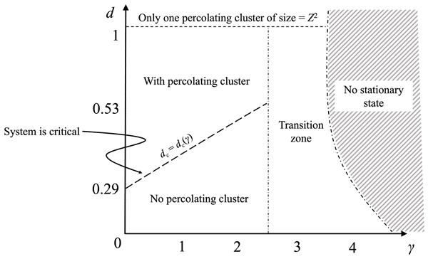
The phase space for CA as a function of γ and d is represented schematically in Fig. 3. For 0 ≤ γ ≤ 2.5, the cluster distributions are found to follow the scaling ansatz similar in form to the 2-dimensional site-percolation (e.g., Christensen and Moloney, 2005) when d approaches a critical value (d_c):

$$\begin{array}{}\text{(7)}& f_{\mathrm{S}}\left(s\right)\propto \left\{\begin{array}{ll}{s}^{-{\mathit{\zeta }}_{\mathrm{S}}}{\mathcal{G}}_{\mathrm{S}}\left(\frac{s}{{\mathit{\xi }}_{\mathrm{S}}^{D_{\mathrm{S}}}}\right)& d\to d_{\mathrm{c}},a\gg \mathrm{1},Z\gg {\mathit{\xi }}_{\mathrm{A}}\\ s^{-{\mathit{\zeta }}_{\mathrm{S}}}{\stackrel{\mathrm{̃}}{\mathcal{G}}}_{\mathrm{S}}\left({\displaystyle \frac{s}{Z^{D_{\mathrm{S}}}}}\right)& d\to d_{\mathrm{c}},a\gg \mathrm{1},\mathrm{1}\ll Z\ll {\mathit{\xi }}_{\mathrm{A}}\end{array}\right.\end{array}$$

where f_S(S) is the discrete probability distribution P(a) when S is A and f_S(s) is the probability density function, f(r), when S is R; 𝒢_S(x) and ${\stackrel{\mathrm{̃}}{\mathcal{G}}}_{\mathrm{S}}\left(x\right)$ are the scaling functions for the two different ξ_A regimes, but share the same generic property of approaching to some non-zero constants when x ≪ 1 and decays rapidly when x ≫ 1; ξ_S is the characteristic “length scale” of the cluster and the D_S is a γ-dependent exponent for the distributions; d_c a γ-dependent value of d where the CA is critical when d = d_c; Z is the lattice size. When S is A, ξ_A has the meaning of a geometric length scale of the cluster (e.g., the averaged radius of gyration of the clusters; Cheraghalizadeh et al., 2024) and based on which separating the two scaling regimes in Eq. (7); D_A, the cluster fractal dimension and ${\mathit{\xi }}_{\mathrm{A}}^{D_{\mathrm{A}}}$, the characteristic cluster area. Similarly, ${\mathit{\xi }}_{\mathrm{R}}^{D_{\mathrm{R}}}$ is the characteristic cluster total rain rate.

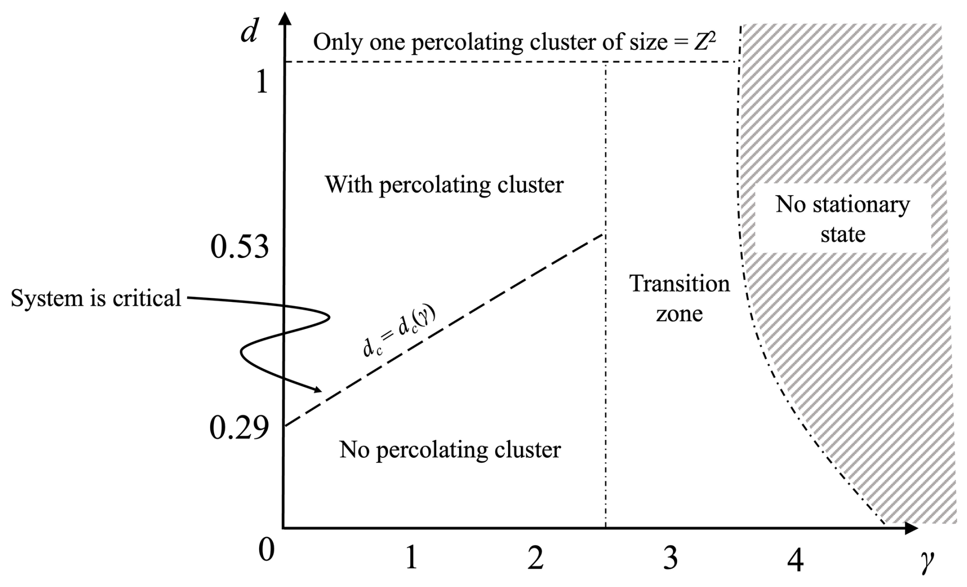
Figure 3 Schematic representation of the phase space of CA as a function of the drive magnitude d and the coupling constant γ. The dash line indicates the critical drive magnitude d_c that is γ-dependent, a state when percolating cluster emerges and the characteristics scale diverges. For infinite-size domain, distribution is pure power law. When d → $d_{\mathrm{c}}^{+}$, distribution is finite scaling whose characteristic scale depends on the domain size. The percolating cluster is more filling with increasing d and increasing separation of scales. When d → ${}_{\mathrm{c}}^{-}$ (no percolation cluster), distribution is finite scaling whose characteristic scale depends on d − d_c. When γ becomes large, there is a transition zone when the system takes too long computational resource to reach stationarity or stationary period is too short to collect sufficient data for reliable characterization.

Furthermore, the characteristic scale scales as

$$\begin{array}{}\text{(8)}& {\mathit{\xi }}_{\mathrm{S}}^{D_{\mathrm{S}}}\propto {\left|d-d_{\mathrm{c}}\right|}^{-{\mathit{\eta }}_{\mathrm{S}}},S=\mathit{\{}A,R\mathit{\}},\end{array}$$

where η_S is a γ-dependent exponent.

3.2 Non-interacting lattice

The motivation of the CA scaling ansatz can be most easily inferred from the case when γ = 0. For CA_0,d, there is no interaction amongst the lattice sites; whether a site become unstable (X > 0) after adding d units during its driving phase, depends only on its antecedent value of X. In its stationary state, the probability that a lattice site becomes unstable after being driven is equal to the ensemble mean of the fractional area coverage of the rain clusters, Ω. Hence CA_0,d can be mapped to the 2-dimensional site percolation on a square lattice of the same length, Z, with the probability of occupancy probability, p = Ω(d). This claim is supported by Fig. 4 where the cluster size distributions for CA_0,d being practically indistinguishable from the sample cluster size distributions of a 2-dimensional site-percolation with the estimated Ω of the CA_0,d chosen as p. For Fig. 4b, the drive d for the CA_0,d is set to approximately its critical value such that $\mathrm{\Omega }(d=d_{\mathrm{c}}=\mathrm{0.2901})$ ≈ p_c = 0.5928. This value of d_c is determined from preliminary experiments based on a Z = 128 lattice.

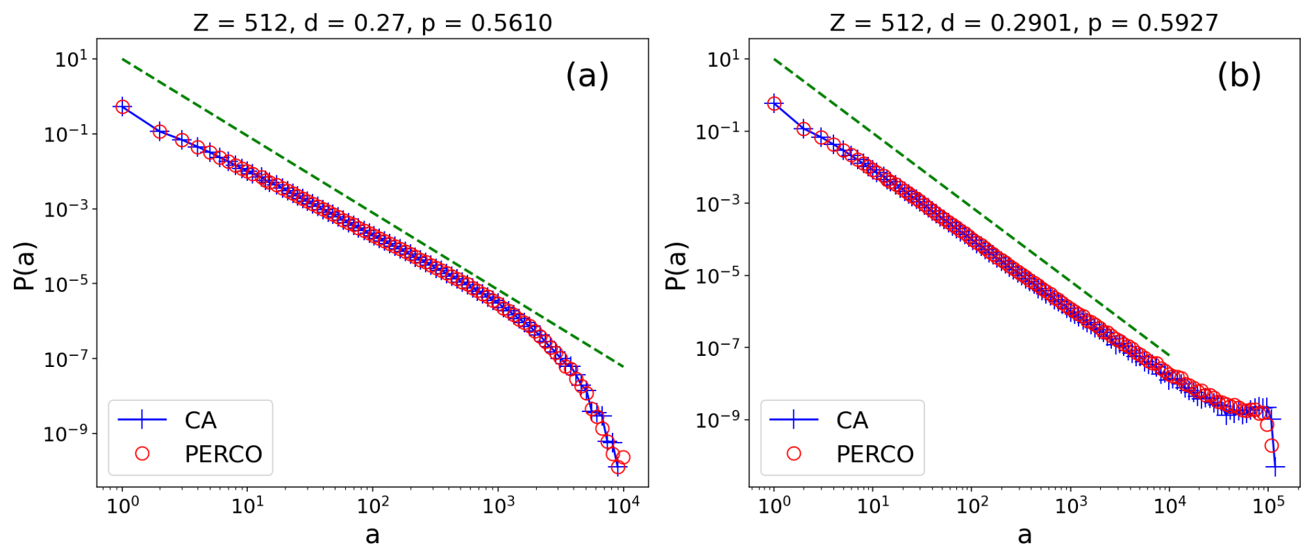
Figure 4 Probability distributions of the cluster size (cross) for CA_0,0.27 (a) and CA_0,0.2901 (b) for Z = 512, together with the cluster size distributions from a 2-dimensional site percolation on a square lattice (open circle) of the same size with occupancy probability p set to the mean averaged fractional rain cluster coverage, Ω, for the CA. Approximately 10⁷ clusters are used to sample the probability distributions. The reference line (green) has slope 187/91.

For the standard site-percolation with occupancy probability p = p_c, the system becomes critical, and the characteristic cluster length scale, ξ_A, diverges. At criticality the system transit to percolation, that is, an incipient infinitely large cluster emerges in the limit of an infinitely large domain, and P(a) ∝ $a^{-{\mathit{\zeta }}_{\mathrm{A}}}$ for a ≫ 1, with ζ_A = 187/91. For standard site-percolation, the characteristic cluster area, ${\mathit{\xi }}_{\mathrm{A}}^{D_{\mathrm{A}}}$ ∝ ${\left|p-p_{\mathrm{c}}\right|}^{-{\mathit{\eta }}_{\mathrm{A}}}$ with η_A = 91/36 (Stauffer and Aharony, 1994). Since p = Ω(d) for CA_0,d, ${\mathit{\xi }}_{\mathrm{A}}^{D_{\mathrm{A}}}$ ∝ ${\left|\mathrm{\Omega }\left(d\right)-\mathrm{\Omega }\left(d_{\mathrm{c}}\right)\right|}^{-{\mathit{\eta }}_{\mathrm{A}}}$ ≈ ${\left({\mathrm{\Omega }}^{\prime }\left(d_{\mathrm{c}}\right)\right)}^{-{\mathit{\eta }}_{\mathrm{A}}}{\left|d-d_{\mathrm{c}}\right|}^{-{\mathit{\eta }}_{\mathrm{A}}}$ to a first approximation, Ω^′(d_c) (> 0) being the first order derivative of Ω evaluated at d_c. On the other hand, when Z ≪ ξ_A, the distribution is finite-size scaling and the characteristic cluster area becomes proportional to $Z^{D_{\mathrm{A}}}$ instead. We will call the scaling ansatz when Z ≫ ξ_A simply as finite scaling to differentiate from finite-size scaling ansatz for clarity.

The finite scaling and finite-size scaling of CA_0,d cluster size distributions is demonstrated in Fig. 5. The d values are judiciously selected such that Z ≫ ξ_A(d) (Fig. 3a). As d approaches d_c (∼ 0.2901), ξ_A increases rapidly and consequently the interval of cluster area where P(a) exhibits a power-law form becomes increasingly discernible. On the other hand, ξ_A(d=0.2905) is much larger than Z ≤ 512, and Fig. 3b is suggestive of finite-size scaling of P(a) for Z ≤ 512.

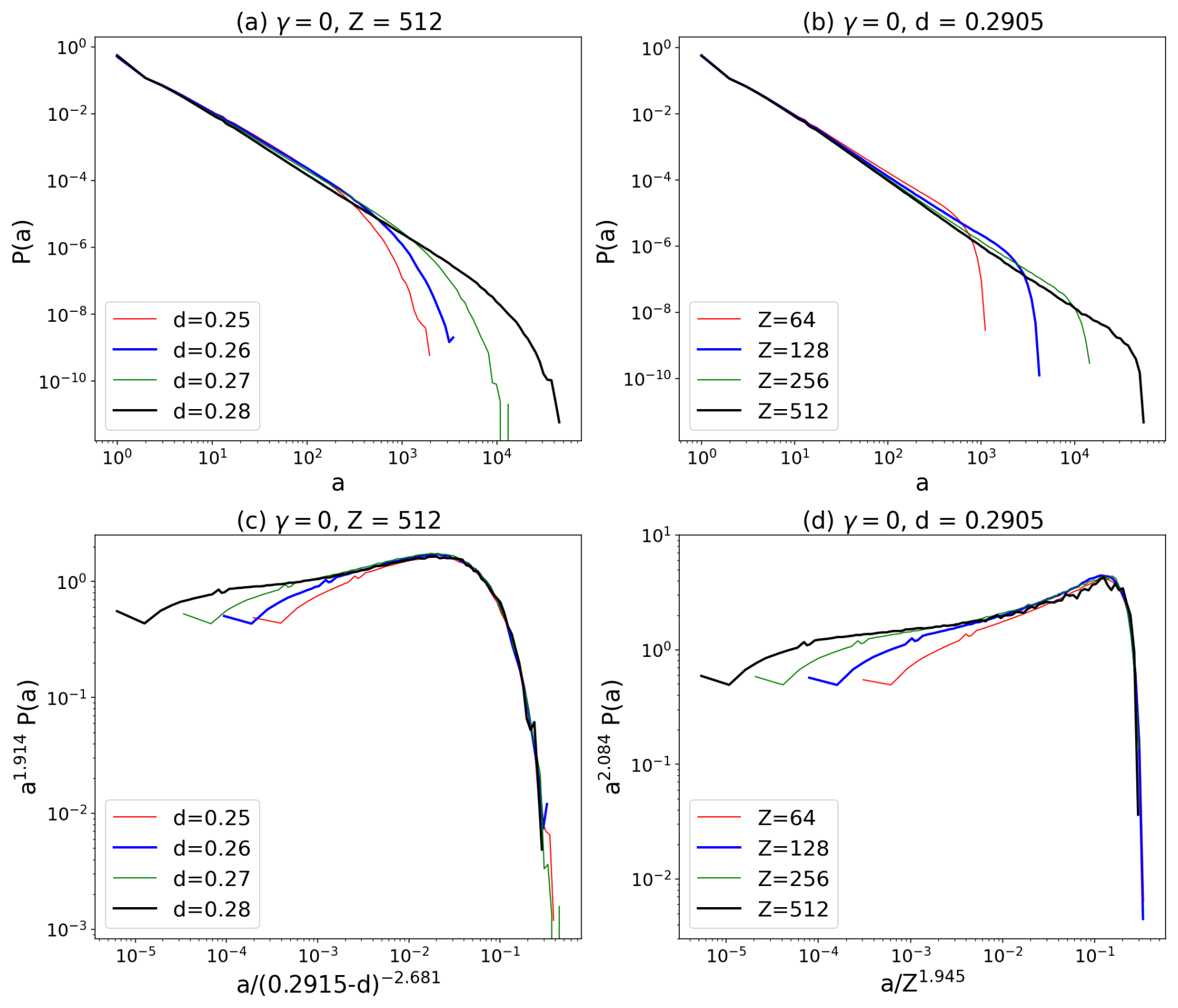
Figure 5 (a) Cluster size distributions for CA_0,d with Z = 512 and d from 0.25 to 0.28 with increment of 0.01 (b) As (a) but with Z = 64, 128, 256 and 512 for CA_0,0.2905. Note that the percolating clusters (largest cluster from each avalanche) are excluded in this case. (c) The data collapse for the distributions shown in panel (a) using estimated values for ζ_A (1.914), η_A (−2.681) and d_c (0.2915) (see main text). (d) Same as (c) but shows the data collapse for the distributions shown in panel (b), with estimated values ζ_A (2.084) and D_A (1.945). Approximately 4 × 10⁷ clusters are used to sample each distribution shown in the plots.

Since the scaling function 𝒢_A (${\stackrel{\mathrm{̃}}{\mathcal{G}}}_{\mathrm{A}}$) is identical in principle, across the different d(Z), the scaling ansatz (Eq. 7) can be tested directly using data collapse, i.e., plotting together the scaling functions inferred separately for the different distributions in Fig. 5a, b. The inferred scaling functions, ${\widehat{\mathcal{G}}}_{\mathrm{A}}$ for the different d values are shown in Fig. 5c, where the reweighted probabilities, $a^{-{\widehat{\mathit{\zeta }}}_{\mathrm{A}}}P\left(a\right)$, are plotted against the x = $a/{\left({\widehat{d}}_{\mathrm{c}}-d\right)}^{-{\widehat{\mathit{\eta }}}_{\mathrm{A}}}$. Note that hatted symbols denote the estimates. The methods used to obtain these estimates are described in Appendix D. ${\widehat{\mathit{\eta }}}_{\mathrm{A}}$ = 2.681 ± 0.067 is slightly larger than the expected theoretical value of 91/36 = 2.528, while ${\widehat{\mathit{\zeta }}}_{\mathrm{A}}$ = 1.914 ± 0.095 is in agreement with the theoretical value of 187/91 ≈ 2.055. The inferred scaling functions associated with the P(a) for the different d values collapse together well for x ≳ 10⁻². For small x (e.g., x ≲ 10⁻⁴ for the ${\widehat{\mathcal{G}}}_{\mathrm{A}}$ with d = 0.28) finite scaling is no longer valid as the cluster distribution would then depends on the details of CA. As d approaches d_c, ξ_A increases rapidly (Eq. 8). Therefore, the lower limit of x where the finite scaling breaks down decreases, evident from the decrease in the x where the overlap of the inferred scaling function beings as d approaches d_c (compare the x where ${\widehat{\mathcal{G}}}_{\mathrm{A}}$ with d = 0.28 collapse with the ${\widehat{\mathcal{G}}}_{\mathrm{A}}$ with d = 0.27, and with d = 0.25 in Fig. 5c). Similar inferences for the scaling function ${\stackrel{\mathrm{̃}}{\mathcal{G}}}_{\mathrm{A}}$ is performed when the distribution is finite-size scaling (Z ≪ ξ_A), with d = 0.2905 as shown in Fig. 3d. Note that as the scaling ansatz in Eq. (7) is defined for finite clusters, the percolating clusters from the numerical simulation are excluded when sampling the clusters. Details of the methods used in estimating D_A and ζ_A are in Appendix D. ${\widehat{D}}_{\mathrm{A}}$ = 1.945 ± 0.057, slightly larger than the theoretical value of 91/48 ≈ 1.896 while ${\widehat{\mathit{\zeta }}}_{\mathrm{A}}$ = 2.084 ± 0.189 agrees with theoretical value of ζ_A.

The scaling characteristics for the CA_0,d cluster total cluster rain rate distributions are similar to that describe above for the cluster size distributions. Figure 6a, b shows the R-distributions when they are finite scaling and finite-size scaling respectively. Away from r ∼ 1, the increasingly discernable power-law form of f(r) for r > 1 when d approaches d_c (Fig. 7a) and with increasing Z (Fig. 7b) are reminiscent to what is observed for P(a). The collapses of the distribution in the two scaling regimes are shown in Fig. 4c, d, using ${\widehat{\mathit{\zeta }}}_{\mathrm{R}}$ = 1.724 ± 0.103, ${\widehat{\mathit{\eta }}}_{\mathrm{R}}$ = 3.742 ± 0.088, ${\widehat{D}}_{\mathrm{R}}$ = 2.596 ± 0.073 and d_c = 0.2925 ± 0.0005 estimated using the same method used in obtaining the exponents for A (see Appendix D). The exponents for R are not independent from those of A due to the constrain E(R|a)αa^β imposed by the CA (Eq. 6 and Appendix A): ζ_A and ζ_R are related with β by the scaling relation (Eq. A4) as a result of the constrain (e.g., Pruessner, 2012). Estimate of β from the scaling relation ${\widehat{\mathit{\zeta }}}_{\mathrm{A}}$ and ${\widehat{\mathit{\zeta }}}_{\mathrm{R}}$ is 1.380 ± 0.338 which is consistent with the imposed value of 4/3. In addition, D_R and D_A area related as follows: The characteristic scale for R ∼ $Z^{D_{\mathrm{R}}}$ which scales as $E\left(R\right|Z^{D_{\mathrm{A}}})$ ∼ $Z^{\mathit{\beta }{D}_{\mathrm{A}}}$. Since the relation is true for all Z (1 ≪ Z ≪ ξ_A), then D_R = βD_A. Similarly, one can demonstrate through Eq. (8) that η_R = βη_A, $\frac{{\widehat{\mathit{\eta }}}_{\mathrm{R}}}{{\widehat{\mathit{\eta }}}_{\mathrm{A}}}$ = 1.3959 ± 0.0675 and $\frac{{\widehat{D}}_{\mathrm{R}}}{{\widehat{D}}_{\mathrm{A}}}$ = 1.3348 ± 0.0763 consistent with the imposed β = 4/3.

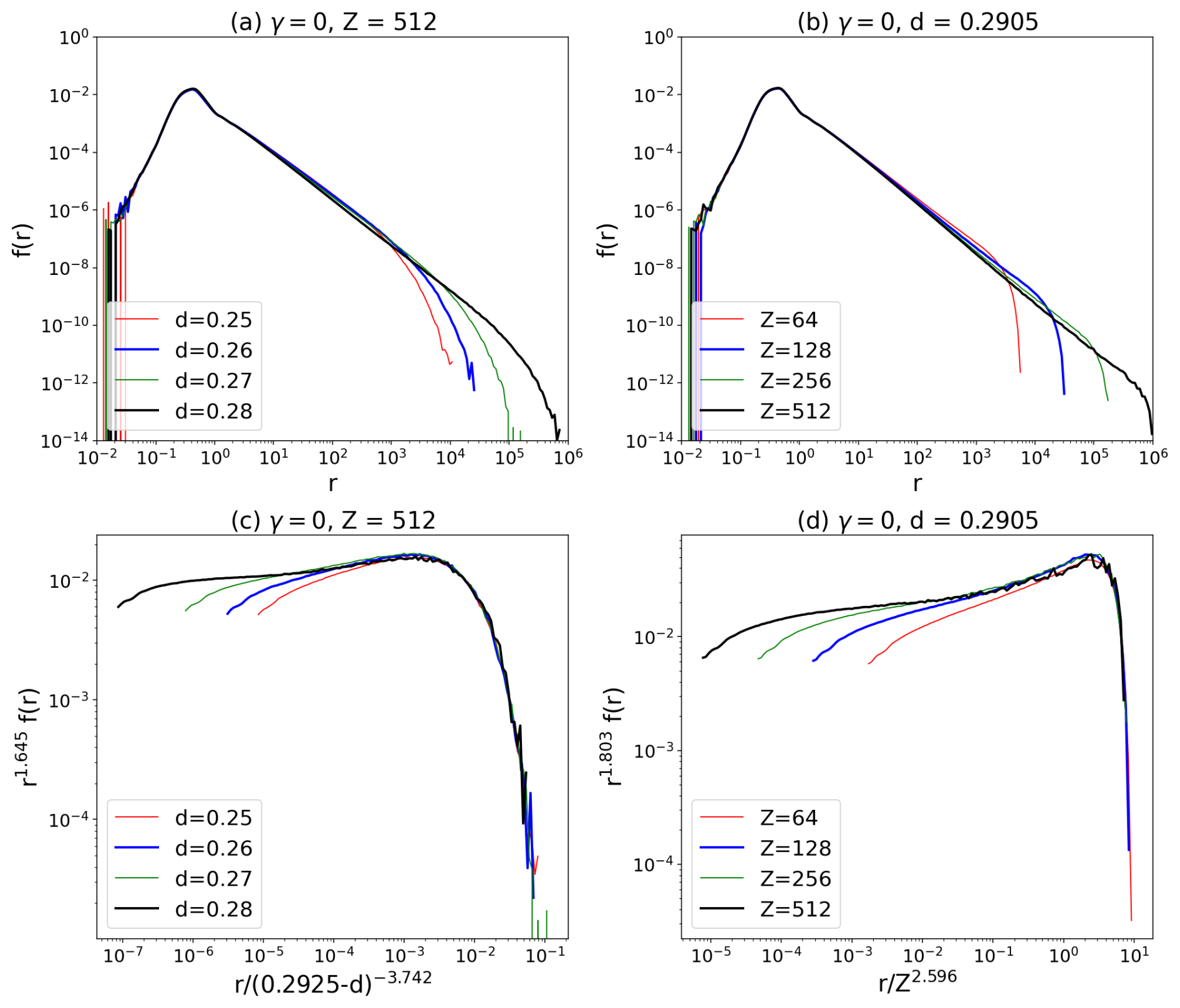
Figure 6 As in Fig. 3 but for the distributions of the cluster total rain rate, with estimated values in (c) ζ_A (1.645), η_A (−3.742) and d_c (0.2925) and in (d) ζ_A (1.803) and D_A (2.596). Note the very small f(r) values for small r in panels (a) and (b), which are due to the single-cell clusters in the model that toppled during simulation and contributed to the pdf.

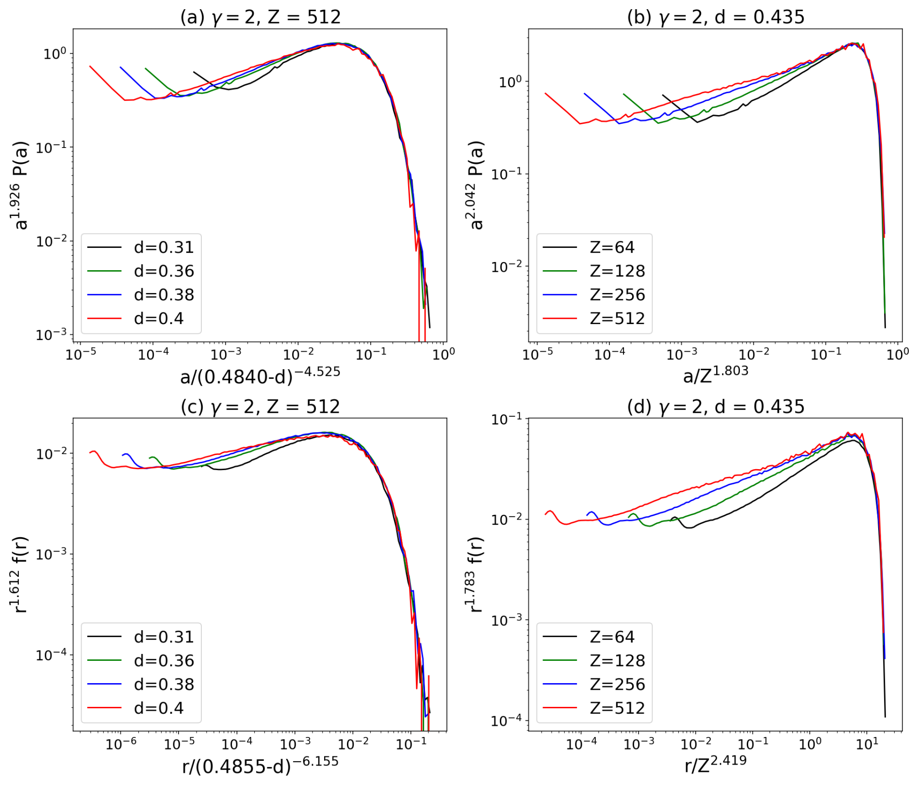
Figure 7 As in Figs. 3c, d and 4c, d but for γ = 2 with d = 0.31, 0.36, 0.38 and 0.40 for panels (a) and (c), and d = 0.435 for panels (b) and (d). The estimated exponents in panels (a) and (c) are ζ_A (1.926/1.612), η_A (−4.525/−6.155) and d_c (0.484/0.4855) respectively, and in panels (b) and (d) are ζ_A (2.042/1.783) and D_A (1.803/2.419) respectively.

In qualitative terms, the non-interacting case (γ = 0) serves as a baseline for understanding the CA's behaviour. Here, each lattice site topples independently of its neighbours, and the only source of spatial organization is the geometric connectivity of toppled sites at quiescence. The fact that the cluster size distribution for CA_0,d is essentially indistinguishable from that of standard 2D site percolation demonstrates that this CA's toppling dynamics naturally generates a percolation-like critical state when the external drive d is tuned to a critical value. In this state, clusters of all sizes emerge, with the largest clusters becoming increasingly space-filling as d approaches d_c. The power-law exponent ζ_A (for cluster area) matches the theoretical percolation value, confirming that the CA's connectivity rule (nearest-neighbour links between toppled sites) is sufficient to reproduce the universal cluster geometry of 2D percolation. This baseline case also establishes that the separation between slow driving and fast relaxation timescales is already sufficient to produce scale-invariant cluster statistics, even before introducing convective interactions.

3.3 Interacting lattice

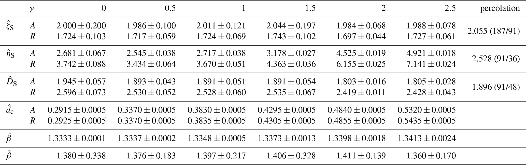
The finite scaling ansatz holds as well for the distributions of CA${}_{\mathit{\gamma },d\to d_{\mathrm{c}}}$ for 0 < γ ≤ 2.5, albeit the following generalizations from CA${}_{\mathrm{0},d\to d_{\mathrm{c}}}$ (Fig. 8 and Table 2): (1) d_c and η_S are increasing functions of γ; (2) D_S is a decreasing function of γ. The method of obtaining the scaling exponents and d_c for each of γ tested are the same as the preceding discussion on CA_0,d (Appendix D). For example, Fig. 7c and d show reasonable data collapse for the two finite scaling regimes Z ≫ ξ_A and 1 ≪ Z ≪ ξ_A for CA_γ,d for the case when γ = 2, using estimates of ζ_S, η_S and D_S and d_c. Similar data collapse with their corresponding scaling exponents estimates are also obtained for γ = 0.5, 1, 1.5 and 2.5 (not shown).

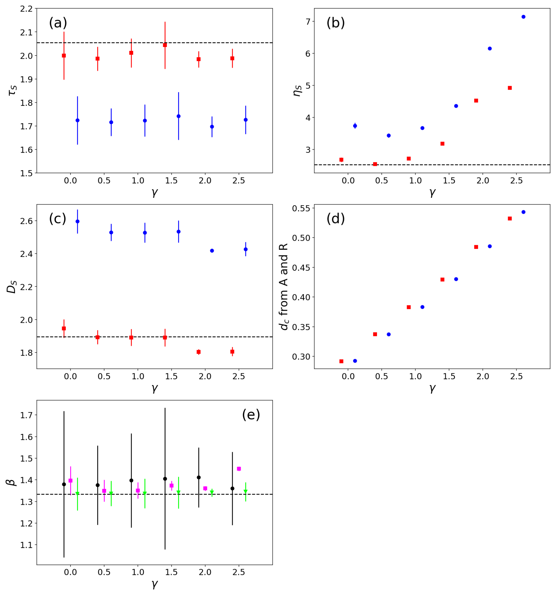
Figure 8 (a–d) Plots of the various estimated scaling exponents and d_c in Table 1 for the distribution for A (red) and R (blue). The dashed horizontal lines are the corresponding values from 2-dimensional site-percolation. (e) β estimated from the scaling relation (Eq. A4; black circle), $\frac{{\widehat{\mathit{\eta }}}_{\mathrm{R}}}{{\widehat{\mathit{\eta }}}_{\mathrm{A}}}$ (magenta square); $\frac{{\widehat{D}}_{\mathrm{R}}}{{\widehat{D}}_{\mathrm{A}}}$ (lime inverted triangle). Dash line is the expected β = 4/3.

Table 2 Numerical estimates of the various scaling exponents and critical values for the A and R distributions for the CA. The corresponding theoretical scaling exponents for the 2-dimensional site-percolation are listed in the last column for reference. The last row is the expected β from the scaling relation (Eq. A4).

d_c increases with γ since the net instability being removed by a convection event (toppling) depends linearly on γ. Hence as γ increase, the magnitude of d needed to drive the model to criticality increases linearly as well (Fig. 8d). D_A is a decreasing function of γ since the suppression of convection by GW1 becomes stronger with increasing γ. Hence, we might expect that the CA rain clusters to be increasingly riddled with “holes” and consequently, their fractal dimension which D_A represents decreases. As expected, D_R and η_R appears to be simply an amplification of D_A and η_A respectively, since the imposed scaling of E(R|a) in the CA constrains the ratio of $D_{\mathrm{R}}/D_{\mathrm{A}}$ and ${\mathit{\eta }}_{\mathrm{R}}/{\mathit{\eta }}_{\mathrm{A}}$ to be β. Figure 8e shows that the expected relation is well reproduced in the CA for D_R and D_A, but not as well for γ ≥ 1.5 for η_R and η_A. The estimates of ζ_A, ζ_R and β for the CA also satisfy the scaling relation Eq. (A4) for all γ tested.

In contrast with η_S and D_S, ζ_S appear to be insensitive to γ for γ ≤ 2.5, with an average value of 2.003 ± 0.058 for ${\widehat{\mathit{\zeta }}}_{\mathrm{A}}$, which agrees with the exponent for percolation (187/91) and 1.721 ± 0.067 for ${\widehat{\mathit{\zeta }}}_{\mathrm{R}}$. Whether the true ζ_A for the CA is identical to that of the 2-dimensional site-percolation (187/91) when γ > 0 remains to be explained. The site interactions due to the gravity waves would have introduced a degree of spatial correlation of X over the domain and hence, CA${}_{\mathit{\gamma }>\mathrm{0},d}$ would not have a one-to-one correspondence with the 2-dimensional site-percolation, as evident from the deviations of ${\widehat{\mathit{\eta }}}_{\mathrm{A}}$ and ${\widehat{D}}_{\mathrm{A}}$ from the percolation values with increasing γ. On the other hand, ${\widehat{\mathit{\zeta }}}_{\mathrm{A}}$ for γ > 0 are the same across within their error estimates from our analysis (Table 2 and Fig. 6a). Although ${\widehat{\mathit{\zeta }}}_{\mathrm{A}}$ for γ = 0.5, 2 and 2.5 is significantly different from the expected value for 2-dimensional percolation of 187/91, we note that for γ = 0, the point estimate for ζ_A is ∼ 0.055 less than 187/91 as well. The possible reason behind the discrepancy could be that although care has been taken in allowing a fairly large range of ξ_A and Z to probe the scaling functions in our present analysis, the number of clusters used (𝒪(10⁷)) to probe scaling function for the larger domain sizes (Z = 128, 512) may still be insufficient, and contributes to the biases in the point estimates. The value of 187/91 would be within the prediction interval of all the ${\widehat{\mathit{\zeta }}}_{\mathrm{A}}$ for γ > 0 if adjusted for similar magnitude of underestimates.

As d increases towards unity beyond d_c, the percolating cluster becomes increasingly space-filling. Since the finite clusters can only exist in the gaps of the percolating cluster, the sizes of the finite clusters decrease rapidly with the increasing d. Consequently, on a probability plot such as those shown in Fig. 9, the frequency of clusters of size in the order of the domain size increases rapidly with d, while the characteristic size of the finite clusters decreases rapidly. When Z≫ξ_A(d), as the case for d = 0.42 and 0.6 for γ = 0 and γ = 2 respectively in the figure, there is a clear separation of scales in the cluster size distribution. When d is unity, there is only one trivial (percolating) cluster of a = Z².

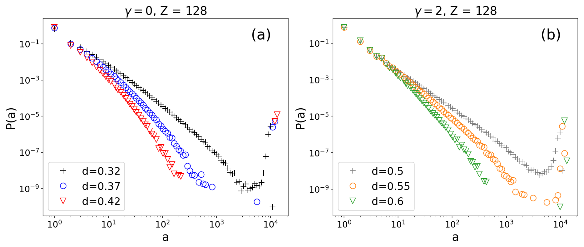
Figure 9 CA sample cluster size distributions for large d values (relative to d_c) using a domain size Z = 128. (a) γ = 0 with d = 0.32 (black crosses), 0.37 (blue circles) and 0.42 (red triangles) (b) γ = 2 with d = 0.50 (gray crosses), 0.55 (orange circles) and 0.60 (lime triangles). About 10⁷ clusters are used to sample each probability distributions.

For increasing γ beyond 2.5, CA takes increasing time to reached stationarity and hence we do not have sufficient sample size to fully characterize the distribution. For γ > 4 the CA the domain averaged instability, X, is found to increase exponentially as the numerical simulation progresses, even with d ≪ 1. The reason behind such a behavior in the CA is because the amount of instability that can be removed at each of the lattice sites behind the GW1 wavefront is constrained by the minimum that X can attain (−1), while X behind the GW2 wavefront (the nearest neighbours of a relaxing site) is not bounded above (Eq. 5). Hence for large enough γ, the total change in X after a toppling can be positive which represents a deep convection rain processes that introduce net instability to the atmosphere instead of stabilizing the atmosphere. As such we regard such model configuration as non-physical and choose not to analyse the model in these large γ regime.

The β estimates analysed from the CA cluster samples (Table 2 and Fig. 9) are close to 4/3 as expected. The procedure of estimating β for each γ tested (γ ∈ $\mathit{\{}\mathrm{0},\mathrm{0.5},\mathrm{1},\mathrm{1.5},\mathrm{2},\mathrm{2.5}\mathit{\}}$) is similar to that carried out for in T21. The only difference from T21 is that for the CA, b in the Eq. (2) is modelled as a linear function of 1/Z, following T17, as shown in Fig. 10a using the case when γ = 2 by way of an example. From Fig. 10b, β appears to be an increasing function of γ. This is because with increasing γ, the occurrence of multiple toppling at a given lattice site may have increased for larger clusters resulting in a slight dependence of the avalanche intensity with the cluster area.

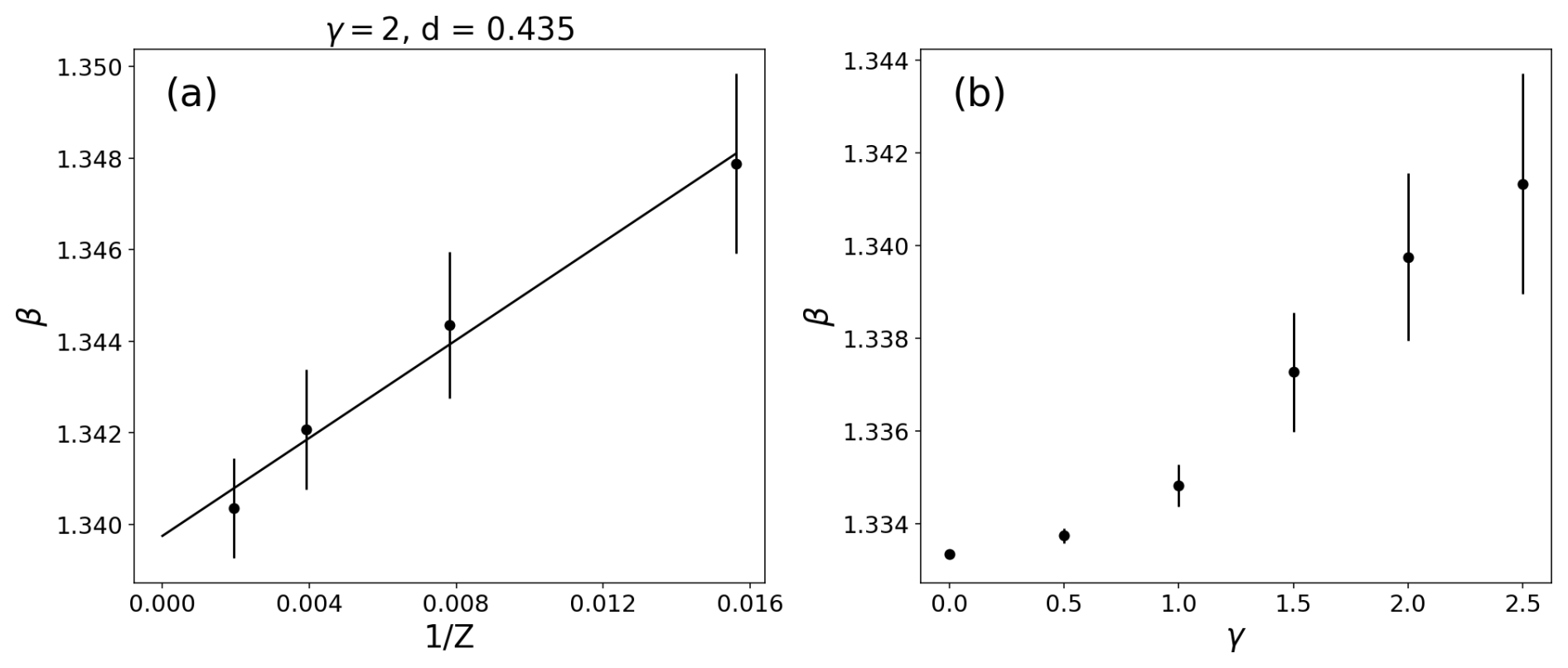
Figure 10 Estimates of β for the CA. (a) The linear regression model to estimate β for CA_2,0.4532 using the various $\mathit{\beta }(\mathrm{1}/Z)$ (Eq. A3), where the regression intercept is taken as $\widehat{\mathit{\beta }}$. (b) Estimated β as a function of γ. The error bars in both plots are the 95 % confidence interval of the regression estimates.

Physically, the interacting case (γ > 0) introduces convective coupling between neighbouring sites through the stabilizing and destabilizing effects of gravity waves (GW1 and GW2). As γ increases, the spatial correlations in the instability field X become stronger: the destabilizing GW2 encourages convective triggering in the immediate vicinity of an existing event, while the stabilizing GW1 suppresses convection further away. This leads to two notable qualitative changes in the cluster statistics. First, the fractal dimension D_A decreases with γ; clusters become more ramified and hole-ridden because the stabilizing far-field influence inhibits the filling of gaps within clusters. Second, the exponent η_A, which governs how rapidly cluster sizes grow as d approaches d_c, increases with γ; the clusters become more sensitive to the precise tuning of the external drive.

Remarkably, despite these changes in the geometric details of the clusters, the exponent ζ_A remains robust to variations in γ, staying close to the 2D percolation value. This robustness suggests that ζ_A is governed by a topological constraint that is independent of the microscopic interaction rules: as long as clusters are defined by nearest-neighbour connectivity on a 2D lattice at criticality, the asymptotic power-law decay of the cluster size distribution falls into the percolation universality class. In contrast, the exponents describing the approach to criticality (η_S) and the geometric structure of clusters (D_S) are sensitive to the details of the interactions, in other words they encode the “fingerprint” of how convection couples neighbouring sites. Thus, this CA provides a clear causal attribution: gravity-wave-mediated interactions shape the spatial structure and correlation length of rain clusters, but they do not alter the fundamental 2D percolation geometry that governs the asymptotic cluster size distribution.

4 Discussions

4.1 A simplified CA

Although the CA exhibits criticality, the ζ_A is different from the observed value of about 5/3 reported in T17. From the results in the preceding section, adjusting the value of γ does not change the ζ_A, although the other critical exponents, η_A and D_A changes with γ. The robustness of the ζ_A lies perhaps more in the dynamics represented by the toppling mechanism in the CA; If we assume that only the destabilization in the vicinity of deep convection by GW2 is the main mechanism behind the rain clusters organization, the CA can be further simplified by excluding the effects of stabilization of the atmosphere by GW1 in Eq. (5). Following the discussion in Sect. 2, the dissipative coefficient, ϵ, for this simplified CA, call it sCA, would be ϵ = $\mathrm{1}-\frac{\mathrm{3}}{\mathrm{4}}\mathit{\gamma }$. By the ASM (Dickman et al., 1998; Vespignani and Zapperi, 1998), sCA may potentially exhibit SOC if γ → 4/3 (i.e., ϵ → 0) and d → 0⁺. In fact, sCA${}_{\mathit{\gamma },{\mathrm{0}}^{+}}$ (the subscripts having the same meaning as the preceding section) is similar to the OFC earthquake model (in which stress in the lattice sites is analogous to atmospheric instability in our CA and when stress is over a threshold a site topples; Olami et al., 1992), in terms of its rules for nearest-neighbour interactions, γ as a control of the level of non-conservation (i.e., not all toppling energy passes to neighbours), as well as how the model is driven. The OFC model is widely accepted to be an SOC when bulk conservation is enforced (i.e., dissipation ϵ = 0; Bröker and Grassberger, 1997; Chabanol and Hakim, 1997; De Carvalho and Prado, 2000). Indeed, preliminary survey with a set of small domain experiments indicates that sCA${}_{\mathrm{4}/\mathrm{3},{\mathrm{0}}^{+}}$ is a SOC (Fig. 11), with ζ_A ≈ 1.35. We use the bulk driving scheme of the OFC model (Olami et al., 1992) to achieve the vanishing drive (d → 0⁺) for this set of experiment. When γ = 0, sCA_0,d also exhibits critically at d = d_c ≈ 0.292 with ζ_A = 187/91 since it is equivalent to CA_0,d whose cluster size distribution is in turn, equivalent to the cluster size distribution of the 2-dimensional site-percolation. The behaviour of sCA${}_{\mathrm{4}/\mathrm{3},{\mathrm{0}}^{+}}$ and sCA_0,d lead us to suspect that in general, for any γ ∈ (0, 4/3), there exist a d = d_c(γ) where sCA${}_{\mathit{\gamma },d_{\mathrm{c}}}$ exhibits criticality, and unlike the case for the CA, ζ_A could be a function of γ as well. We represent our hypothesis in Fig. 9c. Note that ϵ < 0 for γ > 4/3 and hence sCA cannot achieve statistical stationarity for γ > 4/3. We feel that the sCA is a cell-automata which may exhibit critical phenomena, and at the same time “tunable” via γ to reproduce the observed ζ_A ∼ 5/3. Indeed, some finitely driven cellular automata are reported to display varying power-law exponents in their event size distributions (Piegari et al., 2006).

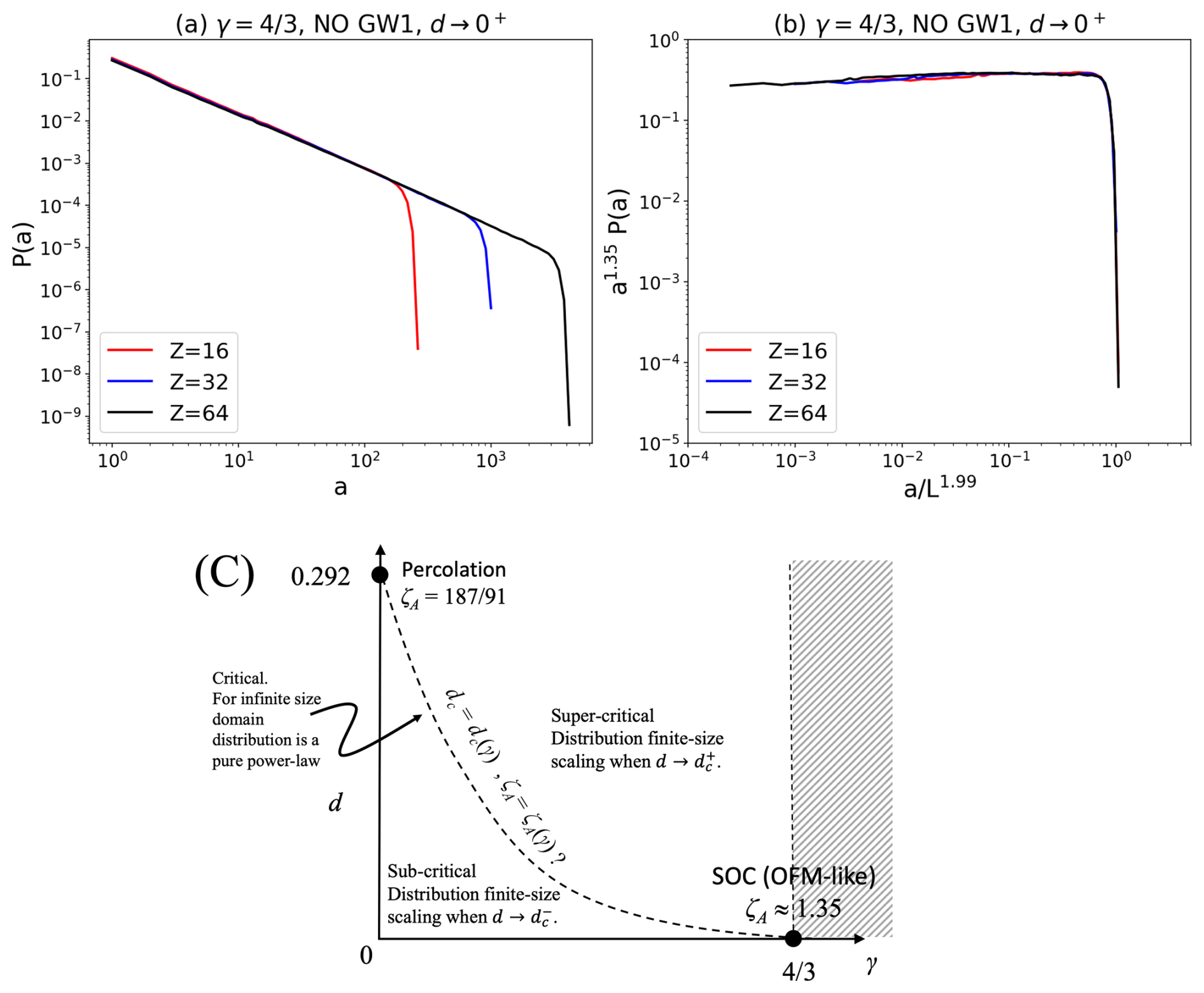
Figure 11 Characteristics of the sCA (CA excluding the representation of the GW1 dynamics in its toppling mechanisms). (a) The distribution of cluster area for different domain size (Z = 16, 32, 64) and (b) its data collapse for the sCA with γ = 4/3 and with d → 0⁺. (c) Schematic illustrating the hypothetical phase space of the sCA_γ,d. The curve d = d_c(γ) represents the unknown critical line of the sCA. sCA is unphysical beyond γ = 4/3 (stippled area).

4.2 Modelled rain clusters

Interestingly the ζ_A estimates from the clusters simulated by a tropical-band model in T21 over Indian Ocean and Atlantic Ocean are close to that of the CA clusters (cf. Table 1 of T21 and Table 1 here) which suggests that the modelled rain clusters may behave like percolating clusters, at least over the Indian Ocean and tropical Atlantic. Peters et al. (2009) analysis of observed rain clusters suggests a ζ_A close to the percolation value as well. However, more effort is needed to elucidate the reasons behind the discrepancy between the ζ_A estimates from observation reported by T17 and Peters et al. (2009) to ascertain which value is more representative of the actual exponent.

The distributions of the modelled rain cluster size, for example by regional climate model (RCM) in T21, for all tropical oceanic regions that include the spanning clusters in the data samples show a “bump” at the large cluster sizes (see Fig. 2 of T21). This is reminiscent of the CA in the supercritical region, where a domain-spanning cluster emerges. In the atmospheric context, such a spanning cluster should not be interpreted literally as a continuous precipitating entity, but rather as a large-scale, connected region of active convection (e.g., the ITCZ or a monsoon trough), within which individual convective cells are dynamically linked. The “bump” in the RCM distributions may therefore reflect the model's tendency to produce overly persistent and spatially extended convective organization compared to observations.

4.3 Physical interpretation of the scaling exponents

The construction method and results from our CA model have implications to some recent studies on tropical rain clusters statistics. While Haerter (2019) focused on cold-pool dynamics of convective self-aggregation, the stochastic model they constructed simulated the effect of gravity currents away from the centre of precipitation cell with scale ∼ 10–100 km, similar to the action of GW1 and GW2 in our model. However, cluster size statistics have not been explored in Haerter (2019). On the other hand, analysis of a range of dynamical models (from general circulation model to RCE models with different model settings) in Stephan and Stevens (2025) showed that large-scale vertical overturning (i.e., planetary and synoptic scale variability) is critical for rain cluster size statistics to follow power law. This might be related to the larger ζ_A over the Pacific Ocean compared with other oceanic regions obtained in T21. While such large-scale variability has not been represented in our CA model, our lattice cell interactions through GW1 and GW2 have provided an answer to one of the discussion questions raised by Stephan and Stevens (2025), namely, “Is there an important feedback from convection, i.e., is the generation of waves and vertical motions by condensation relevant for the relationship between atmospheric motions and the distribution of column water vapor?

Nevertheless, we have imposed the scaling relationship between cluster rain rate and size in our CA model (via β in Eq. 6). T21 has argued that β may be a more fundamental parameter than the individual scaling exponents for cluster rain and area (i.e., ζ_R and ζ_A) as β can be estimated through some fundamental mesoscale dynamical processes (convective heating, entrainment, updraught velocity). With only gravity wave effects implemented in our model, indeed we have obtained robustness of the ζ_R and ζ_A exponents under different coupling strength γ. Such robustness warrants further physical interpretation. The parameter γ controls the strength of gravity-wave-mediated coupling between convective sites. This leads to stronger spatial correlations in the instability field X, which manifests in the critical exponents that describe the spatial structure and correlation length of the clusters: the fractal dimension D_A and η_A possessing sensitivity of the cluster sizes to the proximity of the critical drive. In contrast, ζ_A appears to be governed by a more fundamental topological constraint. The rain clusters defined by nearest-neighbour connectivity of toppled sites form a set of connected components on the lattice. Regardless of the details of the interaction rules that determine which sites topple, as long as the system is driven to a critical point characterized by a divergent correlation length, the cluster size distribution of such connected components falls into the universality class of two-dimensional percolation. In the CA, γ modifies the “microscopic” rules (the interaction strength) but does not change the fundamental fact that the clusters are nearest-neighbour-connected sets on a 2D lattice at a critical point, thus leaving ζ_A unchanged. The other exponents, η_S and D_S, are “non-universal” in the sense that they describe the approach to criticality and the geometric details of the clusters, which are indeed sensitive to the specific interaction rules.

The fact that our simple CA, incorporating only gravity-wave-mediated interactions, yields a ζ_A near the 2-dimensional percolation value (187/91) rather than the observed ∼ 5/3 does not contradict the hypothesis that the observed scaling may depend on only a few fundamental physical constraints. On the contrary, it offers a valuable diagnostic attribution: it demonstrates that gravity wave dynamics alone drive the system towards a percolation universality class, and that reproducing the observed 5/3 exponent likely requires additional fundamental physical ingredients, such as cold-pool dynamics (Haerter, 2019), large-scale vertical overturning (Stephan and Stevens, 2025), or moisture–radiation feedback, that are not yet represented in the current model.

This highlights the distinctive level of explainability offered by reductionist CA models. Because each rule in the CA maps directly to a specific, well-defined physical process, any emergent change in the statistical exponents can be causally traced back to its underlying mechanism. In contrast, high-resolution dynamical models, while more realistic, often convolve numerous interacting processes, making it difficult to isolate which physical ingredient drives a particular statistical behaviour. The CA approach thus serves as a controlled testbed or sandbox for systematically testing which physical mechanisms are necessary and sufficient to reproduce observed rain cluster statistics.

A key direction for future research is to extend the CA framework with simple site coupling mechanism by incorporating additional candidate mechanisms (e.g., cold-pool spreading, horizontal moisture advection, or wind shear) and to examine whether they can shift ζ_A from the percolation value towards the observed 5/3, and whether the crossover behaviour from β = 4/3 to β = 1 in E(R|a) when a MCS grows in size can emerge naturally rather than being imposed. As a side note, Stephan and Stevens (2025) focused on comparing the scaling exponents of CWV “islands” cluster area (i.e., those above a certain water vapor threshold with triggering deep convection consideration) distributions with observations and high-resolution simulations (Li et al., 2022). CA models with CWV as the central ingredient, such as a few those we reviewed in the introduction, may be validated along that line of thought.

5 Summary

A cellular automaton (CA) representing convective organization in a radiative-convective equilibrium is presented. This CA is based only on a limited set of physical processes governing tropical deep convection and their organization. The basic parameter in the model is the MSE difference between the boundary layer and that at upper level, measuring atmospheric instability. The physical processes include large-scale destabilization and convective cell interaction through horizontally propagating gravity waves, thus separating the driving (synoptic) and relaxation (convective) timescale. Both near-field destabilization and far-field stabilization by the propagating gravity waves are represented in the model. Moreover, the CA cluster rain rate is constrained so that the scaling for E(R|a) (expected rain rate conditioned by rain area) is as observed.

It is important to distinguish between two distinct classes of scaling behaviour in the CA: those that are emergent from the dynamics (the cluster area distribution, its fractal dimension and the associated critical exponents) and those that are externally imposed (relationship between cluster rain rate and cluster area). This distinction highlights both the strength and the limitation of the CA approach. The model successfully demonstrates that percolation-like cluster geometries can emerge from relatively simple convective interaction rules, a finding that helps explain the ubiquity of power-law cluster size distributions in observations and models. However, the intensification of rainfall with cluster size, and thus the precise values of ζ_R, requires additional physical processes (e.g., mesoscale updrafts, cold-pool convergence, or organized inflow) that are not yet represented in the current CA. Future extensions of the model should aim to make the β exponent an emergent property rather than an imposed constraint.

For a broad range of an adjustable model parameter, γ, that controls the degree of stabilization and destabilization in the vicinity of a deep convection, the CA exhibits criticality which is similar to a 2-dimensional percolation, under a critical value of large-scale destabilization of the atmosphere. The ζ_A and ζ_R in the CA are insensitive to the value of γ, estimated to be 2.003 ± 0.058 and 1.721 ± 0.067 respectively. The CA ζ_A is near the value expected for 2-dimensional site-percolation. The observed scaling relation between β, ζ_A and ζ_R (Eq. 3) is reproduced.

Modelled rain clusters such as those in RCM resemble the CA rain clusters in a supercritical state, suggesting that the basin-wide rain clusters from the RCM may behave analogously to the incipient infinite percolating clusters of the CA. Physically, this analogy implies that the RCM produces large-scale convective organization (e.g., unrealistic persistent ITCZ-like bands) that spans the model domain. Such behaviour is not observed in nature, where tropical convection is more fragmented and transient. This comparison thus highlights a model deficiency: the RCM's dynamics may overly favour the formation of a single, domain-filling convective system, whereas observations suggest a more balanced distribution across cluster sizes, without a dominant spanning cluster.

Despite the other critical exponents of the CA, namely the η_S and D_S, $S\in (A,R\mathit{\}}$, which vary with γ, the robustness of ζ_S to variations in γ means that a cellular automata that can account for the observed ζ_A ≈ 5/3 may be realized, such as by tuning the stabilization/destabilization of the atmosphere by deep convection induced gravity waves and/or incorporating other mechanisms such as cold-pool dynamics, moisture-radiation feedback and vertical wind shear, and has the potential of exhibiting criticality and reproducing the observed ζ_A ≈ 5/3.

Appendix A

T17 and T21 investigated the scaling behavior of tropical oceanic rain clusters using the framework of SOC. The first study (T17) analyzed satellite rainfall observations (TRMM 3B42), while the second (T21) examined output from a Weather, Research and Forecast (WRF)-based regional climate model over the tropical band. Key concepts and scaling exponents are introduced below.

A1 SOC and scaling laws

Under the SOC paradigm, tropical deep convection is hypothesized to self-organize into rain clusters of all sizes, analogous to avalanches in a critical sandpile. For a system at criticality, the probability distributions of cluster observables follow simple scaling:

$$\begin{array}{}\text{(A1)}& f_{\mathrm{S}}\left(s\right)\sim s^{-{\mathit{\zeta }}_{\mathrm{S}}}{\mathcal{G}}_{\mathrm{S}}\left({\displaystyle \frac{s}{s_{\mathrm{c}}}}\right),s>s_{\mathrm{0}};S\in \mathit{\{}A,R\mathit{\}}\end{array}$$

where S denotes either the cluster area A (in units of grid-cell area ΔA) or the total rain rate R (in units of ΔA × 0.01 mm h⁻¹), ζ_S is the scaling exponent, 𝒢_S is a finite-size scaling function, and s_c is an upper cutoff that increases with domain size. The power-law regime holds for s₀ ≪ s ≪ s_c.

A2 Scaling exponents from observations

Using 15 years of TRMM 3B42 data over the Indo-Pacific warm pool and the intertropical convergence zones (ITCZ) of the eastern Pacific and Atlantic, T17 estimated the scaling exponents for A and R after accounting for domain-size dependence. The universal (basin-independent) values were found to be:

$$\begin{array}{}\text{(A2)}& {\mathit{\zeta }}_{\mathrm{A}}=\mathrm{1.66}\pm \mathrm{0.06}\left(\sim \mathrm{5}/\mathrm{3}\right),{\mathit{\zeta }}_{\mathrm{R}}=\mathrm{1.48}\pm \mathrm{0.13}\left(\sim \mathrm{3}/\mathrm{2}\right).\end{array}$$

Furthermore, the conditional mean of the cluster rain rate given its area, E(R|a), exhibited two distinct scaling regimes:

$$\begin{array}{}\text{(A3)}& E\left(R\right|a)\sim \left\{\begin{array}{ll}{a}^{\mathit{\beta }}& a\le \mathit{\alpha }\left(\text{mesoscale clusters}\right)\\ a^{\mathit{\chi }}& a>\mathit{\alpha }\left(\text{larger clusters}\right),\end{array}\right.\end{array}$$

with β = 1.33 ± 0.03 (∼ 4/3), χ = 0.97 ± 0.04 (∼ 1.0), and the crossover area α with associated length scale ∼ 320 km. For mesoscale clusters (β > 1), growth is accompanied by intensification. While for larger clusters (χ ≈ 1), the average rain intensity saturates, suggesting that superclusters grow mainly by aggregation without further intensification. The exponents satisfy the SOC scaling relation:

$$\begin{array}{}\text{(A4)}& \mathit{\beta }={\displaystyle \frac{\left({\mathit{\zeta }}_{\mathrm{A}}-\mathrm{1}\right)}{\left({\mathit{\zeta }}_{\mathrm{R}}-\mathrm{1}\right)}}\end{array}$$

which holds for the observed values.

A3 Scaling exponents from model output

T21 applied an identical methodology to 28 years of WRF model output (36 km resolution) over the same tropical ocean basins. The model rain clusters did not exhibit universality: the estimated ζ_A and ζ_R varied significantly across basins (e.g., ζ_A ranged from 2.12 ± 0.10 over the Indian Ocean to 2.48 ± 0.09 over the western Pacific). Moreover, the model failed to reproduce the crossover in E(R|a). Instead, a single power law E(R|a) ∼ a^β held over the entire range of cluster sizes, with β = 1.36 ± 0.05 (averaged across basins). This value agrees with the observed β for mesoscale clusters, indicating that the model captures the fundamental intensification dynamics of small-to-moderate clusters. However, the absence of the crossover (i.e., β remaining above unity for synoptic-scale clusters) and the unrealistic basin-wide rain bands produced by the model suggest that its large-scale convective organization departs from reality.

Appendix B

The physical basis and parameter estimation details for the CA rules described in Sect. 2 are provided here for interested readers. The CA uses the stability of the tropical atmosphere as a basis for the model variable. A schematic of the profile of the model h and h^* and various definitions have been shown in Fig. 1 to aid the model description. Specifically, we adopt the Arakawa's penetrative convection (Schubert, 2000) for deep convection

$$\begin{array}{}\text{(B1)}& h_{\mathrm{1}}>\left(h_{\mathrm{2},\mathrm{3}}^{*}\right)>h_{\mathrm{2}}\end{array}$$

where h₁, h₂ and h₃ are the density-averaged of the boundary (1000–850 mb), middle (850–450 mb) and upper layer (100–450 mb) tropospheric specific moist static energy. h^* is the density-averaged saturated moist static energy. Note that h₁ = $h_{\mathrm{1}}(x,y,t)$, where (x, y) is the coordinates of a location on the surface and t is the time. Similar functional dependence for the rest of the layer-averaged parameters. From typical vertical profiles of the observed moist static energy found in the literature (e.g., Emanuel, 1994), it is reasonable to assume $h_{\mathrm{3}}^{*}$ ≈ $h_{\mathrm{2}}^{*}\left(>h_{\mathrm{2}}\right)$ which simplifies the condition for deep convection to occur (Eq. B1) to

$$\begin{array}{}\text{(B2)}& X>\mathrm{0}\end{array}$$

where $X\stackrel{\text{def}}{=}{h}_{\mathrm{1}}-h_{\mathrm{3}}^{*}$ is the primary variable of the CA. In the CA, the atmosphere is stable against deep (moist) convection when X < 0 and is defined to be bounded below by say, X₀ (< 0), representing the notion that the atmosphere has a maximum stability attainable. From here on, all variables in the CA having the same units of X is understood to be normalized by $\left|X_{\mathrm{0}}\right|$. Hence X ≥ −1 in the CA.

B1 Large-scale destabilisation (Eq. 1)

We assume that the large scale moist static energy at the boundary layer to be the net result of the radiative fluxes and the latent and sensible heat fluxes at the surface provide the large scale forcing. At the upper troposphere, the moist static energy is assumed to change in response to the net radiative fluxes only. Changes of the moist static energy as a result of large scale vertical and horizontal advection is not considered in the CA. By assuming that the time rate of change of $h_{\mathrm{3}}^{*}$ is the same as the rate of change of h₃,

$$\begin{array}{}\text{(B3)}& {\dot{X}}_{\mathrm{LS}}=F_{\mathrm{1}}+E_{\mathrm{1}}-E_{\mathrm{3}}\end{array}$$

where ${\dot{X}}_{\mathrm{LS}}$ is the large-scale rate of change of X (e.g., the spatial-temporal averages of $\mathrm{d}X/\mathrm{d}t$ across the domain, and over a time interval, t_LS, much longer than the convective timescale); E₁ and E₃ the rate of large-scale heating from radiation at the boundary layer and upper tropospheric layer respectively; F₁ the large-scale heating rate due to the latent and sensible heat fluxes. Typical value for the rhs of Eq. (B3) for the tropical atmosphere estimated from existing literature are as follows: F₁ ≈ 6.774 kJ kg⁻¹ d⁻¹, E₁ ≈ −1012 J kg­⁻¹ d⁻¹ and E₃ ≈ −1006 J kg⁻¹ d⁻¹. Hence ${\dot{X}}_{\mathrm{LS}}$ ≈ 5.768 kJ kg⁻¹ d⁻¹, which means that the large scale forcing drives the tropical atmosphere towards instability. The amount of instability added in the CA at each lattice site, in a large-scale (or outer) time step, is

$$\begin{array}{}\text{(B4)}& d={\dot{X}}_{\mathrm{LS}}{t}_{\mathrm{LS}}>\mathrm{0}\end{array}$$

B2 Local effects of a deep convection process (Eqs. 2–4 in Table 1)

At the site where deep convection occurs, deep convection is assumed to transport the moist static energy from the boundary layer into the upper troposphere, thereby increasing h₃ and $h_{\mathrm{3}}^{*}$ under the simplifying assumption that the upper tropospheric layer is nearly saturated. At the same time, the compensating downdraft transports the low-h air from the mid troposphere into the boundary layer decreasing h₁. Therefore, the deep convection process decreases X at the site where the deep convection happens, stabilising the atmospheric column above the site. The amount of stabilisation

$$\begin{array}{}\text{(B5)}& \mathrm{\Delta }{X}_{\mathrm{c}}\stackrel{\mathrm{def}}{=}{X}_f-X_i\le \mathrm{0}\end{array}$$

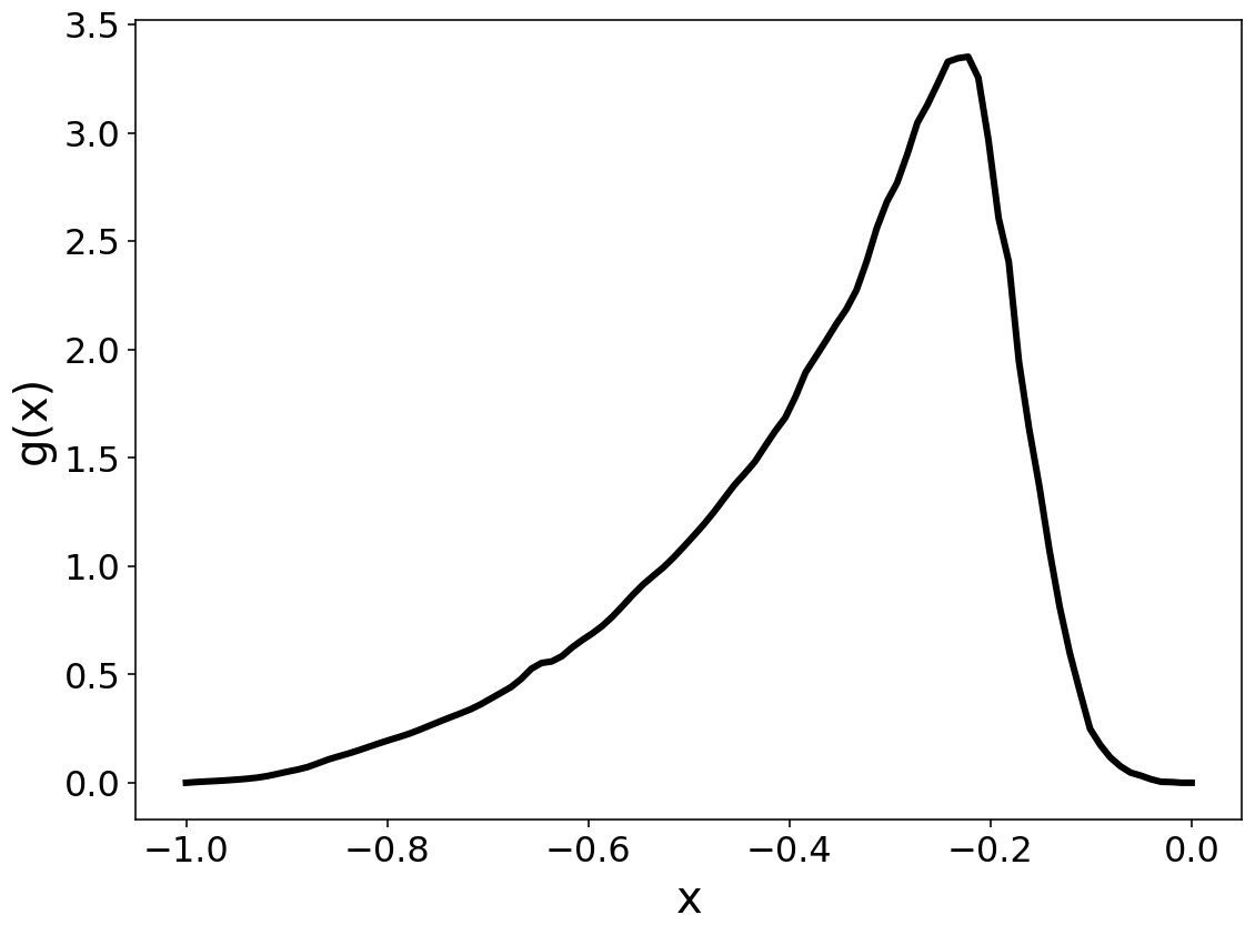
where the i and f subscript denotes before and after convection. In the CA, the value X_f is a random variable with a probability distribution, g(X_f), to reflect the stochasticity in the deep moist convection due to the entrainment and detrainment of cloudy and sub-saturated environmental air that affects how much of the local instability has been removed by the deep convection. The distribution, g(X_f), is shown in Fig. B1. This distribution is estimated as follows: by making a crude assumption that X_f is proportional to the column precipitable water, W, in the column of air after the deep convection, we exploit the observations by Peters and Neelin (2006) by estimating the frequency of non-rainy instances given at different W (the differences between number of occurrences for a given w (rainy and non-rainy) minus the number of occurrences for a given w which are rainy from their Fig. 3).

Figure B1 The distribution for X_f.

B3 Effects of gravity waves excited by deep convection (Eq. 5 in Table 1)

Gravity waves effects have long been recognized as an important mechanism for convection clustering (Randall and Huffman, 1980; Mapes, 1993). The CA assumes that a deep convection event has a top heavy latent heating profile at the convecting site which is a linear combination of two modes of heating profiles, Q₁ and Q₂, with vertical wavenumbers ℓ = 1 and ℓ = 2 (the vertical wavelength is 2$H/\mathrm{\ell }$, H being the scale height of the deep convection). Referring to the schematics in Fig. 2, the horizontal gravity bores radiates outwards from the convecting site with a circular wave front with phase speed of c_ℓ ≈ $NH/\left(\mathrm{\ell }\mathit{\pi }\right)$, N being the buoyancy frequency (Nicholls et al., 1991). In the lifetime of the deep convection, τ_c (≪ τ_LS), the two gravity bores GW1 and GW2 have moved a distance r_ℓ = c_ℓτ_c away from the convective site, with r₁ = 2r₂.

The following assumptions are made (1) the flow is hydrostatic, incompressible and the motions outside the convective core to be adiabatic; (2) the horizontal transport of moist static energies is negligible when compare to the vertical transport of the moist static energies; (3) h ≈ h^* for p > p₂, except near the tropopause, where the vertical velocity drops quickly to zero, h^* is near constant within the upper tropospheric layer (see Fig. 1); (4) the pressure levels defining the boundary and upper tropospheric layers are approximately constant. Then, it can be estimated that the change of stabilisation due to GWℓ at the non-precipitating sites behind the gravity bore's wavefront due to the convection, ΔX_ℓ, is

$$\begin{array}{}\text{(B6)}& \mathrm{\Delta }{X}_{\mathrm{\ell }}=-{\mathit{\omega }}_{\mathrm{\ell }}{\left({\displaystyle \frac{\partial h}{\partial p}}\right)}_{\mathrm{b}}{\mathit{\tau }}_{\mathrm{c}};\mathrm{\ell }=\mathrm{1},\mathrm{2}\end{array}$$

where ω_ℓ is the averaged vertical velocity in pressure coordinates at the top of the boundary layer (p = p₁) due to the GWℓ (ℓ = 1,2) behind its wavefront and ${\left(\frac{\partial h}{\partial p}\right)}_{\mathrm{b}}$ is a representation of the effective vertical gradient of h in the boundary layer. Since ${\left(\frac{\partial h}{\partial p}\right)}_{\mathrm{b}}$ > 0, GW1 stabilizes the atmosphere (i.e. ΔX_ℓ < 0) since ω₁ > 0, while GW2 destabilizes the atmosphere since ω₂ < 0 (see Fig. 2). The destabilizing effects due to the GW2 bore is in line with Mapes (1993) where the combined effects of the two gravity bores can destabilise the atmosphere by decreasing the convective inhibition at the vicinity of a deep convection through boundary layer convergence behind the GW2 bore.

By using incompressibility of the flow and the divergence theorem:

$$\begin{array}{}\text{(B7)}& {\mathit{\omega }}_{\mathrm{\ell }}\approx -{\displaystyle \frac{a_{\mathrm{c}}}{A_{\mathrm{\ell }}}}{\mathit{\omega }}_{\mathrm{c}\mathrm{\ell }}\end{array}$$

where a_c is the area covered by the deep convection, A_ℓ the area outside the convection but behind the GWℓ wavefront, which is the area of an annulus with an inner radius r_c = $\sqrt{a_{\mathrm{c}}/\mathit{\pi }}$ and an outer radius c₁τ_c (see Fig. 2); ω_cℓ the averaged vertical velocity of the deep convection site at the top of the boundary layer (averaged over a_c and time interval 0 ≤ t ≤ τ_c); w_ℓ the averaged vertical velocity due to GWℓ for sites within the annulus area A_ℓ at p = p₁ (averaged over A_ℓ and time interval 0 ≤ t ≤ τ_c). Since $\left|{\mathit{\omega }}_{\mathrm{c}\mathrm{\ell }}\right|$ is proportional to $\left|Q_{\mathrm{\ell }}\right|$ (more rigorously square of vertical velocity is proportional to heating energy) which in turn is assumed to be proportional to $\left|\mathrm{\Delta }{X}_{\mathrm{c}}\right|$, we have (from Eqs. B6 and B7):

$$\begin{array}{}\text{(B8)}& {\displaystyle }\mathrm{\Delta }{X}_{\mathrm{1}}={\mathit{\gamma }}_{\mathrm{1}}\mathrm{\Delta }{X}_{\mathrm{c}};{\mathit{\gamma }}_{\mathrm{1}}>\mathrm{0}\text{(B9)}& {\displaystyle }\mathrm{\Delta }{X}_{\mathrm{2}}=-{\mathit{\gamma }}_{\mathrm{2}}\mathrm{\Delta }{X}_{\mathrm{c}};{\mathit{\gamma }}_{\mathrm{2}}>\mathrm{0}\end{array}$$

where γ₁ and γ₂ are positive constants which are not are not independent since they are related to the relative magnitude between Q₁ and Q₂. By defining the ratio

$$\begin{array}{}\text{(B10)}& \mathit{\alpha }\stackrel{\mathrm{def}}{=}-{\displaystyle \frac{{\mathit{\omega }}_{\mathrm{c}\mathrm{2}}}{{\mathit{\omega }}_{\mathrm{c}\mathrm{1}}}}>\mathrm{0}\end{array}$$

it is easy to show, using Eqs. (B6)–(B9), that

$$\begin{array}{}\text{(B11)}& {\displaystyle \frac{{\mathit{\gamma }}_{\mathrm{2}}}{{\mathit{\gamma }}_{\mathrm{1}}}}={\displaystyle \frac{A_{\mathrm{1}}}{A_{\mathrm{2}}}}\mathit{\alpha }\end{array}$$

We estimate α from literature by first noting that α = $\frac{L_{\mathrm{2}}}{L_{\mathrm{1}}}$, where L₁ and L₂ are the amplitudes of the latent heating profile that excite the GW1 and GW2 assuming that the latent heating is balance by adiabatic ascent. We approximate that the total heating profile from deep convection as a linear combination of two sinusoids:

$$\begin{array}{}\text{(B12)}& Q\left(z\right)=L_{\mathrm{1}}\sin \left({\displaystyle \frac{\mathit{\pi }z}{H}}\right)-L_{\mathrm{2}}\sin \left({\displaystyle \frac{\mathrm{2}\mathit{\pi }z}{H}}\right)\end{array}$$

We use the vertical latent heating profile over the Tropical Western Pacific inferred from satellite cloud data by Jakob and Schumacher (2008) to estimate L₁ and L₂. The two turning points in their inferred profile in their Fig. 4-3 is about (7 km, 1.38 K d⁻¹) and (1 km, −0.13 K d⁻¹), hence substituting the two co-ordinates into Eq. (B12) and taking H = 14 km and obtained a value of 0.75 for α.

In the CA with a square lattice, the sites behind the GW1 and GW2 wavefronts are taken to be nearest-neighbours and the next-nearest-neighbours (12 lattice sites) and the nearest-neighbours respectively (4 sites). Hence in the CA, A₁ = 12a_c and A₂ = 4a_c. From Eq. (B12) we have γ₂ = $\frac{\mathrm{9}}{\mathrm{4}}{\mathit{\gamma }}_{\mathrm{1}}$. For notational convenience, we defined γ = 12γ₁, hence γ₂ = $\frac{\mathrm{3}}{\mathrm{16}}\mathit{\gamma }$.

Appendix C

The following is an example of our model run, which is a snapshot based on the variable X showing the simulated clusters.

Figure C1 Snapshot of model run based on the distribution of variable X.

Appendix D

As we can obtain rain cluster distributions with well separated characteristic cluster length scales using the CA, we are able to probe the finite size scaling through moment analysis and data collapse to obtain the various scaling exponents for the distribution. In our following discussion all hatted symbols denote the estimates from the sample rain cluster distributions.

D1 Estimating ζ_S

When the distribution is finite-size scaling (1 ≪ Z ≪ ξ_A; Eq. 7), the analysis of moments is used to estimate ζ_S, S ∈ {A,R}. It can be shown that finite-size scaling requires the nth moments of S (Pruessner, 2012) to scales as follows:

$$\begin{array}{}\text{(D1)}& 〈S^n〉\propto S_{\mathit{\xi }}^{{\mathit{\sigma }}_n^{\left(S\right)}},n>{\mathit{\zeta }}_{\mathrm{S}}-\mathrm{1}\end{array}$$

where S_ξ is the characteristic scale of S, which is in principle proportional to $Z^{D_{\mathrm{S}}}$, and

$$\begin{array}{}\text{(D2)}& {\mathit{\sigma }}_n^{\left(S\right)}=\mathrm{1}+n-{\mathit{\zeta }}_{\mathrm{S}}\end{array}$$

We estimate S_ξ(Z) by dividing the third moment with the second moment of S for each Z (64, 128, 256, 512). For each n (equals to 2, 3, 4, 5), ${\widehat{\mathit{\sigma }}}_n^{\left(S\right)}$, is first estimated from Eq. (D1) as the gradient of the linear regression of log 〈Sⁿ〉 against log S_ξ. Finally, ${\widehat{\mathit{\zeta }}}_{\mathrm{S}}$ is estimated using another linear regression of ${\widehat{\mathit{\sigma }}}_n^{\left(S\right)}$ against n, following Eq. (D2). The 95 % confidence interval of the intercept estimates is adopted as the error for ${\widehat{\mathit{\zeta }}}_{\mathrm{S}}$.

When ξ_S≪Z, we observe that the resulting point estimates for ζ_S from the moment analysis described above are generally sub-optimal; the data collapse using the ζ_S estimates from moment analysis does not collapse well. Preliminary trial-and-error for a few cases show that better point estimate for ζ_S can result in better data collapse. We suspect that finite domain effects may still be significant when ξ_S≪Z rendering the moment scaling relation of Eq. (D1) accurate only for domain sizes beyond Z = 512. As such we use an objective data collapse method to estimate ζ_S for ξ_S≪Z. This method exploit the fact that in an ideal data collapse, $M_{\mathrm{S}}\left({\mathit{\zeta }}_{\mathrm{S}},d\right)\stackrel{\mathrm{def}}{=}\underset{s}{\max }{s}^{{\mathit{\tau }}_{\mathrm{S}}}{f}_{\mathrm{S}}(s;d)$, where f_S(s;d) is the probability distribution for S when an external drive d is applied on the CA (for a given γ), is identical across all d. The method of the objective data collapse is outlined as follows: for each ${\widehat{\mathit{\zeta }}}_{\mathrm{S}}\in [a,b]$, calculate $M_{\mathrm{S}}\left({\widehat{\mathit{\zeta }}}_{\mathrm{S}},d_j\right)$ for every d_j (e.g., d_j = 0.25, 0.26, 0.27, 0.28 for the CA_0,d; see Fig. 9a in the main text) and then obtain the sample variance from the set $\left\{\ln M_{\mathrm{S}}\left({\widehat{\mathit{\zeta }}}_{\mathrm{S}},d_j\right)|j=\mathrm{1},\mathrm{2},\mathrm{\dots }\right\}$. The ${\widehat{\mathit{\zeta }}}_{\mathrm{S}}$ that gives the minimum sample variance (and hence the best data collapse out of all the exponent tested) is identified as the best estimate for ζ_S. In our work, [a,b] is an interval covering the range of the likely ζ_S.

The error for ${\widehat{\mathit{\zeta }}}_{\mathrm{S}}$ due to the uncertainty in sampling the probability distribution can be shown to be

$$\begin{array}{}\text{(D3)}& \mathit{\delta }{\widehat{\mathit{\zeta }}}_{\mathrm{S}}\approx {\displaystyle \frac{\mathrm{1}}{B}}\sum _{j=\mathrm{1}}^J\left|\ln s_j^{*}-\stackrel{\mathrm{‾}}{\ln s^{*}}\right|\left|\mathit{\delta }{F}_j^{\left(S\right)}\right|\end{array}$$

where ${s_j^{*}}^{{\widehat{\mathit{\zeta }}}_{\mathrm{S}}}{\widehat{f}}_{\mathrm{S}}\left(s_j^{*};d_j\right)=M_{\mathrm{S}}\left({\widehat{\mathit{\zeta }}}_{\mathrm{S}},d_j\right)$; $\stackrel{\mathrm{‾}}{\ln s^{*}}={\sum }_j\ln s_j^{*}/J$; $B={\sum }_{j=\mathrm{1}}^J{\left(\ln s_j^{*}-\stackrel{\mathrm{‾}}{\ln s^{*}}\right)}^{\mathrm{2}}$; $\mathit{\delta }{F}_j^{\left(S\right)}=\ln \left[{\widehat{f}}_{\mathrm{S}}\left(s_j^{*};d_j\right)+\mathit{\delta }{f}_{\mathrm{S}}^{*}\right]-\ln {\widehat{f}}_{\mathrm{S}}\left(s_j^{*};d_j\right)$, $\mathit{\delta }{f}_{\mathrm{S}}^{*}$ being the error of sample probability distribution ${\widehat{f}}_{\mathrm{S}}\left(s_j^{*};d_j\right)$. We estimate $\mathit{\delta }{f}_{\mathrm{S}}^{*}$ as follows: define $p^{*}=P\left(s_{\mathrm{1}}\le S<s_{\mathrm{2}}\right)$ where $I=[s_{\mathrm{1}},s_{\mathrm{2}})$ is the bin interval containing $s_j^{*}$ and note that the number of clusters out of a total of N clusters that would have s falling within I follows a binomial distribution. For large enough N as in our work, the 95 % confidence interval for the estimates for p^* is ${\widehat{p}}^{*}\pm {\mathit{\sigma }}^{*}$, where ${\widehat{p}}^{*}$ is our binomial proportion estimate for p^* and ${\mathit{\sigma }}^{*}=\mathrm{1.96}\sqrt{{\widehat{p}}^{*}\left(\mathrm{1}-{\widehat{p}}^{*}\right)/N}$. $\mathit{\delta }{f}_{\mathrm{S}}^{*}$ is then estimated as ${\mathit{\sigma }}^{*}/∥I∥$ where $∥I∥=|s_{\mathrm{2}}-s_{\mathrm{1}}|$ if S is R, or ∥I∥ is the number of integers containing within the interval I if S is A.

The estimate for ζ_S presented in the main text (Table 2 and Fig. 6a) is the average estimates from the above two different methods.

D2 Estimating D_S, η_S and d_c

When the distribution is finite-size scaling, we obtain D_S as the regression slope of the characteristic scale S₀ against Z (see above) and the 95 % confidence interval of the regression slope taken as the error of D_S.

When ξ_S≪Z, $S_{\mathrm{0}}\propto {\left|d-d_{\mathrm{c}}\left(\mathit{\gamma }\right)\right|}^{-{\mathit{\eta }}_{\mathrm{S}}}$ (Eq. 8 in the main text). For a given γ, S₀ is obtained from the cluster data as described earlier. For each $d_{\mathrm{c}}^{*}\in [a,b]$, where [a,b] is a prescribed interval which contains the potential ${\widehat{d}}_{\mathrm{c}}$, linear regression of log S₀ against $\log \left|d-d_{\mathrm{c}}^{*}\right|$ is performed. The $d_{\mathrm{c}}^{*}$ whose regression has the minimum root-mean square error is taken to be the best estimate for d_c and the corresponding regression slope is the best estimates for η_S. The 95 % confidence of the regression slope is taken as the error for ${\widehat{\mathit{\eta }}}_{\mathrm{S}}$.