
the Creative Commons Attribution 4.0 License.
the Creative Commons Attribution 4.0 License.
 | 01 Sep 2026
High-resolution inversion of methane emissions over Europe using the Community Inversion Framework and FLEXPART
Anteneh Getachew Mengistu

Aki Tsuruta
Antoine Berchet
Rona Thompson
Maria Tenkanen
Hannakaisa Lindqvist
Tiina Markkanen
Antti Leppänen
Antti Laitinen
Adrien Martinez
Audrey Fortems-Cheiney
Lena Höglund-Isaksson
Tuula Aalto
Constraining methane (CH4) emissions at high spatial and temporal resolution is critical for accurate European greenhouse gas budgets and mitigation policy. We use the Community Inversion Framework to estimate monthly CH4 fluxes across Europe (2017–2022) at 0.2°×0.2°, coupling FLEXPART and assimilating observations from 46 in situ stations, including Integrated Carbon Observation System (ICOS) and non-ICOS sites. Prior emissions combine anthropogenic inventories, biomass burning estimates, wetland models, and climatological natural sources. The inversion substantially improves agreement with atmospheric observations (r2=0.87, RMSE=24.4 ppb, ppb), performing best at northern European stations. For the European Union countries, together with the UK, Norway, and Switzerland, we estimate total methane emissions of 23.3±2.3 Tg CH4 yr−1, which is 6.6 % higher than the prior. For these countries, we found an average anthropogenic emissions of 17.6 Tg CH4 yr−1, with a decreasing trend of 0.3 Tg yr−1. This estimate exceeds the prior by 11 %, EDGARv8 by 4 %, and UNFCCC NGHGI (2023) by 3 %, while remaining consistent with recent studies. Country-level differences are notable, with higher emissions estimated for the Netherlands and Germany, and lower for Romania and Italy. Sectoral changes mainly reflect agricultural increases, alongside reductions in northern wetlands and southern geological sources. Sensitivity tests highlight the influence of spatial spread of emissions distribution assumptions and the importance of dense observational networks for refining regional CH4 budgets.
- Article
(14346 KB) - Full-text XML
- BibTeX
- EndNote


Methane (CH4) mole fractions in Earth's atmosphere have nearly tripled since 1750, significantly contributing to a 0.6 °C rise in global temperatures since the pre-industrial era (Chen et al., 2022; Shen et al., 2023; Saunois et al., 2020, 2025). The World Meteorological Organization (WMO) has reported record increases in global methane levels from 2020 to 2021, with further rises observed in 2022 (WMO, 2023). These increases pose substantial challenges, such as accelerating climate change, disrupting ecosystems, and complicating efforts to meet international climate goals. In response to these challenges and the urgent need to mitigate climate change, countries have pledged to reduce methane emissions by 30 % from 2020 levels by 2030, aiming for a 0.2 °C reduction in global temperatures by 2050 (Cael and Goodwin, 2023). Similarly, the European Commission aims to achieve a climate-neutral Europe by 2050, as outlined in the European Climate Law (https://eur-lex.europa.eu/legal-content/EN/TXT/?uri=celex%3A32021R1119, last access: 30 October 2025), which mandates net-zero greenhouse gas (GHG) emissions (Rayner and Jordan, 2016). To effectively meet this goal, strategies must address reductions in both methane and carbon dioxide emissions, as both are crucial for mitigating global temperature rise. Methane is a significantly more potent greenhouse gas than carbon dioxide, with a global warming potential 28 times greater over a 100-year period and 84 times greater over 20 years (IPCC, 2023b; Myhre et al., 2013; Saunois et al., 2020). As a result, reducing methane emissions offers an especially effective short-term strategy for mitigating overall greenhouse gas emissions (Dlugokencky et al., 2011; Kikstra et al., 2022). Achieving this, however, requires accurate estimates of methane emissions. Despite substantial research, considerable uncertainty remains in identifying the geographic and temporal sources of these emissions.
Current national methane estimates reported to the United Nations Framework Convention on Climate Change (UNFCCC) predominantly rely on bottom-up methodologies, which apply emission factors to activity data, often supplemented by facility-specific information. However, these inventories are affected by significant uncertainties, often varying by a factor of two or more (Saunois et al., 2020; Solazzo et al., 2021), primarily due to the considerable variability in emission intensity across sources such as landfills, gas production facilities, and distribution networks (Leip et al., 2018). This variability cannot be fully captured by the use of generic emission factors, leading to substantial uncertainty in the resulting estimates. The reliance on uncertain and sparse input data, combined with poorly characterized emission factors, further undermines the accuracy of these estimates, especially when lacking comprehensive characterization. Moreover, since NGHGIs by design include only anthropogenic emissions, they do not account for natural methane sources and sinks. Therefore, complementary top-down approaches are essential to provide a more complete understanding of the total methane budget and to better constrain both anthropogenic and natural components.
To address these challenges, top-down approaches have increasingly been employed to generate independent, optimized emissions estimates. These methods use inverse techniques that assimilate observational data from in situ and/or satellite observations. Such estimates help to refine and constrain the data from bottom-up inventories. In recent years, the growing availability of greenhouse gas measurements and advancements in regional monitoring networks, particularly in Europe and North America, have significantly bolstered the effectiveness of top-down approaches (Bergamaschi et al., 2015). Numerous atmospheric inverse modelling studies have demonstrated the effectiveness of these approaches in quantifying methane emissions across regional to national scales. Such analyses have provided essential constraints on source magnitudes and spatial distributions, thereby informing climate mitigation strategies and policy development (e.g. Bocquet and Sakov, 2013; Saunois et al., 2020, 2025; Qu et al., 2021; Bergamaschi et al., 2022; Chen et al., 2022; Ernst et al., 2024; Petrescu et al., 2021, 2023; Steiner et al., 2024; Ioannidis et al., 2026). Complementing these scientific efforts, international initiatives such as the Global Carbon Project (GCP) (Friedlingstein et al., 2022), VERIFY (Petrescu et al., 2021), and EYE-CLIMA (https://eyeclima.eu, last access: 30 October 2025) have played a central role in developing coordinated frameworks for independent, observation-based assessments of greenhouse gas emissions and sinks. These programs integrate atmospheric observations, bottom-up inventories, and Earth system modelling to enhance transparency, support policy evaluation, and improve the robustness of emission estimates at regional to global scales. VERIFY, in particular, aimed to develop scientifically robust tools for verifying national emission inventories by integrating atmospheric observations, satellite data, emission inventories, and ecosystem models. Building on these efforts, the EYE-CLIMA project has taken a step further by focusing explicitly on reducing uncertainties in inversion-based estimates of methane and other greenhouse gases. Similarly, GCP provides comprehensive global assessments of carbon sources and sinks, supporting transparency and consistency in reporting and informing international climate agreements. These coordinated efforts have laid the groundwork for standardized, policy-relevant verification systems that bridge the gap between scientific research and national reporting. These studies highlight the essential role of top-down approaches in enhancing the reliability of national methane inventories through independent verification. For example, Chen et al. (2022) identified a 21 % upward correction needed for the Chinese methane inventory reported to the UNFCCC in 2019, demonstrating how top-down methods can uncover significant underestimations in bottom-up data. Similarly, Bergamaschi et al. (2022) reported elevated methane emissions for Germany, France, and the BENELUX countries in 2018 compared to those reported to the UNFCCC, further showcasing the ability of top-down approaches to reveal higher emissions than those recorded by bottom-up inventories. In contrast, Bergamaschi et al. (2022) also showed a close alignment between top-down estimates and both anthropogenic and natural bottom-up inventories for the UK and Ireland, illustrating how these methods can also validate bottom-up data. Although atmospheric inverse modeling is widely recognized as a valuable tool for verifying bottom-up estimates (IPCC, 2006), its incorporation into national reports faces several challenges. These include the limited availability of high-quality atmospheric measurements and uncertainties in transport models. Additionally, most past top-down studies have focused either on total emissions or on specific regions, often lacking the spatial resolution and source attribution needed to provide robust estimates at the national or sectoral level. As a result, while progress has been made in constraining total methane fluxes, there remains a clear research gap in applying inverse modeling to optimize emissions from individual sectors such as agriculture, waste, fossil fuels, wetlands, and geological sources. This gap limits our ability to disentangle source-specific contributions, thereby constraining the design of targeted and effective mitigation strategies. Furthermore, the complexity of atmospheric processes and the resource-intensive nature of inversion systems present additional barriers to integrating top-down estimates into national inventory frameworks.
In this study, we address these gaps by presenting high-resolution atmospheric inversion estimates for CH4 emissions over Europe, covering the domain between 12° W, 37° E and 35, 73° N. Using the Community Inversion Framework (CIF; Berchet et al., 2021a), we apply a 4-dimensional variational optimization approach (4D-Var) driven by footprint estimates from FLEXPART v10.4 (Stohl et al., 1995; Pisso et al., 2019). The inversion assimilates data from 46 Integrated Carbon Observation System (ICOS) and non-ICOS in situ CH4 observation sites across Europe (ICOS RI et al., 2023), providing monthly CH4 emission estimates for the years 2017–2022 at a resolution of 0.2°×0.2°. In addition to optimizing total methane emissions, our framework performs sector-specific optimization by explicitly partitioning the control vector into major source categories, including the energy sector, agriculture, waste management, wetlands, and geological sources. While sectors are optimized separately, atmospheric CH4 observations alone cannot fully distinguish emission sources without isotopic or co-emitted tracer information Mikaloff Fletcher et al., 2004; Turner et al., 2019. Nonetheless, the inversion yields a first-order, observation-constrained estimate of sectoral emissions that remains useful for interpreting regional variability and supporting national reporting. Due to computational expenses of the calculations, sensitivity and uncertainty analyses were conducted using a representative sample month, serving also as a verification step to identify discrepancies in the optimized fluxes arising from inversion setup choices. By integrating both total and sector-resolved inversion estimates, our study provides a more detailed spatial and source-specific characterization of methane emissions over Europe. These advances are crucial for informing climate policy, guiding sector-targeted mitigation strategies, and deepening scientific understanding of methane dynamics. The findings have the potential to substantially improve national reporting accuracy and support global efforts to reduce methane emissions in line with climate goals.
2.1 CIF-Flexpart Inversion Framework
We perform total and sector-specific methane inversions using the CIF coupled with a Lagrangian transport model FLEXPART and a 4D-Var optimization scheme, hereafter referred to as CIF-FLEXPART. CIF provides a unified platform for atmospheric inversions, supporting multiple transport models and enabling consistent assessments of greenhouse gas fluxes and their uncertainties. The posterior estimate is obtained by 4D-Var approach that seeks the optimal state vector x through minimizing the cost function:
where x is the control vector of surface fluxes, xb the prior estimate with covariance B, yo the observed CH4 mole fractions, and R the observation error covariance. Efficient minimization of the cost function necessitates the computation of its gradient with respect to the control vector. This gradient is evaluated using the adjoint operator H⊤ of FLEXPART:
which propagates mismatches between observed and modeled mole fractions back into the flux space. The minimization is performed iteratively using the M1QN3 quasi-Newton algorithm (Gilbert and Lemaréchal, 2009), a limited-memory variant of the variable metric method, which updates the state vector with each iteration. The iterations continue until the norm of the gradient falls below a preset convergence threshold, which in this study is set to 0.01 % of its initial value or a maximum of 30 simulations.
Unlike analytical Bayesian solutions, which provide a closed-form expression for the posterior error covariance, variational methods, such as 4D-Var, primarily yield the maximum a posteriori (MAP) flux estimate in high-dimensional settings. The analytical solution
represents the exact Bayesian solution, where xa is the posterior (optimized) flux state, K is the Kalman gain matrix, and A is the posterior error covariance matrix. In high-resolution applications, iterative numerical methods such as M1QN3 provide a computationally tractable approximation of the MAP estimate, but do not yield the full posterior covariance A in closed form. In this study, we adopt a variational 4D-Var framework implemented in CIF-FLEXPART to compute the maximum a posteriori (MAP) flux estimate. To quantify posterior uncertainties, we employ a Monte Carlo ensemble approach in which both prior fluxes and observations are perturbed, and the posterior variance is derived from the ensemble spread. Specifically, posterior uncertainties are estimated by approximating the posterior error covariance (Pa,ii) as the sample covariance of the optimized flux ensemble (Bocquet and Sakov, 2013):
where denotes the optimized state for ensemble member k, and is the ensemble mean. The posterior uncertainty is then calculated as . Thus, although CIF-FLEXPART does not directly provide the full posterior covariance matrix, posterior uncertainties can be effectively approximated using ensemble-based methods.
The prior covariance matrix B is modeled as:
where D is a diagonal matrix representing relative flux uncertainties, set to 50 % of the prior fluxes for all optimized categories. The state vector is defined in physical flux units, with each element corresponding directly to the flux of a given category or grid cell. Accordingly, the variances in D are expressed relative to the prior flux magnitudes, representing proportional uncertainties in the physical flux values rather than dimensionless scaling factors. The matrix C contains the correlation structure, with off-diagonal elements modeled using a Gaussian function that decays exponentially with spatial distance r as (Gaspari and Cohn, 1999; Peters et al., 2005). The spatial correlation length is set to lland=200 km over land and locean=500 km over oceans, while the temporal correlation length is prescribed as 90 d.
Observational errors are represented by R, which accounts for instrument precision, model representativeness, and transport model errors. A minimum uncertainty of 5 ppb is imposed on all station observations to account for ∼3 ppb of transport model error. To avoid biasing surface flux estimates, we jointly optimize the total CH4 fluxes (f), which include contributions from both the nested domain and the global background fluxes, together with the initial atmospheric mole fractions (c0), representing the model's initial atmospheric state. Thus, the background contribution to the observations is implicitly represented through the combination of optimized initial mole fractions and flux contributions from outside the domain. Initial condition uncertainties of 0.5 % (∼10 ppb) were applied, consistent with previous studies that used values in the range of 0.05 %–1 % (Thompson and Stohl, 2014; Szénási et al., 2021; Steiner et al., 2024; Ioannidis et al., 2026). We also tested a lower value of 0.05 % in sensitivity experiments.
In our setup, we optimize the initial mole fractions together with the fluxes, and the extended control vector is:
where f represents the total CH4 fluxes from both the nested domain and the global background to be optimized, and c0 represents the initial mole fraction. Optimizing c0 ensures the transport model starts from a consistent atmospheric state, which is crucial for species like CH4 where early-time conditions affect the entire simulation. The correlation structure of c0 is defined consistently with the fluxes, using a Gaussian function that decays with spatial distance r as (Gaspari and Cohn, 1999; Peters et al., 2005). The spatial correlation length is set to lland=200 km over land and locean=500 km over oceans, while the temporal correlation length is prescribed as 30 d. This formulation allows CIF to adjust both the emissions and the initial atmospheric state to best match the observed mole fractions, while respecting the prior uncertainties and correlation structures.
Sector-specific inversion, conducted separately from the total-flux inversion, all emission sectors are explicitly included in the state vector together with the initial mole fractions, and optimized simultaneously using the same concentration observations. In this case, the control vector in Eq. (6) becomes:
Here, each sub-vector fs represents emissions from sector s. Unlike the total-flux inversion, where only the aggregated flux is optimized, the sector-specific inversion optimizes each sector independently using the same concentration observations. The prior covariance B encodes both uncertainties and cross-sector correlations, thereby guiding how flux adjustments are redistributed among sectors. By preserving the correlation structure in B, the inversion allows sector-specific adjustments. Although this approach does not replace source-specific tracers (e.g. isotopes or co-emitted species), it provides a first-order quantification of sectoral contributions to methane variability. The prior covariance B for the sector-specific inversion is constructed with diagonal elements set to 50 % of the sectoral prior flux. A corresponding correlation matrix C, consistent with the total flux inversion, is also assumed. The matrix C is defined using isotropic Gaussian spatial correlations, , with lland=200 km and locean=500 km, together with a temporal correlation length of 90 d. These assumptions are applied uniformly across all sectors, without sector-specific covariance tuning.
2.2 FLEXPART in the Inversion Framework
We employ the Lagrangian Particle Dispersion Model FLEXPART v10.4 (Pisso et al., 2019), a widely used open-source transport model for simulating the dispersion and turbulent mixing of atmospheric tracers (Stohl et al., 1995). Within our inversion framework, FLEXPART is used to quantify source–receptor relationships (SRRs) between surface methane fluxes and atmospheric observations.
Meteorological input fields were taken from the ERA5 reanalysis of the European Centre for Medium-Range Weather Forecasts (ECMWF). We use hourly data on 137 vertical levels, regridded to a horizontal resolution of 1°×1°. These data are pre-processed for FLEXPART using the FlexExtract toolbox (Tipka et al., 2020). FLEXPART is operated in backward mode: for each observation, 10 000 pseudo-particles are released at the receptor location and traced backward in time for 10 d. The resulting surface flux footprints are archived at an hourly temporal resolution with a spatial resolution of 0.2°×0.2° for the nested domain and 2°×2° for the global domain. The dominant atmospheric sink of CH4 through oxidation by OH is explicitly represented in FLEXPART as a first-order chemical loss process along particle trajectories (Pisso et al., 2019). This loss is computed using temperature-dependent reaction rate coefficients and prescribed three-dimensional OH concentration fields from the GEOS-Chem model. The OH fields are provided as monthly mean distributions with global coverage and vertical structure, consistent with standard GEOS-Chem simulations of tropospheric oxidant chemistry. The particle residence time within each grid cell is proportional to the observation's sensitivity to fluxes in that grid cell, yielding the source–receptor sensitivity matrix
where Sij represents the sensitivity of observation yi to a surface flux qj in grid cell j. These SRRs explicitly account for advection, turbulence, convection, and deposition processes (Stohl et al., 1995; Seibert and Frank, 2004; Pisso et al., 2019).
For long-lived greenhouse gases such as CH4, it is essential to represent not only local and regional flux contributions but also the large-scale background concentration (Thompson and Stohl, 2014). CIF accounts for this by employing two types of sensitivities within the observation operator: (i) surface-flux sensitivities, separated into nested-domain and outside-nested contributions, and (ii) three-dimensional (3D) concentration sensitivities that are multiplied by external 3D mole-fraction fields to represent the large-scale background. Sensitivities are computed by FLEXPART and include methane loss due to oxidation by OH. The modeled methane mixing ratio at receptor i () is then given by:
where and denote the FLEXPART sensitivities of observation i to surface fluxes inside and outside the nested domain, respectively, and denotes the sensitivity to the CH4 mole fraction in 3D grid cell k. For the sector-specific inversion flux vectors fj can be further decomposed into sectoral contributions fjs Eq. (7) (e.g. agriculture, wetlands, biomass burning), such that becomes:
Thus, each modeled observation combines (i) local and global flux enhancements, optionally partitioned by sector, and (ii) large-scale background contributions from external 3D mole-fraction fields.
2.3 In situ observations of CH4 mixing ratio
We utilise surface methane concentration measurements primarily from the Integrated Carbon Observation System (ICOS), which provides a harmonized European network of atmospheric CH4 observations widely used in inverse modelling. The dataset includes both ICOS observations, which follow standardized ICOS protocols for calibration, quality control, and data processing, and non-ICOS observations, which are collected outside the ICOS quality-controlled may follow different quality-assurance procedures. In the base inversion setup, we assimilate data from 44 in situ stations obtained from the obspack_CH4_466_GVeu_v10.0_20240729 European CH4 time series (ICOS RI et al., 2023). Additionally, we included data from two Finnish Meteorological Institute (FMI) stations, Kumpula and Sodankylä, which have been identified as reliable observation sites (Tsuruta et al., 2019; Tenkanen et al., 2025). To ensure robust observational constraints on CH4 emissions, we applied the site selection criteria separately for each year, retaining only stations with at least 30 d of data coverage in each year. A preliminary screening was performed to exclude stations for which the model did not adequately reproduce observed variability or magnitude. This screening removed only one site, Ispra (IPR, Italy), which exhibited consistently low correlation and comparatively high bias relative to observations, consistent with previous studies (Steiner et al., 2024). In addition, stations TAC and ZSF were excluded because they fell within the same model grid boxes as WAO and HPB, respectively. Since the two stations in each grid box likely experience identical modelled conditions, only one was retained, with preference given to ICOS and low-altitude stations. Furthermore, several mountain stations in the Alps were removed due to the model's limited ability to represent complex topography at its resolution.
For the sensitivity analysis, an additional set of 10 stations was included, comprising: (i) the station with poor model–observation agreement (IPR), (ii) stations located in grid boxes shared with another site, and (iii) the previously omitted Alpine mountain stations. These additional stations were included in the sensitivity analysis to assess the impact of observation network density.
Figure 1a shows the locations of all observation sites and the nested modelling domain. The study domain spans 12° W, 37° E and 35, 73° N and is hereafter referred to as Domain/Europe. It is further subdivided into subregions: the 27 European Union member states (EU27) plus the UK, Norway, and Switzerland (EU27+3); and four subregional groupings (Northern, Central, Western, and Southern). A detailed list of countries within each subregion is provided in Appendix A Table A1. Figure 1b displays the daily-averaged concentration time series for each station, calculated over the assimilated hours only (see Appendix A Table A2 for a complete list of stations). For a detailed description of the measurement procedures and data processing, see Ramonet et al. (2020), Hazan et al. (2016).
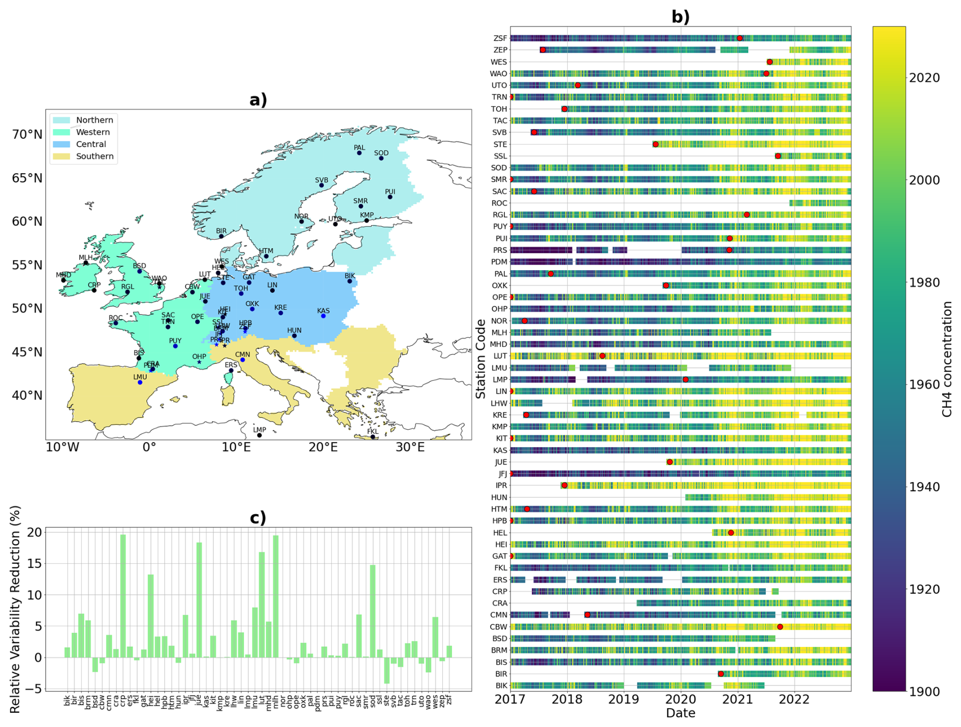
Figure 1Distribution of the CH4 observational network used in the inversion. Black markers indicate low-altitude stations (<1000 ), while blue markers represent high-altitude stations (>1000 ). Stations included in the sensitivity analysis are highlighted with star symbols. The EU27+3 countries are grouped into four sub-regions, as indicated by the color-coded legend. (b) Overview of daily mean CH4 mole fractions from each assimilated station, including the timing of ICOS labelling. Data points after the red marker are ICOS-labelled, indicating that measurements have been processed according to ICOS protocols from the indicated date onward. White gaps indicate periods with missing data. (c) Relative variability reduction (%) for each station, defined as , where σfull is the standard deviation over the full period (2017–2022), and σwindow is computed over 14:00–16:00 LT for low-altitude stations and 02:00–04:00 LT for high-altitude stations.
In cases where multiple intake heights were available, such as at the Cabauw station, where intakes were positioned at 27, 67, 127, and 207 m a.g.l., we chose to use data exclusively from the highest intake height. This approach was adopted to mitigate the difficulties that transport models encounter in accurately representing concentration gradients close to the ground, where such gradients tend to be steep and variable. By selecting the highest intake height, we ensured that the assimilated data more closely represent the characteristics of a well-mixed boundary layer, thereby improving the consistency of the modeled methane mole fractions (Vermeulen et al., 2011). Vertical gradients of CH4 near the surface are notoriously difficult to simulate accurately due to complex local meteorology, surface interactions, and diurnal variability (Peltola et al., 2015).
To further reduce these challenges, we use recommended quality-controlled observations during periods when vertical gradients are expected to be weaker, thereby minimizing potential transport model errors. For low-altitude sites (≤1000 ) over relatively flat terrain, we assimilate 3 h afternoon averages (14:00–16:00 LT), when the boundary layer is typically well mixed and vertical mixing is strong. For high-altitude or mountainous sites (>1000 ), we instead use 3 h nighttime averages (02:00–04:00 LT), which are more representative of free-tropospheric conditions and less affected by daytime valley winds that are difficult to resolve at coarse model resolution. By focusing on these time windows, we aim to reduce biases associated with shallow nocturnal boundary layers and unresolved slope and valley circulations, thereby improving the reliability of the assimilation.
This strategy is consistent with common practices in atmospheric inverse modeling, where daytime observations are generally preferred for lowland sites to avoid stable nocturnal conditions, while nighttime observations are often used in mountainous regions to limit the influence of unresolved diurnal circulations (Steiner et al., 2024; Monteiro et al., 2024). To further characterize temporal variability, we computed the standard deviation of CH4 mole fractions within these periods and quantified the relative reduction compared to the full daily variability (Fig. 1c). The mean standard deviation decreases from 39.4 ppb (range: 18.9–125.7 ppb) to 37.2 ppb (range: 18.8–103.8 ppb), corresponding to a mean reduction of 4.0 % (range: −4.2 % to 23.6 %). This indicates that the selected windows generally capture more stable atmospheric conditions, supporting their use in the inversion, despite some site-specific deviations.
2.4 Prior fluxes
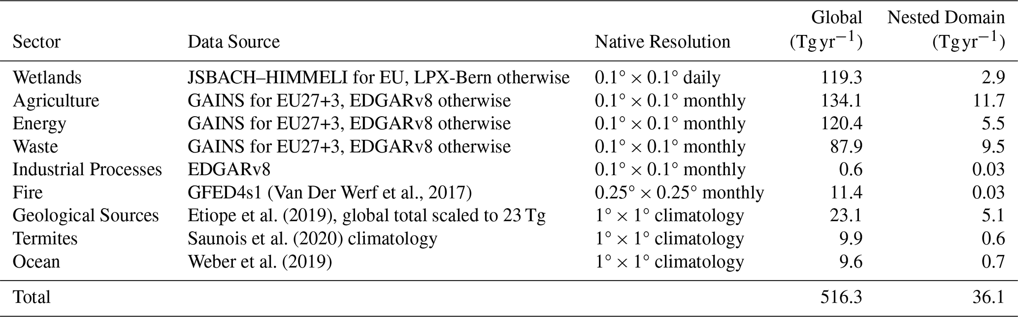
High-resolution monthly data are employed for key contributors (anthropogenic, biospheric and fire) to capture fine-scale spatial variability and to identify localized hotspots. For sources with sparse data availability and limited temporal variability (ocean, geological and termites), coarser climatological estimates are used. However, all datasets are regridded to match the inversion spatial resolution (0.2°×0.2° for the nested European domain and 2°×2° for the global background). The inversion is performed at monthly temporal resolution, optimizing fluxes independently for each month. Within the nested European domain, agriculture is the dominant source, contributing approximately 11.7 Tg yr−1 (estimates for 2020, 34 % of the annual regional total). Other major contributors include waste (9.5 Tg yr−1, 28 %), energy (5.5 Tg yr−1, 16 %), geological emissions (5.1 Tg yr−1, 15 %) and wetlands (2.9 Tg yr−1, 9 %), smaller contributions arise from ocean (0.7 Tg yr−1, 2 %), termites (0.6 Tg yr−1, 2 %), industrial processes (0.03 Tg yr−1, <1 %) and fires (0.03 Tg yr−1, <1 %), with all estimates in brackets corresponding to the year 2020. These individual source contributions are combined to derive the total prior CH4 emissions used in the total-flux inversion, while the sector-specific inversion optimizes each sectoral flux component separately within the expanded control vector. A comprehensive overview of the prior data is provided in Table 1, with the corresponding map of mean fluxes for 2017–2022 shown in Appendix A Fig. A1.
Table 1Overview of CH4 emission sources, their native resolutions, and average total emissions for the global and nested domains (Tg yr−1). The reported values correspond to 2020 prior emissions.
Monthly anthropogenic CH4 emissions are derived from the Emission Database for greenhouse gas and Atmospheric Research (EDGARv8.0) (Crippa et al., 2020) and Greenhouse Gas and Air Pollution Interactions and Synergies (GAINS) (Höglund-Isaksson et al., 2020) inventories, both providing high-resolution (0.1°×0.1°) global estimates of greenhouse gas emissions across multiple sectors. For EU27+3, we use emission estimates from the GAINS inventory, which incorporates country-specific activity data and mitigation assumptions, providing regionally consistent estimates that reflect national circumstances more closely than the globally uniform EDGARv8.0 inventory. On average, GAINS estimates are 3 Tg yr−1 (ranging from 1 to 4 Tg yr−1) lower than EDGARv8.0, amounting to approximately 10 % of the total anthropogenic CH4 emissions in the EU27+3 region during the study period. For categorising anthropogenic emission sources, we adopted the IPCC (2006) Common Reporting Format (CRF) to classify the emissions into four main sectors: Energy, Industrial Processes and Product Use, Agriculture, and Waste. This sectoral breakdown is consistent with UNFCCC NGHGI reporting guidelines and used by major inventories such as GAINS and EDGAR, allowing for direct comparison with national reports.
Biospheric emissions in our prior estimates are sourced from the JSBACH model, which simulates key ecosystem processes such as photosynthesis, respiration, carbon and water cycling, vegetation dynamics, and land ecosystem processes (Reick et al., 2021). Specifically, we use the version of JSBACH coupled with HIMMELI (Raivonen et al., 2017) (JSBACH-HIMMELI), which provides hourly methane emissions at high spatial resolution (0.1°×0.1°) over Europe. The modeled CH4 fluxes include contributions from peatlands, water-saturated and inundated soils, and net mineral soils, thereby representing the dominant diffuse terrestrial and freshwater-influenced methane sources. As the JSBACH-HIMMELI product used in this study provides data only for the European domain, we complement it with global biospheric emissions from the LPX-Bern DYPTOP v1.4 dataset (Lienert and Joos, 2018) to represent the global background.
Monthly prior fire emissions are obtained from the Global Fire Emissions Database version 4 (GFED4s) described in van der Werf et al. (2017) at a spatial resolution of 0.25°×0.25°, excluding methane emissions from biomass and agricultural waste burning, which were already included in GAINS and EDGAR. Oceanic CH4 emissions are represented by climatological estimates from Weber et al. (2019), while geological emissions are based on the dataset by Etiope et al. (2019), globally scaled to 23 Tg yr−1, following the Intergovernmental Panel on Climate Change (IPCC) AR6 Working Group I report (IPCC, 2023a; Tsuruta et al., 2023). Termite-related emissions are included according to the estimates provided by Saunois et al. (2020). The total flux constructed using the GAINS inventory for the EU27+3, combined with the other data sources listed in Table 1, is hereafter referred to as the “GAINS-based” prior.
2.5 Sensitivity Tests
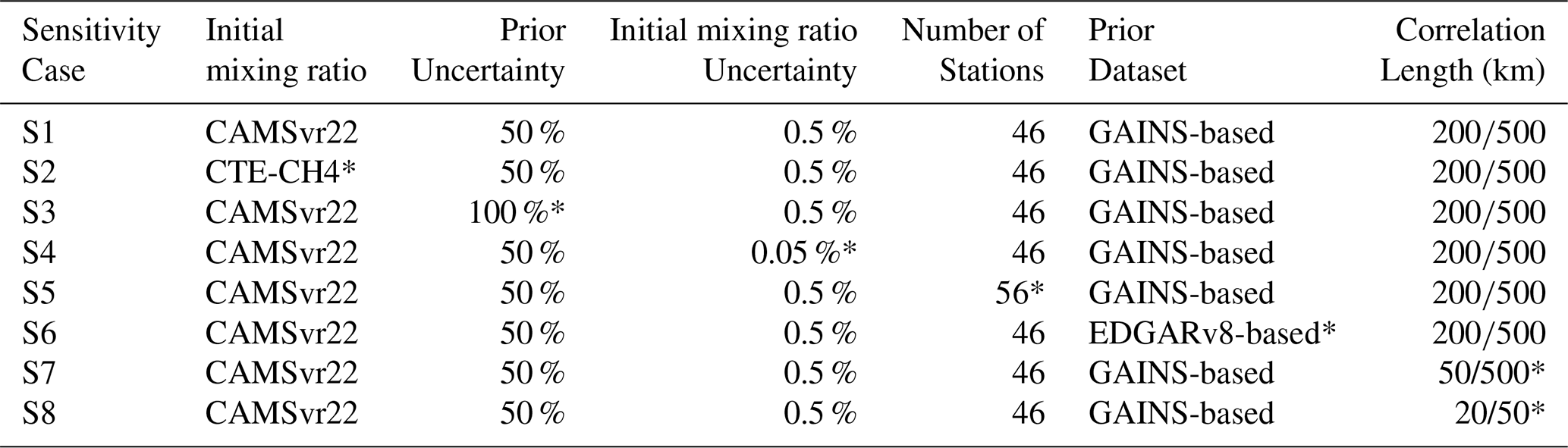
We conducted eight sensitivity experiments (S1–S8) for the total-flux inversion to evaluate how key elements of the inversion setup influence the posterior CH4 flux estimates and the associated error reduction. The base inversion (S1) serves as a reference for comparison. In S2, the initial CH4 mixing ratio fields from CAMSv22r2 (Bergamaschi et al., 2013) are replaced with those from CTE-CH4 (Tenkanen et al., 2025), both of which are outputs of global atmospheric inversion systems based on the TM5 transport model and available at daily resolution. In this study, we use these datasets for the 2017–2022 period. These fields are used to compute sensitivities to the mixing ratio at the endpoints of FLEXPART back-trajectories. This substitution allows us to assess the sensitivity of the inversion to the choice of initial mixing ratio and associated large-scale background representation. Although both products rely on TM5-based transport (Krol et al., 2005), they differ in their inversion configurations, including data assimilation methods, flux resolution, prior constraints, and assimilated observations. Inversions S3 and S4 address uncertainty assumptions. In S3, the prior flux uncertainty was increased from 50 % to 100 %, allowing more flexibility for the inversion to adjust emissions. In S4, the uncertainty assigned to initial mixing ratios was reduced from 0.5 % to 0.05 %, thereby increasing the influence of observed enhancements on the posterior flux adjustments. In S5, the observational network was expanded from 46 to 56 sites, including a denser station distribution along the Swiss Alps (see Fig. 1), to examine the sensitivity to observational coverage. In S6, the prior emissions were replaced from GAINS-based estimates to EDGARv8, which are approximately 10 % higher, allowing assessment of how differences in emission inventories affect the posterior flux estimates. Finally, S7 and S8 address spatial error correlations in the prior. The horizontal correlation length was reduced from 200 to 50 km (S7) and 20 km (S8), enabling finer spatial adjustments in the inversion. All inversions were performed using a 4D-Var ensemble approach, in which 30 Monte Carlo realizations were generated by perturbing both prior fluxes and observational data. Posterior uncertainties were estimated from the ensemble by approximating the posterior error covariance discussed in Sect. 2.1, Eq. (4). The error reduction was computed as , where σpost and σprior denote the posterior and prior uncertainties, respectively. Due to computational constraints, the sensitivity experiments were carried out for July 2021 only. This summer-month analysis is intended as a diagnostic evaluation of inversion-framework sensitivity and does not capture the full seasonal variability. A summary of the inversion configurations is provided in Table 2. The base inversion (S1) configuration is applied consistently throughout the study period, and the results presented in the total-flux analysis section are based on this setup unless otherwise stated. The sectoral inversion shares the same general configuration as the total-flux inversion but employs an extended control vector that explicitly decomposes emissions into individual source sectors, enabling simultaneous optimization of sector-specific fluxes within CIF-FLEXPART.
Table 2Inversion setups for the sensitivity analysis. Deviations from the base inversion (S1) are indicated with an asterisk (*).
3.1 Comparison of Simulated and Measured Methane Mole Fractions
Standard metrics such as mean bias, root-mean-square error (RMSE), and correlation play a crucial role in evaluating the performance of atmospheric inversion models by enabling direct comparison between simulated and observed CH4 mole fractions. In this section, these metrics are applied to assess the CIF-FLEXPART inversion simulated mole fractions against the assimilated in situ observations. Figure 2 displays time series of both prior and posterior mole fractions from the base inversion set-up, alongside observations from selected European in situ stations in 2021, which cover a range of geographical settings and emission regimes. The prior methane mixing ratios generally underestimate the observations, resulting in a mean negative bias at most sites, whereas the posterior estimates substantially reduce this bias.
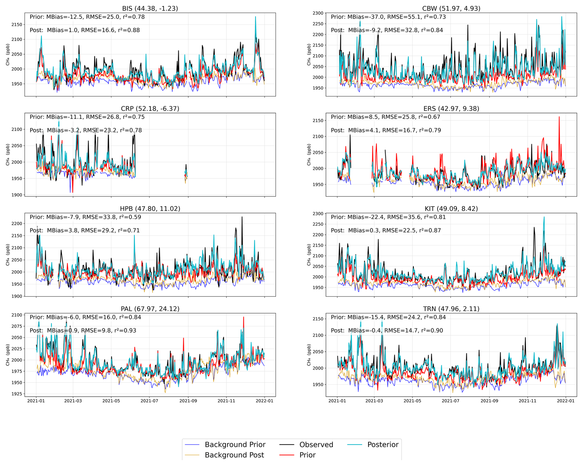
Figure 2Time series of observed and modeled CH4 mole fractions at selected stations, averaged at the assimilated hour for 2021: BIS (Biscarrosse, France), CBW (Cabauw, Netherlands), CRP (Carnsore Point, Ireland), ERS (Ersa, coastal Mediterranean site), HPB (Hohenpeissenberg, mountain station in Germany), KIT (Karlsruhe, Germany), PAL (Pallas, Finland), and TRN (Trainou, France), where the numbers in parentheses indicate the station's latitude and longitude. Shown are observations (black), prior simulations (orange), posterior simulations (green), and background contributions (cyan for prior, purple for posterior). Text boxes in each panel report mean bias (MBias) in ppb, root mean square error (RMSE) in ppb, and correlation coefficient (r2) for the prior and posterior relative to the observations.
These improvements are clearly visible in the time series shown in Fig. 2, illustrating the discrepancies between observed and prior-simulated mole fractions and their correction in the posterior. For instance, at stations BIS, CRP, HPB, KIT, and TRN, the prior exhibits a pronounced negative bias (−11.1 to −22.4 ppb) and systematically underestimates sharp observational peaks when regional fluxes are elevated. The prior initial concentration contribution is overly smoothed and lacks the sharp variability of the observed and simulated mole fractions, though it still shows meaningful variations. In contrast, the posterior reduces these biases (mean bias −3.2–3.8 ppb) and improves the representation of both the initial condition and regional flux contributions, providing a more realistic depiction of the regional signal. This adjustment is further reflected in the corresponding flux contributions in Appendix A Fig. A2, where regional fluxes are increased in the posterior to better match the observations. At CBW, where local influences dominate, the prior fails to reproduce the full variability (see Fig. 2, CBW); the posterior reduces the overall bias, although some high-frequency discrepancies persist. The regional flux contributions show substantial adjustments in the posterior, consistent with the improved match to observations. At PAL, prior mole fractions generally match observations, but pronounced mismatches occur during the first months of 2021. These are largely corrected by adjustments to the initial concentration contribution, while the global flux contribution remains relatively more influential and unchanged in the posterior (see Appendix A Fig. A2). At ERS, unlike most other stations, the prior exhibits a mean positive bias of 8.5 ppb, which is reduced to 4.1 ppb in the posterior. The background contribution is adjusted upward, reinforcing the positive bias, while the regional flux contribution is lowered in the posterior. Together, these adjustments improve the overall agreement between simulated and observed mole fractions, illustrating the inversion's ability to correct both the initial condition and the regional flux components. Overall, these results demonstrate that the inversion effectively corrects biases in both the initial conditions and the regional fluxes, improving the representation of CH4 dynamics across stations.
These station-level mole fractions are further illustrated in Fig. 3, which evaluates model–observation agreement across all stations and years (2017–2022). The coefficient of determination (R2) increased from 0.54 to 0.76, RMSE decreased from 33.4 to 24.4 ppb, and mean bias was reduced from −12.2 to −2.1 ppb. The posterior regression slope (0.75) is closer to unity than the prior (0.57), and Pearson correlation increased from 0.78 to 0.87 (p<0.001), reflecting enhanced responsiveness to observed changes. Modelled vs. observation performance metrics for all assimilated stations are summarized in Appendix A Table A3. Our posterior statistical results closely align with the findings of Steiner et al. (2024), Bergamaschi et al. (2022). By assimilating data from 28 stations, Steiner et al. (2024) reported a Pearson correlation of approximately 0.7 for 25 of the stations. Figure 3 also reveals that the prior simulation systematically underestimates high CH4 mole fractions, with many data points falling below the regression line. This underestimation is particularly pronounced at stations such as LUT, LMU, STE, and CBW, all of which exhibit strong negative biases (below −35 ppb). Although the posterior simulation substantially reduces this underestimation, with biases improving to around −10 ppb, some discrepancies persist at the highest mole fractions, likely reflecting unresolved local emissions or sub-grid variability. These results highlight the importance of targeted improvements in emission inventories and model resolution for stations with persistent negative bias.
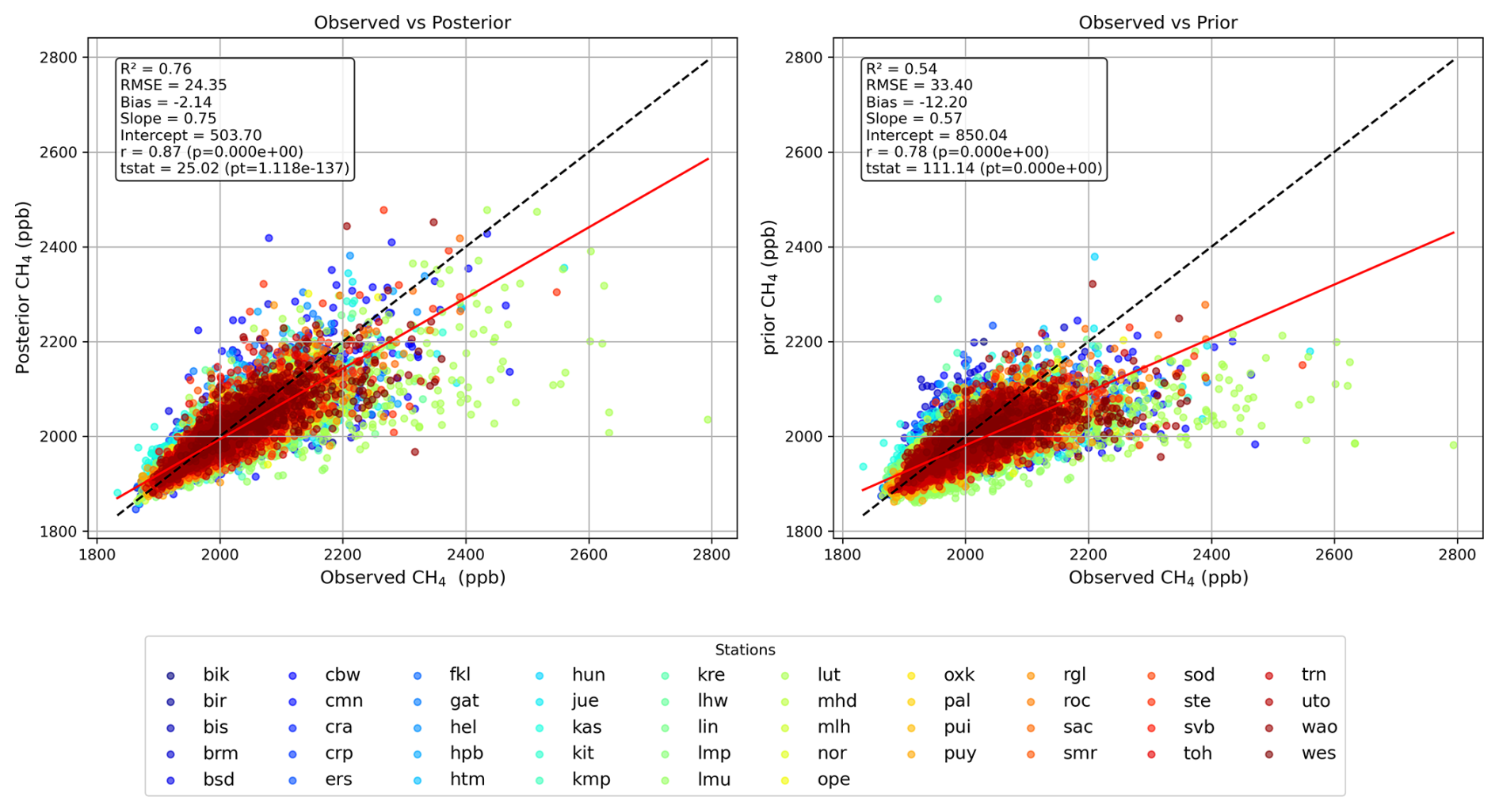
Figure 3Modeled vs. observed CH4 mole fractions for all assimilated in situ observations. Left panels: posterior vs. observations; right panels: prior vs. observations. Statistical metrics are shown in each panel. Black dashed line: one-to-one; red line: best-fit regression.
To further assess the level of agreement across subregions, we compare posterior and prior simulations for different categories. This includes geographical regions (Central, Northern, Western, Southern) consistent with Petrescu et al. (2021), as well as elevation (mountain vs. non-mountain) and station type (coastal vs. non-coastal). Figure 4 presents the distributions of residuals using violin plots, with the 25th–75th interquartile range indicated by a vertical line. Posterior residuals exhibit systematically narrower spreads and improved alignment with observations. Across regions, RMSE and interquartile range (IQ75) decrease by 26 %–37 %, with median residuals moving closer to zero, except in the Southern region. Mountain stations show a smaller spread reduction (IQ75: 21.5 vs. 27.6, RMSE reduction 26 %), reflecting higher variability likely due to complex transport, whereas non-mountain, coastal, and non-coastal stations show 28 %–32 % RMSE reductions. Overall, these analyses demonstrate that the inversion effectively reduces uncertainty and bias across all categories, enhancing model fidelity and observational agreement (see Table 3).
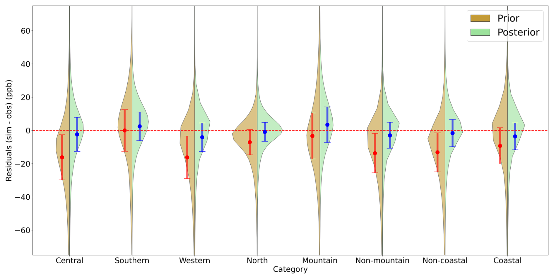
Figure 4Residuals between observed (obs) and modelled (sim) CH4 concentrations for assimilated in situ stations, grouped by subregional category (see Appendix A TableA2) The horizontal dashed line indicates zero residual, and the vertical bar shows the 25th–75th interquartile range. Negative values indicate that simulated concentrations are lower than observed.
Table 3Prior and posterior performance metrics of CH4 mole fraction simulations from the total flux inversion setup grouped by sub-regional category (see in Appendix A Table A2). Reported statistics include regional mean bias, the interquartile ranges: the 25th–75th (IQ75), and the 5th–95th range (IQ95), root mean square error (RMSE), relative RMSE reduction (ΔRMSE), number of observation stations, and the total number of data points (N-data) used in the evaluation.

3.2 Posterior Flux
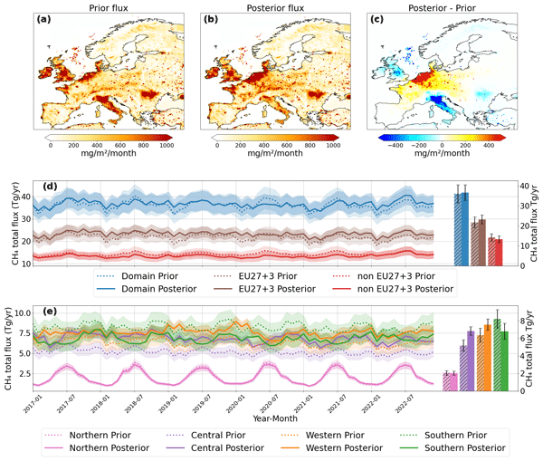
In Fig. 5, we presented the six-year mean methane fluxes (2017–2022) over the study domain. Figure 5a–c display prior estimates, posterior estimates, and their differences, while Fig. 5d–e present monthly time series and inland average estimates for subregions. The spatial maps highlight regions of substantial flux adjustments, and the time series illustrate temporal variability and regional contrasts between prior and posterior estimates. The inversion reveals pronounced regional corrections, with posterior emissions being systematically higher over BENELUX, France, and Germany, pointing to underestimation in the prior, whereas reductions occur over the UK, Italy, and Romania, indicating prior overestimation. These patterns align well with earlier inversion studies (Bergamaschi et al., 2022; Steiner et al., 2024). In regions with sparse observational data, such as the Iberian Peninsula and eastern Europe, the prior fluxes change only slightly.
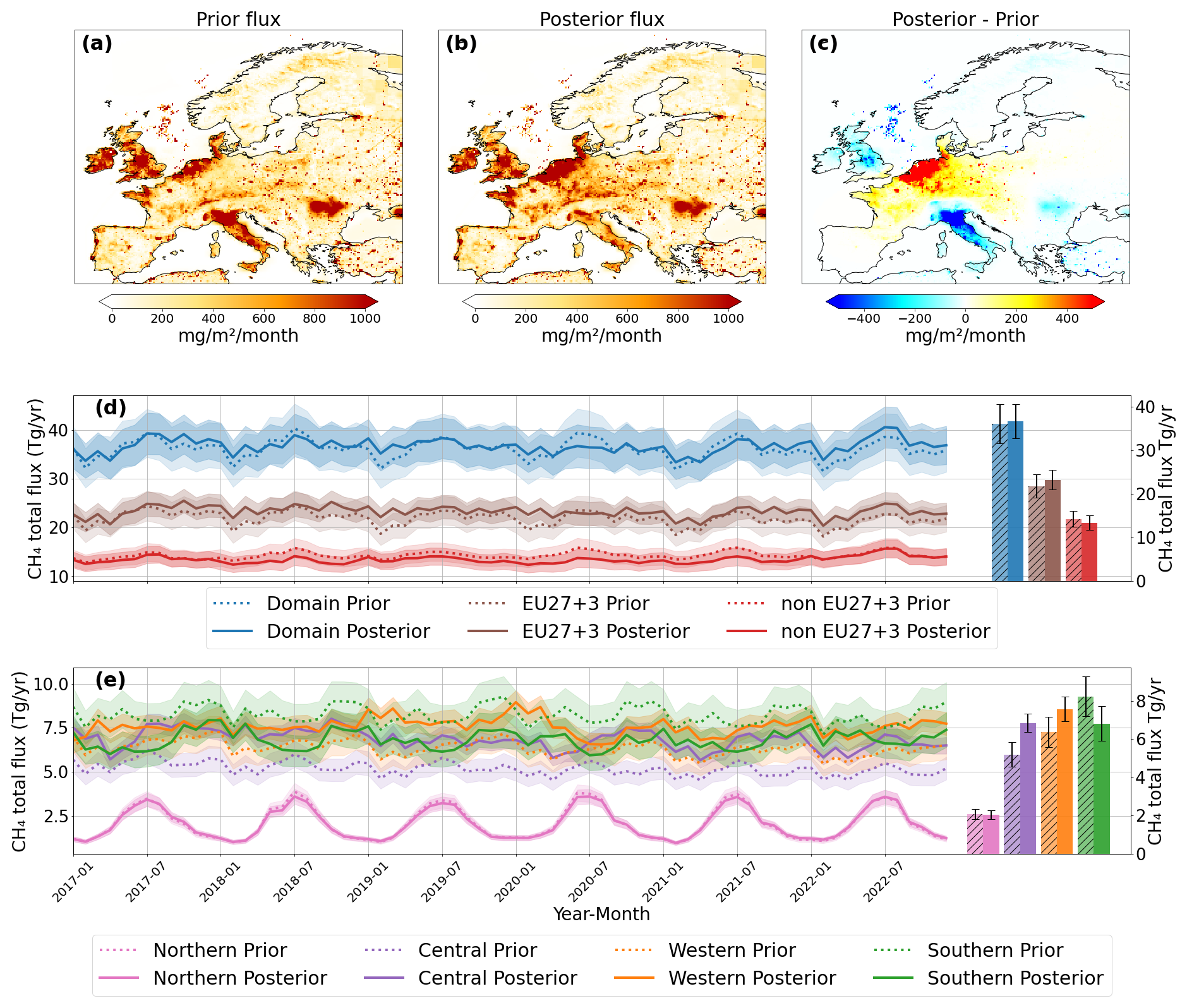
Figure 5Top row: Mean methane (CH4) fluxes over the EU27+3 domain for the study period (a) prior fluxes, (b) posterior fluxes after inversion, and (c) flux increments (posterior – prior). Middle rows: Monthly CH4 flux time series averaged over the entire domain, within EU27+3, and outside EU27+3. Bottom row: Monthly CH4 flux time series for selected EU27+3 subregions (Northern, Central, Southern, and Western), showing prior (dashed lines) and posterior (solid lines) estimates. Bars on the right summarize mean annual prior and posterior fluxes estimates. Shaded areas denote the corresponding prior and posterior uncertainties in the time series, while error bars on the bars represent the associated annual uncertainties.
Despite these pronounced regional adjustments, the mean emission exhibits only a modest net change at the domain scale, with average total methane emissions shifted 36.1±4.5 Tg yr−1 in the prior to 36.7±4.0 Tg yr−1 in the posterior, a rise of 1.7 % (see Fig. 5d), reflecting strong subregional contrasts. Notable posterior CH4 flux increases are observed in Central Europe (+32 %) and Western Europe (+19 %), in contrast, Southern Europe shows a decrease of 17 % (see Fig. 5e). The monthly time series reveals a clear seasonality in northern regions, with a peak in summer months. The southern region exhibits a slight opposing seasonality, while other regions show no clear seasonal cycle. Additionally, it displays that posterior emissions from Central and Western Europe are consistently higher than the prior throughout the study period, while in the southern region, the posterior emissions are generally lower than the prior. At the domain and EU27+3 scales, however, there is no clear or persistent difference between posterior and prior emissions, and no significant trend is evident over the 2017–2022 period at either the domain or subregional scale. Over the EU27+3, the average posterior flux for 2017–2022 is 23.3±2.3 Tg yr−1, representing a 6.6 % increase relative to the prior (21.7±2.7 Tg yr−1). Our results falls within the 22–26 Tg yr−1 range reported by Petrescu et al. (2021), Petrescu et al. (2023) for 2006–2017 based on three inversion setups. Although our estimate is at the lower end of this range, it provides a meaningful comparison given the difference in time periods, as EU27+UK emissions show no strong trend over the interval considered.
While spatial patterns in total methane flux adjustments indicate where the inversion has modified prior estimates, analysing these changes by sector reveals the dominant sources driving regional flux adjustments and highlights systematic biases in prior inventories. Figure 6 presents the spatial distribution of sector-specific methane flux increments (posterior – prior) over Europe for 2017–2022. Panels (a)–(d) correspond to anthropogenic sectors: agriculture (AGR), energy (ENG), waste (WST), and industry (IND); whereas panels (e)–(g) depict natural sources, including wetlands (WET), geological seepage (GEO), and biomass burning (FIR). Posterior agricultural emissions increase markedly across the BENELUX region, suggesting systematic underestimation in the prior inventory. Adjustments in other anthropogenic sectors are generally more spatially localized. Energy-related emissions decrease over the North Sea, but localized increases are observed in Belgium, Luxembourg, Ukraine, and western Russia. Waste emissions show localized hotspots in BENELUX, France, and Poland, while decreasing in Italy and the UK. Industrial emissions rise predominantly over BENELUX and Germany. CH4 emissions from wetland are reduced, particularly in northern Europe and the UK, largely reflecting a reduction in summer fluxes. Reductions in the GEO sector over Italy and Romania are consistent with previously reported overestimations arising from the global scaling of geological emission factors. Steiner et al. (2024) likewise identified strong posterior reductions over Italy and Romania, which they attributed to inflated geological emissions in these regions. Although prior geological emissions were harmonized to 23 Tg yr−1 at the global scale, the inversion results highlight the need for regionally differentiated emission estimates. Footprint sensitivities from FLEXPART (Appendix, Figs. A3–A4) reveal a heterogeneous observational constraint, with moderate sensitivities in Italy and Romania. Nevertheless, substantial flux corrections are inferred due to the combination of moderate footprint sensitivities and relatively large prior geological emissions, yielding sufficient emission sensitivity to drive posterior adjustments.
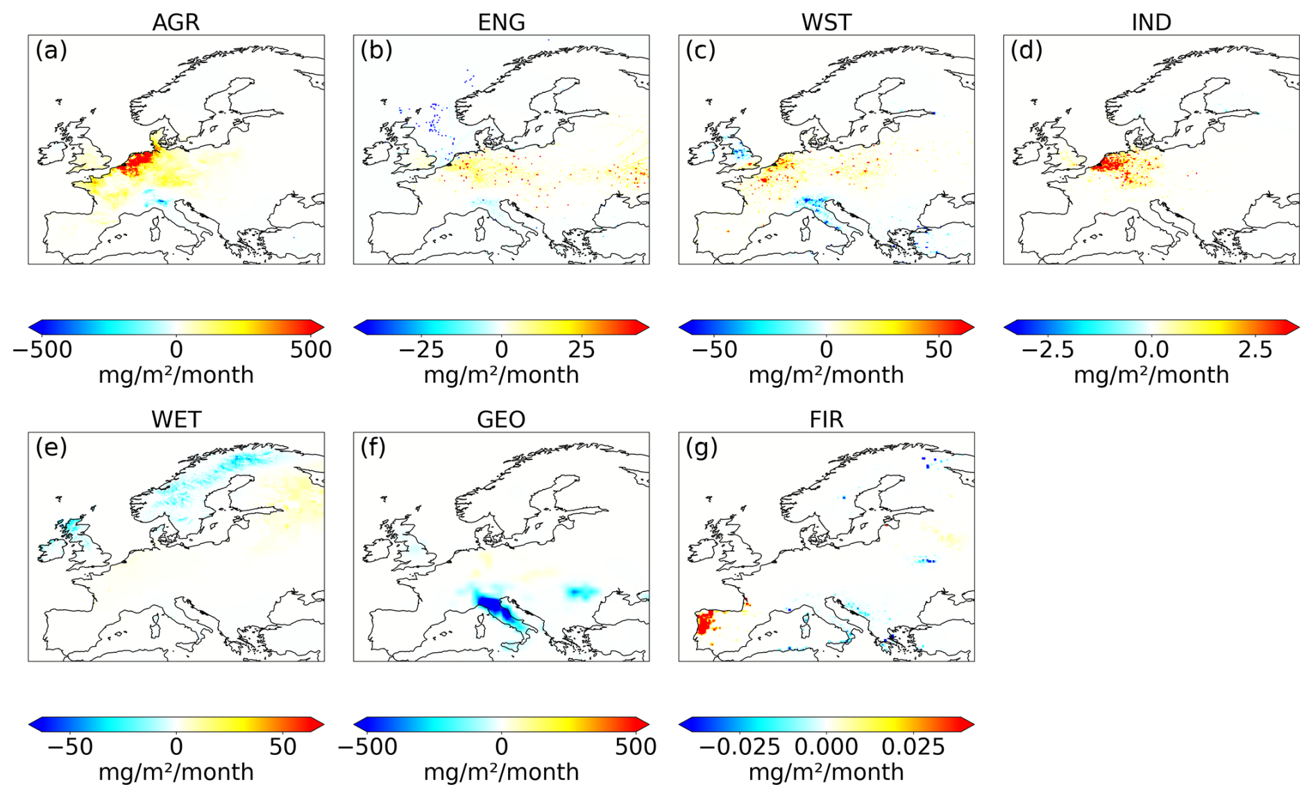
Figure 6Spatial distribution of sector-specific methane flux increments (posterior – prior) over Europe averaged in the years (2017–2022). Panels show adjustments for agriculture (AGR), energy (ENG), waste (WST), industry (IND), wetlands (WET), geological sources (GEO) and fires (FIR). Agricultural emissions exhibit the largest posterior increase, particularly across central and western Europe, whereas wetlands show strong reductions in northern Europe. Geological emissions decrease mainly in southern Europe and Romania. Note that the colour scale is different.
Figure 7 summarizes the prior and posterior fluxes by European subregion. Agricultural emissions show the largest positive adjustments. In central EU27+3, emissions increase from a prior estimate of 2.4 to a posterior estimate of 3.2 Tg yr−1 (+33 %), and in western EU27+3 they rise from 3.5 (prior) to 4.5 Tg yr−1 (posterior), which is a 29 % rise. The strongest relative increase occurs in the BENELUX region, where mean agricultural emissions nearly double from 0.7 to 1.3 Tg yr−1 (+86 %). At the domain scale, posterior agricultural CH4 emissions amount to 13.6 Tg yr−1, representing a 16 % increase compared with the prior. EU27+3 posterior emissions are estimated at 10.8 Tg yr−1, corresponding to a 21 % increase relative to the GAINS prior (Fig. 7a). Agricultural emissions account for 46 % of the total EU27+3 CH4 budget in our estimate, representing the largest sectoral share. This aligns with consolidated assessments and UNFCCC NGHGI reports, which attribute 52.4 % (±8.7 %) of EU27+UK CH4 emissions in 2019 to agriculture (Petrescu et al., 2021, 2023). The dominant role of agriculture in total anthropogenic CH4 emissions also holds globally (IPCC, 2019). Emissions from energy-related sectors show modest increases in central Europe, rising from 0.8 to 0.9 Tg yr−1 (+12 %), and in western Europe, the prior estimate of 0.3 Tg yr−1 remains effectively unchanged in our posterior at this precision. In contrast, emissions decrease over oceanic regions from 1.4 to 1.2 Tg yr−1 (−14 %), largely reflecting reduced fossil fuel contributions (Fig. 7b). Waste-sector emissions show relatively minor adjustments at the regional and subregional scales, reflecting compensating regional contrasts. Posterior corrections are nevertheless evident in specific hotspot regions (Fig. 7c), with increases in BENELUX, France, and Poland, and decreases in the UK and Italy, highlighting substantial country-level heterogeneity. Wetland emissions in northern Europe were obtained to be 1.1 Tg yr−1 with no discernible change at this precision. However, notable summer reductions occur in northern Europe, as well as in the UK, Ireland, Italy, and coastal areas, indicating minor overestimations in these regions. In contrast, increases are observed in Eastern Europe and BENELUX (see Fig. 7d). CH4 emissions from geological seepage decline sharply in southern Europe, from 2.8 Tg yr−1 in the prior estimate to 1.5 Tg yr−1 in the posterior, representing a 46 % reduction, primarily driven by substantial prior overestimated emissions from Italy and Romania (Steiner et al., 2024) (see Fig. 7e). Details of regional and sectoral posterior fluxes estimates are provided in Appendix A Table A4. Total CH4 emissions increase at the EU27+3 level, mainly in western and central Europe, while decreases occur in southern and oceanic regions (Fig. 7f). Overall, these posterior flux adjustments highlight that anthropogenic activity, especially emissions from agriculture and waste, drives most of the net increase in CH4 emissions, while geological emissions decrease. These heterogeneous corrections underscore the importance of refining prior emission patterns at both sectoral and regional scales to develop robust methane budgets for Europe.
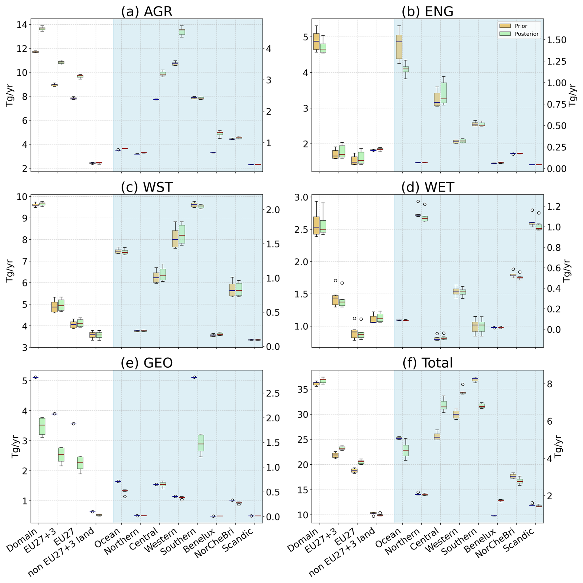
Figure 7Mean estimates of prior and posterior CH4 fluxes averaged over Europe and its subregions for the years 2017–2022. The panels display boxplots for total CH4 emissions (Total), agriculture (AGR), energy (ENG), waste (WST), wetlands (WET), and geological sources (GEO). The Total emissions are derived from the total-flux inversion, whereas the sectoral emissions are obtained from the sector-specific inversion. Boxplots within the lightblue-shaded area of each subpanel (Ocean–Scandic) correspond to smaller regions and are plotted against the right-hand y axis. The boxplot ranges represent temporal variability over the study period.
3.3 Temporal Variation of CH4 Flux
Figure 8 illustrates the seasonal patterns of CH4 emissions from the Agriculture, Energy, Waste, and Wetlands sectors, spatially aggregated across the EU27+3 subregions. Among these, the Wetlands sector in Northern Europe exhibits the most pronounced seasonality, with emissions peaking during the summer months, particularly in July. This pattern is primarily driven by warmer temperatures and consistently sufficient soil moisture, which together enhance microbial activity and methane production in wetland ecosystems (Bechtold et al., 2025; Aalto et al., 2025). The accelerated decomposition of organic matter under these conditions further contributes to elevated emissions during this period (Voigt et al., 2023). The red hatched shading in the figure indicates a posterior reduction in summer wetland emissions, suggesting a downward correction of potentially higher prior estimates in summer. The Waste sector shows notable seasonal patterns, particularly in Central EU27+3 countries, where emissions increase significantly during summer. This is likely due to intensified microbial decomposition of organic waste in warmer temperatures, leading to greater methane generation in landfills and wastewater treatment facilities. In contrast, the Southern EU27+3 countries display a distinct summer minimum in waste emissions, highlighting regional differences that may be influenced by climate or waste management practices. Emissions from the Energy sector exhibit an opposite seasonal trend, with a clear peak during the winter and a minimum in summer. This pattern is largely attributed to increased heating demand in colder months, resulting in higher fossil fuel combustion and methane emissions. Additionally, winter energy use often involves greater reliance on natural gas, which can lead to methane leakage from pipelines and storage systems, further contributing to wintertime emission peaks. Recent studies support this seasonal behaviour. For example, Hu et al. (2025) found that oil and gas methane emissions can be substantially higher in winter, with estimates indicating increases of up to 40 % compared to summer. Similarly, Varon et al. (2025) reported pronounced seasonal variability in methane emissions from oil and gas production regions based on satellite inversions. These findings provide independent observational evidence supporting the wintertime enhancement of energy-sector methane emissions inferred in this study. These contrasting seasonal dynamics between sectors may counterbalance one another, contributing to the lack of a clear overall seasonal pattern in total CH4 emissions at the regional scale. The Agriculture sector, by comparison, does not exhibit a distinct seasonal pattern across any of the regions. However, hatched blue shading in the figure indicates posterior increases in agricultural emissions over Central and Western EU27+3 countries, suggesting model adjustments based on observational constraints. These regional and sector-specific variations underscore the complexity of CH4 emission dynamics and highlight the importance of disaggregated analyses to improve understanding and model representation of seasonal fluxes.
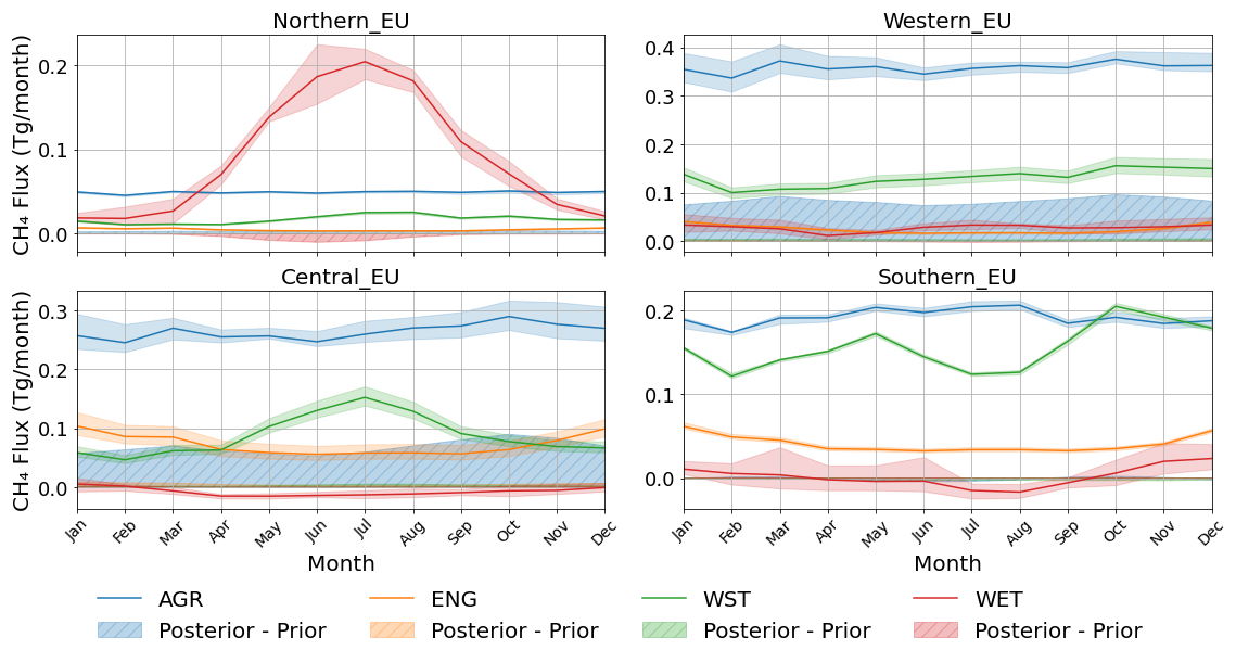
Figure 8Seasonal patterns of CH4 emission from major sectors, aggregated over the subregions for 2017–2022: (a) northern, (b) western, (c) central, and (d) southern Europe. The solid line represents the multi-year monthly mean, while the shaded area indicates the interannual variability (standard deviation). The hatched area shows the difference from the prior.
3.4 EU27+3 CH4 Emission Estimates and Comparison with UNFCCC Reports
We calculated country-level anthropogenic CH4 emission estimates for the EU27+3 and compared them with EDGARv8, GAINS, and UNFCCC NGHGI (2023) reports. Our posterior estimates averaged 17.6 Tg yr−1 for 2017–2021 (range: 17.0–18.2), with a mean annual decline of 0.3 Tg yr−1. These posterior estimates are 11 % higher than GAINS, 4 % higher than EDGARv8, and 3 % higher than UNFCCC, indicating good overall consistency at the EU27+3 scale. They are also in close agreement with previous inversion studies; for example, Steiner et al. (2024) reported 17.4 Tg yr−1 for EU27+UK in 2018, compared to our estimate of 17.6 Tg yr−1 for the same region and year. The top three emitting countries (France, Germany, and the UK) accounted for 39 % of EU27+3 emissions, similar to inventories but with differing country rankings. The UK stood second in the UNFCCC report. However, larger discrepancies appear at the national level (see Fig. 9 and Appendix A Table A5). Compared with UNFCCC, posterior emissions are higher for BENELUX (+54 %), Germany (+37 %), and France (+10 %), but lower for Romania (−25 %), Poland (−16 %), and Italy (−11 %). Notable differences also occur in the Nordics, with decreases in Norway (−39 %), Finland (−16 %), and Denmark (−13 %), but an increase in Sweden (+10 %). These national-scale differences are consistent with the findings of East et al. (2025), who compared inversion-derived methane emissions with UNFCCC inventories and similarly reported both positive and negative deviations at the country level across Europe. Their results underline the value of atmospheric inversion approaches for identifying potential biases and uncertainties in national methane emission reporting. Relative to EDGARv8, posterior estimates are higher for Portugal (+40 %), Italy (+18 %), and Germany (+10 %), but substantially lower in the UK (−18 %), Poland (−7 %), Romania (−18 %), and especially the Nordics. Adjustments relative to GAINS are upward for Germany (+29 %), France (+16 %), and BENELUX (+40 %), but downward for Switzerland (−13 %) and Italy (−7 %).
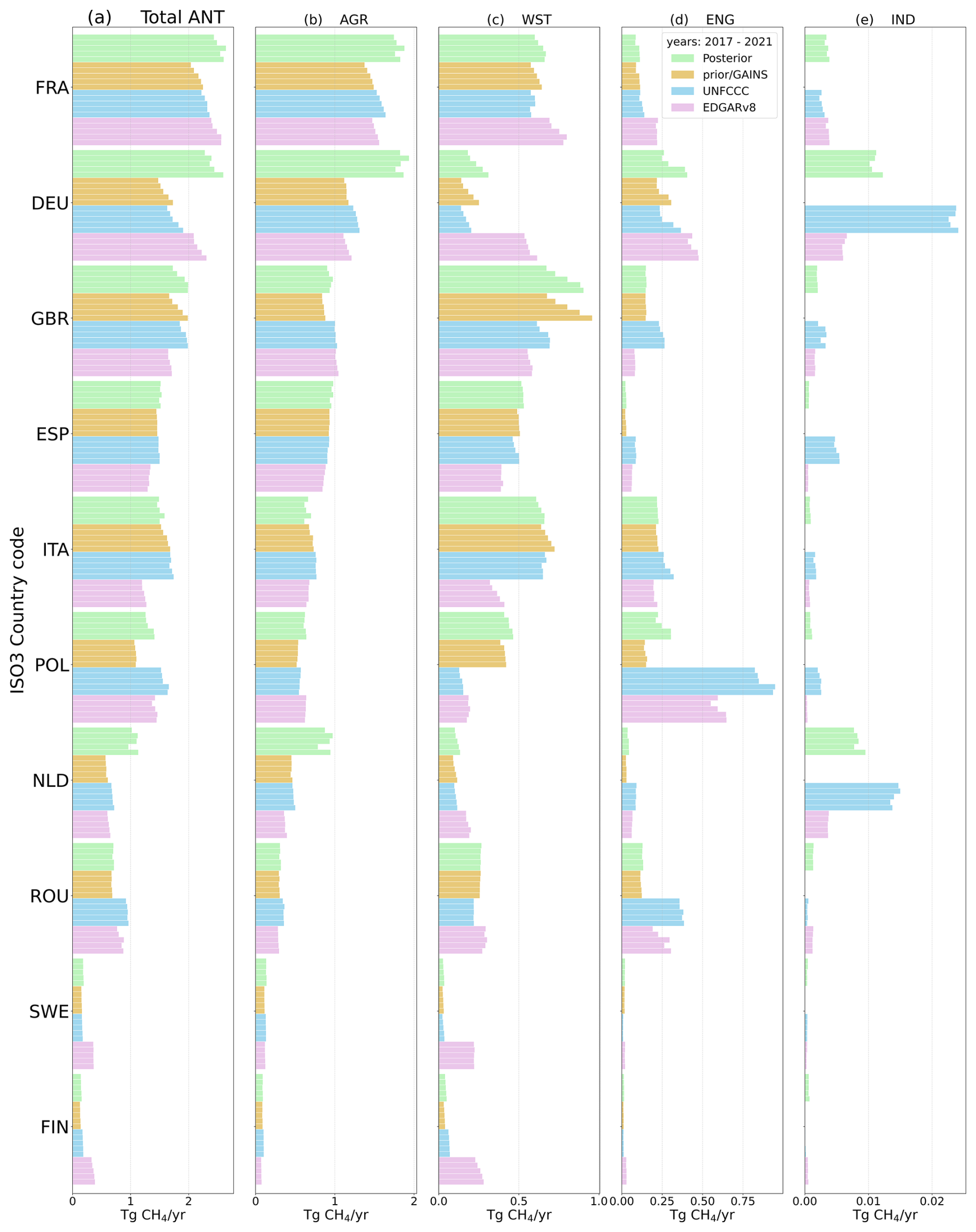
Figure 9Annual mean anthropogenic CH4 emissions (2017–2021) for selected EU27+3 countries, shown as bar plots for the posterior estimates, GAINS, UNFCCC, and EDGARv8. Subpanels display CH4 emissions from major anthropogenic sectors: (a) total anthropogenic emissions excluding land-use and land-cover change, (b) agriculture, (c) waste, and (d) energy. For each country and sector, bars of the same color represent a given dataset and are stacked by year, from bottom (2017) to top (2021).
In addition to country-level discrepancies in total anthropogenic estimates, systematic patterns emerge across sectors, as displayed in Fig. 9. In agriculture, inventories generally underestimate emissions in large agricultural countries such as France, Germany, and the Netherlands, whereas our posterior consistently suggests higher values. This implies that bottom-up activity data and emission factors may not fully capture agricultural methane sources. In the waste sector, EDGARv8 tends to overestimate emissions in countries like Germany and France but underestimates them in others, including the UK, Italy, and Poland. Our posterior estimates often fall closer to GAINS and UNFCCC values. For the energy sector, inconsistencies are more pronounced. In the UK, EDGARv8 clearly overestimates emissions, whereas in Poland and Romania, both EDGARv8 and UNFCCC report higher values than our posterior. These differences are likely driven by variations in fossil fuel activity data and the emission factors employed by different reporting frameworks. Overall, the EU27+3 total appears relatively robust across inventories, yet sectoral and country-level comparisons reveal significant discrepancies. Our inversion estimates provide an essential independent constraint in this context, helping to reconcile inconsistencies in bottom-up reporting systems and strengthening confidence in national and sectoral methane emission estimates.
3.5 Sensitivity Experiments and Their Impact on Optimised Flux Estimates
To assess the sensitivity of the inversion framework, we conducted eight inversions (S1–S8) by varying key parameters, including background mole fractions, prior flux and background mole fraction error assumptions, observational coverage, choice of prior inventories, and correlation assumptions detailed in Sect. 2.5. Figure 10 presents the resulting posterior flux increments and error reductions for July 2021; this one-month analysis is intended to compare sensitivity across different setups rather than to provide a detailed uncertainty estimate. Inversion setups from S1 to S5 exhibit broadly consistent spatial patterns and magnitudes of posterior flux increments, though the degree of error reduction varies among cases. The base inversion setup (S1) achieves substantial reductions of 14 % for Europe and 21 % for EU27+3, with particularly strong constraints in Central Europe (38 %) and Western Europe (30 %) (see Table 4). S2 is nearly indistinguishable from S1 at both regional and subregional scales, showing only slightly weaker reductions in northern Europe, suggesting that posterior adjustments are relatively insensitive to the choice of background concentration. S3 and S4 yield somewhat weaker mean error reductions of about 16 % for EU27+3, indicating moderate sensitivity of posterior adjustments to prior uncertainty scaling and background error assumptions. Larger assumed background errors allow observations to exert a stronger influence, whereas smaller errors suppress corrections and increase reliance on the prior. Although these effects are modest in magnitude (−2 to +2 ppb), they highlight the critical role of background error settings in modulating inversion flexibility and posterior responsiveness. The influence of background error settings on concentration fields is illustrated in Fig. 11.
Table 4Prior, Posterior, and Mean Error Reduction (%) for different regions and sensitivity inversion setups (S1–S8) as described in Sect. 2.5.
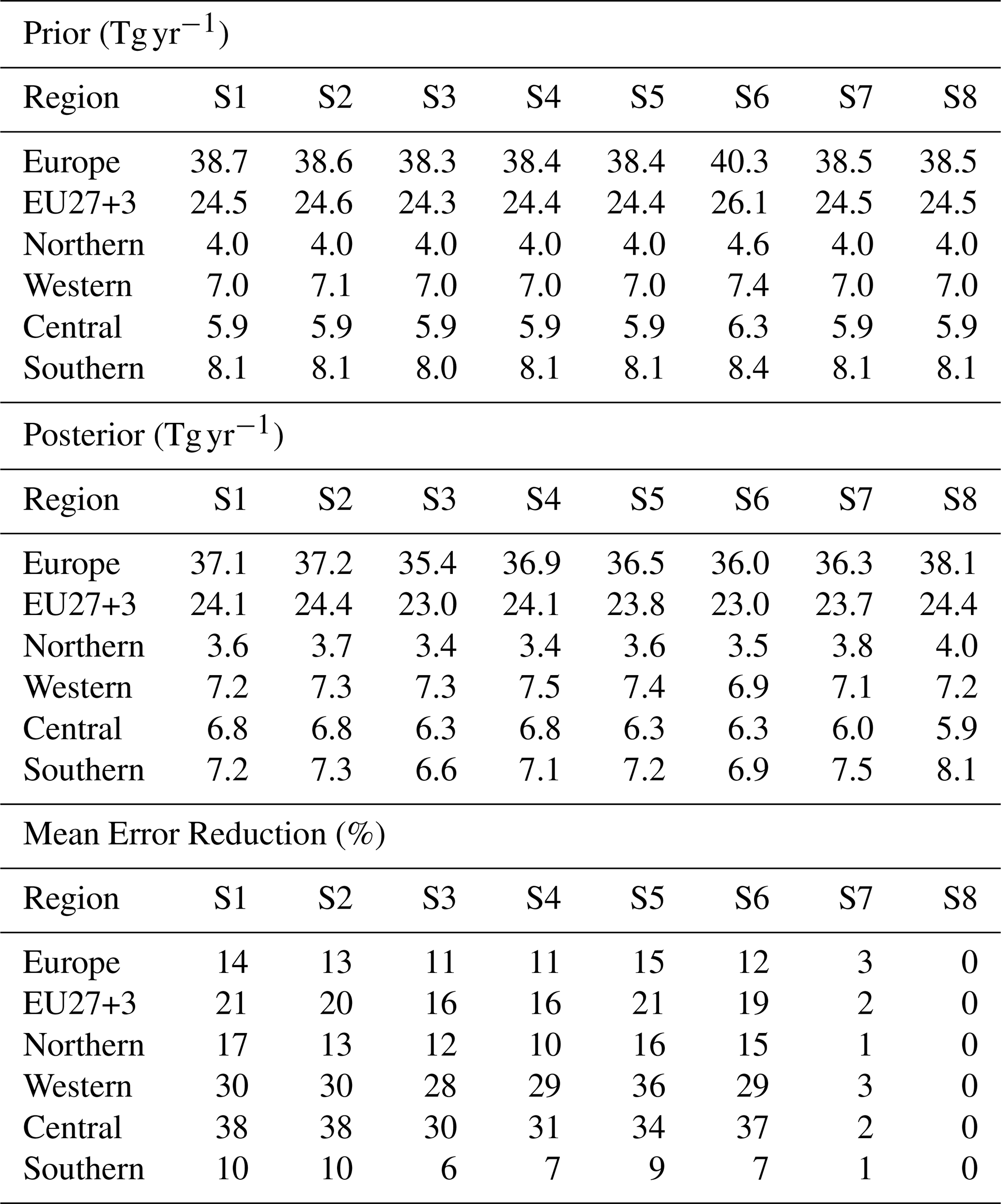
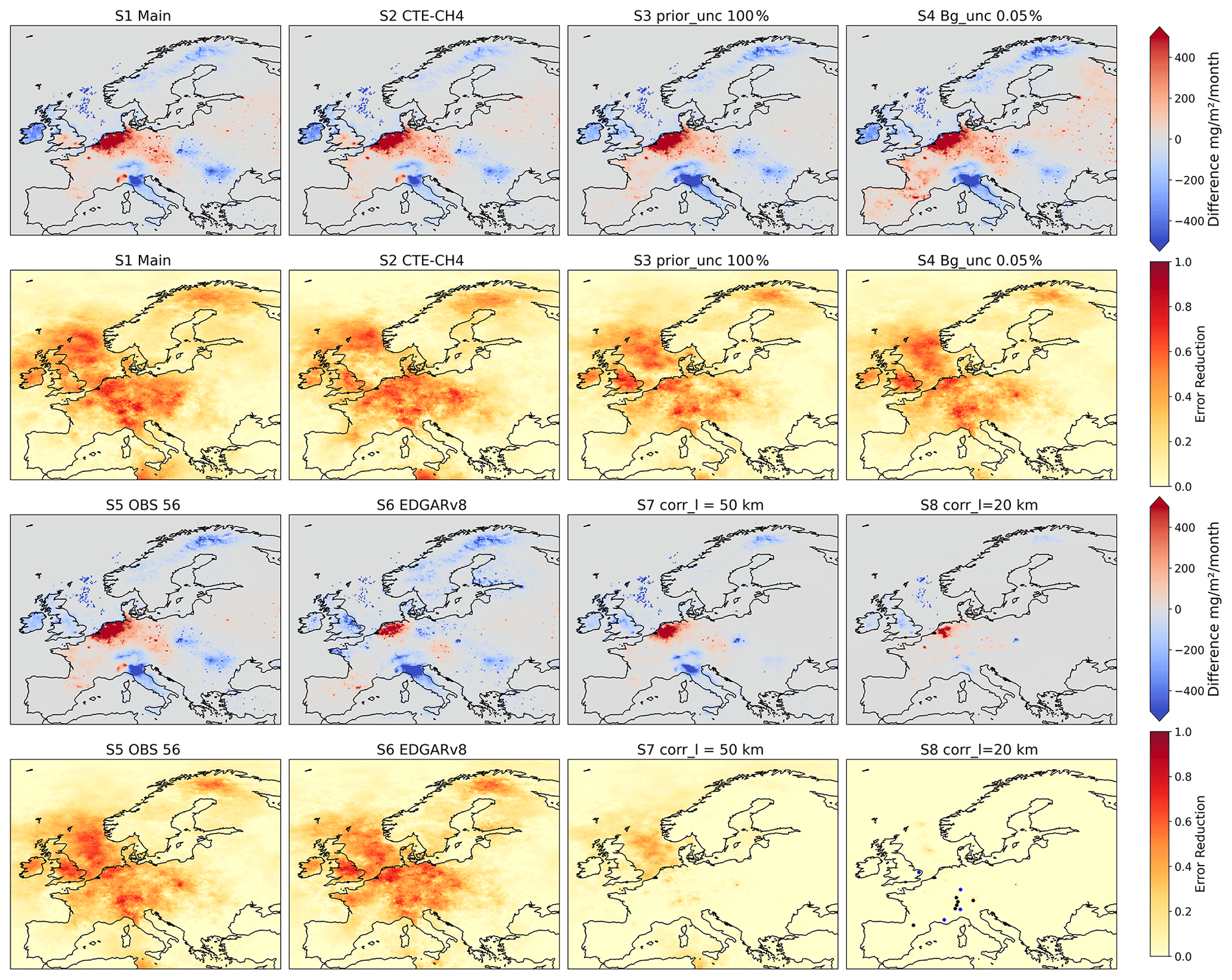
Figure 10Flux increments (posterior – prior) and error reduction for July 2021 across eight sensitivity inversion setups (S1–S8). Each panel illustrates the spatial distribution of flux adjustments relative to the prior, highlighting the influence of varying prior emissions, background treatment, observational network density, and error correlation assumptions. The last subpanel displays the stations added for inversion setup S5. Mountain stations are shown as black dots, while low-altitude stations are shown as blue dots.
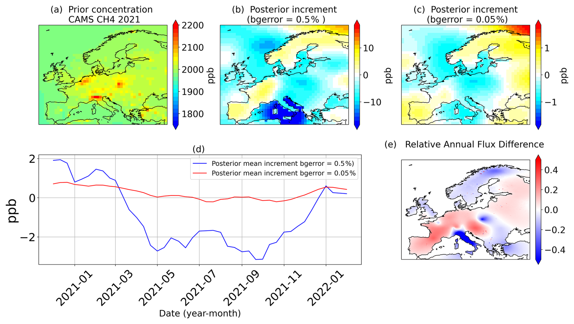
Figure 11Impact of background error assumptions on optimized methane mole fractions and fluxes for 2021. Top row: (a) Prior mole fractions from CAMS and posterior increments with background error assumptions of (b) 0.5 % and (c) 0.05 %. Bottom row: (d) Time series of posterior mean increments under both settings and (e) relative annual flux difference between inversions with background errors of 0.5 % and 0.05 %. To quantify the impact of background-error assumptions, the relative difference was defined as , where F0.5 % and F0.05 % denote the flux computed using a background-error assumption of (0.5 %) and (0.05 %) respectively.
Network densification in S5 enhances error reduction across most regions, particularly in Western Europe, where reductions exceed 35 %. This improvement reflects the added influence of stations such as TAC in the UK and PDM and OHP in France, which help better constrain emissions over the UK and southern France. The additional mountain station in the Alps, however, does not show a clear enhancement in posterior uncertainty reduction, suggesting that its effectiveness may depend on representativeness or transport model resolution. Although the spatial pattern of posterior flux increments remains consistent with earlier inversion setups, the expanded network clearly strengthens the overall robustness of the inversion. These findings are consistent with previous studies demonstrating that increased observational density improves posterior reliability in well-sampled regions (Villani et al., 2010; Thompson and Stohl, 2014).
More pronounced differences emerge from the S6–S8 inversion setup. Using EDGARv8 as the prior (S6) increases the prior flux magnitude to 26.1 Tg yr−1 for EU27+3, compared to 24.5 Tg yr−1 in S1, reflecting EDGARv8's higher reported emissions. However, the posterior flux in S6 decreases substantially to 23.0 Tg yr−1, closely aligning with the posterior estimate from the base inversion (S1). The 19 % mean error reduction in S6 is also comparable to S1, highlighting the sensitivity of inversion results to the choice of emission inventory and the convergence of posterior estimates despite differing priors. In contrast, reducing correlation lengths leads to diminished error reduction. At 50 km (S7), reductions are minimal (1 %–3 %), while at 20 km (S8) they are negligible (<0.2 %). This reflects the trade-off between allowing fine-scale flux variability and weakening the effective observational constraint per degree of freedom. Such behaviour is consistent with Thompson and Stohl (2014), who showed that extreme localization increases small-scale heterogeneity at the cost of inversion robustness.
Despite these sensitivities, the dominant spatial patterns of posterior corrections remain robust across sensitivity inversion setups: decreases over Italy, Romania, and the UK, and increases over BENELUX, Germany, and France. This consistency with previous European inversion studies (Saunois et al., 2020; Steiner et al., 2024) underscores the resilience of large-scale flux signals, even under varying methodological assumptions. Overall, S1 emerges as a balanced configuration, providing a reasonable compromise between observational constraint and inversion flexibility. Alternative setups highlight sensitivities to priors, background errors, and correlation lengths, but the preservation of large-scale spatial patterns across experiments supports the robustness of the main conclusions.
Figure 11 illustrates the background concentration changes and their sensitivity to background error assumptions. Under the larger background error scenario (0.5 % uncertainty), we found a systematic decrease in background CH4 over the Northern and Mediterranean Seas, suggesting that the prior background fields were biased high in these regions (see Fig. 11b). The spatially averaged time series of the posterior increment exhibits a clear seasonal pattern, occurring from May to October (see Fig. 11d), reflecting the correction of this high bias through the inversion. Conversely, assuming a smaller error (0.05 %) resulted in much weaker corrections, both spatially (see Fig. 11c) and temporally (see Fig. 11d), as seen in the posterior mean increment time series. Under a low-error assumption, the inversion relies more strongly on the initial concentration estimates, limiting adjustments to the posterior background concentration field. Conversely, higher error assumptions allow the observations to exert greater influence, producing stronger corrections in regions where the prior background fields were biased.
Figure 11e shows the relative annual mean difference of the posterior fluxes under background error assumptions of 0.5 % and 0.05 %. The relative difference is defined as , where F0.5 % and F0.05 % denote the annual mean fluxes computed using background-error assumptions of 0.5 % and 0.05 %, respectively. Flux adjustments under these scenarios generally follow the spatial patterns of the mean map (see Fig. 5c), with additional corrections of approximately −20 % in regions showing decreases and +20 % in regions showing increases. An extreme reduction (−40 %) occurs over Italy, likely contributing to the observed posterior flux decrease. Overall, background-related adjustments remain modest (−2 to +2 ppb) and are secondary to the dominant sectoral flux corrections.
In this study, we have presented a high-resolution, top-down estimates of European CH4 emissions for the period 2017–2022, offering robust new evidence on their magnitude, spatial structure, and temporal evolution across the continent. By combining the CIF-FLEXPART inversion framework with a 4D-Var data assimilation approach, we demonstrate the value of advanced atmospheric inverse modelling for resolving emission patterns in high-resolution inversion settings, particularly where large state vectors make conventional analytical inversion approaches computationally challenging. The use of FLEXPART-derived source–receptor sensitivities, together with the optimisation of a large set of control variables, enables the inversion of emissions at a monthly temporal resolution and a spatial resolution of 0.2°×0.2°. The assimilation of observations from a dense network of 46 in situ monitoring stations substantially strengthens the observational constraints over Europe, leading to improved confidence in the inferred emissions and their sectoral attribution. By separately optimising emissions from major source categories, including agriculture, energy-related activities, waste management, industrial processes, wetlands, geological sources, and biomass burning, this work provides actionable information that is directly relevant to national inventories and mitigation strategies.
The posterior concentration in our study shows a great improvement with atmospheric observations (r2=0.87, RMSE=24.4 ppb, ppb) and captures most of the observed CH4 variability. Our results reveal substantial regional-scale adjustments relative to prior inventories. Posterior emissions are consistently higher over the BENELUX region, France, and Germany, suggesting underestimation in current inventories, whereas posterior reductions over the UK, Italy, and Romania indicate possible prior overestimation. These regional patterns are broadly consistent with earlier inversion studies (Bergamaschi et al., 2022; Saunois et al., 2020; Petrescu et al., 2021; Steiner et al., 2024), which lends confidence to their robustness. At the aggregated EU27+3 scale, our total posterior methane emissions are corrected from 21.7±2.7 to 23.3±2.3 Tg yr−1, representing a modest 6.6 % rise compared with the prior. Although this is a modest overall increase, there are strong regional and sectoral differences. Anthropogenic CH4 emissions are averaged 17.6 Tg yr−1 during 2017–2021 (range: 17.0–18.2 Tg yr−1), corresponding to a mean annual decrease of 0.3 Tg yr−1. These values are 11 % higher than GAINS, 4 % higher than EDGARv8, and 3 % higher than UNFCCC NGHGI (2023), indicating good overall consistency with bottom-up inventories and recent inversion-based estimates (e.g. Steiner et al., 2024). However, country-level comparisons reveal notable discrepancies: emissions are higher than reported for BENELUX (+54 %), Germany (+37 %), and France (+10 %), but lower for Romania (−25 %), Poland (−16 %), and Italy (−11 %). Notable decreases are also found for Norway (−39 %), Finland (−16 %), and Denmark (−13 %), while Sweden exhibits a modest increase (+10 %), pointing to areas where inventory improvements are needed. Furthermore, our sectoral analysis indicated that agriculture is the dominant source of European methane emissions and the primary driver of the posterior increase, accounting for nearly half of total EU27+3 emissions and corrected upward by 21 % relative to the prior estimate. Energy-sector emissions show a small increase over land regions, while decreasing in coastal and ocean areas, and waste emissions remain broadly stable, despite pronounced national variability. In contrast, emissions from wetlands and geological sources show decreases, particularly reductions in wetland emissions observed during the summer months in Northern Europe and decreases in geological emissions in Italy, Romania, and the UK. In addition, we conducted eight sensitivity experiments by varying key parameters in the inversion setup. The results indicated that posterior fluxes show limited sensitivity to the choice of initial mole fractions and prior fluxes, underscoring the dominant role of atmospheric observations in constraining emissions. In contrast, assumptions regarding error correlation lengths and observational density strongly influence uncertainty reduction and the magnitude of posterior fluxes, emphasising the importance of realistic error characterisation and the continued expansion of atmospheric measurement networks.
Our study demonstrates that dense atmospheric monitoring combined with high-resolution inversion modelling provides a robust top-down framework to evaluate national inventories, identify regional emission hotspots, and support verification of methane mitigation efforts in Europe. By improving both spatial resolution and sectoral attribution, these results advance understanding of European methane sources and their variability, with direct relevance for climate policy and mitigation verification. Nevertheless, some limitations remain. Observational coverage is sparse in parts of eastern and southeastern Europe, limiting the ability to resolve emissions at finer spatial scales in these regions. Uncertainties in the transport model and assumptions about background CH4 levels may also affect the posterior estimates. In addition, this study didn't systematically assess the impacts of different resolutions, grid-based uncertainty, different natural priors and OH fields. Thereby, future work should address these limitations through dedicated sensitivity analyses and by integrating satellite observations and isotopic signatures (e.g. 13CH4) to improve source attribution, expand spatial coverage, and further strengthen European methane emission estimates.
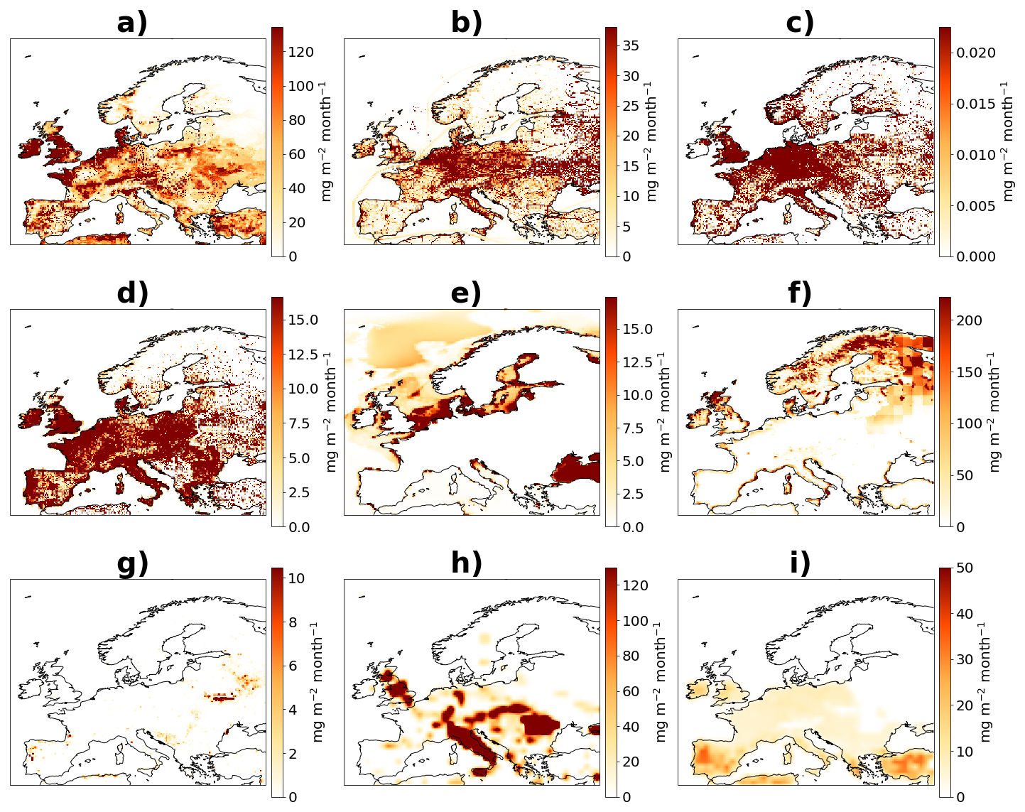
Figure A1Mean spatial distribution of prior methane (CH4) fluxes over the inversion domain for 2017–2022. Prior emissions are shown by sector: (a) Agriculture (AGR), (b) Energy (ENG), (c) Industrial processes (IND), (d) Waste (WST), (e) Ocean (OCE), (f) Wetlands and soil sinks (WET), (g) Biomass burning (BBR), (h) Geological (GEO), and (i) Termites (TER). Anthropogenic prior fluxes were derived monthly from GAINS (for EU27+3) and EDGARv8 (for the rest of the world). The GAINS sectors contributing to the AGR, ENG, and WST categories include: Energy: A_PublicPower, B_Industry, D_Fugitives, F_RoadTransport, C_OtherStationaryComb; Agriculture: K_AgriLivestock, L_AgriOther; Waste: J_Waste. The EDGARv8 sectoral inputs correspond to IPCC categories: Energy: BUILDINGS, TRANSPORT, IND_COMBUSTION, POWER_INDUSTRY, FUEL_EXPLOITATION; Industrial processes: IND_PROCESSES; Agriculture; AGRICULTURE; Waste: WASTE.
Table A1Subregional grouping of European countries used in this study. ISO codes follow ISO 3166-1 alpha-3.
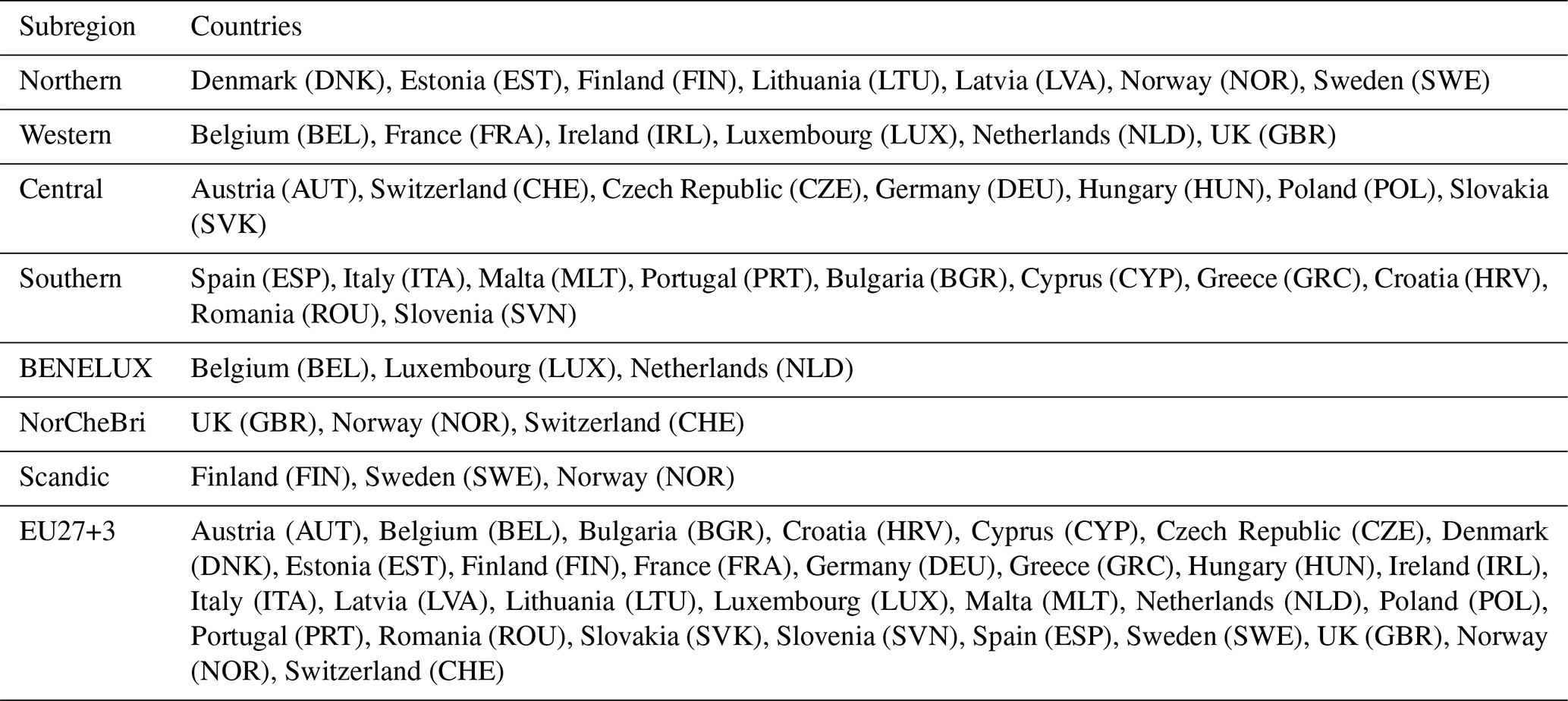
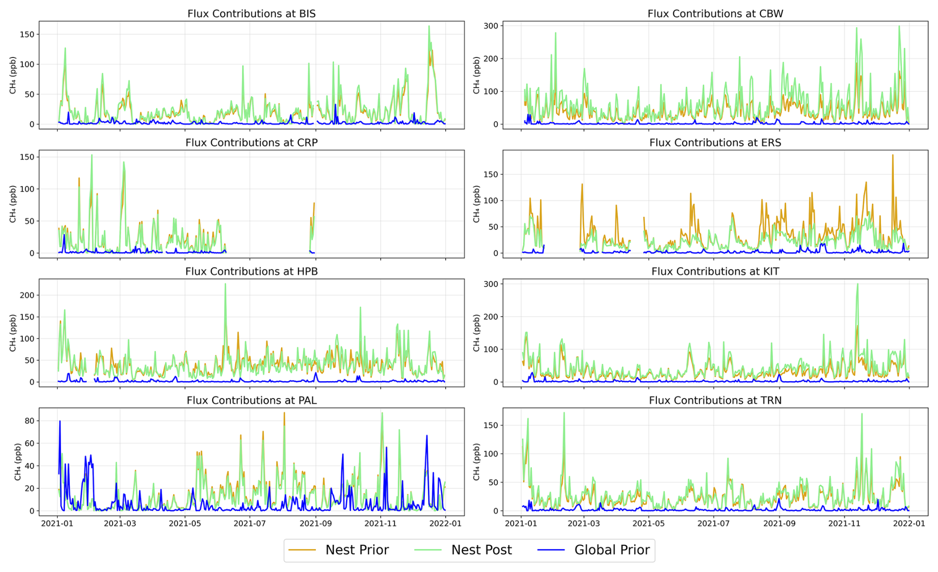
Figure A2Time series of CH4 flux contributions from the nested and global domains at selected stations, averaged at the assimilated hour for 2021: BIS (Biscarrosse, France), CBW (Cabauw, Netherlands), CRP (Carnsore Point, Ireland), ERS (Ersa, coastal Mediterranean site), HPB (Hohenpeissenberg, mountain station in Germany), KIT (Karlsruhe, Germany), PAL (Pallas, Finland), and TRN (Trainou, France).
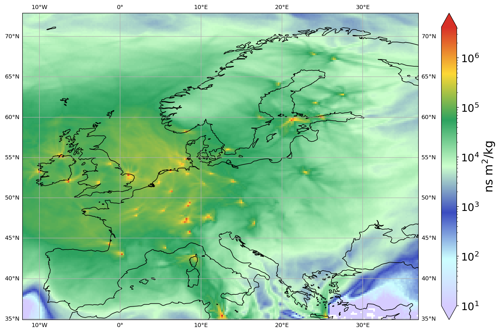
Figure A3FLEXPART footprint sensitivity to the assimilated observations, shown as the mean sensitivity field for July 2021, illustrating the spatial heterogeneity of observational constraints across Europe. Regions with denser measurement coverage exhibit stronger sensitivities.
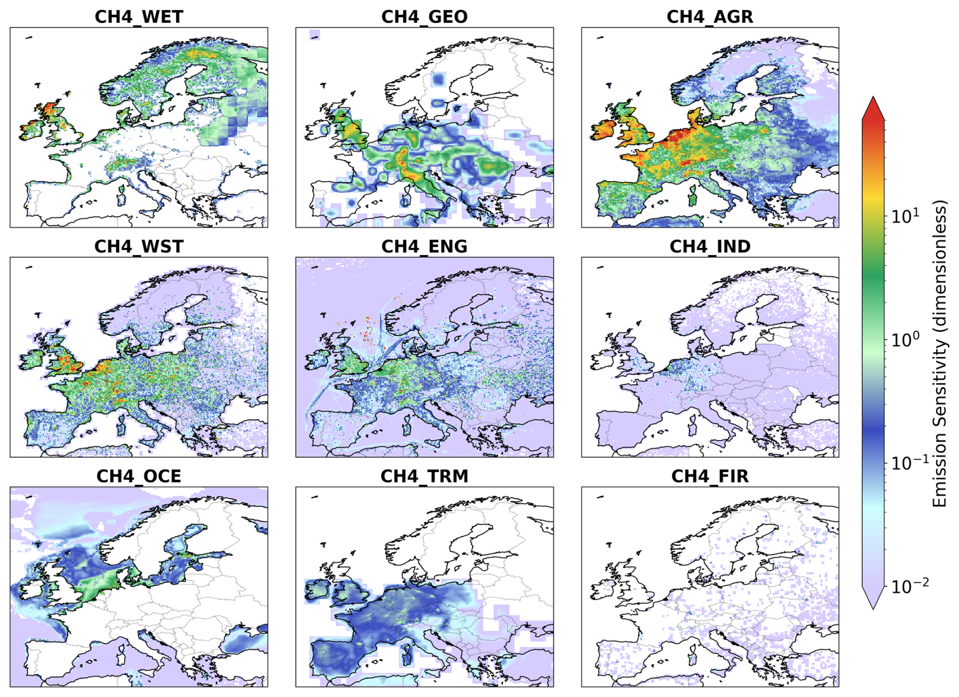
Figure A4Emission sensitivity, defined as the product of the footprint sensitivity and the monthly mean prior CH4 flux for each emission sector, indicating where prior emissions and observational sensitivity jointly contribute to constraining the inversion.
Table A2List of CH4 concentration observation sites assimilated in this study. The “Alt” represents the sum of the surface elevation and the intake height a.g.l.. The “Usage” column uses “M” to denote stations included in the base inversion and “S” to denote stations used only in the sensitivity test. An asterisk (*) in the three-letter station code indicates the station is classified as a mountain station, while a double asterisk (**) indicates the station is classified as a coastal station. Time series of CH4 concentration are obtained from the ICOS European ObsPack compilation, except for SOD and KMP, which are provided by FMI.
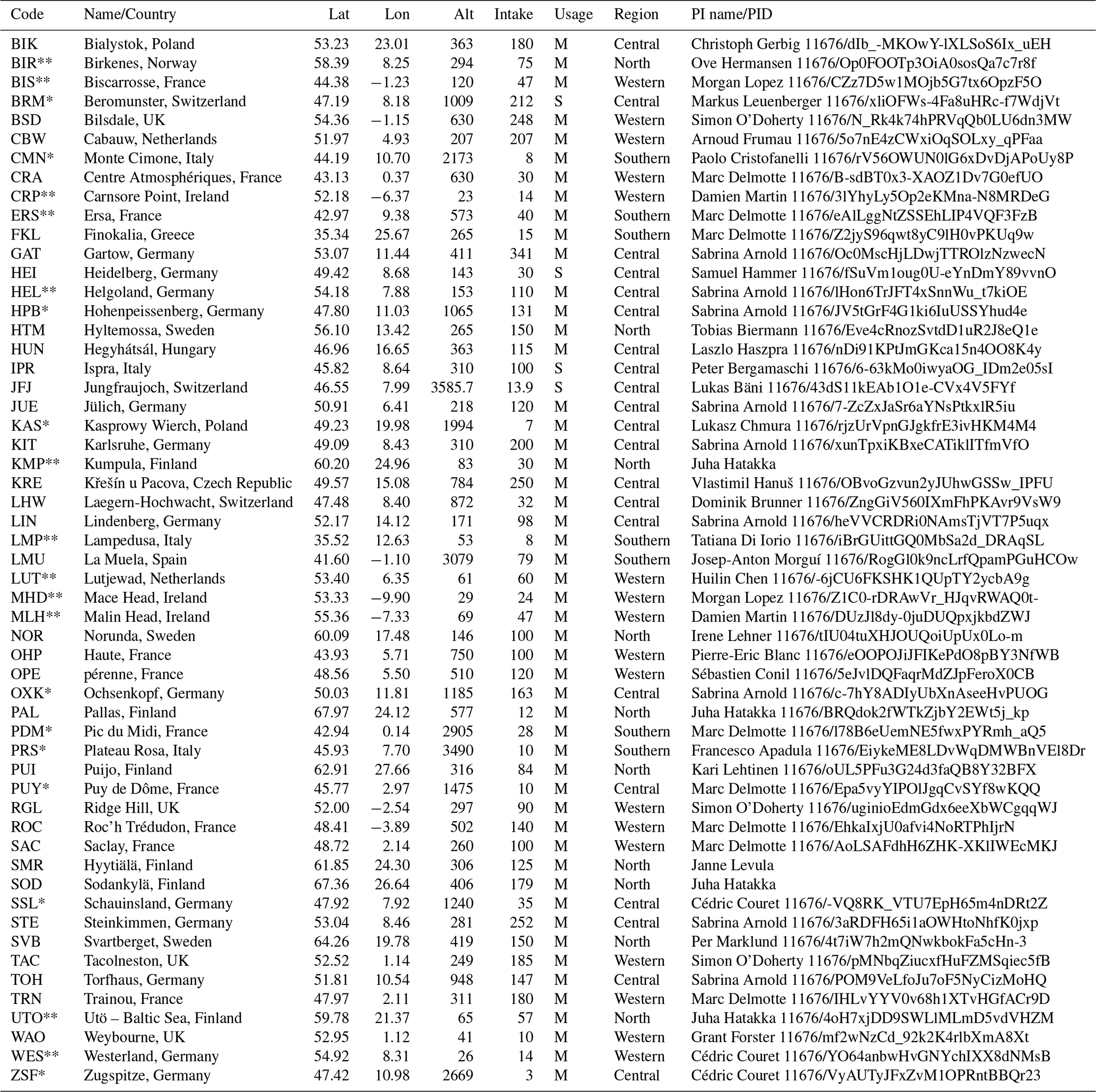
All links were accessed on 20 June 2026.
Table A3Prior and posterior model performance statistics at all measurement stations used in this study. The table reports the root-mean-square error (RMSE), mean bias (MBias), and Pearson correlation coefficient (r2) for both the prior and posterior simulations at the assimilated hour. RMSE and MBias are given in ppb.
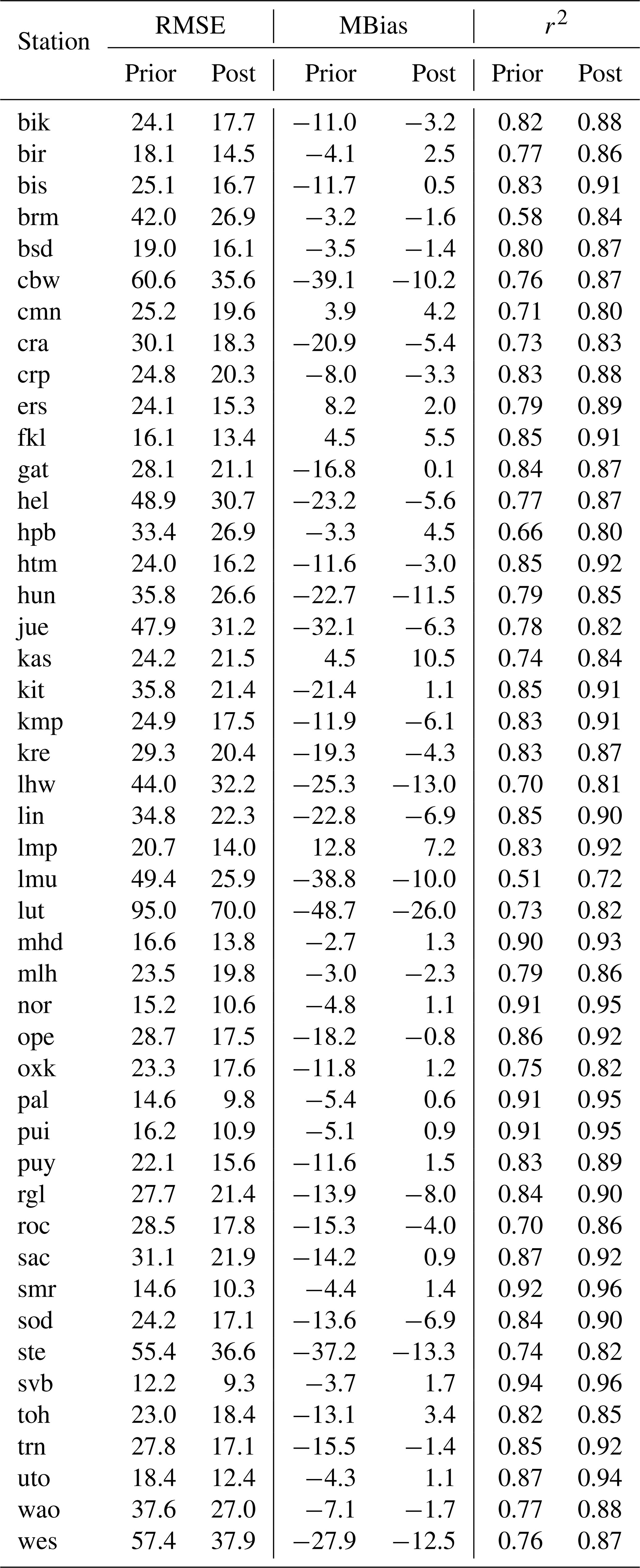
Table A4Six-year mean methane fluxes (2017–2022) by region and sector. Values are given in Tg yr−1 with ranges in parentheses.
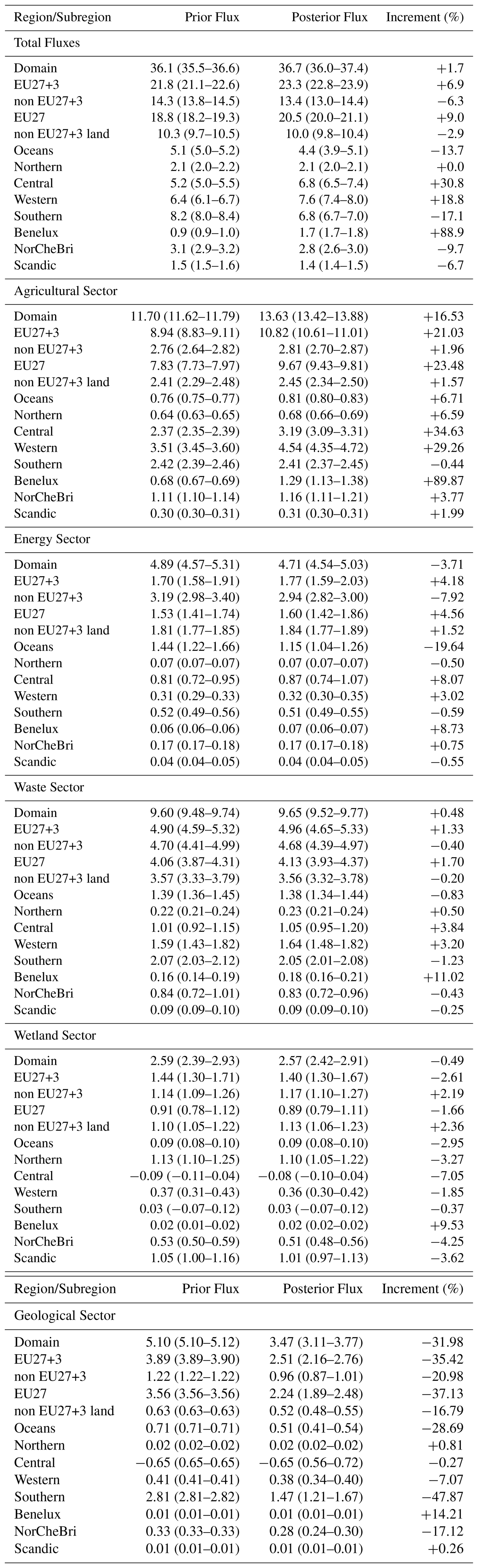
Table A5Comparison of posterior anthropogenic CH4 emissions (Tg yr−1) for EU27+3 countries with GAINS, UNFCCC, and EDGARv8 inventories, including relative differences (%).
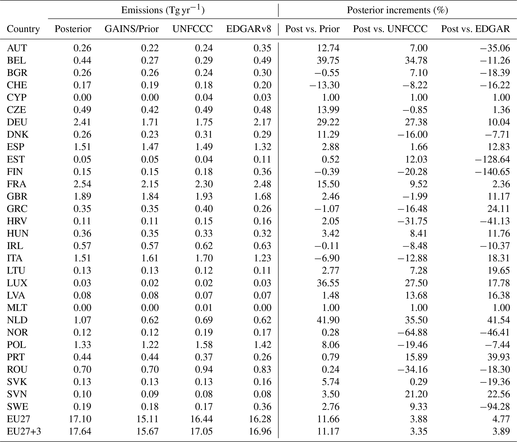
This study makes use of the Community Inversion Framework (CIF; Berchet et al., 2021a) and the Lagrangian transport model FLEXPART v10.4 (Pisso et al., 2019). The CIF code, documentation, and demonstration data are available at https://doi.org/10.5281/zenodo.5045730 (Berchet et al., 2021b). FLEXPART v10.4 is publicly available at https://gitlab.phaidra.org/flexpart/flexpart/-/releases/v10.4, last access: 20 June 2026.
The time series of CH4 dry air mole fraction data used in this study are available from the Integrated Carbon Observation System (ICOS) at https://www.icos-cp.eu/ (last access: 23 June 2026) obspack_CH4_466_GVeu_v10.0_20240729 European CH4. Prior emission inventories were obtained from publicly available sources: GAINS (https://iiasa.ac.at/web/home/research/researchPrograms/air/GAINS.html last access: 30 July 2026, EDGARv8 (https://edgar.jrc.ec.europa.eu/, last access: 30 October 2025, and JSBACH-HIMMELI (available upon request from the model developers). Climatological emissions from geological, oceanic, and termite sources follow published datasets cited in this study. Data used for plotting the results of this study will be made available on Zenodo following final publication.
AGM, AT, and TA conceived and designed the study and coordinated the analysis. AGM conducted the inversion runs and prepared the visualisations. AB, AM, AFC, and RT developed the CIF-FLEXPART framework and supported model setup. AGM drafted the manuscript with substantial input from AT, HL, and TA. AGM, AT, TM, and TA collected and processed the observational and prior data. ALe and MT ran the JSBACH–HIMMELI model and provided the wetland CH4 emission estimates. LHI provided the GAINS CH4 emissions. ALa contributed methane observations, processing, and analysis. TA and HL provided supervision and resources. All authors contributed to interpreting the results, participated in the scientific discussion, and reviewed and approved the final manuscript.
The contact author has declared that none of the authors has any competing interests.
Publisher's note: Copernicus Publications remains neutral with regard to jurisdictional claims made in the text, published maps, institutional affiliations, or any other geographical representation in this paper. The authors bear the ultimate responsibility for providing appropriate place names. Views expressed in the text are those of the authors and do not necessarily reflect the views of the publisher.
We thank the developers and maintainers of the Community Inversion Framework (CIF) and FLEXPART for making their models openly available. We acknowledge the providers of the emission inventories used in this study, including GAINS, EDGARv8, GFED, JSBACH-HIMMELI, and the LPX-Bern DYPTOP v1.4 model for global biospheric emissions. We also thank the European Centre for Medium-Range Weather Forecasts (ECMWF) for providing meteorological data and the Copernicus Atmosphere Monitoring Service (CAMS) for providing background mole fraction data. The authors would like to thank the ICOS and non-ICOS Principal Investigators (PIs) for providing high-quality CH4 mole-fraction observations (ICOS RI et al., 2023). We acknowledge the PIs and technical teams of the ICOS and non-ICOS stations contributing data to this study (the list of PIs, stations, and PIDs is provided in Appendix A, Table A2). The CH4 mole fraction data were sourced from the ICOS Carbon Portal: https://doi.org/10.18160/9CQ4-W69K (ICOS RI et al., 2023). We thank the Finnish Meteorological Institute for KMP and SOD observations. We also thank colleagues and collaborators for valuable discussions that improved this work, and we are grateful to Tianqi Shi for providing the country mask. We are also grateful to CSC–IT Center for Science, Finland, for providing the high-performance computing resources. We acknowledge the use of AI-assisted tools such as Grammarly and ChatGPT (OpenAI) for improving the language and clarity of the manuscript. We would also like to thank the Associate Editor Jason West and the anonymous reviewers for their constructive and thoughtful comments and suggestions, which significantly improved the manuscript.
This research has been supported by the Research Council of Finland (RCF-GHGSUPER, grant no. 351311; RCF-CHARM, grant no. 364975; RCF Flagships ACCC and FAME, grant nos. 337552 and 359196; WINMET, grant no. 350184; and FIRI-ICOS Finland, grant no. 345531), the EU Horizon Europe Climate, Energy and Mobility programme (EYE-CLIMA and IM4CA, grant nos. 101081395 and 101183460), Business Finland (BF-AGCLIMATE), and VNK-HIKET.
This paper was edited by Jason West and reviewed by two anonymous referees.
Aalto, T., Tsuruta, A., Mäkelä, J., Müller, J., Tenkanen, M., Burke, E., Chadburn, S., Gao, Y., Mannisenaho, V., Kleinen, T., Lee, H., Leppänen, A., Markkanen, T., Materia, S., Miller, P. A., Peano, D., Peltola, O., Poulter, B., Raivonen, M., Saunois, M., Wårlind, D., and Zaehle, S.: Air temperature and precipitation constraining the modelled wetland methane emissions in a boreal region in northern Europe, Biogeosciences, 22, 323–340, https://doi.org/10.5194/bg-22-323-2025, 2025. a
Bechtold, E. K., Ellenbogen, J. B., Villa, J. A., de Melo Ferreira, D. K., Oliverio, A. M., Kostka, J. E., Rich, V. I., Varner, R. K., Bansal, S., Ward, E. J., Bohrer, G., Borton, M. A., Wrighton, K. C., and Wilkins, M. J.: Metabolic interactions underpinning high methane fluxes across terrestrial freshwater wetlands, Nat. Commun., 16, 944, https://doi.org/10.1038/s41467-025-56133-0, 2025. a
Berchet, A., Sollum, E., Thompson, R. L., Pison, I., Thanwerdas, J., Broquet, G., Chevallier, F., Aalto, T., Berchet, A., Bergamaschi, P., Brunner, D., Engelen, R., Fortems-Cheiney, A., Gerbig, C., Groot Zwaaftink, C. D., Haussaire, J.-M., Henne, S., Houweling, S., Karstens, U., Kutsch, W. L., Luijkx, I. T., Monteil, G., Palmer, P. I., van Peet, J. C. A., Peters, W., Peylin, P., Potier, E., Rödenbeck, C., Saunois, M., Scholze, M., Tsuruta, A., and Zhao, Y.: The Community Inversion Framework v1.0: a unified system for atmospheric inversion studies, Geosci. Model Dev., 14, 5331–5354, https://doi.org/10.5194/gmd-14-5331-2021, 2021a. a, b
Berchet, A., Sollum, E., Pison, I., Thompson, R. L., Thanwerdas, J., Fortems-Cheiney, A., van Peet, J. C. A., Potier, E., Chevallier, F., Broquet, G., and Berchet, A.: The Community Inversion Framework: codes and documentation, Zenodo [software], https://doi.org/10.5281/zenodo.5045730, 2021b. a
Bergamaschi, P., Houweling, S., Segers, A., Krol, M., Frankenberg, C., Scheepmaker, R. A., Dlugokencky, E., Wofsy, S. C., Kort, E. A., Sweeney, C., Schuck, T., Brenninkmeijer, C., Chen, H., Beck, V., and Gerbig, C.: Atmospheric CH4 in the first decade of the 21st century: inverse modeling analysis using SCIAMACHY satellite retrievals and NOAA surface measurements, J. Geophys. Res.-Atmos., 118, 7350–7369, https://doi.org/10.1002/jgrd.50480, 2013. a
Bergamaschi, P., Corazza, M., Karstens, U., Athanassiadou, M., Thompson, R. L., Pison, I., Manning, A. J., Bousquet, P., Segers, A., Vermeulen, A. T., Janssens-Maenhout, G., Schmidt, M., Ramonet, M., Meinhardt, F., Aalto, T., Haszpra, L., Moncrieff, J., Popa, M. E., Lowry, D., Steinbacher, M., Jordan, A., O'Doherty, S., Piacentino, S., and Dlugokencky, E.: Top-down estimates of European CH4 and N2O emissions based on four different inverse models, Atmos. Chem. Phys., 15, 715–736, https://doi.org/10.5194/acp-15-715-2015, 2015. a
Bergamaschi, P., Segers, A., Brunner, D., Haussaire, J.-M., Henne, S., Ramonet, M., Arnold, T., Biermann, T., Chen, H., Conil, S., Delmotte, M., Forster, G., Frumau, A., Kubistin, D., Lan, X., Leuenberger, M., Lindauer, M., Lopez, M., Manca, G., Müller-Williams, J., O'Doherty, S., Scheeren, B., Steinbacher, M., Trisolino, P., Vítková, G., and Yver Kwok, C.: High-resolution inverse modelling of European CH4 emissions using the novel FLEXPART-COSMO TM5 4DVAR inverse modelling system, Atmos. Chem. Phys., 22, 13243–13268, https://doi.org/10.5194/acp-22-13243-2022, 2022. a, b, c, d, e, f
Bocquet, M. and Sakov, P.: Joint state and parameter estimation with an iterative ensemble Kalman smoother, Nonlin. Processes Geophys., 20, 803–818, https://doi.org/10.5194/npg-20-803-2013, 2013. a, b
Cael, B. and Goodwin, P.: Global methane pledge versus carbon dioxide emission reduction, Environ. Res. Lett., 18, 104015, https://doi.org/10.1088/1748-9326/acf8dd, 2023. a
Chen, Z., Jacob, D. J., Nesser, H., Sulprizio, M. P., Lorente, A., Varon, D. J., Lu, X., Shen, L., Qu, Z., Penn, E., and Yu, X.: Methane emissions from China: a high-resolution inversion of TROPOMI satellite observations, Atmos. Chem. Phys., 22, 10809–10826, https://doi.org/10.5194/acp-22-10809-2022, 2022. a, b, c
Crippa, M., Solazzo, E., Huang, G., Guizzardi, D., Koffi, E., Muntean, M., Schieberle, C., Friedrich, R., and Janssens-Maenhout, G.: High resolution temporal profiles in the emissions database for global atmospheric research, Scientific Data, 7, 121, https://doi.org/10.1038/s41597-020-0462-2, 2020. a
Dlugokencky, E. J., Nisbet, E. G., Fisher, R., and Lowry, D.: Global atmospheric methane: budget, changes and dangers, Philos. T. Roy. Soc. A, 369, 2058–2072, https://doi.org/10.1098/rsta.2010.0341, 2011. a
East, J. D., Jacob, D. J., Jervis, D., Balasus, N., Estrada, L. A., Hancock, S. E., Sulprizio, M. P., Thomas, J., Wang, X., Chen, Z., Varon, D. J., and Worden, J. R.: Worldwide inference of national methane emissions by inversion of satellite observations with UNFCCC prior estimates, Nat. Commun., 16, 11004, https://doi.org/10.1038/s41467-025-67122-8, 2025. a
Ernst, Y., Archibald, S., Balzter, H., Chevallier, F., Ciais, P., Gonzalez Fischer, C., Gaubert, B., Higginbottom, T., Higgins, S., Lawal, S., Lacroix, F., Lauerwald, R., Lourenco, M., Martens, C., Mengistu, A. G., Merbold, L., Mitchard, E., Moyo, M., Nguyen, H., O’Sullivan, M., Rodríguez-Veiga, P., Rosan, T., Rosentreter, J., Ryan, C., Scheiter, S., Sitch, S., Stevens, N., Tagesson, T., Tian, H., Wang, M., Woon, J. S., Zheng, B., Zhou, Y., and Scholes, R. J.: The African regional greenhouse gases budget (2010–2019), Global Biogeochem. Cy., 38, e2023GB008016, https://doi.org/10.1029/2023GB008016, 2024. a
Etiope, G., Ciotoli, G., Schwietzke, S., and Schoell, M.: Gridded maps of geological methane emissions and their isotopic signature, Earth Syst. Sci. Data, 11, 1–22, https://doi.org/10.5194/essd-11-1-2019, 2019. a
Friedlingstein, P., O'Sullivan, M., Jones, M. W., Andrew, R. M., Gregor, L., Hauck, J., Le Quéré, C., Luijkx, I. T., Olsen, A., Peters, G. P., Peters, W., Pongratz, J., Schwingshackl, C., Sitch, S., Canadell, J. G., Ciais, P., Jackson, R. B., Alin, S. R., Alkama, R., Arneth, A., Arora, V. K., Bates, N. R., Becker, M., Bellouin, N., Bittig, H. C., Bopp, L., Chevallier, F., Chini, L. P., Cronin, M., Evans, W., Falk, S., Feely, R. A., Gasser, T., Gehlen, M., Gkritzalis, T., Gloege, L., Grassi, G., Gruber, N., Gürses, Ö., Harris, I., Hefner, M., Houghton, R. A., Hurtt, G. C., Iida, Y., Ilyina, T., Jain, A. K., Jersild, A., Kadono, K., Kato, E., Kennedy, D., Klein Goldewijk, K., Knauer, J., Korsbakken, J. I., Landschützer, P., Lefèvre, N., Lindsay, K., Liu, J., Liu, Z., Marland, G., Mayot, N., McGrath, M. J., Metzl, N., Monacci, N. M., Munro, D. R., Nakaoka, S.-I., Niwa, Y., O'Brien, K., Ono, T., Palmer, P. I., Pan, N., Pierrot, D., Pocock, K., Poulter, B., Resplandy, L., Robertson, E., Rödenbeck, C., Rodriguez, C., Rosan, T. M., Schwinger, J., Séférian, R., Shutler, J. D., Skjelvan, I., Steinhoff, T., Sun, Q., Sutton, A. J., Sweeney, C., Takao, S., Tanhua, T., Tans, P. P., Tian, X., Tian, H., Tilbrook, B., Tsujino, H., Tubiello, F., van der Werf, G. R., Walker, A. P., Wanninkhof, R., Whitehead, C., Willstrand Wranne, A., Wright, R., Yuan, W., Yue, C., Yue, X., Zaehle, S., Zeng, J., and Zheng, B.: Global Carbon Budget 2022, Earth Syst. Sci. Data, 14, 4811–4900, https://doi.org/10.5194/essd-14-4811-2022, 2022. a
Gaspari, G. and Cohn, S. E.: Construction of correlation functions in two and three dimensions, Q. J. Roy. Meteor. Soc., 125, 723–757, https://doi.org/10.1002/qj.49712555417, 1999. a, b
Gilbert, J. C. and Lemaréchal, C.: The module M1QN3, Technical report, INRIA Rocquencourt, Domaine de Voluceau, BP 105, 78153 Le Chesnay Cedex, France, https://inria.hal.science/hal-04146287/document (last access: 30 October 2025), 2009. a
Hazan, L., Tarniewicz, J., Ramonet, M., Laurent, O., and Abbaris, A.: Automatic processing of atmospheric CO2 and CH4 mole fractions at the ICOS Atmosphere Thematic Centre, Atmos. Meas. Tech., 9, 4719–4736, https://doi.org/10.5194/amt-9-4719-2016, 2016. a
Hu, L., Andrews, A. E., Montzka, S. A., Miller, S. M., Bruhwiler, L., Oh, Y., Sweeney, C., Miller, J. B., McKain, K., Ibarra Espinosa, S., Davis, K., Miles, N., Mountain, M., Lan, X., Crotwell, A., Madronich, M., Mefford, T., Michel, S., and Houweling, S.: An unexpected seasonal cycle in U.S. oil and gas methane emissions, Environ. Sci. Technol., 59, 9968–9979, https://doi.org/10.1021/acs.est.4c14090, 2025. a
Höglund-Isaksson, L., Gómez-Sanabria, A., Klimont, Z., Rafaj, P., and Schöpp, W.: Technical potentials and costs for reducing global anthropogenic methane emissions in the 2050 timeframe – results from the GAINS model, Environmental Research Communications, 2, 025004, https://doi.org/10.1088/2515-7620/ab7457, 2020. a
ICOS RI, Bergamaschi, P., Colomb, A., De Mazière, M., Emmenegger, L., Kubistin, D., Lehner, I., Lehtinen, K., Lund Myhre, C., Marek, M., O'Doherty, S., Platt, S. M., Plaß-Dülmer, C., Ramonet, M., Apadula, F., Arnold, S., Blanc, P.-E., Brunner, D., Chen, H., Chmura, L., Conil, S., Couret, C., Cristofanelli, P., Delmotte, M., Forster, G., Frumau, A., Gheusi, F., Hammer, S., Haszpra, L., Hatakka, J., Heliasz, M., Henne, S., Hoheisel, A., Kneuer, T., Laurila, T., Leskinen, A., Leuenberger, M., Levin, I., Lindauer, M., Lunder, C., Mammarella, I., Manca, G., Manning, A., Martin, D., Meinhardt, F., Mölder, M., Müller-Williams, J., Necki, J., Ottosson-Löfvenius, M., Philippon, C., Piacentino, S., Pitt, J., Rivas-Soriano, P., Scheeren, B., Schumacher, M., Sha, M. K., Smith, P., Spain, G., Steinbacher, M., Sørensen, L. L., Vermeulen, A., Vítková, G., Xueref-Remy, I., di Sarra, A., Conen, F., Kazan, V., Roulet, Y.-A., Biermann, T., Heltai, D., Hensen, A., Hermansen, O., Komínková, K., Laurent, O., Levula, J., Lopez, M., Marklund, P., Pichon, J.-M., Schmidt, M., Stanley, K., Trisolino, P., ICOS Carbon Portal, ICOS Atmosphere Thematic Centre, ICOS Flask And Calibration Laboratory, and ICOS Central Radiocarbon Laboratory: European Obspack compilation of atmospheric methane data from ICOS and non-ICOS European stations for the period 1984–2023; obspack_ch4_466_GVeu_20230913, ICOS ERIC – Carbon Portal [data set], https://doi.org/10.18160/9CQ4-W69K, 2023. a, b, c, d
Ioannidis, E., Meesters, A., Steiner, M., Brunner, D., Reum, F., Pison, I., Berchet, A., Thompson, R., Sollum, E., Koch, F.-T., Gerbig, C., Wang, F., Maksyutov, S., Tsuruta, A., Tenkanen, M., Aalto, T., Monteil, G., Lin, H., Ren, G., Scholze, M., and Houweling, S.: An inter-comparison of inverse models for estimating European CH4 emissions, Earth Syst. Sci. Data, 18, 167–198, https://doi.org/10.5194/essd-18-167-2026, 2026. a, b
IPCC: 2006 IPCC Guidelines for National Greenhouse Gas Inventories, IPCC Guidelines, https://www.ipcc-nggip.iges.or.jp/public/2006gl/ (last access: November 2025), 2006. a
IPCC: Refinement to the 2006 IPCC guidelines for national greenhouse gas inventories, IPCC Guidelines for National Greenhouse Gas Inventories, 3, report, https://www.ipcc-nggip.iges.or.jp/public/2019rf/vol5.html (last access: November 2025), 2019. a
IPCC: Climate Change 2021: The Physical Science Basis. Contribution of Working Group I to the Sixth Assessment Report of the Intergovernmental Panel on Climate Change, edited by: Masson-Delmotte, V., Zhai, P., Pirani, A., Connors, S. L., Péan, C., Berger, S., Caud, N., Chen, Y., Goldfarb, L., Gomis, M. I., and others, Cambridge University Press, Cambridge, UK and New York, NY, USA, https://doi.org/10.1017/9781009157896, 2023a. a
IPCC: Climate Change 2023: Synthesis Report of the IPCC Sixth Assessment Report (AR6), IPCC Report, https://www.ipcc.ch/report/ar6/syr/ (last access: November 2025), 2023b. a
Kikstra, J. S., Nicholls, Z. R. J., Smith, C. J., Lewis, J., Lamboll, R. D., Byers, E., Sandstad, M., Meinshausen, M., Gidden, M. J., Rogelj, J., Kriegler, E., Peters, G. P., Fuglestvedt, J. S., Skeie, R. B., Samset, B. H., Wienpahl, L., van Vuuren, D. P., van der Wijst, K.-I., Al Khourdajie, A., Forster, P. M., Reisinger, A., Schaeffer, R., and Riahi, K.: The IPCC Sixth Assessment Report WGIII climate assessment of mitigation pathways: from emissions to global temperatures, Geosci. Model Dev., 15, 9075–9109, https://doi.org/10.5194/gmd-15-9075-2022, 2022. a
Krol, M., Houweling, S., Bregman, B., van den Broek, M., Segers, A., van Velthoven, P., Peters, W., Dentener, F., and Bergamaschi, P.: The two-way nested global chemistry-transport zoom model TM5: algorithm and applications, Atmos. Chem. Phys., 5, 417–432, https://doi.org/10.5194/acp-5-417-2005, 2005. a
Leip, A., Skiba, U., Vermeulen, A., and Thompson, R. L.: A complete rethink is needed on how greenhouse gas emissions are quantified for national reporting, Atmos. Environ., 174, 237–240, https://doi.org/10.1016/j.atmosenv.2017.12.006, 2018. a
Lienert, S. and Joos, F.: A Bayesian ensemble data assimilation to constrain model parameters and land-use carbon emissions, Biogeosciences, 15, 2909–2930, https://doi.org/10.5194/bg-15-2909-2018, 2018. a
Mikaloff Fletcher, S. E., Tans, P. P., Bruhwiler, L. M., Miller, J. B., and Heimann, M.: CH4 sources estimated from atmospheric observations of CH4 and its isotopic ratios: 1. Inverse modeling of source processes, Global Biogeochem. Cy., 18, https://doi.org/10.1029/2004GB002223, 2004. a
Monteiro, V. C., Turnbull, J. C., Miles, N. L., Davis, K. J., Barkley, Z., and Deng, A.: Assimilating morning, evening, and nighttime greenhouse gas observations in atmospheric inversions, J. Geophys. Res.-Atmos., 129, e2024JD040998, https://doi.org/10.1029/2024JD040998, 2024. a
Myhre, G., Shindell, D., Bréon, F.-M., Collins, W., Fuglestvedt, J., Huang, J., Koch, D., Lamarque, J.-F., Lee, D., Mendoza, B., Nakajima, T., Robock, A., Stephens, G., Takemura, T., and Zhang, H.: Anthropogenic and natural radiative forcing, in: Climate Change 2013: The Physical Science Basis. Contribution of Working Group I to the Fifth Assessment Report of the Intergovernmental Panel on Climate Change, edited by: Stocker, T. F., Qin, D., Plattner, G.-K., Tignor, M., Allen, S. K., Boschung, J., Nauels, A., Xia, Y., Bex, V., and Midgley, P. M., chapter in IPCC AR5, Cambridge University Press, Cambridge, UK and New York, NY, USA, https://www.ipcc.ch/report/ar5/wg1/ (last access: 30 October 2025), 2013. a
Peltola, O., Hensen, A., Belelli Marchesini, L., Helfter, C., Bosveld, F. C., van den Bulk, W. C. M., Haapanala, S., van Huissteden, J., Laurila, T., Lindroth, A., Nemitz, E., Röckmann, T., Vermeulen, A. T., and Mammarella, I.: Studying the spatial variability of methane flux with five eddy covariance towers of varying height, Agr. Forest Meteorol., 214–215, 456–472, https://doi.org/10.1016/j.agrformet.2015.09.007, 2015. a
Peters, W., Miller, J. B., Whitaker, J., Denning, A. S., Hirsch, A., Krol, M. C., Zupanski, D., Bruhwiler, L., and Tans, P. P.: An ensemble data assimilation system to estimate CO2 surface fluxes from atmospheric trace gas observations, J. Geophys. Res.-Atmos., 110, https://doi.org/10.1029/2005JD006157, 2005. a, b
Petrescu, A. M. R., Qiu, C., Ciais, P., Thompson, R. L., Peylin, P., McGrath, M. J., Solazzo, E., Janssens-Maenhout, G., Tubiello, F. N., Bergamaschi, P., Brunner, D., Peters, G. P., Höglund-Isaksson, L., Regnier, P., Lauerwald, R., Bastviken, D., Tsuruta, A., Winiwarter, W., Patra, P. K., Kuhnert, M., Oreggioni, G. D., Crippa, M., Saunois, M., Perugini, L., Markkanen, T., Aalto, T., Groot Zwaaftink, C. D., Tian, H., Yao, Y., Wilson, C., Conchedda, G., Günther, D., Leip, A., Smith, P., Haussaire, J.-M., Leppänen, A., Manning, A. J., McNorton, J., Brockmann, P., and Dolman, A. J.: The consolidated European synthesis of CH4 and N2O emissions for the European Union and United Kingdom: 1990–2017, Earth Syst. Sci. Data, 13, 2307–2362, https://doi.org/10.5194/essd-13-2307-2021, 2021. a, b, c, d, e, f
Petrescu, A. M. R., Qiu, C., McGrath, M. J., Peylin, P., Peters, G. P., Ciais, P., Thompson, R. L., Tsuruta, A., Brunner, D., Kuhnert, M., Matthews, B., Palmer, P. I., Tarasova, O., Regnier, P., Lauerwald, R., Bastviken, D., Höglund-Isaksson, L., Winiwarter, W., Etiope, G., Aalto, T., Balsamo, G., Bastrikov, V., Berchet, A., Brockmann, P., Ciotoli, G., Conchedda, G., Crippa, M., Dentener, F., Groot Zwaaftink, C. D., Guizzardi, D., Günther, D., Haussaire, J.-M., Houweling, S., Janssens-Maenhout, G., Kouyate, M., Leip, A., Leppänen, A., Lugato, E., Maisonnier, M., Manning, A. J., Markkanen, T., McNorton, J., Muntean, M., Oreggioni, G. D., Patra, P. K., Perugini, L., Pison, I., Raivonen, M. T., Saunois, M., Segers, A. J., Smith, P., Solazzo, E., Tian, H., Tubiello, F. N., Vesala, T., van der Werf, G. R., Wilson, C., and Zaehle, S.: The consolidated European synthesis of CH4 and N2O emissions for the European Union and United Kingdom: 1990–2019, Earth Syst. Sci. Data, 15, 1197–1268, https://doi.org/10.5194/essd-15-1197-2023, 2023. a, b, c
Pisso, I., Sollum, E., Grythe, H., Kristiansen, N. I., Cassiani, M., Eckhardt, S., Arnold, D., Morton, D., Thompson, R. L., Groot Zwaaftink, C. D., Evangeliou, N., Sodemann, H., Haimberger, L., Henne, S., Brunner, D., Burkhart, J. F., Fouilloux, A., Brioude, J., Philipp, A., Seibert, P., and Stohl, A.: The Lagrangian particle dispersion model FLEXPART version 10.4, Geosci. Model Dev., 12, 4955–4997, https://doi.org/10.5194/gmd-12-4955-2019, 2019. a, b, c, d, e
Qu, Z., Jacob, D. J., Shen, L., Lu, X., Zhang, Y., Scarpelli, T. R., Nesser, H., Sulprizio, M. P., Maasakkers, J. D., Bloom, A. A., Worden, J. R., Parker, R. J., and Delgado, A. L.: Global distribution of methane emissions: a comparative inverse analysis of observations from the TROPOMI and GOSAT satellite instruments, Atmos. Chem. Phys., 21, 14159–14175, https://doi.org/10.5194/acp-21-14159-2021, 2021. a
Raivonen, M., Smolander, S., Backman, L., Susiluoto, J., Aalto, T., Markkanen, T., Mäkelä, J., Rinne, J., Peltola, O., Aurela, M., Lohila, A., Tomasic, M., Li, X., Larmola, T., Juutinen, S., Tuittila, E.-S., Heimann, M., Sevanto, S., Kleinen, T., Brovkin, V., and Vesala, T.: HIMMELI v1.0: HelsinkI Model of MEthane buiLd-up and emIssion for peatlands, Geosci. Model Dev., 10, 4665–4691, https://doi.org/10.5194/gmd-10-4665-2017, 2017. a
Ramonet, M., Ciais, P., Apadula, F., Bartyzel, J., Bastos, A., Bergamaschi, P., and Yver Kwok, C.: The fingerprint of the summer 2018 drought in Europe on ground-based atmospheric CO2 measurements, Philos. T. Roy. Soc. B, 375, https://doi.org/10.1098/rstb.2019.0513, 2020. a
Rayner, T. and Jordan, A.: Climate Change Policy in the European Union, https://doi.org/10.1093/acrefore/9780190228620.013.47, 2016. a
Reick, C. H., Gayler, V., Goll, D., Hagemann, S., Heidkamp, M., Nabel, J. E. M. S., Raddatz, T., Roeckner, E., Schnur, R., and Wilkenskjeld, S.: JSBACH 3 – The land component of the MPI Earth System Model: documentation of version 3.2, Tech. Rep. 240, Berichte zur Erdsystemforschung, https://doi.org/10.17617/2.3279802, 2021. a
Saunois, M., Stavert, A. R., Poulter, B., Bousquet, P., Canadell, J. G., Jackson, R. B., Raymond, P. A., Dlugokencky, E. J., Houweling, S., Patra, P. K., Ciais, P., Arora, V. K., Bastviken, D., Bergamaschi, P., Blake, D. R., Brailsford, G., Bruhwiler, L., Carlson, K. M., Carrol, M., Castaldi, S., Chandra, N., Crevoisier, C., Crill, P. M., Covey, K., Curry, C. L., Etiope, G., Frankenberg, C., Gedney, N., Hegglin, M. I., Höglund-Isaksson, L., Hugelius, G., Ishizawa, M., Ito, A., Janssens-Maenhout, G., Jensen, K. M., Joos, F., Kleinen, T., Krummel, P. B., Langenfelds, R. L., Laruelle, G. G., Liu, L., Machida, T., Maksyutov, S., McDonald, K. C., McNorton, J., Miller, P. A., Melton, J. R., Morino, I., Müller, J., Murguia-Flores, F., Naik, V., Niwa, Y., Noce, S., O'Doherty, S., Parker, R. J., Peng, C., Peng, S., Peters, G. P., Prigent, C., Prinn, R., Ramonet, M., Regnier, P., Riley, W. J., Rosentreter, J. A., Segers, A., Simpson, I. J., Shi, H., Smith, S. J., Steele, L. P., Thornton, B. F., Tian, H., Tohjima, Y., Tubiello, F. N., Tsuruta, A., Viovy, N., Voulgarakis, A., Weber, T. S., van Weele, M., van der Werf, G. R., Weiss, R. F., Worthy, D., Wunch, D., Yin, Y., Yoshida, Y., Zhang, W., Zhang, Z., Zhao, Y., Zheng, B., Zhu, Q., Zhu, Q., and Zhuang, Q.: The Global Methane Budget 2000–2017, Earth Syst. Sci. Data, 12, 1561–1623, https://doi.org/10.5194/essd-12-1561-2020, 2020. a, b, c, d, e, f, g
Saunois, M., Martinez, A., Poulter, B., Zhang, Z., Raymond, P. A., Regnier, P., Canadell, J. G., Jackson, R. B., Patra, P. K., Bousquet, P., Ciais, P., Dlugokencky, E. J., Lan, X., Allen, G. H., Bastviken, D., Beerling, D. J., Belikov, D. A., Blake, D. R., Castaldi, S., Crippa, M., Deemer, B. R., Dennison, F., Etiope, G., Gedney, N., Höglund-Isaksson, L., Holgerson, M. A., Hopcroft, P. O., Hugelius, G., Ito, A., Jain, A. K., Janardanan, R., Johnson, M. S., Kleinen, T., Krummel, P. B., Lauerwald, R., Li, T., Liu, X., McDonald, K. C., Melton, J. R., Mühle, J., Müller, J., Murguia-Flores, F., Niwa, Y., Noce, S., Pan, S., Parker, R. J., Peng, C., Ramonet, M., Riley, W. J., Rocher-Ros, G., Rosentreter, J. A., Sasakawa, M., Segers, A., Smith, S. J., Stanley, E. H., Thanwerdas, J., Tian, H., Tsuruta, A., Tubiello, F. N., Weber, T. S., van der Werf, G. R., Worthy, D. E. J., Xi, Y., Yoshida, Y., Zhang, W., Zheng, B., Zhu, Q., Zhu, Q., and Zhuang, Q.: Global Methane Budget 2000–2020, Earth Syst. Sci. Data, 17, 1873–1958, https://doi.org/10.5194/essd-17-1873-2025, 2025. a, b
Seibert, P. and Frank, A.: Source-receptor matrix calculation with a Lagrangian particle dispersion model in backward mode, Atmos. Chem. Phys., 4, 51–63, https://doi.org/10.5194/acp-4-51-2004, 2004. a
Shen, L., Jacob, D. J., Gautam, R., Omara, M., Scarpelli, T. R., Lorente, A., Zavala-Araiza, D., Lu, X., Chen, Z., and Lin, J.: National quantifications of methane emissions from fuel exploitation using high resolution inversions of satellite observations, Nat. Commun., 14, 4948, https://doi.org/10.1038/s41467-023-40671-6, 2023. a
Solazzo, E., Crippa, M., Guizzardi, D., Muntean, M., Choulga, M., and Janssens-Maenhout, G.: Uncertainties in the Emissions Database for Global Atmospheric Research (EDGAR) emission inventory of greenhouse gases, Atmos. Chem. Phys., 21, 5655–5683, https://doi.org/10.5194/acp-21-5655-2021, 2021. a
Steiner, M., Peters, W., Luijkx, I., Henne, S., Chen, H., Hammer, S., and Brunner, D.: European CH4 inversions with ICON-ART coupled to the CarbonTracker Data Assimilation Shell, Atmos. Chem. Phys., 24, 2759–2782, https://doi.org/10.5194/acp-24-2759-2024, 2024. a, b, c, d, e, f, g, h, i, j, k, l, m
Stohl, A., Wotawa, G., Seibert, P., and Kromp-Kolb, H.: Interpolation errors in wind fields as a function of spatial and temporal resolution and their impact on different types of kinematic trajectories, J. Appl. Meteorol., 34, 2149–2165, https://doi.org/10.1175/1520-0450(1995)034<2149:IEIWFA>2.0.CO;2, 1995. a, b, c
Szénási, B., Berchet, A., Broquet, G., Segers, A., van der Gon, H. D., Krol, M., Hullegie, J. J., Kiesow, A., Günther, D., Petrescu, A. M. R., Saunois, M., Bousquet, P., and Pison, I.: A pragmatic protocol for characterising errors in atmospheric inversions of methane emissions over Europe, Tellus B, 73, 1–23, https://doi.org/10.1080/16000889.2021.1914989, 2021. a
Tenkanen, M. K., Tsuruta, A., Denier van der Gon, H., Höglund-Isaksson, L., Leppänen, A., Markkanen, T., Petrescu, A. M. R., Raivonen, M., Aaltonen, H., and Aalto, T.: Partitioning anthropogenic and natural methane emissions in Finland during 2000–2021 by combining bottom-up and top-down estimates, Atmos. Chem. Phys., 25, 2181–2206, https://doi.org/10.5194/acp-25-2181-2025, 2025. a, b
Thompson, R. L. and Stohl, A.: FLEXINVERT: an atmospheric Bayesian inversion framework for determining surface fluxes of trace species using an optimized grid, Geosci. Model Dev., 7, 2223–2242, https://doi.org/10.5194/gmd-7-2223-2014, 2014. a, b, c, d
Tipka, A., Haimberger, L., and Seibert, P.: Flex_extract v7.1.2 – a software package to retrieve and prepare ECMWF data for use in FLEXPART, Geosci. Model Dev., 13, 5277–5310, https://doi.org/10.5194/gmd-13-5277-2020, 2020. a
Tsuruta, A., Aalto, T., Backman, L., Krol, M. C., Peters, W., Lienert, S., and Gomez-Pelaez, A. J.: Methane budget estimates in Finland from the CarbonTracker Europe-CH4 data assimilation system, Tellus B, 71, 1565030, https://doi.org/10.1080/16000889.2018.1565030, 2019. a
Tsuruta, A., Kivimäki, E., Lindqvist, H., Karppinen, T., Backman, L., Hakkarainen, J., Schneising, O., Buchwitz, M., Lan, X., Kivi, R., Chen, H., Buschmann, M., Herkommer, B., Notholt, J., Roehl, C., Té, Y., Wunch, D., Tamminen, J., and Aalto, T.: CH4 fluxes derived from assimilation of TROPOMI XCH4 in CarbonTracker Europe-CH4: evaluation of seasonality and spatial distribution in the northern high latitudes, Remote Sens.-Basel, 15, 1620, https://doi.org/10.3390/rs15061620, 2023. a
Turner, A. J., Frankenberg, C., and Kort, E. A.: Interpreting contemporary trends in atmospheric methane, P. Natl. Acad. Sci. USA, 116, 2805–2813, https://doi.org/10.1073/pnas.1814297116, 2019. a
van der Werf, G. R., Randerson, J. T., Giglio, L., van Leeuwen, T. T., Chen, Y., Rogers, B. M., Mu, M., van Marle, M. J. E., Morton, D. C., Collatz, G. J., Yokelson, R. J., and Kasibhatla, P. S.: Global fire emissions estimates during 1997–2016, Earth Syst. Sci. Data, 9, 697–720, https://doi.org/10.5194/essd-9-697-2017, 2017. a
Varon, D. J., Jacob, D. J., Estrada, L. A., Balasus, N., East, J. D., Pendergrass, D. C., Chen, Z., Sulprizio, M., Omara, M., Gautam, R., Barkley, Z. R., Cardoso Saldaña, F. J., Reidy, E. K., Kamdar, H., Sherwin, E. D., Biraud, S. C., Jervis, D., Pandey, S., Worden, J. R., Bowman, K. W., Maasakkers, J. D., and Kleinberg, R. L.: Seasonality and declining intensity of methane emissions from the Permian and nearby U.S. oil and gas basins, Environ. Sci. Technol., 60, 425–435, https://doi.org/10.1021/acs.est.5c08745, 2025. a
Vermeulen, A. T., Hensen, A., Popa, M. E., van den Bulk, W. C. M., and Jongejan, P. A. C.: Greenhouse gas observations from Cabauw Tall Tower (1992–2010), Atmos. Meas. Tech., 4, 617–644, https://doi.org/10.5194/amt-4-617-2011, 2011. a
Villani, M. G., Bergamaschi, P., Krol, M., Meirink, J. F., and Dentener, F.: Inverse modeling of European CH4 emissions: sensitivity to the observational network, Atmos. Chem. Phys., 10, 1249–1267, https://doi.org/10.5194/acp-10-1249-2010, 2010. a
Voigt, C., Virkkala, A.-M., Hould Gosselin, G., Bennett, K. A., Black, T. A., Detto, M., Chevrier-Dion, C., Guggenberger, G., Hashmi, W., Kohl, L., Kou, D., Marquis, C., Marsh, P., Marushchak, M. E., Nesic, Z., Nykänen, H., Saarela, T., Sauheitl, L., Walker, B., Weiss, N., Wilcox, E. J., and Sonnentag, O.: Arctic soil methane sink increases with drier conditions and higher ecosystem respiration, Nat. Clim. Change, 13, 1095–1104, https://doi.org/10.1038/s41558-023-01785-3, 2023. a
Weber, T., Wiseman, N. A., and Kock, A.: Global ocean methane emissions dominated by shallow coastal waters, Nat. Commun., 10, 4584, https://doi.org/10.1038/s41467-019-12541-7, 2019. a
WMO: Greenhouse Gas concentrations hit record high. Again., https://wmo.int/news/media-centre/greenhouse-gas-concentrations-hit-record-high-again (last access: November 2025), 2023. a