Introducing aerosol-cloud interactions in the ECMWF model reveals new constraints on aerosol representation

Realistic cloud droplet number concentrations (N_d) are critical for simulating the Earth's radiative budget, yet remain challenging to represent in global models. One reason is that aerosol optical depth (AOD), commonly used for aerosol validation and assimilation, only weakly constrains aerosol number concentrations relevant for cloud formation. We introduce a representation of aerosol-cloud interactions (ACI) into the ECMWF Integrated Forecasting System (IFS), restricted to aerosol activation and the first indirect effect, and use it as a diagnostic tool to relate aerosol properties to cloud observations in the Copernicus Atmosphere Monitoring System (CAMS). Using 18 years of MODIS N_d retrievals, we infer effective aerosol size distribution parameters and evaluate results using independent observations of AOD, Angstrom exponent, size spectra, and top-of-atmosphere shortwave fluxes. After optimisation, CAMS aerosols produce more realistic large-scale N_d patterns, but exhibit regional biases: overestimation over sub-Saharan Africa and underestimation at high latitudes. The African bias is consistent with carbonaceous aerosol emissions from wildfires and can be partially mitigated through optimisation, while the high-latitude bias is likely linked to excessive aerosol scavenging in mixed-phase clouds and cannot be resolved by size adjustments alone. We show that introducing phase-dependent aerosol scavenging substantially improves all-sky shortwave fluxes over the Southern Ocean compared to the ACI implementation in the standard CAMS system. This highlights a direct link between radiative biases and aerosol wet removal processes. Representing ACI in a weather model enables N_d to provide additional constraints on aerosol numbers and related processes globally, revealing limitations in how ageing, vertical transport and wet removal are represented, as these processes are only weakly constrained by standard AOD evaluation.

1 Introduction

The abundance of aerosols that act as cloud condensation nuclei (CCN) is a primary control on cloud droplet number concentrations (N_d) during cloud formation; N_d in turn determines the cloud droplet effective radius (r_e). Anthropogenic and natural changes in aerosols can thereby modify N_d and r_e, altering cloud albedo. This is referred to as the albedo (or Twomey) effect (Twomey, 1977, 1991) and represents the first, and best understood, of a cascade of aerosol indirect effects (Bellouin et al., 2020; Gordon et al., 2023) on the cloud droplet particle size distribution (PSD), with consequences on the cloud life cycle, macrophysics, and precipitation (Albrecht, 1989; Pincus and Baker, 1994). Such indirect effects are included under the umbrella term of aerosol-cloud interactions (ACI). Due to the macroscopic role of clouds in the regulation of the Earth's energy budget, ACI are considered necessary in global climate models to correctly capture the radiative response to anthropogenic aerosol emissions (Menon et al., 2002; Stier et al., 2005; Penner et al., 2006; Bellouin et al., 2011; Seinfeld et al., 2016; Mulcahy et al., 2018; Wang et al., 2021). However, such representations are still fraught with uncertainties, severely limiting the ability of models to predict climate change due to anthropogenic emissions (Szopa et al., 2023).

Activation of CCN into droplets is described by the Köhler theory (e.g. Pruppacher and Klett, 2010) for heterogeneous nucleation of cloud droplets. The efficiency of CCN in supporting droplet nucleation is controlled both by their solubility in water, and the amount of surface available for binding with water molecules. A popular way of describing CCN activation is in the form of the κ-Köhler theory (Petters and Kreidenweis, 2007), where aerosol chemical properties are condensed into a single hygroscopicity parameter κ (Quaas and Gryspeerdt, 2022). Since the early formulations by Twomey in the late 1950s, activation models have been developed that can accurately solve the equations derived by the κ-Köhler theory for the air parcel lifting condensation problem (see Ghan et al., 2011 for a detailed review). In addition, climate models employ computationally efficient parametrisations and lookup tables that have proven to perform satisfactorily compared to the full numerical models (Ghan et al., 2011).

Some numerical parametrisations can also represent activation of heterogenous aerosol mixtures and kinetic limitations of the activation process (Nenes et al., 2001; Ghan et al., 2011). These are needed to capture the effect of large sea salt particles on suppressing activation of available sulfate (${\mathrm{SO}}_{\mathrm{4}}^{\mathrm{2}-}$) aerosols for realistic aerosol populations and scenarios (Fossum et al., 2020). The relevance of this effect remains however unclear in actual atmospheric conditions, e.g. in terms of the regulation of the global energy budget or aerosol speciation itself. This could be explored, for instance, with more accurate representations of ACI in global models.

In the realm of global numerical weather prediction (NWP), models typically represent aerosol concentrations diagnostically using climatologies (e.g. Tegen et al., 1997; Bozzo et al., 2020). Such simplified descriptions allow the mean aerosol-radiation interaction to be captured while avoiding the computational cost of prognostic aerosol scheme simulations with tracer advection and interactions. A study by Mulcahy et al. (2014) showed that including indirect effects of prognostic aerosols has a widespread and potentially beneficial impact on the radiative budget of an NWP model. Ahlgrimm et al. (2018) showed that model biases in TOA shortwave (SW) radiative fluxes are dominated by errors in the cloud macrophysics (cloud cover, water phase, water content, and sub-grid heterogeneity) but also significantly affected by deficiencies in the cloud microphysics, indicating that those biases might be reduced by representing ACI. Furthermore, global NWP models have already started moving toward more complex two-moment cloud schemes (Field et al., 2023), where both water content and droplet number concentrations are prognostic variables; this direction implies an even higher importance of realistic CCN values for the cloud microphysics. Despite this, uncertainties in the physical processes involved in ACI and the difficulties in providing enough observational constraints (Rasch and Carslaw, 2022) have for a long time constituted a major challenge. However, the evolution of weather and climate forecasting systems towards more comprehensive Earth system representations, including air quality (Baklanov et al., 2017; Palmer et al., 2008), opens new opportunities for validating processes and representations. In addition to this, NWP models are thoroughly tested and monitored every day with a wide range of observations, which makes them an important test bed for ACI schemes. This offers the potential to refine these schemes in such a way that they can also inform climate models.

The Integrated Forecasting System (IFS) used at the European Centre for Medium-Range Weather Forecasts (ECMWF) is an NWP model used to perform operational global meteorological analyses and medium-range (10 d), sub-seasonal (42 d) and seasonal (4 months) forecasts. The IFS also supports an atmospheric-chemistry configuration denoted as IFS-COMPO (Flemming et al., 2015), with online chemistry and aerosol tracers, that is developed and maintained on behalf of the Copernicus Atmosphere Monitoring Service (CAMS). In the IFS-COMPO/CAMS configuration, a “bulk-bin” prognostic representation of aerosols is used (Rémy et al., 2022), but their feedback onto meteorological fields is only mediated by the direct radiative effect. The IFS currently diagnoses N_d for the calculation of r_e in liquid clouds using a wind-dependent parametrisation that differs between land and sea, but that has no dependence on either climatological or prognostic aerosols (ECMWF, 2024b). Similarly, the IFS uses fixed N_d values over land and sea for the calculation of cloud-to-rain water auto-conversion rates. Similar simplified descriptions have traditionally been used in NWP, but the increasing resolution of operational forecasts naturally leads to the demand for more realistic representations of aerosol-cloud interactions (Wilkinson et al., 2013).

Improving the representation of ACI in the IFS is a potential area of development at ECMWF, both for CAMS and NWP forecasts. ACI must also reflect the quality of the information provided by aerosol fields, either in a prognostic or climatological representation, the latter being used for forecasts on the medium-range (up to 10 d) and longer timescales (months). A recent study by Block et al. (2024) showed that the aerosols from the CAMS reanalysis (CAMSRA) can provide CCN diagnostics for validation against in-situ observations, but also revealed systematic errors hinting at underlying model issues. This illustrates the need for improved model aerosol descriptions to produce the most realistic possible global CCN concentrations and N_d values in liquid clouds, which constitutes the main goal of this study. To achieve this, we designed a method to efficiently constrain simulated number concentrations from prognostic aerosol using an 18-year dataset of MODIS N_d retrievals spanning 2003–2020. Consistently with the satellite retrievals, throughout this work we treat N_d diagnostically; we do not explicitly distinguish between activation-stage and in-cloud N_d, in line with the diagnostic nature of the modelling framework and the assumption of vertically uniform N_d embedded in satellite retrievals. The general concept behind our approach has similarities to that adopted by McCoy et al. (2018), who used near-surface daily-mean aerosols mass concentrations of sulfate and sea salt aerosol from MERRA2 reanalyses to predict MODIS N_d retrievals. In contrast, our method introduces several new aspects: firstly, we simulate the activation of time-resolved aerosol fields into cloud droplets using an aerosol activation scheme. Secondly, instead of using a fixed level above the surface we systematically collocate aerosols and clouds to characterise the atmospheric composition at cloud level. Thirdly, instead of optimising mass-to-number conversion coefficients, we infer effective particle size distributions (PSDs) parameters for the bulk aerosols and evaluate their consistency with independent observations of aerosol optical properties. Using this approach, we can also interpret the results of the optimisation in terms of aerosol representation and evaluate consistency with other represented processes, such as their direct radiative effect. Finally, the ACI scheme resulting from the optimisation procedure is tested in IFS simulations with prognostic aerosols.

The core question of this study is whether N_d observations can globally constrain aerosol number representations in a system used for operational atmospheric composition analyses and forecasts, and which deficiencies in aerosol processes such constraints reveal. This work has the following structure: Sect. 2 describes the mass-bulk representation of aerosols in the IFS and the impact of aerosol PSD definitions on particle number concentrations and aerosol optical depth; Sect. 3 describes the observational data used for this study; Sect. 4 describes the methodology of the study, including the aerosol activation scheme of the IFS, the observational and model datasets; Sect. 5 presents and discusses the results of the optimisation procedure; Sect. 6 describes the impact of a modified wet-scavenging scheme for mixed-phase clouds on the simulated first indirect effect of aerosols. Section 7 discusses the results, and Sect. 8 provides a summary and outlook.

2 Aerosol representation in the IFS

Cycle CY49R1.0 of the IFS-COMPO uses the “IFS-AER” single moment aerosol scheme (Rémy et al., 2022), with a bulk mass representation of aerosol tracers. Alternatively, the IFS can also use a reanalysis-derived climatology of aerosols (Bozzo et al., 2020), which is the default for operational NWP. Meteorology affects aerosol optical properties via hygroscopic growth and, in a prognostic configuration, their production, transport and removal. However, aerosol feedbacks on meteorological fields are only mediated by the impact of the direct radiative effect of aerosols on heating rates.

Table 1 Aerosol species in IFS-COMPO CY49R1.0, from Rémy et al. (2022) and ECMWF (2024a). ρ is the species density, while r_med and σ the geometric mean and standard deviation of the associated log-normal distribution. The number ratios (a_i) of the modes for multimodal PSD are: 0.96 and 0.04 for SS and coarse NI, 0.95, 0.020, 0.028, 3.4 × 10⁻⁷ for DU. Note that parameters for all species, including sea salt, are reported here at 0 % relative humidity.

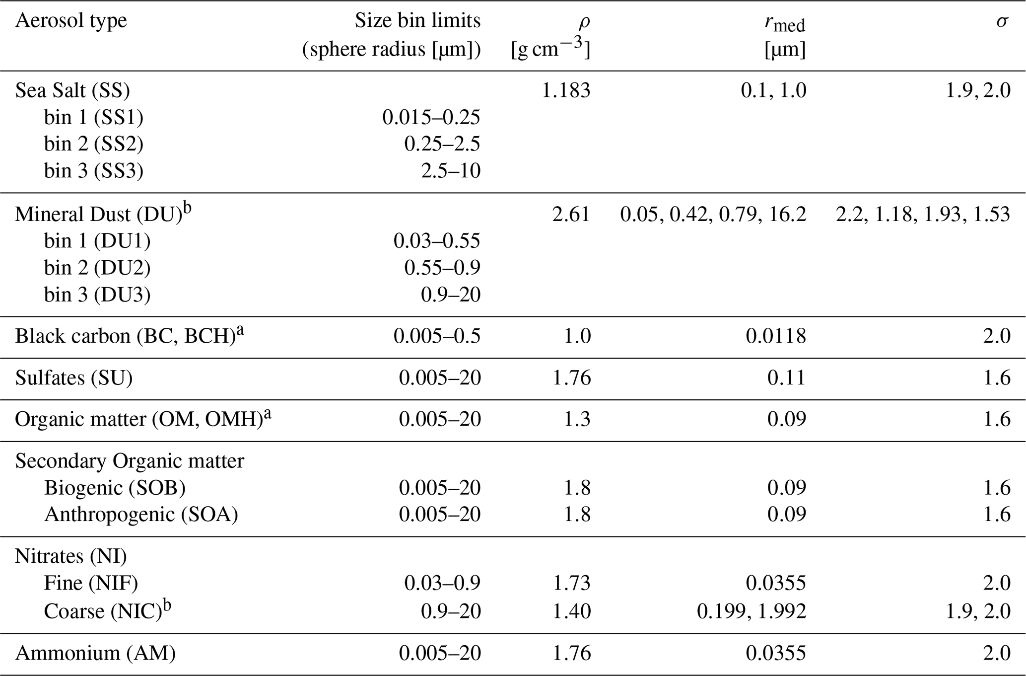
All species are hydrophilic, except those marked with ^a, which are represented by a hydrophilic and a hydrophobic tracer, and the letter H is used to indicate the hydrophilic tracer. Hydrophobic tracers and those marked with ^b are not used for CCN computations.

IFS-COMPO represents 8 types of aerosols in a bulk representation, which are reported in Table 1. Some species like sea salt (SS) consist of multiple partitions of a multimodal PSD, which is referred to as a “bulk-bin” representation. Bulk optical properties for each species are computed using Mie calculations with a prescribed log-normal number PSD, with median radius r_med and shape parameter (geometric standard deviation) σ (ECMWF, 2024a). Throughout this study, aerosol PSDs refer to dry aerosol, and the normalized distribution n(r) is defined as

$$\begin{array}{}\text{(1)}& n\left(r\right)=\sum _{i=\mathrm{1}}^N{a}_i{n}_i\left(r\right)=\sum _{i=\mathrm{1}}^N{\displaystyle \frac{a_i}{\sqrt{\mathrm{2}\mathit{\pi }}r\ln {\mathit{\sigma }}_i}}{e}^{-\frac{{\ln }^{\mathrm{2}}(r/r_{\mathrm{med},i})}{\mathrm{2}{\ln }^{\mathrm{2}}{\mathit{\sigma }}_i}}\end{array}$$

where i denotes a mode of the distribution and a_i are weighting coefficients such that $\sum a_i=\mathrm{1}$.

Hydrophilic species undergo hygroscopic growth by water uptake, described as a function of relative humidity, which affects refractive index and particle size through mixing with water, which are relevant for transport processes and radiative transfer calculations. Hydrophilic species undergo a removal process when precipitation occurs, with a fixed mass scavenging rate described in ECMWF (2024a) and following Luo et al. (2019).

The externally-mixed representation of CAMS aerosols has relevant consequences on process descriptions. For example, the optical properties of a mixed population are, by superposition assumption, given by the sum of its components. Moreover, the model is unable to represent those ageing processes where organic matter (OM), black carbon (BC) or sulfate (SU) particles cluster together to form new particles. While such ageing processes conserve the speciated aerosol mass, they naturally impact the total number, PSD and refractive index of the resulting aged species. To represent ageing, the IFS-COMPO converts OM and BC from the hydrophobic to the hydrophilic type with an e-folding timescale that can be either prescribed or depending on local chemical composition, but chemical and optical properties of the dry particles are unaffected. Hydrophilic OM undergoes hygroscopic growth, while hydrophilic BC is optically identical to the hydrophobic type, which represents pristine soot monomers. In reality, aged BC appears in the form of clusters or chain-like aggregates (e.g. Teng et al., 2019 and references therein) that agglomerate with SU, nitrate (NI) and ammonium (AM) crystals to form highly soluble, large structures. Observed OM also forms coatings around SU aerosol cores, eventually incorporating soot particles (Yu et al., 2019). While we cannot fully address the ageing issue in this study, more sophisticated representations of ageing processes might be a future area for improvement in CAMS, given the relevance of ageing for aerosol number concentrations and, ultimately, N_d.

Aerosol sources can depend on meteorological forcing (SS, DU, SU precursors), chemistry (secondary OM, NI, AM, SU), natural and anthropogenic emissions (SU, AM, NI, OM), including wildfires (OM, BC). While all species undergo sedimentation and dry deposition, wet scavenging by precipitation is the most efficient removal mechanism for hydrophilic aerosols in models. IFS-COMPO assigns each species a fixed wet scavenging coefficient indicating the mass fraction assumed to be dissolved in cloud water; this value is 0.7 for all hydrophilic species except SS (0.9) and AM (0.8) (ECMWF, 2024a). In mixed-phase conditions, a temperature-dependent modulation of the aerosol activated fraction from Verheggen et al. (2007) is applied when precipitating snow is produced.

Aerosol number concentrations can be obtained from mass concentrations with the number-to-mass ratio (J). For a given PSD of (spherical) particles, this is defined as

$$\begin{array}{}\text{(2)}& J={\displaystyle \frac{\mathrm{3}}{\mathrm{4}\mathit{\pi }\mathit{\rho }}}{\left(\underset{r_{min}}{\overset{r_{max}}{\int }}{r}^{\mathrm{3}}n\left(r\right)\mathrm{d}r\right)}^{-\mathrm{1}}\end{array}$$

where ρ is the aerosol density, and r_min and r_max are the aerosol bin boundaries.

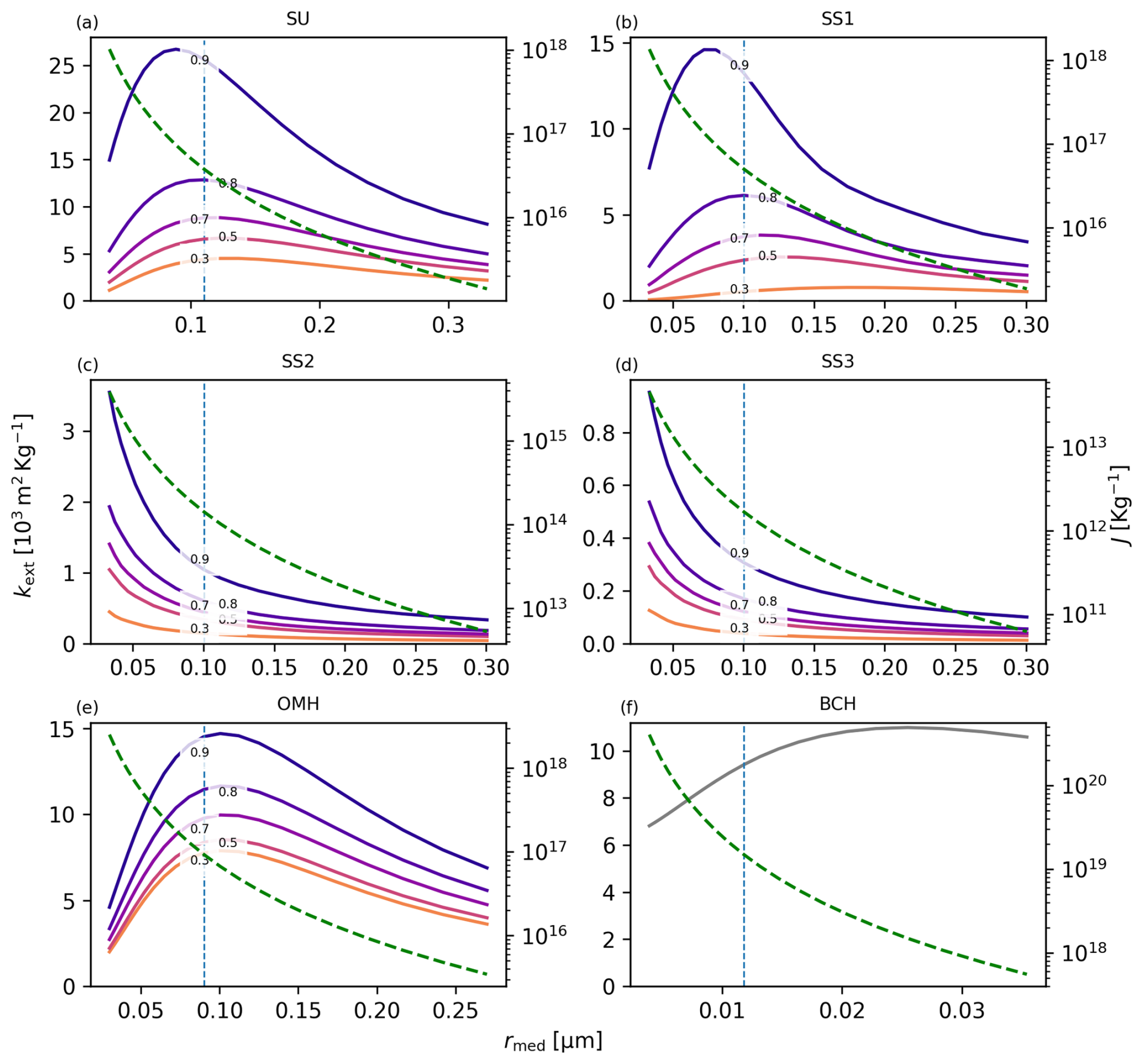
Figure 1 Mass extinction coefficient k_ext at 550 nm and number concentration per unit mass J (as defined in Eq. 2) as a function of the median radius r_med of the number PSD for the hydrophilic aerosol species listed in Table 1. Labels indicate selected relative humidity values. Nitrates and ammonium are not shown, but their optical properties are very close to sulfates for the purpose of this discussion. The dashed green line shows the number of particles per unit mass J as a function of r_med and its scale is given on the right of each plot. For each tracer, the vertical dashed line indicates the default dry median radius according to Table 1. For sea salt, the ratio between the median radii of the two modes $r_{\mathrm{med},\mathrm{2}}/r_{\mathrm{med},\mathrm{1}}$ was kept constant, and the dashed line indicates the location of the finer mode.

CAMS aerosols are routinely validated via observations of aerosol optical depth (AOD), particulate matter (PM) and surface concentrations of speciated aerosols. AOD is also operationally assimilated to produce CAMS analyses (Benedetti et al., 2009). However, most of these offer limited information about aerosol number concentrations. To illustrate this for AOD, Fig. 1 shows the dependency on r_med of J together with the 500 nm mass extinction coefficient (k_ext) for a selection of IFS aerosol tracers at different values of relative humidity. In most cases, curves are quite flat at the default value of r_med, indicating that k_ext is weakly dependent on small displacements of the PSD. This property characterises populations dominated by particles with radius r such that the ratio $x=\mathrm{2}\mathit{\pi }\mathit{\lambda }/r$ in the visible regime is close to the peak x≈6 of the Mie extinction efficiency (Petty, 2006). Consequently, relatively small changes of the aerosol PSDs have a potentially negligible impact on k_ext, but a large impact on J (1–2 orders of magnitude). The same also holds for small changes in the shape parameter σ (not shown). Nonetheless, AOD in the visible range (400 to 800 nm) is a weak constraint for aerosol particle number concentrations in a bulk representation. Therefore, we aim to make modest changes to aerosol PSD assumptions to optimise the prediction of N_d, while maintaining consistency with the AOD currently simulated by the system.

3 Observational datasets

The optimisation of aerosol PSD parameters presented in this work relies exclusively on MODIS N_d retrievals, while all other datasets (AERONET, CERES, VIIRS, MODIS AOD) are exclusively used for validation.

3.1 MODIS AOD

The MODerate Resolution Imaging Spectroradiometer (MODIS) is mounted on board the polar-orbiting Aqua and Terra satellites operated by NASA. For this study, we use monthly Collection 6.1 level 3 550 nm AOD observations covering the period 2003–2024 (Platnick et al., 2017a, b), produced with the Dark Target retrieval algorithm over land and sea (Levy et al., 2013; Sayer et al., 2014).

3.2 MODIS N_d

We also use daily MODIS N_d retrievals (Gryspeerdt et al., 2022a) produced by combining Level 2 MODIS 2.1 µm retrievals of cloud optical thickness τ and cloud-top effective radius (r_e) (Nakajima and King, 1990; Platnick et al., 2017c) under adiabatic (non-precipitating, non-mixing) cloud assumptions. N_d values are retrieved only for liquid-phase clouds with cloud-top temperature larger than 268 K (Gryspeerdt et al., 2022b). Several N_d datasets are included in Gryspeerdt et al. (2022a), each resulting from different sampling strategies aimed at targeting systematic error sources affecting satellite retrievals. The least restrictive sampling strategy follows Quaas et al. (2006) (Q06) and selects pixels with r_e>4 µm and τ>4. A second follows Grosvenor et al. (2018b) (G18) and also requires a pixel cloud fraction larger than 0.9 as well as minimal thresholds for satellite and solar zenith angles, to address errors associated with cloud measurements under slanted views (Maddux et al., 2010; Grosvenor et al., 2018b). A third follows Bennartz and Rausch (2017) (BR17) and, on top of all the above-mentioned filters, imposes a stacking order for r_e, that must increase with the wavelength of the deployed near-infrared channel (1.6, 2.2 or 3.6 µm) to discard non-adiabatic cloud profiles.

We use the Q06, G18 and BR17 N_d retrievals averaged to monthly means on the original 1°×1° rectangular grid for the period 2003–2020. We use Q06 as the optimisation target due to its broader spatio-temporal coverage, and define error bars as the full spread across the three datasets at each grid-point. This approach captures the sensitivity to known retrieval artifacts without assuming a specific error model.

3.3 VIIRS AOD and AE

The Visible Infrared Imaging Radiometer Suite (VIIRS) is mounted on board the Suomi National Polar-orbiting Partnership (SNPP) and NOAA-20 satellites, operated by NOAA. We use the Level 3 monthly 550 nm AOD and 550–865 nm Angstrom exponent (AE) products for the period 2023–2024, produced with the Deep Blue (Hsu et al., 2013) algorithm over land and the SOAR (Sayer et al., 2018) algorithm over the ocean.

3.4 AERONET AOD, AE and size spectra

The Aerosol Robotic Network (AERONET) is an extensive network of ground-based sun photometers, providing measurements of aerosol optical properties (Holben et al., 1998). We use daily cloud-cleared, quality-assured and fully calibrated (Level 2) 550 nm AOD and 440–870 nm AE observations, as well as daily cloud-cleared, quality-controlled (Level 1.5) aerosol PSD inversion products (Dubovik and King, 2000) for a selection of observational sites. We used all data between 2003 and 2024 available at each site.

3.5 CERES EBAF TOA broadband shortwave fluxes

The Clouds and the Earth's Radiant Energy System (CERES) instruments for the measurement of top-of-atmosphere (TOA) broadband shortwave (SW) and longwave (LW) radiation (Wielicki et al., 1996) are mounted on board the Aqua, Terra, SNPP and NOAA-20 satellites. For this study we use TOA broadband shortwave (SW) all-sky monthly fluxes from Edition 4.2 Energy-Balanced and Filled (EBAF) dataset (Doelling, 2022) for the period 2023–2024.

4 Method

This study on ACI considers only the first indirect aerosol radiative effect, excluding any direct impact on cloud lifetime. This choice focuses on the activation pathway, without the introduction of additional feedback mechanisms, and reflects the more limited understanding of the effect of aerosols on precipitation compared with first indirect and semi-direct radiative effects (Stier et al., 2024). Moreover, if lifetime effects were active, the optimisation problem would no longer be well-defined, as N_d changes would directly affect precipitation and cloud evolution, while the optimisation relies on stored cloud fields.

This section presents how we constrained aerosol number concentrations for the bulk IFS representation with satellite retrievals of droplet number concentrations (N_d). If N_i indicates the number concentration of the ith aerosol species in a set of p species and assuming that, for each species, all particles larger than a critical size activate into droplets, N_d can be written as

$$\begin{array}{}\text{(3)}& N_{\mathrm{d}}=\sum _{i=\mathrm{1}}^p{N}_{\mathrm{d},i}=\sum _{i=\mathrm{1}}^p{\mathit{\alpha }}_i{N}_i\end{array}$$

where N_d,i indicates the number of activated particles and α_i the activation rate for the ith species, as a general function of the local atmospheric composition, thermodynamics and dynamics. In terms of relative changes for a given species i:

$$\begin{array}{}\text{(4)}& {\displaystyle \frac{\mathrm{d}{N}_{\mathrm{d},i}}{N_{\mathrm{d},i}}}={\displaystyle \frac{\mathrm{d}{\mathit{\alpha }}_i}{{\mathit{\alpha }}_i}}+{\displaystyle \frac{\mathrm{d}{N}_i}{N_i}}\end{array}$$

Now we can estimate how a finite change in the median radius r_med can affect N_d. Let's consider as an example sulfate aerosol (frequently a dominant CCN provider) and a change in its PSD r_med from 0.10 to 0.08 µm. This will affect N_d by changing both the activation rate α_i and the particle number concentration N_i. The change in α_i derives from r_med determining the critical supersaturation (S_crit) distribution and thus the maximum supersaturation during ascent. Using results from Rothenberg and Wang (2016), we estimate $\left|\frac{\mathrm{\Delta }{\mathit{\alpha }}_i}{{\mathit{\alpha }}_i}\right|⪅\mathrm{0.2}$. Rothenberg and Wang (2016) report that r_med is also the strongest control on activation rates α_i, so that we can neglect from now on the potential effect of changing the geometric standard deviation σ and the hygroscopicity κ. The effect of the r_med change on the aerosol number concentration can then be estimated using Eq. (2) in the approximation of $r_{min}=\mathrm{0}$ and $r_{max}=\mathrm{\infty }$: $\mathrm{\Delta }{N}_i/N_i\approx \mathrm{\Delta }J/J\approx -\mathrm{3}\mathrm{\Delta }r/r$, so that $|\mathrm{\Delta }{N}_i/N_i|\approx \mathrm{0.6}$. Thus, the aerosol PSD median radius, r_med, exerts the strongest control on N_d through N_i, and secondarily through α_i. This ensures that, to a first order, we can estimate the impact of r_med on N_d by neglecting its impact on the S_crit curve, i.e. by avoiding new parcel ascent computations and keeping α_i constant. In addition to r_med, α_i is controlled by the updraft velocity w (Rothenberg and Wang, 2016), which is the only environment quantity that we will diagnose for estimating N_d.

On the basis of these premises, we implemented a simple and lightweight scheme to diagnose N_d that relies on a lookup-table (LUT) of pre-simulated parcel simulations. Such a scheme can be used either online when running the IFS or offline on stored data to infer N_d from local aerosol fields and environmental variables such as vertical velocity. Section 4.1 describes its design and interface with the IFS radiation scheme. Section 4.2 describes model data and processing used for the online N_d simulations and Sect. 4.3 describes the offline optimisation procedure.

4.1 The aerosol activation scheme

The activation process of a population of aerosol particles can be summarized in such a way that, depending on local aerosols, thermodynamics (S_sat) and kinetics (timescales of ascent and water vapor condensation), for each species all particles larger than a critical size activate into a droplet. Consequently, to describe N_d, a number PSD description is needed, while their mass PSD is required to compute the mass scavenged by precipitation. Depending on the aerosol species and cloud regime, it might be consistent to assume low variability for mass activated fractions (as done by the IFS-COMPO by assigning a prescribed value to each species) while still diagnosing a variable number activated fraction.

We used the adiabatic parcel ascent model by Rothenberg and Wang (2016) (Pyrcel) to simulate activation of heterogeneous aerosol particle populations. We stored the results of the offline simulations in a lookup table (LUT) that takes as input the parcel updraft velocity and the number concentration of a set of pre-defined CCN-providing aerosol species and returns number and mass activated fractions, as well as critical dry radii for each of them. Atmospheric variables are set to describe an air-parcel ascent with initial pressure 850 hPa, temperature 278 K and 98 % relative humidity, lifted for a minimum of 100 m until peak S_sat is reached.

Table 2 Definition of CCN-providing species. For each species the hygroscopicity κ as well as the median radius r_med and shape parameter σ of the log-normal distributions are listed. The column labelled with N reports the range of number concentrations considered; within this range, 7 geometrically spaced values are used for the Pyrcel simulations. Recipes are reported as mass mixtures of the IFS-COMPO species denoted by m_x, where x refers to species reported in Table 1. The scaling factors for each aerosol species are determined by the number-to-mass ratio J (see Eq. 2) associated with the CAMS default PSDs, such that the number contribution from each tracer is conserved when forming the mass mixtures.

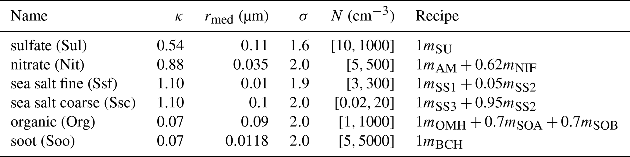
Previous studies found weak dependency of the activation process on cloud-base pressure and temperature, especially for warm phase regimes (above 273 K) (Leaitch et al., 1986; Rothenberg and Wang, 2016). We perform simulations for a range of vertical velocities w (updrafts) to also describe regimes with relatively high CCN concentrations (greater than 1000 cm⁻³, updraft-limited) (Pruppacher and Klett, 2010; Reutter et al., 2009; Rothenberg and Wang, 2016; West et al., 2014; Sullivan et al., 2016). To keep the number of simulations manageable, we define a small set of 6 internally-mixed CCN-providing aerosol species derived from those in Table 1, by grouping together those species with similar physico-chemical properties and assigning hygroscopicity κ with typical values inferred from Petters and Kreidenweis (2007). Their definitions are reported in Table 2. We performed activation simulations for every combination of number concentration for each species and vertical velocity (between 0.1 and 10 m s⁻¹) over seven geometrically-spaced values resulting in a total of 823 543 simulations. Subsequently, these results were integrated over Gaussian distributions of vertical velocities with seven values of mean $\stackrel{\mathrm{‾}}{w}$ in the range [−0.2 m s⁻¹, 0.2 m s⁻¹] (symmetric around zero, absolute values geometrically spaced) and seven geometrically-spaced values of standard deviation σ_w in the range [0.05 m s⁻¹, 2.5 m s⁻¹]. The integration is performed only for w>0 as in Golaz et al. (2011). The final size of the LUT is 5 764 801 elements.

The LUT returns activated number fraction (a_x) for each CCN-providing species x listed in Table 2 for a given mixture of particles and configuration of $\stackrel{\mathrm{‾}}{w}$ and σ_w. The activation scheme is in this sense a wrapper of the LUT accessor with pre- and post-processing capabilities that extracts the nearest-neighbor value along the aerosol concentrations dimensions, and linearly interpolates along the $\stackrel{\mathrm{‾}}{w}$ and σ_w dimensions. As a final step, the scheme computes the number of droplets N_d using Eq. (3) and returns it to the caller. The diagnosed N_d can be used online by the IFS radiation scheme to compute liquid droplets r_e (see below). Similarly, the LUT can be accessed offline to estimate N_d from a given aerosol population and updraft conditions. When running the IFS with prognostic aerosol tracers, the activation scheme can also be called a second time by the wet deposition code to diagnose the activated mass fraction for each hydrophilic species.

4.2 Activation scheme in the IFS (online)

The IFS (CY49R1) has a single-moment cloud microphysics scheme with prognostic variables for cloud fraction and water content for cloud liquid (LWC), cloud ice (IWC), rain (RWC) and snow hydrometeors. The radiation scheme diagnoses r_e needed for the all-sky radiative calculations:

$$\begin{array}{}\text{(5)}& r_{\mathrm{e}}={\left[{\displaystyle \frac{\mathrm{4}(\mathrm{RWC}+\mathrm{LWC})}{\mathrm{3}\mathit{\pi }{\mathit{\rho }}_{\mathrm{w}}\mathit{\gamma }{N}_{\mathrm{d}}}}\right]}^{\mathrm{1}/\mathrm{3}}\end{array}$$

where $\mathit{\gamma }={\left(\frac{r_{\mathrm{v}}}{r_{\mathrm{e}}}\right)}^{\mathrm{3}}$, with r_v mean volumetric ratio, ρ_w is the density of water and N_d the cloud droplet number concentration.

The IFS uses a wind-dependent parametrisation derived from Martin et al. (1994), such that, for 10 m winds between 0 and 10 m s⁻¹ $N_{\mathrm{d}}\in [\mathrm{40}{\mathrm{cm}}^{-\mathrm{3}},\mathrm{70}{\mathrm{cm}}^{-\mathrm{3}}]$ over the ocean and $N_{\mathrm{d}}\in [\mathrm{140}{\mathrm{cm}}^{-\mathrm{3}},\mathrm{170}{\mathrm{cm}}^{-\mathrm{3}}]$ over land. γ derives from the studies by Martin et al. (1994) and Wood (2000), and uses the values of 0.77 over ocean and 0.69 over land, with adjustments to represent increased dispersion of the cloud droplet PSD when drizzle is present. We redirect the reader to the IFS documentation (ECMWF, 2024b) for further details.

In the setup for this study, the IFS radiation scheme can diagnose N_d with a call to the activation scheme described above by providing as input $\stackrel{\mathrm{‾}}{w}$, σ_w and aerosol mass concentrations of all aerosol species required to construct the CCN providers of Table 2. $\stackrel{\mathrm{‾}}{w}$ is set equal to the large-scale vertical velocity, which is typical for climate models (Ghan et al., 2011; Van Noije et al., 2021). σ_w for turbulent boundary layers is generally diagnosed from turbulent kinetic energy (TKE) or eddy diffusivity (Ghan et al., 2011); however, these are not available as ERA5 fields, therefore for this study we used the Deardorff velocity scale w^∗ for convective boundary layers (Deardorff, 1970), scaled by a factor 0.6 to diagnose σ_w, in line with relationships found in observations and numerical simulations (Deardorff, 1970; Hogan et al., 2009). A minimum value of σ_w=0.1 m s⁻¹ is imposed to ensure physical activation conditions (e.g. Golaz et al., 2011; Barahona et al., 2014).

Autoconversion rates of cloud water to rain are computed using the parametrisation from Khairoutdinov and Kogan (2000) assuming fixed N_d values over land and sea, and this behaviour is left unchanged within this study, so that our setup does not include any direct impact of aerosols on cloud lifetime.

4.3 Activation scheme stored fields (offline)

To perform the offline N_d computations needed by the optimisation procedure we relied on stored aerosol fields originally produced for verification purposes from lower-resolution (triangular-linear TL255, ≈78 km) 1 d CAMS simulations initialised from ERA5 (Hersbach et al., 2020) over the period 2003–2020. Evaluations of the CAMS aerosol system (with and without assimilation of observations) can be found in Rémy et al. (2022) and in the CAMS validation reports released periodically (see e.g. Blake et al., 2025); near real-time validations are also publicly accessible using tools such as Aeroval (https://aeroval.met.no, last access: April 2026). Simulated aerosol fields were stored on 16 pressure levels between 10 and 1000 hPa; the 11 pressure levels below 100 hPa have thicknesses ranging between ≈640 and ≈2300 m, with the highest resolution found in the lower troposphere and lowest resolution in the mid-troposphere. Such a low vertical resolution is clearly suboptimal for the purpose of extracting accurate aerosol concentrations at cloud level; however, using these data enables us to assess the current state of the model and the potential of the optimisation procedure, which may partially compensate for resolution-driven inaccuracies.

4.4 Model data selection for the offline optimisation

We extracted from ERA5 the following fields for the period 2003–2020: pressure (p), temperature (T), cloud cover (f), liquid (LWC) and ice (IWC) water content. These cover the lowest 57 of the 137 IFS model levels, which correspond to up to 10 km altitude. For each data stream, we select within each month every fifth day starting on the third day of the month; for each day, we use 3-hourly data (00:00, 03:00, 06:00, …, 21:00 UTC). All fields are interpolated to the same 1°×1° grid of the N_d retrievals datasets.

For each column, only points with local time between 09:30 and 15:30 UTC are retained, to reflect the typical daytime overpasses of the Aqua and Terra satellites. Only cloudy model grid-boxes are then retained, defined as those with at least 10 % cloud fraction. For each column, we estimate the cloud optical thickness τ across all cloudy grid-boxes and retain only those columns for which τ>4 in line with Quaas et al. (2006).

We define the representative cloud-top level as the level at which the cumulative optical thickness from the top crosses the threshold of τ=2 and the cloud bottom where it reaches 95 % of the total cloud τ. Optical thickness is diagnosed offline assuming a constant extinction efficiency of Q_ext=2. We chose the cloud-top threshold for consistency with MODIS cloud-top properties being typically within τ≈1 in the infrared (Wang et al., 2014a), given that the extinction efficiency for wavelengths of ≈10 µm in liquid clouds is between 1 and 2 (Mitchell, 2000). Stratocumulus clouds also have optically thick and geometrically sharp cloud tops, spanning several units of optical thickness within one model level, which makes the results relatively insensitive to the precise choice of the optical thickness threshold for cloud-top identification. For completeness, we tested the sensitivity to cloud-top threshold values of τ=1 and τ=7, consistent with the bounds provided by correction formulas in Grosvenor et al. (2018a) for r_e retrievals. This affected cloud-top height location by less than 30 hPa for the thickest clouds and produced variations within 0.7 % in the global loss function (see below for its definition). Within a cloudy model column, we select liquid-phase clouds as those where at cloud top T>268 K, and $\mathrm{IWC}/(\mathrm{LWC}+\mathrm{IWC})<\mathrm{0.1}$ similarly to the observational filtering criteria, but allowing for some ice within the gridbox due to the coarse resolution of the model fields (1°×1°) compared to the Level-2 data from which the N_d datasets were derived (Gryspeerdt et al., 2022b).

For a cloud layer with constant N_d profile, the instantaneous finite relative change in τ obtained by a change in N_d, assuming all other variables unchanged (Twomey, 1991) is given by $N_{\mathrm{d}}^{\mathrm{1}/\mathrm{3}}$ scaling, while the relationship with $\mathrm{\Delta }{N}_{\mathrm{d}}/N_{\mathrm{d}}$ holds only for small perturbations:

$$\begin{array}{}\text{(6)}& {\displaystyle \frac{\mathrm{\Delta }\mathit{\tau }}{\mathit{\tau }}}={\displaystyle \frac{\mathrm{\Delta }{N}_{\mathrm{d}}^{\mathrm{1}/\mathrm{3}}}{N_{\mathrm{d}}^{\mathrm{1}/\mathrm{3}}}}={\displaystyle \frac{\mathrm{1}}{\mathrm{3}}}{\displaystyle \frac{\mathrm{\Delta }{N}_{\mathrm{d}}}{N_{\mathrm{d}}}}+\mathcal{O}{\left({\displaystyle \frac{\mathrm{\Delta }{N}_{\mathrm{d}}}{N_{\mathrm{d}}}}\right)}_{\mathrm{\Delta }{N}_{\mathrm{d}}/N_{\mathrm{d}}\to \mathrm{0}}^{\mathrm{2}}\end{array}$$

Throughout this study we set γ=0.8 consistently with the N_d retrieval methods by Gryspeerdt et al. (2022b). Despite the potentially regime-dependent impact of γ on cloud microphysics (Liu et al., 2006; Wang et al., 2023), there is currently no consensus on how this parameter should be represented in models. However, typical errors of assuming a fixed value for γ are estimated between 10 % and 14 % (see Grosvenor et al., 2018a and references therein), which translate into a relative error in τ of approximately 4 %, which we show below to be of secondary importance relative to that induced by aerosol number concentrations.

4.5 The offline optimisation procedure

At each stored time and for each column of the domain, we interpolate aerosols to the identified cloud-top level p and calculate aerosol number concentrations using Eq. (2). Given the relatively low vertical resolution of the aerosol dataset, the aerosol population extracted at cloud level represents a vertically smoothed average of actual simulated populations above and below the cloud level. The activation LUT is then used offline as a mapping function to diagnose N_d,IFS values from local aerosols and vertical velocity diagnostics. These are then averaged into monthly means, using only locations with at least three identified warm-phase cloud cases within the month. For each year, the simulated monthly-mean N_d are evaluated against the observed monthly-mean N_d,Q06 fields using the following loss function ℒ:

$$\begin{array}{}\text{(7)}& {\displaystyle }\mathcal{L}\left(N_{\mathrm{d},\mathrm{IFS}}\right)={∥{\displaystyle \frac{N_{\mathrm{d},\mathrm{IFS}}^{\mathrm{1}/\mathrm{3}}-N_{\mathrm{d},\mathrm{Q}\mathrm{06}}^{\mathrm{1}/\mathrm{3}}}{\mathrm{\Delta }{\stackrel{\mathrm{̃}}{N}}_{\mathrm{d},\mathrm{MODIS}}^{\mathrm{1}/\mathrm{3}}}}∥}_{\mathrm{2}}\text{(8)}& {\displaystyle }\mathrm{\Delta }{\stackrel{\mathrm{̃}}{N}}_{\mathrm{d},\mathrm{MODIS}}^{\mathrm{1}/\mathrm{3}}\equiv \underset{\mathrm{Q}\mathrm{06},\mathrm{G}\mathrm{18},\mathrm{BR}\mathrm{17}}{max}{N}_{\mathrm{d}}^{\mathrm{1}/\mathrm{3}}-\underset{\mathrm{Q}\mathrm{06},\mathrm{G}\mathrm{18},\mathrm{BR}\mathrm{17}}{min}{N}_{\mathrm{d}}^{\mathrm{1}/\mathrm{3}}\end{array}$$

where $\Vert \mathrm{\dots }{\Vert }_{\mathrm{2}}$ indicates the area-weighted average on the spherical surface and the source of N_d can be the offline diagnostics (IFS) or one of the three MODIS sampling strategies: Q06, G18, BR17 (Gryspeerdt et al., 2022b). Among the retrievals, N_d,Q06 was chosen as the optimisation target since Q06 is the least restrictive sampling strategy, which implies the largest number of valid retrievals.

As an optimisation algorithm for the loss function ℒ we use Nelder-Mead with free bounds, a popular minimisation method belonging to the class of direct search methods, i.e. that do not require knowledge of the gradients of the function, for functions of the kind f(ℝⁿ)→ℝ, which is the case for the constructed ℒ. The algorithm uses n-dimensional simplexes and performs a series of reflection, expansion and contraction operations to converge on function minima (see e.g. Lagarias et al., 1998). Across the many setups considered, we never encountered important convergence issues.

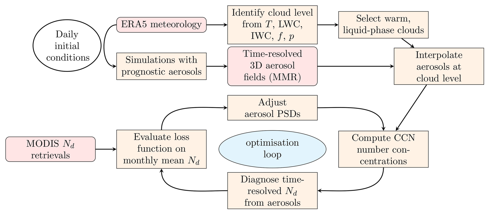
Figure 2 Flowchart of the optimisation procedure used to adjust aerosol particle size distributions (PSDs). This is performed over a time window of 1 year for each of the 18 years of the study.

The optimisation procedure is illustrated in the flowchart of Fig. 2. For each year from 2003 to 2020, ℒ is evaluated on monthly N_d using aerosol number concentrations from Eq. (2). The procedure is repeated in a loop leaving the median radius r_med as a free parameter for each CCN species excluding the coarse sea salt mode (Ssc), for which the median radius is fixed to 10 r_med,ssf.

While aerosol and cloud data are spatially co-located, only monthly mean values are compared, so that ℒ can be seen as a statistical evaluation of the simulated N_d. This implies that the optimisation targets large-scale and seasonal N_d signals, with variability on monthly and longer timescales. As a result, the sensitivity to the co-location in time and space of cloud fields and satellite overpasses is reduced. At the same time, by considering a smaller number of samples within each month we can substantially reduce the volume of data processed, keeping the procedure manageable.

As a result, a collection of optimised median radii for each species x and year y is obtained, $r_{\mathrm{med},x,y}$. We finally define the optimal PSD as those using the effective median radius $\stackrel{\mathrm{‾}}{r_{\mathrm{med},x}}\equiv {\mathrm{med}}_y\left(r_{\mathrm{med},x,y}\right)$, i.e. the median across the 18 years of the optimised median radii. Within this framework, the resulting optimised aerosol PSDs are constrained by the cloud-top N_d observations and represent an effective description of aerosol number consistent with these observations; their realism is conditioned by non-represented processes (e.g. diagnostic representation of N_d and absence of prognostic droplet microphysics) and aerosol biases (e.g. speciation and vertical structure), and is therefore evaluated a posteriori through independent observations of aerosol optical properties.

5 Results of the N_d optimisation

This section reports the outcome of the optimisation for three setups: a first one diagnosing N_d from aerosols found at the cloud-top level (InCloud, Sect. 5.1), a second one excluding BC from the CCN species (InCloudNoBC, Sect. 5.2), and a third one using aerosols found three levels below the cloud base (ClBase3, Sect. 5.3). Although CCN activation mainly occurs at cloud base, the model does not represent aerosol as explicitly dissolved within cloud droplets. The aerosol at cloud top has nevertheless been transported there by the same turbulent mixing and advection processes that transport cloud water. In that sense, the aerosol population co-located with cloud droplets at cloud top (InCloud) provides a possible first-order diagnostic representation of the aerosol environment at cloud-top N_d, although activation occurs at cloud base. The InCloudNoBC and ClBase3 setups are presented to check the robustness of the procedure to the CAMS BC representation and to the aerosol vertical profiles. Finally, we report in Sect. 5.4 the results of offline aerosol optics (speciated AOD and AE) simulations using the prior (CAMS default) and optimised (InCloud) effective PSD parameters.

5.1 N_d from cloud-top aerosol (InCloud)

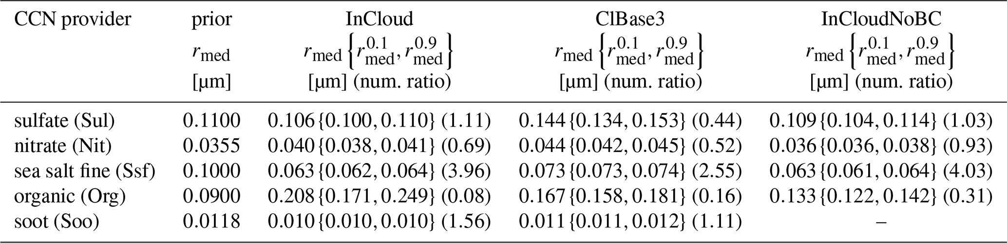
The optimal median radii and implied number scaling for all three optimisation setups are reported in Table 4, while Fig. 3 shows how the simulated N_d compares with the optimisation target (N_d,Q06) before (prior, CAMS default PSDs) and after optimisation (optimised), for the InCloud and ClBase3 setups. These are represented as relative differences in $N_{\mathrm{d}}^{\mathrm{1}/\mathrm{3}}$, defined as

$$\begin{array}{}\text{(9)}& \mathrm{RDND}={\displaystyle \frac{\mathrm{\Delta }{N}_{\mathrm{d}}^{\mathrm{1}/\mathrm{3}}}{N_{\mathrm{d},\mathrm{Q}\mathrm{06}}^{\mathrm{1}/\mathrm{3}}}}={\displaystyle \frac{N_{\mathrm{d},\mathrm{IFS}}^{\mathrm{1}/\mathrm{3}}-N_{\mathrm{d},\mathrm{Q}\mathrm{06}}^{\mathrm{1}/\mathrm{3}}}{N_{\mathrm{d},\mathrm{Q}\mathrm{06}}^{\mathrm{1}/\mathrm{3}}}}\end{array}$$

which serves as a proxy quantity for expected first-order relative changes in τ (see Eq. 6). The absolute zonal-temporal $N_{\mathrm{d}}^{\mathrm{1}/\mathrm{3}}$ RMSE is also shown in Fig. 3.

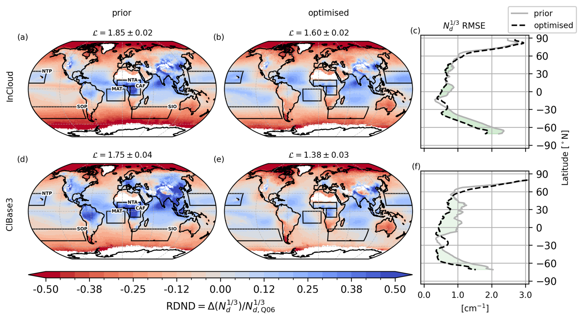
Figure 3 Offline-simulated mean N_d for the 18-year optimisation period from prior (IFS-COMPO default) (a, d) and optimised (b, e) aerosol PSDs, shown as relative differences in $N_{\mathrm{d}}^{\mathrm{1}/\mathrm{3}}$ (RDND) maps (a, b, d, e) and zonal $N_{\mathrm{d}}^{\mathrm{1}/\mathrm{3}}$ RMSE (c, f) with respect to the MODIS N_d optimisation target, Q06. These are for the optimisation setups InCloud (aerosols diagnosed at cloud level – panels a–c) and ClBase3 (aerosols diagnosed three model levels below cloud base – panels d–f). Negative RDND values indicate that MODIS N_d (Q06) values exceed the simulated values. Labelled boxes indicate regions used for regional evaluation and are presented later in Table 3 and Fig. 4. For each map, the corresponding loss function ℒ value (see Eq. 7) is reported.

The optimal PSDs resulting from the InCloud setup imply reduced number per unit mass J for nitrate (Nit, ×0.69) and organics (Org, ×0.08) CCN species but an increased value for sulfate (Sul, ×1.11) and fine sea salt (Ssf, ×3.96) (see Table 4). Figure 3 shows that the optimal PSDs globally improve the simulated N_d, corresponding to a reduction of the prior evaluation of the loss function ℒ (Eq. 7) by 13 %, from 1.85±0.02 to 1.60±0.02. The strongest reductions in absolute $N_{\mathrm{d}}^{\mathrm{1}/\mathrm{3}}$ (−0.25 to −0.5 cm⁻¹) are at the equator, where the prior N_d have a strong positive bias associated with OM-dominated CCN over Central Africa (RDND⪆0.50), and at latitudes south of 30° S, where model N_d are negatively biased ($\mathrm{RDND}⪅-\mathrm{0.50}$). However, moderate (RDND up to ≈0.2) residual bias patterns persist throughout the tropics and at latitudes south of 45° S, as shown by Fig. 3. Subtropical open-sea regions are also visibly degraded after the optimisation (RDND from ≈0.05 to ≈0.15). The low N_d bias over Australia worsens after optimisation (RDND from $\approx -\mathrm{0.15}$ to $\approx -\mathrm{0.3}$) as a result of the reduction of J for Org species.

We selected eight regions to better investigate remaining biases after the optimisation procedure: north tropical Africa (NTA), mid-Atlantic (MAT), central Africa (CAF), north tropical Pacific (NTP), Southern Indian Ocean (SIO), Southern Pacific (SOP), Europe (EUR) and India (IND). Their extents are reported in Table 3 and illustrated in Fig. 4. Figure 3 shows that the NTA, MAT, CAF, NTP regions all suffer from a high N_d residual bias relative to N_d,Q06 after the InCloud optimisation (RDND between ≈0.15 and ≈0.30), while SIO and SOP regions are biased low ($-\mathrm{0.15}⪆\mathrm{RDND}⪆\mathrm{0}$). For these two groups of regions, monthly observed and simulated N_d are illustrated as spider plots in Fig. 5. In the NTP region, both prior and optimised model N_d are within the uncertainty range of the observations, while for the SIO and SOP regions, despite a significant increase in simulated N_d after optimisation, these remain below the lower end of the uncertainty range, typically found at ≈60 cm⁻³. Finally, in the NTA, MAT and CAF regions, the prior simulated N_d exceeds the upper bound of the uncertainty range with a clear seasonal pattern: December–February for NTA, December–March and June–September for CAF, July–October for MAT. After optimisation, N_d values fall within the uncertainty range in all three regions, but tend to remain near the upper bound and biased high with respect to N_d,Q06 (Fig. 5) during these periods. Aerosol speciation in these three regions indicates that 60 %–90 % of simulated N_d originates from OM and BC particles (not shown), which are typically associated with wildfires.

Table 3 Domain definitions for regional N_d evaluation.

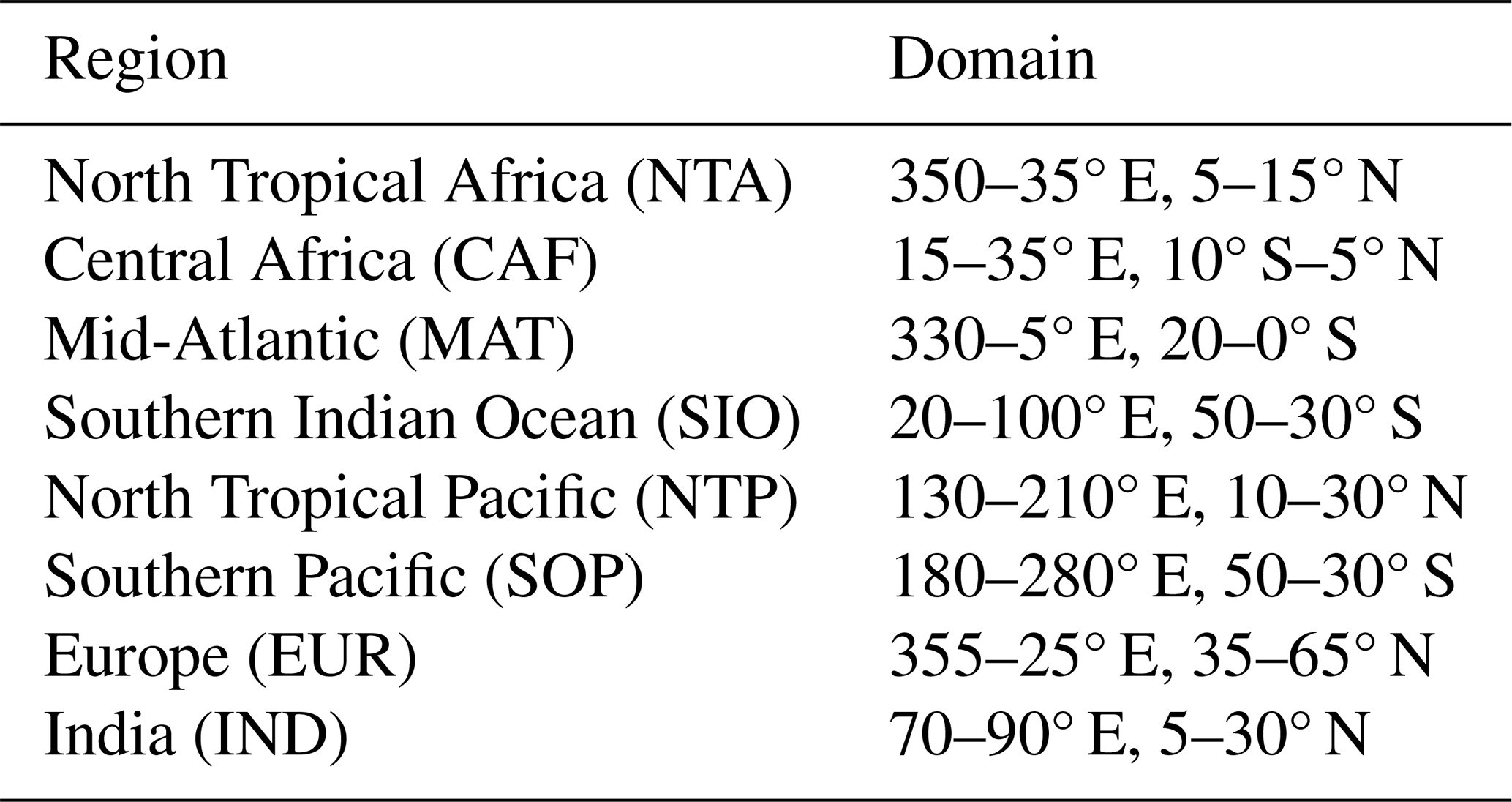
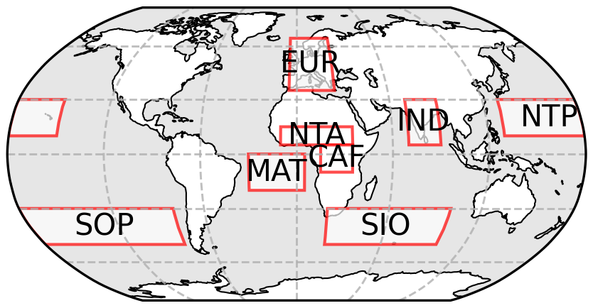
Figure 4 Map of regions defined in Table 3.

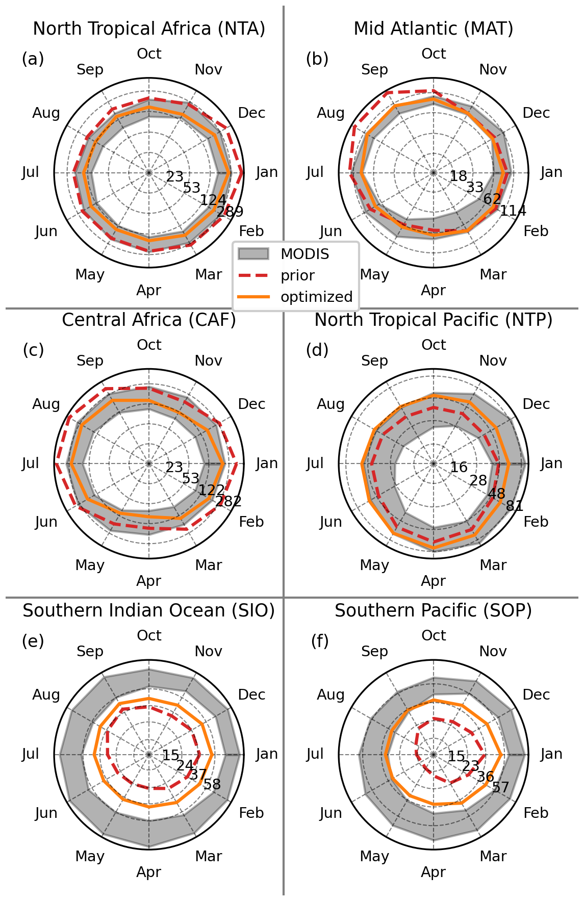
Figure 5 Simulated and observed monthly N_d (in units of cm⁻³) for the NTA, NTP, CAF, SOP, MAT, SIO regions (see Table 3 and Fig. 4) over the 2003–2020 period. Simulated values correspond to the CAMS default PSDs (prior) and the effective PSD parameters resulting from the InCloud optimisation setup (optimised). Shaded areas indicate the range of mean values spanned by the MODIS N_d retrieval datasets (see Eq. 8). Note that the N_d scale is nonlinear.

5.2 N_d without black carbon (InCloudNoBC)

If BC is excluded from the CCN calculations, the resulting optimal aerosol PSDs produce effects qualitatively consistent with InCloud, but with a significantly weaker reduction for Nit (×0.93) and Org (×0.31) CCN species (Table 4). For this setup, optimal PSDs for all species except fine sea salt (Ssf) are closer to the prior PSDs than for InCloud (Table 4). At the end of the InCloudNoBC optimisation, $\mathcal{L}=\mathrm{1.62}\pm \mathrm{0.03}$, so that the final result is not significantly different from that of InCloud ($\mathcal{L}=\mathrm{1.60}\pm \mathrm{0.02}$). Similarly, we found no significant difference in RDND between the optimised InCloudNoBC and InCloud N_d (not shown).

Table 4 Optimisation results summary for each CCN-providing species (see Table 2) and each of the three optimisation setups described in the text. Reported are prior and optimised PSD median radii r_med, 0.1 and 0.9 quantiles $r_{\mathrm{med}}^{\mathrm{0.1}}$ and $r_{\mathrm{med}}^{\mathrm{0.9}}$ and the implied number ratio $J_{\mathrm{optimised}}/J_{\mathrm{prior}}$. For sea salt coarse (Ssc), $r_{\mathrm{med},\mathrm{ssc}}=\mathrm{10}{r}_{\mathrm{med},\mathrm{Ssf}}$, therefore the number ratio is identical to Ssf.

5.3 N_d from below cloud-base aerosol (ClBase3)

If N_d is diagnosed using aerosols located three model levels below cloud base, optimal PSDs imply a strongly reduced J for Sul (×0.44), Nit (×0.52) and Org (×0.16), and a higher J for Ssf (×2.55) (see Table 4). For all species except Ssf, the optimal r_med values are significantly larger than for the InCloud setup. For the optimised ClBase3 setup, $\mathcal{L}=\mathrm{1.38}\pm \mathrm{0.03}$; this setup is markedly better than InCloud at matching MODIS N_d due to the lower $N_{\mathrm{d}}^{\mathrm{1}/\mathrm{3}}$ RMSE (Fig. 3) at latitudes south of 30° S over the ocean, where $\left|\mathrm{RDND}\right|⪅\mathrm{0.15}$.

5.4 Consistency of optimal PSDs with aerosol optics

Figure 6 shows that the optimised (InCloud) PSDs for the group of aerosols including SS and NI tend to slightly increase AOD, with a larger relative impact at mid- to high latitudes in the Southern hemisphere, while the low-latitude signal is dominated by the reduced AOD from the group of OM, SOA, SOB aerosols. Overall, the mean and local impact (not shown) on total visible AOD remains typically within a 15 %, partly also due to a compensation between the two aerosol groups. The increase in SS AOD at latitudes south of 30° S provides the largest relative change in total AOD, which improves the DJF season and degrades the JJA season.

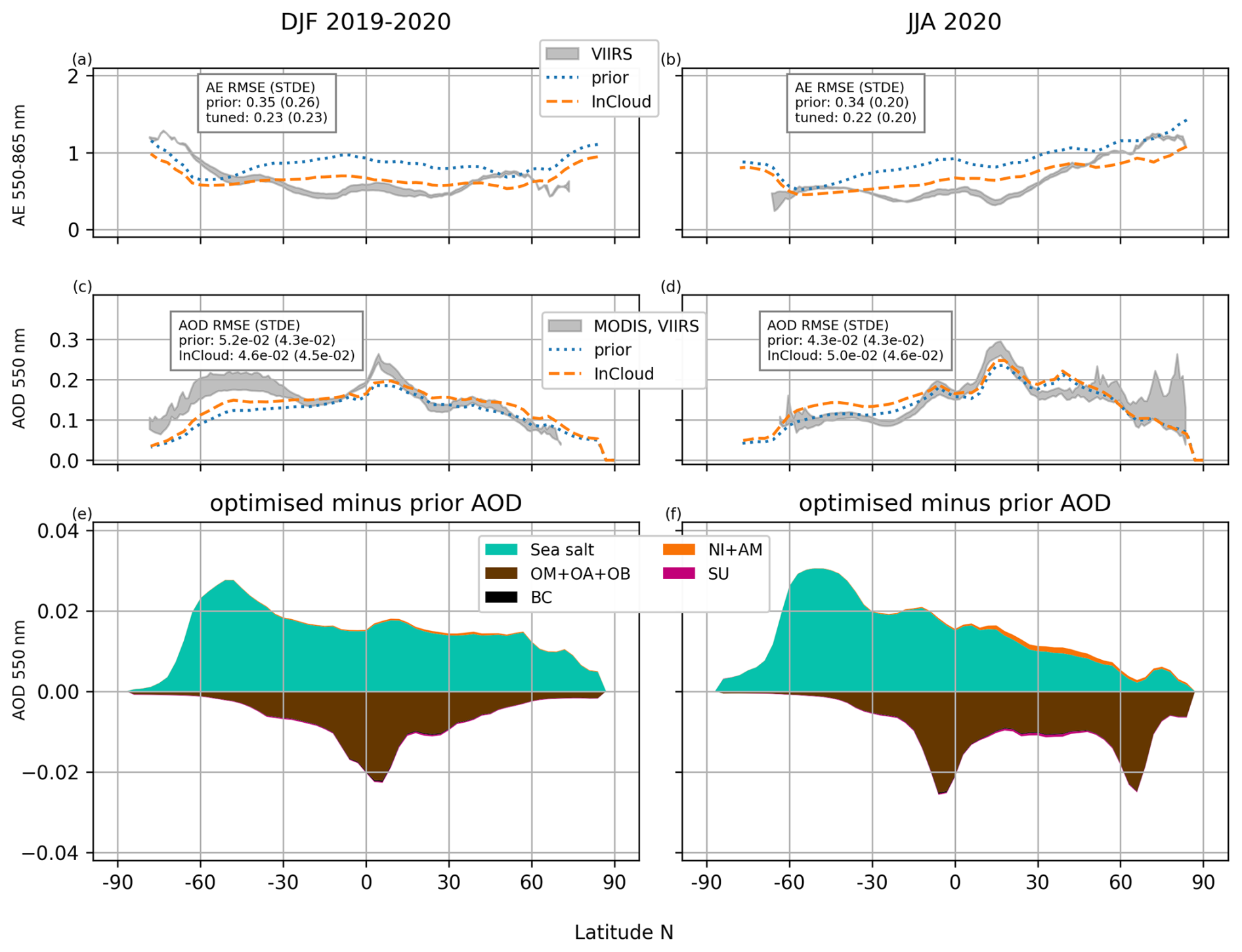
Figure 6 Simulated aerosol optical properties over the ocean for the DJF 2019–2020 (a, c, e) and JJA 2020 (b, d, f) seasons from Mie computations using the prior IFS aerosol definitions from Table 1 (prior), and using the median radii obtained from the InCloud N_d optimisation setup from Table 4 (InCloud). Panels (a) and (b) show the zonal mean Angstrom exponent (AE) (550–865 nm), panels (c) and (d) show the zonal mean 550 nm AOD. Global RMSE in space for the seasonal mean values of simulated AE and AOD is also reported. The grey shading indicates the range of observed zonal mean values from VIIRS (NOAA20 and SNPP) for the AE and, for AOD, including also MODIS (Aqua and Terra). The bottom panels (e, f) show the optimised-minus-prior AOD difference as a broken down by aerosol species.

The change in AE due to the optimised (InCloud) PSDs is dominated (> 90 %) by the SS2 and SS3 aerosol (not shown). This is detrimental at the latitudes higher than 45° in the Summer hemisphere, where the model tends to be biased low, but mostly beneficial everywhere else. As a result, the global AE RMSE is reduced by more than 34 % for both seasons, as shown by Fig. 6.

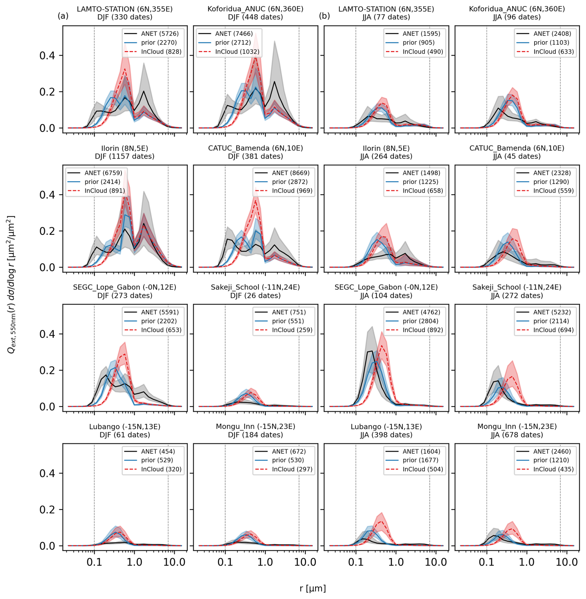
Figure 7 Aerosol size spectra (see Eq. 10) for several low-latitude AERONET sites during the DJF (a) and JJA (b) seasons. The distribution is represented in terms of the spherical geometric cross-section (σ, see Eq. 10) weighted by the Mie extinction efficiency at 550 nm for a real refractive index 1.3. Sites are ordered from top to bottom by decreasing latitude. AERONET spectra (ANET) are derived from all available observation dates, with total number of dates reported after the season label, and the corresponding IFS spectra were computed offline from experimental outputs for the seasons DJF2023–24 and JJA 2024, using both the prior and InCloud (optimised) PSD definitions (see Table 4). After each label, the total column particle number concentration is reported, calculated over the domain [0.1 µm, 0.7 µm], with unit 10⁻³ µm⁻² (indicated by the dashed vertical lines), interpretable as the mean number concentration expressed in cm⁻³ for a 1 km-deep layer with the same total-column amount of particles.

Figure 7 shows aerosol size spectra as observed by AERONET and simulated from CAMS aerosols for sites located close to the NTA and CAF regions. The plotted quantity is the PSD of the total spherical geometrical cross-section:

$$\begin{array}{}\text{(10)}& {\displaystyle \frac{\mathrm{d}\mathit{\sigma }}{\mathrm{d}\ln r}}=\mathit{\pi }{r}^{\mathrm{2}}r{\displaystyle \frac{\mathrm{d}N}{\mathrm{d}r}}\end{array}$$

weighted by the Mie extinction efficiency Q_ext(r) at 550 nm for a real refractive index 1.3. Stations north and south of the equator present a peak in AOD during the DJF and JJA seasons, respectively, which is consistent with regional wildfire seasons. Multimodal size spectra are found for the stations north of the equator, with peaks at ≈0.1 µm, ≈0.6 µm and ≈2 µm. The two coarser peaks are also present in simulated spectra and are produced by mineral dust likely advected by northerly trade winds from West Africa. The finest-mode peak produced by the model is found at ≈0.3 µm (associated with OM aerosol), while it is located at less than 0.2 µm or even 0.1 µm in the AERONET data. Despite the particle number being generally underestimated by the model, the overall area below the graph in the r<1 µm regime is in fairly good agreement between model (prior) and observations. Using the optimised (InCloud) PSD definitions (see Table 4) produces a modest shift in the size spectra of the finest peak, which is associated with OM aerosol, toward larger values, resulting in visibly degraded size spectra and deepening the low aerosol number bias against AERONET.

6 Testing changes in the aerosol wet-scavenging scheme

The results presented in Sect. 5 reveal a pattern of low N_d biases at mid- to high latitudes (above 60° N and 45° S), that persist at the end of the optimisation. In these regions, aerosol concentrations tend to decrease sharply in the in-cloud relative to the below-cloud environment, typically coincide with precipitating mixed-phase clouds. This motivated targeted sensitivity experiments to investigate the contribution of aerosol wet removal in regulating simulated CCN availability.

We initially collected diagnostics of in-cloud (rain-out, IN-SCAV) and below-cloud (wash-out, BC-SCAV) wet scavenging as well as the release by precipitation evaporation (EVAP). These confirm the expectation that IN-SCAV from large-scale precipitation dominates the removal of SU and SS, while EVAP is significant in modulating tropical and subtropical aerosol mass budgets. For latitudes larger than 55° and along the intertropical convergence zone (ITCZ) we found residence times due to IN-SCAV below 1 d for the entire column of SS (10 h) and SU (18 h).

We focused on the representation of the IN-SCAV parametrisation for precipitating mixed-phase (MP) clouds, characterised by temperatures between −38 and 0 °C and coexistence of supercooled liquid water and ice. Under these conditions, the IFS IN-SCAV scheme diagnoses aerosol removal rates by separately relating snow and rain formation respectively to ice and liquid cloud condensate. Aerosol scavenged mass fraction from snow is then modulated by a factor $\mathit{\zeta }\in [\mathrm{0},\mathrm{1}]$, which is provided by the temperature-dependent parametrisation from Verheggen et al. (2007), denoted here as ζ(T). Based on the same observational dataset, Verheggen et al. (2007) also proposed an alternative parametrisation as a function of the cloud ice water ratio $\mathrm{IWR}=\mathrm{IWC}/(\mathrm{IWC}+\mathrm{LWC})$, ζ(IWR), that has since been deployed in several aerosol modelling studies (e.g. Hoose et al., 2008; Liu and Matsui, 2021).

We present here results from two modified IN-SCAV formulations:

• MOD1 uses ζ(IWR) to scale activated mass fraction both when either snow or rain is produced in mixed-phase conditions, rather than using ζ(T) only for snow;

• MOD2 adds the following to the setup of MOD1:

  • diagnose the aerosol removal rate using the ratio between the precipitation formation and the total cloud condensate instead of treating the ice and liquid phases separately;

  • ζ=1 at regimes where riming prevails, identified with T between 261 and 265 K when LWC>1 g m⁻³ following Qi et al. (2017).

6.1 Online IFS-COMPO experiments

To test the sensitivity of ACI to aerosol wet removal in mixed-phase clouds, we performed a series of online IFS-COMPO simulations. These use meteorological initial conditions from ERA5 analyses, while chemical and aerosol tracers are restored from the previous forecast day at valid time +24 h, thus leaving them free to evolve. These runs have a resolution of ≈39 km.

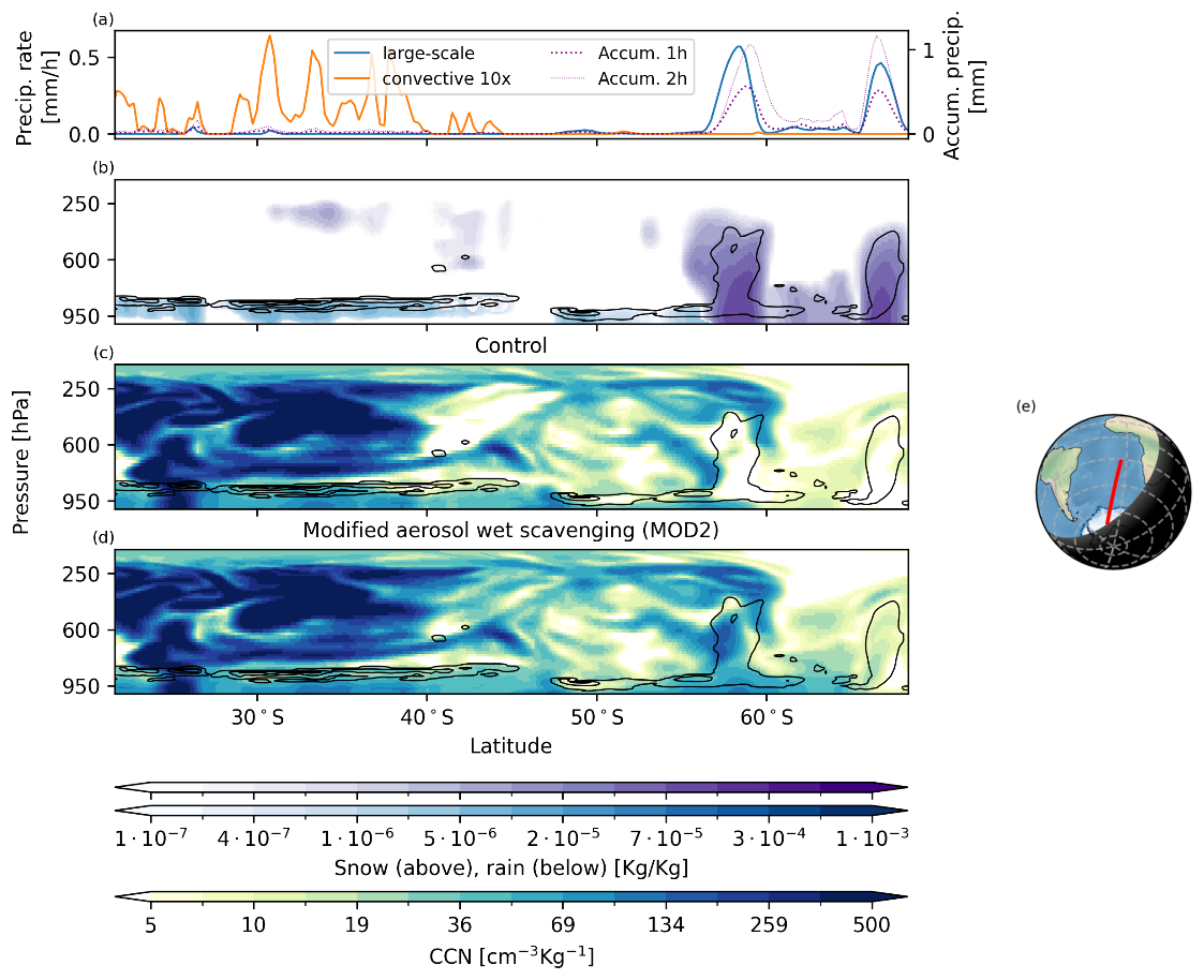
Figure 8 Cross-section of IFS-COMPO simulation (online) on 18 September 2024, 15:43 UTC. From top to bottom, total instantaneous large-scale and convective precipitation rates, and accumulated total precipitation (1, 2 h) at the surface (a, note that instantaneous convective precipitation is multiplied by a factor 10 for visualisation). Panel (b) shows the cross-section of instantaneous specific rain and snow water contents; panel (c) shows the cross-section of CCN_max, defined as the sum of the number concentrations from Sulfate (SU), Sea Salt bin 1 (SS1) and Organic Matter (OM) aerosol; (d) as in panel (c) but for the MOD2 simulations. Black contours in panels (b)–(d) indicate total cloud specific water content (first contour at $\mathrm{2}\times {\mathrm{10}}^{-\mathrm{5}}$ and spacing by $\mathrm{5}\times {\mathrm{10}}^{-\mathrm{5}}$). The track location on the globe is shown in panel (e).

Figure 8 displays a cross-section of the simulation output for a case study on 18 September 2024, after a 10 d spin-up. We use aerosol number mixing ratios (computed from prior CAMS PSDs), i.e. aerosol number concentration per unit mass of air, for Sulfate (SU), Sea Salt bin 1 (SS1) and Organic matter (OM) as an upper-bounding proxy (CCN_max) for CCN concentrations. This case shows that for the control simulation CCN_max drops to extremely low values (well below 10 cm⁻³) in mixed-phase clouds simulated over the Southern Ocean. With the MOD2 version of the model, CCN_max is significantly higher throughout the same ice-containing cloud profiles, with values up to 100 cm⁻³. CCN_max is also increased at lower latitudes, where snow is present aloft, which is particularly evident at 42° S, between 650 and 250 hPa.

We also tested MOD1 and MOD2 by performing more extended simulations over the boreal winter (DJF) 2023–2024 and boreal summer (JJA) 2024 seasons. These setups use a 1-month spin-up to ensure that tracers are aligned with the climate of the model. For these cases, the “Control” experiment uses the default IFS CY49R1, where N_d do not depend on aerosols, “InCloud” diagnoses N_d from aerosols (ACI) at cloud level using the InCloud optimal PSDs, while MOD1 and MOD2 experiments add the corresponding IN-SCAV modifications on top.

6.2 TOA SW flux diagnostics

Figure 9 shows the top-of-atmosphere (TOA) biases in simulated SW fluxes against CERES for the DJF 2023–2024 season experiments. The InCloud (ACI) experiment exhibits both larger absolute bias (+3.5 W m⁻²) and error standard deviation (STDE, +2.1 W m⁻²) than Control. The strongest contribution to this degradation is over the Southern Ocean, where TOA SW biases are increased by ≈20 W m⁻² in the sense of reduced cloud albedo. With the InCloud-MOD1 and InCloud-MOD2 experiments, STDE is reduced respectively by 1.1 and 1.7 W m⁻² compared to InCloud, with reflected SW radiation over the Southern Ocean increasing by up to ≈20 W m⁻².

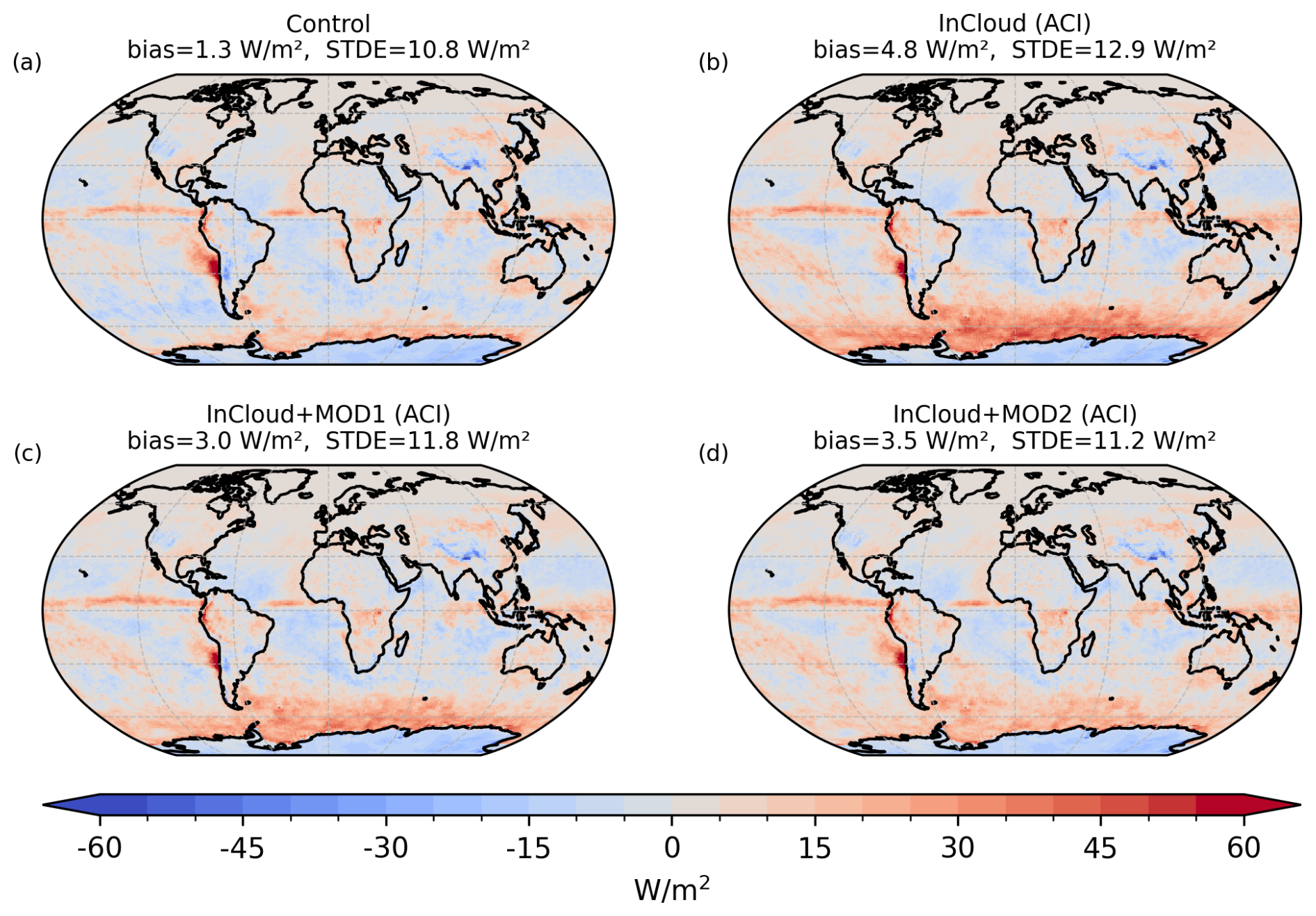
Figure 9 Mean top-of-atmosphere (TOA) shortwave (SW) radiation flux (outgoing), CERES minus IFS difference for the season DJF 2023–2024, with global bias and error standard deviation (STDE) on monthly means for each experiment. For the control simulation (a) N_d does not depend on aerosols; in panels (b)–(d) N_d is diagnosed from aerosols (label ACI) using optimal PSDs from the InCloud setup. These use the default IFS IN-SCAV configuration (b), MOD1 (c) and MOD2 (d). Details are provided in the text.

6.3 AOD, AE and aerosol size spectra

We evaluate mean model outputs using mean observations of all available AERONET 550 nm AOD, 440–870 nm AE and size spectra over the period 2004-2024 at several high-latitude stations, six in each hemisphere. These are shown in Fig. 10 and cover the summer season (DJF for the southern and JJA for the northern hemisphere).

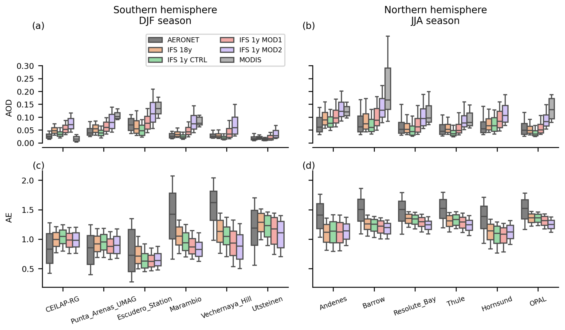
Figure 10 Boxplots of AOD (a, b) and Angstrom exponent (AE) (c, d) for high-latitude AERONET sites in the southern (a, c) and northern (b, d) hemisphere, as in Fig. 11. Box edges mark the interquartile range, and the whiskers indicate the 0.1 and 0.9 quantiles. The AERONET and MODIS (Aqua and Terra means) data cover the period 2003–2020. MODIS values are shown in panels (a) and (b) only where at least 10 months of valid retrievals are available. AERONET means are based on a limited number of valid daily observations, typically between 200–800 d per site, with substantially fewer observations for the Escudero site (47 d). The simulated values labelled “IFS 1y” refer to the 1-year simulation for the Control (CTRL), MOD1 and MOD2 setups. To facilitate comparison across the different periods of observational and simulation coverage, simulated values based on the stored aerosol fields used for the optimisation, covering 2003–2020 (“IFS 18y”), are also shown.

Figure 10 shows AOD and AE boxplots for the selected AERONET stations. The control simulation produces comparable 550 nm AOD with respect to AERONET, but tends to be biased low relative to the colocated MODIS AOD for most sites with enough valid retrievals. The model also tends to produce systematically low AE (up to $\approx -\mathrm{0.8}$) against AERONET, but this difference is only occasionally larger than the joint model-observations interquartile range. The MOD1 and MOD2 simulations result in generally increased AOD (up to +0.05) and decreased AE (up to −0.5) for all locations, which represent a degradation with respect to mean AERONET observations.

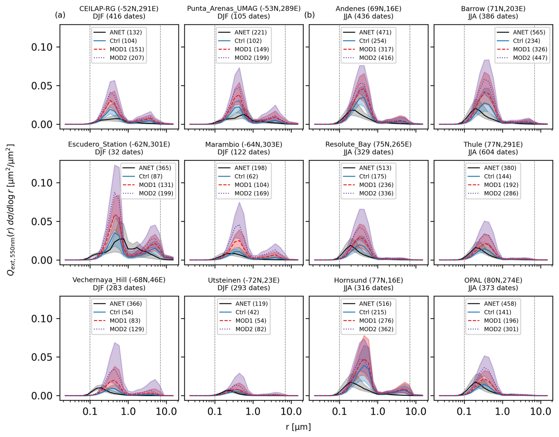
Figure 11 Aerosol size spectra at a selection of high-latitude AERONET locations, respectively for the southern (a, season DJF) and northern (b, season JJA) hemisphere. Like in Fig. 7, spectra are represented using the spherical geometric cross-section (σ) weighted by the Mie extinction efficiency at 550 nm for a real refractive index 1.3. Sites are ordered from top to bottom by increasing (absolute) latitude. AERONET spectra (ANET) are from all available observation dates (total number after the season label), while the corresponding IFS spectra are calculated offline from experimental outputs for the seasons DJF2023-24 and JJA 2024 using the two changed mixed-phase clouds wet scavenging parametrisations MOD1 and MOD2. After each label are reported total column particle number concentrations calculated over the domain [0.1 µm, 7 µm] (indicated by the dashed vertical lines), with unit 10⁻³ µm⁻², interpretable as the mean number concentration expressed in cm⁻³ for a 1 km-deep layer with the same total-column amount of particles.

Figure 11 shows the total-column AERONET and model size spectra (expressed as weighted cross-section size distributions, see Eq. 10) during the summer season at the selected high-latitude stations. For each location, total-column number concentrations are reported, obtained by integrating $\frac{\mathrm{d}N}{\mathrm{d}r}$ over the domain $r\in [\mathrm{0.1}\mathrm{\mu }\mathrm{m},\mathrm{7}\mathrm{\mu }\mathrm{m}]$, over which the errors of the retrieved $\mathrm{d}V/\mathrm{d}\ln r$ are estimated within 10 % (Dubovik and King, 2000). For all stations at latitudes higher than 60° N and 60° S the Control simulation has lower particle counts (with differences up to 300 × 10⁻³ µm²), while MOD1 and MOD2 produce significantly higher particle number concentrations than the Control simulation (factor 1.5 to 2) resulting in better agreement with AERONET (see numbers after each label in Fig. 11). The size spectra illustrate that this is associated with an increased aerosol mode centred around 0.3 µm which tends to be coarser and with larger amplitude than the finest AERONET mode (around 0.15 µm). This pattern holds consistently for all stations except CEILAP-RG (Argentina), which is the lowest-latitude (52° S) location of the whole set.

The optical thickness in the simulated spectra is dominated by modes shifted to larger sizes compared with AERONET; these larger modes are also amplified in MOD1 and MOD2 that, despite providing better agreement in particle number concentrations, tend to be biased high in AOD relative to AERONET. It must be noted that this contrasts with the validation against satellite AOD. In fact, Fig. 10 shows that at high latitudes the model's AOD tends to be biased low compared to MODIS, and biased high compared to AERONET. This discrepancy between MODIS and AERONET AOD seems consistent with the analysis by Gupta et al. (2018), but this case also shows that a more accurate quantification of biases of AOD from satellite at relatively high latitudes (above 60°) would give significant insights for systems like CAMS operationally assimilating global observations of AOD from satellites. The MOD1 and MOD2 experiments have systematically higher AOD at high latitudes, but tend to have lower AE than AERONET, which indicates too large a contribution to AOD by coarse mode aerosols. These discrepancies are, however, difficult to interpret due to the relative scarcity of observations from sun photometers at high latitudes especially in the Southern Hemisphere, as well as the almost complete absence of observations over open sea regions.

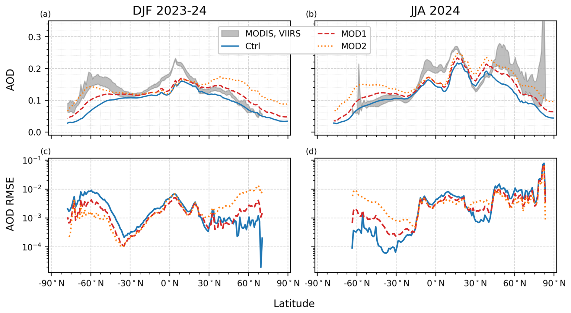
Figure 12 Zonal mean (a, b) and zonal RMSE (c, d) of seasonal 550 nm AOD during the DJF 2023–2024 season (a, c) and the JJA 2024 season (b, d). The grey shaded region is bounded by the AOD values calculated from MODIS and VIIRS, while the solid, dashed and dotted lines represent respectively the output of the control (Ctrl) and the simulations with modified wet-scavenging MOD1 and MOD2. The RMSE is calculated with respect to the mean of the MODIS and VIIRS AOD values. We included only points over the ocean, where the MODIS pixel count for AOD was larger than 150 and VIIRS had at least 7 d of valid retrievals.

As a final global evaluation of the sensitivity experiments, Fig. 12 shows the evaluation of zonal-mean 550 nm AOD and zonal RMSE against MODIS for the experiments. The largest impact of MOD1 and MOD2 is at mid- and high latitudes towards increased aerosol burdens, with up to ≈0.05 increase for MOD2. This leads to a significant reduction in zonal RMSE for the summer hemisphere by up to $\approx -\mathrm{0.1}$, and increased by the same amount over the winter hemisphere.

7 Discussion

We open this section by discussing overall limitations and performance of the N_d optimisation, and the magnitude of observational biases relevant to the optimisation results. Next, we focus on two discussion streams: one concerns the tendency of the model (partially mitigated with optimisation) to simulate N_d biased toward the upper bound of the uncertainty range; the other deals with the systematically low N_d at mid- and higher latitudes in the Southern hemisphere, where the optimisation is unable to bring improvement, and how the outcome of the sensitivity tests compare with the optimisation results. In both cases, results from the different setups (InCloud, InCloudNoBC, ClBase3), combined with independent observations, are used to clarify to what extent the optimal PSDs are consistent with independent observational constraints, and when they compensate for non-tuned aspects such as speciation, ageing or poor representation of aerosol mass concentrations.

7.1 Limitations and effectiveness of the N_d optimisation

While the magnitude of the reduction of ℒ by only 13 % may raise doubts about the effectiveness of the optimisation, it actually indicates that the prior (CAMS default) PSDs yield N_d values already close to the optimisation target. The main limitations of the optimisation lie in the prescribed spatial aerosol patterns from the model fields, and the restricted number of free parameters (the PSD r_med for five species). This is illustrated by the ClBase3 optimisation setup, where the prior N_d prediction has much larger errors throughout the tropics; in this setup, the improvement brought by the optimisation is significantly stronger, with a reduction of ℒ by 21 %.

The optimised (InCloud) SU median radius r_med is close to the prior 0.11 µm, keeping the increase in particle number below 11 % and the optical effect non-detectable. This PSD description was independently updated in IFS-COMPO CY49R1 (from r_med=0.0355 µm and σ=2.0) and we found that using the old PSD led to significantly larger number concentrations of activated SU by up to a factor ×2.7 (not shown), which the optimisation would then need to correct. While the new prior SU performs fairly well globally, observations of tropical marine sulfate aerosol have indicated mass transfer from Aitken (r≈0.04 µm) to accumulation (r≈0.1 µm) mode (Hoppel et al., 1990). However, the IFS-COMPO does not currently represent changes in aerosol PSDs over time, and in general no transfer of mass across bins is allowed (ECMWF, 2024a). Other models like the Met Office Unified Model do represent Aitken and accumulation modes for sulfate, and assess typical local mass ratios of 1 : 9 (Jones et al., 2001; Mulcahy et al., 2014). This variability in sulfate PSD may contribute the pattern of simulated N_d over the oceans, with high N_d biases over subsidence regions, and neutral-to-low in convective regions, indicating a potential benefit of an additional Aitken aerosol mode, either as sulfate or internally-mixed aerosol.

The fixed mass wet scavenging coefficients used by the IFS (between 0.7 and 0.9) for most hydrophilic species tend to be smaller than the typical mass activation rates close to unity provided by the activation scheme. Therefore, we performed an online IFS-COMPO simulation (setup as for simulations in Sect. 6) using scavenging rates diagnosed from the activation scheme and found the resulting changes in total aerosol mass to be within 5 % for SS, SOA, SOB, within 10 % for OM, and within 15 % for SU and NI species (see Appendix C). For most species (SS, SU, AM, OM) the resulting reduction in aerosol burdens would tend to increase the prior N_d biases for the optimisation. For OM, however, these reductions are too small to explain the reduction by a factor ×0.08 to ×0.31 required by the optimisation.

7.2 Known biases in N_d retrievals

MODIS N_d retrievals are known to suffer from an optical penetration bias due to the assumption that the spectrally-retrieved r_e values are representative of the droplet PSD at cloud top, leading to overestimated N_d (MODIS 2.1 µm) retrievals between 20 % and 40 % for marine clouds. Bias-correction of retrievals has been shown to occasionally improve agreement with in-situ measurement campaigns, but implications on N_d budgets are still unclear (Gryspeerdt et al., 2022b). This translates to an upper-bound effect of 12 % in $N_{\mathrm{d}}^{-\mathrm{1}/\mathrm{3}}$ over marine regions within 30° latitude.

At latitudes higher than 60° N and 45° S our method struggles to sufficiently increase N_d to match observations. MODIS cloud retrievals are known to suffer from viewing geometry errors with large satellite and solar zenith angles (Maddux et al., 2010; Grosvenor and Wood, 2014), potentially degrading high latitude observations. According to Gryspeerdt et al. (2022b), at latitudes higher than 60° N_d are overestimated by 16 cm⁻³ or less, which is potentially significant over relatively pristine regions over the ocean, with typical retrieved N_d values between 75 and 100 cm⁻³. These effects are included in one of the sampling strategies (BR17) and contribute to the error bars that we assigned to the MODIS N_d observations.

7.3 Carbonaceous aerosols and N_d over Africa

The optimisation results highlight that carbonaceous (OM, BC) aerosols are important contributors to simulated N_d over Africa and, as such, require a more detailed discussion of their representation. Particles with radii < 15 nm are weakly activated into cloud droplets, especially when characterised by low hygroscopicity, as in the case of soot. Representing BC with the same PSD as pristine soot might overestimate the number of particles, but underestimate their activation rates. This is because such an approach implicitly neglects the property of soot to form large chain-like clusters (e.g. Teng et al., 2019), resulting in a reduction of the effective number of independent particles available for activation. At the same time, this approach cannot represent the growth of such clusters into larger structures incorporating SU or OM particles (e.g. Yu et al., 2019), making them more efficient CCN providers. In addition, sensitivity of the activation efficiency to updraft velocity is expected in such aerosol-rich regimes; this sensitivity highlights both the relevance of ongoing efforts to better characterise updraft variability in global models (e.g. Ahola et al., 2022) and the difficulty of applying alternative approaches in our offline framework. However, updraft velocity plays a secondary role compared to aerosol number in determining the N_d bias, therefore the discussion will focus on the aerosol-related processes.

For black carbon CCN (defined as soot in Table 2), the median simulated number activation rate is around 0.5 %. If BC were represented in the form of aged aggregates of hundreds to thousands of monomers often incorporating organics and sulfate crystals, this would imply a reduced total amount of aggregates by two to three orders of magnitude which, however, readily activate due to internal mixing with larger and more hydrophilic particles. Moreover, BC ageing is an open area of research, and future work is needed to better characterise the role and relevance of aged BC and its representation on CCN simulations.

Sensitivity calculations of simulated optical properties (AOD, AE, spectra) indicate that the optimal PSD for OM is likely compensating for processes not represented in the optimisation. In fact, the optimised (InCloud) PSD visibly degrades the shapes of the aerosol size spectra and worsens the low bias in total column number concentrations (Fig. 7). The fact that InCloudNoBC produces N_d of similar quality, but with a neutral impact on aerosol optics, suggests that the compensated biases are related to the co-existence of BC and OM aerosol. Additionally, most of the aerosol counts from AERONET spectra are significantly higher than the model and associated with the fine-mode part of the size distribution (r⪅0.15 µm), which corresponds to BC in the model. However, a precise evaluation in this fine size regime is limited by the quickly decaying sensitivity (Dubovik and King, 2000) of the retrieval for r<0.1 µm, where the number contribution to CCN aerosol particles increases. However, the substantially flatter tail of the model spectra is consistent with the above-discussed limitations in the representation of OM and BC ageing.

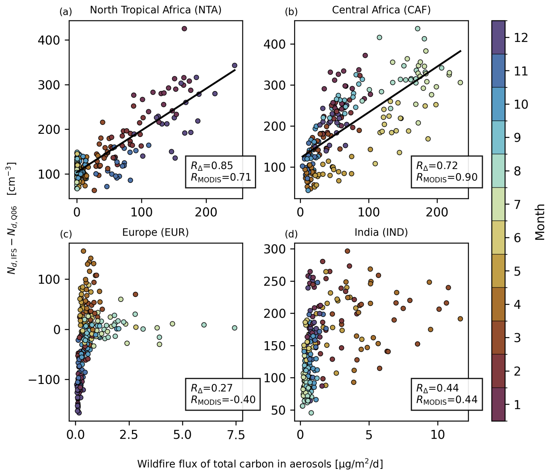
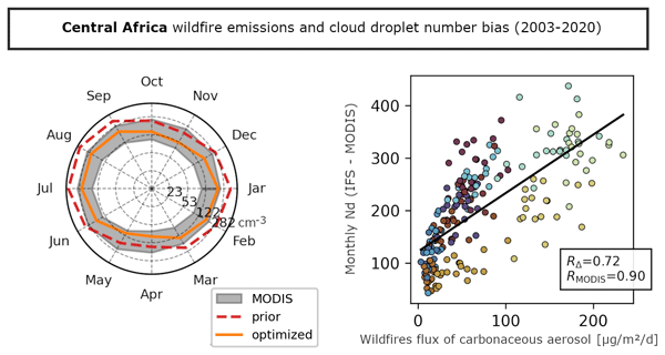
Figure 13 Scatter plot of wildfire flux of total carbon in aerosols (WFTCA) from the GFAS system and differences between simulated and MODIS “Q06” monthly N_d (2003–2020). R_Δ and R_MODIS indicate the Pearson's correlation coefficients between WFTCA and respectively, the difference $\mathrm{\Delta }=N_{\mathrm{d},\mathrm{IFS}}-N_{\mathrm{d},\mathrm{Q}\mathrm{06}}$ (R_Δ), and N_d,Q06 (R_MODIS).

In the IFS-COMPO, carbonaceous aerosol emissions are controlled by satellite observations of wildfires (Kaiser et al., 2012) via the Global Fire Assimilation System (GFAS). Figure 13 shows that wildfire carbonaceous aerosol emissions from GFAS correlate well with observed N_d in both regions (normalized covariance of 0.71 and 0.90) and the difference between observed and simulated N_d (normalized covariance of 0.85 and 0.72) for the north tropical Africa (NTA) and central Africa (CAF) regions, mirroring the seasonal biases in model N_d of Fig. 5. This does not hold for other regions like India (IND) and Europe (EUR), where wildfires are instead a weak predictor of N_d. The seasonality of N_d over NTA and CAF, and downstream over the mid-Atlantic, can therefore be associated with simulated wildfire emissions. This opens the possibility of using these results to support validation of related processes under active development for the wildfire assimilation systems, such as representation of wildfire types (Forkel et al., 2025) and associated smoke plumes.

We tested the robustness of the optimisation by excluding BC from the CCN calculations (InCloudNoBC). The rationale behind this is that the externally-mixed CAMS aerosol representation for this species is unsuited for describing the process by which BC is mostly scavenged in aggregated form with other, more efficient aerosol particles, and that therefore its contribution to the overall number of CCN is neutral. Results of the optimisation for this setup excluding BC from the CCN (labelled InCloudNoBC) are reported in Table 4 and are significantly closer to the prior definitions in the case of Org and Nit CCN providers. The almost identical final value of ℒ_InCloudNoBC to the InCloud setup indicates that excluding BC brings no significant change to the optimised N_d. Furthermore, the InCloudNoBC optimal PSD for OM has a nearly neutral effect on simulated OM AOD, which makes it a preferred option for its consistency with the current optical definitions; such a neutral impact can also be appreciated by visually comparing the typical mass extinction efficiency at r_med=0.09 µm and r_med=0.13 µm for OMH in Fig. 1. Given the equivalence of the resulting N_d, the higher consistency with OM aerosol optics and the significantly smaller size of the required LUT, InCloudNoBC emerges as a preferable configuration until CAMS BC representation is further improved.

The AE and AOD signal from SS aerosol (Fig. 12) strongly depends on the decision to keep the two SS PSD modes geometrically spaced by a factor 10 (see Table 1). The rigid displacement of the entire bimodal SS PSD towards smaller sizes during the optimisation is therefore driven by the number values associated with Ssf, for which the mass contributions from SS1 and SS2 are typically 70 % and 30 %. By design, Ssc provides extremely low CCN number concentrations (order of the unit against a background of dozens to hundreds cm⁻³); moreover, its role in reducing the activation efficiency of smaller, less hygroscopic particles, that we quantified within 15 %–20 % in the subtropical stratocumuli (not shown), provides too weak a signal in the overall simulated N_d to allow independent constraint of Ssc during the optimisation. However, the beneficial impact of decreasing AE over the ocean between 45° N and 45° S indicates that the current representation is plausibly underestimating the optical contribution of the coarse SS aerosol particles, and potentially also their relevance during aerosol activation.

7.4 Aerosol scavenging in mixed-phase clouds and N_d over the Southern Ocean

Testing the activation scheme (InCloud optimisation) with online IFS-COMPO experiments shows a widespread and strong decrease (up to ≈35 W m⁻²) of reflected solar radiation at latitudes south of 45° S, covering all the Southern Ocean (SO). Since the IFS, like many global models (Bodas-Salcedo et al., 2014), generally underestimates the amount of reflected solar radiation over the SO, this signal directly translates into a significant degradation of TOA SW fluxes. The understanding that these regions are strongly characterised by mixed-phase, boundary-layer cloud regimes (McFarquhar et al., 2021) motivated sensitivity tests targeting the aerosol wet removal for freezing clouds. For these clouds, air is typically supersaturated with respect to ice but subsaturated with respect to water, so that ice crystal growth occurs via deposition of water vapour produced by evaporating cloud droplets, a mechanism known as the Wegener-Bergeron-Findeisen (WBF) process (Pruppacher and Klett, 2010). From the standpoint of aerosols, this implies evaporation of activated CCN into interstitial cloud space, therefore limiting the efficiency of aerosol removal by precipitation compared to warm-phase clouds, where only liquid water is present.

Based on observations at one station in the Swiss Alps, Verheggen et al. (2007) produced two parametrisations to modulate scavenging efficiency in mixed-phase clouds, one temperature-dependent and the other phase-dependent, ζ(T) and ζ(IWR), to scale the activated number fraction of aerosol particles with diameter larger than 100 nm. Since the IFS IN-SCAV scheme already applies ζ(T) to rescale the mass-scavenging rates whenever snow is produced (ECMWF, 2024a), we experimented with two model changes adding complexity to the IN-SCAV scheme; the first uses a phase-dependent parametrisation of scavenging efficiency for both liquid and ice phase (MOD1); the second explicitly treats mixed-phase conditions and riming processes (MOD2).

When evaluating global TOA SW biases, the MOD1 and MOD2 setups still increased STDE relative to control, but this degradation was significantly smaller than that of InCloud (default IN-SCAV scheme) respectively, by 52 % (MOD1) and 86 % (MOD2). In the MOD1 and MOD2 experiments relative to the standard InCloud setup, the SW flux change is dominated (more than 90 %) by reduced cloud r_e because of higher diagnosed N_d by the activation scheme over the SO. This response is driven both by increased SS and SU aerosol burden (and associated AOD) at high latitudes, and by their longer persistence inside ice-precipitating clouds. Because no new optimisation was applied to MOD1 and MOD2 setups, the radiative response reflects the impact of the modified wet removal processes. The increased aerosol burden improves agreement in aerosol total-column number concentrations for most high-latitude AERONET sites, but tends to progressively overestimate AOD and underestimate AE, suggesting that the model is overestimating the size of aerosol particles at those locations.

The increased aerosol loads for MOD1 and MOD2 significantly improve AOD with respect to satellite observations over the summer hemisphere, but lead to a significant overestimation over the winter hemisphere, indicating a failure in capturing the seasonal variability of aerosols over marine mid- and high-latitudes. A possible explanation is that the IFS, despite linking SU production to the oxidation of available dimethyl sulfide (DMS), has no representation of sea-borne marine organic aerosols. These are likely linked to photosynthetic activity of phytoplanktons (Sellegri et al., 2024) and are found to significantly contribute to spatio-temporal variability of cloud N_d (McCoy et al., 2015). Therefore, considering sea spray as containing only SS might result in an overestimated burden of SS, with boundary layer aerosols lacking the correct seasonal cycle.

The MOD1 and MOD2 tests have demonstrated high sensitivity of simulated N_d to the representation of aerosol removal by precipitation from mixed-phase clouds. However, particles released by evaporating droplets also incorporate information on microphysical processes occurring before evaporation, e.g. collection, collision-coalescence or nucleation, resulting in internal mixtures with increased particle size (Hoose et al., 2008). Such evolution cannot be effectively represented with the single-moment cloud scheme of the IFS, since no memory of cloud particle number concentrations is preserved. Nonetheless, our investigation indicates that this is a plausible process limiting the effectiveness of the N_d optimisation at mid- to high latitudes.

The optimal N_d values from the ClBase3 optimisation perform markedly better than those from InCloud at mid- and high southern latitudes. This likely does not reflect better physical realism, because of the inconsistency with vertical tracer transport to cloud top (see discussion in Sect. 5), but rather a more meridionally uniform aerosol background found below cloud base than inside the cloud. To illustrate this point, Fig. 14 shows the amount of diagnosed Ssf particles (represented with the prior PSDs) during the InCloud and ClBase3 setups. In principle, low Ssf number concentrations are expected, as sea-spray is a secondary CCN provider (e.g. McFarquhar et al., 2021). However, coarse sea salt significantly impacts N_d in pristine regions via activation competition mechanisms of heterogeneous aerosol populations (Fossum et al., 2020), making a realistic representation of marine aerosol profiles essential to predict N_d. While particle concentrations at cloud level are typically between ≈7 and ≈20 cm⁻³ at subtropical latitudes, these sharply fall below 5 cm⁻³ with increasing latitude. Such meridional contrast is not found when diagnosing Ssf CCN just below the cloud base (with significantly higher values up to ≈30 cm⁻³), so that for ClBase3 their concentrations over the SO are of similar or higher magnitude than subtropical values. As a result of this substantially different aerosol background, the optimisation for ClBase3 yields significantly better agreement, although it does not guarantee physical consistency, highlighting the need for independent observational constraints. Nonetheless, this makes the ClBase3 approach a viable workaround for improved model N_d in IFS-COMPO until aerosol concentrations inside clouds are improved, with the important caveat of a trade-off between correcting N_d biases and preserving consistency with optics and vertical transport of tracers.

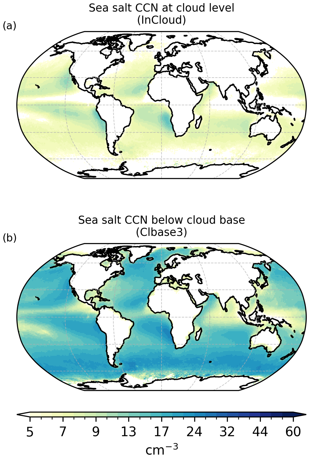
Figure 14 Mean N_d from sea salt fine (Ssf) CCN diagnosed during the offline optimisation procedure (2003–2020). The panels show aerosol diagnostics at cloud level (InCloud, a) and three model levels below cloud base (ClBase3, b), highlighting the different meridional distribution of diagnosed Ssf in the two setups.

8 Summary, outlook and conclusions

In this study, we introduced an explicit representation of aerosol-cloud interactions (ACI), limited to aerosol activation and the first indirect effect, in the ECMWF Integrated Forecasting System (IFS), enabling cloud droplet number concentrations (N_d) to be used as an additional aerosol diagnostic. By combining a physically informed aerosol activation scheme with 18 years of satellite N_d retrievals from MODIS, we showed that N_d can provide additional constraints on aerosol number concentrations for the Copernicus Atmosphere Monitoring Service (CAMS). Using this framework, we illustrated that a bulk aerosol scheme can reproduce broad large-scale patterns of N_d, within limits imposed by the aerosol size distributions (PSDs), vertical transport and wet removal processes.

We optimised the PSDs of CCN-providing aerosols using an offline diagnostic method, adjusting a small set of five free parameters using MODIS N_d observations. This method accounts for the co-location of aerosol and cloud profiles by combining stored output of prognostic aerosol simulations with reanalysis data, and consistently filters the same cloud regimes as in the N_d observations. The resulting effective PSD parameters substantially improve simulated N_d within the diagnostic framework used here, while having only a limited impact on aerosol optical properties. The optimised PSDs were further evaluated against independent observations of optical properties from AERONET and satellites.

The optimisation procedure was unable to correct low N_d at high latitudes over the ocean, especially over the Southern Ocean, leading to a degradation in simulated top-of-atmosphere (TOA) all-sky shortwave (SW) fluxes in online simulations. By performing online sensitivity tests, we showed that the simulated Southern Ocean N_d are highly sensitive to the representation of aerosol wet scavenging in mixed-phase clouds. Reduced scavenging efficiency in these regimes increases CCN concentrations within the clouds, offsetting most of the TOA SW degradation.

Despite a substantial reduction of the strong high-N_d bias over tropical Africa, the optimised N_d still show residual positive biases, although within the estimated observational uncertainty. Both observed and modelled N_d during periods of maximum residual bias are strongly correlated with carbonaceous emissions from assimilated wildfires in the model. Moreover, the optimal PSD returned for organic matter (OM) aerosol is inconsistent with independent AERONET observations over tropical Africa. This likely reflects limitations in the model representation of black carbon ageing processes, which do not capture the clustering over time of soot particles into larger, internally-mixed aerosol. Excluding black carbon from the optimisation yields comparable N_d, without degrading aerosol optical properties.

These results indicate that improving the consistency of simulated N_d at mid- and high-latitudes over pristine marine environments requires improved aerosol availability at cloud level. Excessive wet removal of aerosols in mixed-phase clouds emerges as a key regulator of aerosol indirect effects in the region, indicating a possible area for development in the CAMS aerosol system. Future improvements should also address deficiencies in the representation of marine aerosol sources, speciation and seasonality, including the potential role of biogenic primary marine organic aerosol. In the tropics, the results highlight the need to further constrain carbonaceous aerosol emissions and ageing, to better represent the impact of wildfire emissions on cloud microphysics. Future work will also be needed to address updraft variability relevant for aerosol activation in updraft-limited regimes, which is currently poorly constrained by observations.

As a final perspective, improving aerosol-cloud interaction representations in bulk aerosol schemes will require coordinated advances across multiple aspects of aerosol representation and associated processes. At the same time, satellite N_d observations emerge from this study as a valuable diagnostic tool that, combined with multi-spectral aerosol observations from ground-based photometers and satellite imagers, can help constrain aerosol number concentrations and associated processes that are only weakly informed by standard AOD validations.

Appendix A: Conversion from mixed bulk-bin representation to split bulk representation of sea salt aerosol

CAMS Sea salt aerosol is represented by a bimodal distribution whose domain is partitioned into three size intervals (bins), associated with a separate tracer (fine, medium, coarse – bins 1 to 3). For use in the activation scheme, a mapping from the mixed bulk-bin to a bulk monomodal representation is required.

In general, such conversion does not preserve all moments of the distribution, since the mixed bulk-bin representation allows discontinuities at bin boundaries. In this study, we map the three bins onto the two modes of the original bimodal distribution, thereby defining two sea salt species.

Let $n_i\left(r\right)=\mathrm{d}{N}_i/\mathrm{d}r\left(r\right)$ the ith mode of the original number PSD, α_i the relative weight assigned to the mode (${\sum }_i{\mathit{\alpha }}_i=\mathrm{1}$) and Φ_b the size interval of the bin b. The total mass of a bin b is given by:

$$\begin{array}{}\text{(A1)}& M_b=\sum _i{M}_{b,i}=\sum _i{\displaystyle \frac{\mathrm{4}}{\mathrm{3}}}\mathit{\pi }\mathit{\rho }\underset{{\mathrm{\Phi }}_b}{\int }{r}^{\mathrm{3}}{\mathit{\alpha }}_i{n}_i\left(r\right)\mathrm{d}r\end{array}$$

where ρ is the mass density. By taking the ratio $q_{b,i}=M_{b,i}/M_b$ one knows which fraction of the mass of the bin species b must be assigned to the split ith mode of the original bimodal distribution.

While this approach conserves total mass by construction, it does not constrain particle number concentrations, except for the special case where the relative bin mass contributions lead to a smooth merged distribution.

Appendix B: Relationship between AOD and particle number concentration in a bulk representation

The optical thickness per unit mass, here denoted by t, for an aerosol species with total mass M_a, is given by

$$\begin{array}{}\text{(B1)}& t\equiv \mathit{\tau }/M_{\mathrm{a}}=\mathit{\pi }{\displaystyle \frac{N_{\mathrm{a}}}{M_{\mathrm{a}}}}\int r^{\mathrm{2}}{Q}_{\mathrm{ext}}n\left(r\right)\mathrm{d}r\end{array}$$

where N_a is the total number of aerosol particles, n(r) is the normalized number distribution and Q_ext the Mie extinction efficiency. In the limit of narrow distributions, and for purely real refractive index, we can replace Q_ext with a local approximation dominated by a term ≈q r^k, with q and k real numbers. In the Rayleigh scattering regime k≈6; at the Mie resonance peak q≈4 and k≈0; in the geometric optics regime q≈2 and k≈0. Using standard expressions for the moments of the log-normal distribution n(r) yields

$$\begin{array}{}\text{(B2)}& \begin{array}{rl}t& \approx {\displaystyle \frac{q}{\mathrm{4}/\mathrm{3}\mathit{\pi }\mathit{\rho }}}{\displaystyle \frac{E\left[r^{k+\mathrm{2}}\right]}{E\left[r^{\mathrm{3}}\right]}}\\ & \approx {\displaystyle \frac{q}{\mathrm{4}/\mathrm{3}\mathit{\pi }\mathit{\rho }}}{r}_{\mathrm{med}}^{k-\mathrm{1}}{e}^{(k^{\mathrm{2}}+\mathrm{2}k-\mathrm{5}){\ln }^{\mathrm{2}}\mathit{\sigma }}\end{array}\end{array}$$

where r_med and σ are the median and geometric standard deviations of n(r).

The number of particles per unit mass, denoted by n_a, is obtained from the identity between total mass M_a and number of particles N_a:

$$\begin{array}{}\text{(B3)}& n_{\mathrm{a}}\equiv {\displaystyle \frac{N_{\mathrm{a}}}{M_{\mathrm{a}}}}={\displaystyle \frac{\mathrm{1}}{\mathrm{4}/\mathrm{3}\mathit{\pi }\mathit{\rho }}}{r}_{\mathrm{med}}^{-\mathrm{3}}{e}^{-\mathrm{9}{\ln }^{\mathrm{2}}\mathit{\sigma }}\end{array}$$

The number of cloud droplets is then a non-trivial but monotonic function of n_a, and is calculated by an activation scheme.

In a bulk representation, scaling the burden of an aerosol species proportionally affects τ and N_a. However, changes in r_med and σ affect t and n_a differently depending on the optical regime:

$$\begin{array}{}\text{(B4)}& {\displaystyle \frac{\partial t}{\partial \ln r_{\mathrm{med}}}}\approx (k-\mathrm{1})t\text{(B5)}& {\displaystyle \frac{\partial t}{\partial \ln \mathit{\sigma }}}\approx \mathrm{2}(k^{\mathrm{2}}+\mathrm{2}k-\mathrm{5})\ln \mathit{\sigma }t\text{(B6)}& {\displaystyle \frac{\partial n_{\mathrm{a}}}{\partial \ln r_{\mathrm{med}}}}=-\mathrm{3}{n}_{\mathrm{a}}\text{(B7)}& {\displaystyle \frac{\partial n_{\mathrm{a}}}{\partial \ln \mathit{\sigma }}}=-\mathrm{18}\ln \mathit{\sigma }{n}_{\mathrm{a}}\end{array}$$

In the limit r≪λ, Q_ext grows faster than linearly (i.e. k>1, with k=6 for the Rayleigh non-absorbing regime). In this case, increasing the median radius r_med decreases the optical thickness per unit mass t. For larger radii, q≈2, k≈0, so a smaller median radius leads to a larger optical thickness. Therefore, both the wavelength-to-size ratio and the refractive index determine how AOD responds to the particle size distribution.

Appendix C: Aerosol mass burden errors from activation rates in the IFS wet scavenging scheme

The IFS wet scavenging scheme assigns a prescribed dissolved mass fraction to each aerosol species: 0.9 for sea salt (SS), 0.8 for ammonium (AM) and nitrate (NI), 0.7 for all other hydrophilic species. However, the parcel model yields activated mass fractions close to 1 for most species except black carbon (BC), consistent with approaches adopted in global chemical transport models (see e.g. Wang et al., 2014b). The reason for this is that most aerosol species are dominated in mass by their large particle fraction, even for relatively low hygroscopicity species like organic matter (OM). In contrast, BC is characterised by substantial variability in activated mass fraction due to its low hygroscopicity and, most importantly, its typically small particle size. As a result, the IFS wet scavenging scheme is expected to underestimate aerosol removal for all species except BC. To quantify this effect, we performed an IFS-COMPO online experiment (with meteorology reinitialised every day from ERA5 and aerosols from previous day) for the period November-December 2023. In this experiment, the wet scavenging scheme diagnoses the dissolved mass fraction from the activation scheme rather than using the prescribed values. Figure C1 shows the global relative change in total column aerosol mass given by a simulation when wet scavenging rates are diagnosed from the activation scheme. The magnitude of the reduction remains typically within 15 %, overall confirming that the IFS wet scavenging scheme underestimates removal rates, but with a limited global impact.

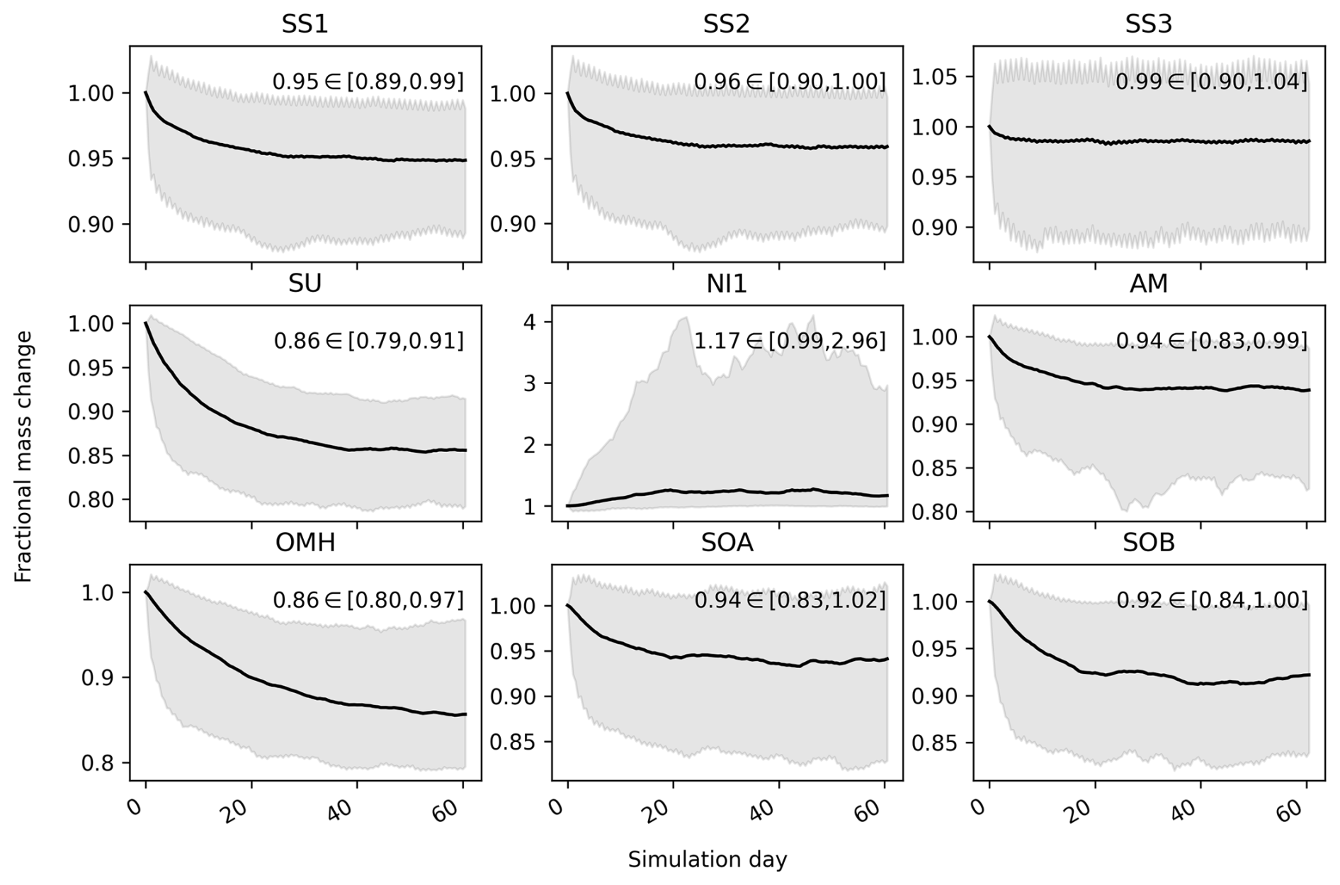
Figure C1 Relative change in total-column aerosol mass of several species from using in-cloud scavenging rates diagnosed by the aerosol activation scheme instead of the default fixed IFS values. Solid line is the median relative change (experiment divided by control), shadings are the global 5th and 95th percentiles of the relative change. For each panel, values for the last time-step (day 60) are reported.