Arctic sea ice loss amplifies local evaporation influence on water vapor isotopes: insights from cruise observations

Rapid Arctic warming and sea ice retreat have increased atmospheric humidity, yet the relative contributions of local evaporation and advected lower-latitude moisture remain poorly quantified. Here, we present high-resolution, ship-based in situ measurements of near-surface water vapor isotopes across diverse Arctic sea ice regimes between 17 July and 23 September 2024. By integrating isotope fractionation models with multi-source meteorological data, we show that sea ice changes act as a key modulator of Arctic water vapor isotopic variations. Under ice-covered conditions, water vapor isotopes are strongly temperature-dependent, exhibiting depleted δ¹⁸O and elevated d-excess due to Rayleigh-dominated long-range transport. As sea ice retreats, kinetic fractionation from local evaporation becomes increasingly important, particularly at temperatures above ∼5 °C, generating enriched δ¹⁸O, elevated d-excess, and a characteristic inverse isotope–temperature relationship. A Bayesian isotope mixing model quantifies the resulting moisture source shift, showing local evaporation contributions rise from 18.6 % (95 % CI: 11.1 %–40.9 %) in ice-covered regions to 43.8 % (95 % CI: 14.7 %–65.7 %) in ice-free regions, despite advected moisture remaining predominant. These findings provide a process-based isotope framework for the Arctic hydrological cycle, complementing conventional meteorological diagnostics and offering valuable observational constraints for interpreting paleo-isotope archives.

1 Introduction

Stable water vapor isotopes (δ¹⁸O and δD) and their derived deuterium excess (d-excess, defined as $\mathit{\delta }\mathrm{D}-\mathrm{8}\times \mathit{\delta }{}^{\mathrm{18}}\mathrm{O}$) are widely used as tracers for investigating hydrological processes and identifying moisture sources (Gat, 1996). These isotopes fractionate during phase transitions such as evaporation, condensation, and sublimation, encoding information about environmental conditions both at the moisture source and along the atmospheric transport pathways (Dansgaard, 1964; Galewsky et al., 2016; Bowen et al., 2019). As such, analysis of these isotopic parameters in modern water vapor and paleoclimate archives provides key insights into moisture sources and climatic dynamics across both modern (Kurita, 2011; Kopec et al., 2016; Wang et al., 2023) and paleoclimate contexts (Klein and Welker, 2016; Opel et al., 2013; Porter et al., 2019). This dual perspective is particularly critical in the Arctic, which serves not only as a modern laboratory of rapid hydrological change but also as a primary archive of past climate preserved in its ice sheets.

Recent Arctic amplification and sea ice loss have moistened the Arctic atmosphere (Min et al., 2008; Bengtsson et al., 2011; Bintanja and Selten, 2014), yet the relative roles of local evaporation and poleward moisture transport remain contested. Some studies attribute these changes to enhanced local evaporation over newly melt ocean (Bintanja and Selten, 2014; Boisvert and Stroeve, 2015; Kopec et al., 2016), while others emphasize strengthened poleward transport of lower-latitude moisture (Bengtsson et al., 2011; Zhang et al., 2013; Zhong et al., 2018). Resolving this debate is crucial because water vapor plays a central role in Arctic radiative and hydrological feedbacks, influencing cloud cover, precipitation, and surface warming. Stable water vapor isotopes provide a process-based diagnostic for disentangling and quantifying the relative contributions of these two sources. Such insights are essential not only for improving the representation of hydrological processes in climate models, thereby enabling more reliable projections (Barras and Simmonds, 2009; Gao et al., 2011; Sturm et al., 2010; Xi, 2014), but also for interpreting isotopic signals preserved in paleoclimate archives such as ice cores (Klein et al., 2016; Opel et al., 2013; Porter et al., 2019).

However, the application of stable isotopes in the Arctic remains challenging due to conflicting interpretations of isotopic signals, particularly regarding the role of local evaporation. One line of evidence associates high d-excess and low δ¹⁸O over open water with strong evaporation under cold, dry air masses, as observed in both water vapor (Kurita, 2011; Steen-Larsen et al., 2013; Bailey et al., 2021) and precipitation (Mellat et al., 2021). In contrast, Klein et al. (2015) proposed that local evaporation associated with sea ice loss leads to enriched δ¹⁸O and suppressed d-excess in Arctic water vapor, relative to advected lower-latitude moisture, a pattern that is also reflected in observed Arctic precipitation (Kopec et al., 2016; Song et al., 2023). However, this interpretation is further complicated by recent evidence showing that low-latitude moisture can also produce low vapor d-excess when influenced by synoptic-scale extratropical cyclones (Thurnherr and Aemisegger, 2022). These divergent interpretations largely reflect the scarcity of spatially extensive, high-resolution vapor isotope observations across the Arctic Ocean. Most existing studies are based on land-based observations, with limited coverage over the Arctic Ocean, hindering efforts to disentangle complex isotope signals (Kurita, 2011; Kopec et al., 2016; Mellat et al., 2021). Klein and Welker (2016) suggested the relative influence of local evaporation on water vapor isotopes may vary with sea ice extent (SIE), proposing an anti-correlation between d-excess and SIE. However, subsequent studies have reported the opposite relationship (Bonne et al., 2019). This persistent inconsistency underscores the need for broader, in-situ water vapor isotope observations across different sea ice regimes.

To address this gap, we leverage a new set of high-resolution, in-situ water vapor isotope measurements obtained during a comprehensive summer expedition across the Arctic Ocean aboard the RV Xuelong 2. This dataset provides extensive spatial coverage across the Arctic, spanning sea ice regimes from near-continuous cover to open water. By integrating these isotopic observations with meteorological data, and applying isotope-based diagnostics along with Lagrangian trajectory analysis, this study aims to: (1) map the spatial patterns of summer Arctic vapor isotopes in relation to diverse sea ice regimes, (2) identify the primary mechanisms behind isotope variability under distinct sea ice conditions, and (3) quantify the partitioning between locally evaporated and advected moisture sources across different Arctic regions.

2 Data and Methods

2.1 Water Vapor Isotope Measurements and Calibration

Continuous, in situ measurements of near-surface water vapor isotopes and humidity were conducted using a Picarro L-2130i cavity ring-down spectroscopy (CRDS) analyzer. The instrument was housed in the meteorological laboratory aboard RV Xuelong 2 during China's 14th Arctic Scientific Expedition. The data were obtained between 17 July and 23 September 2024, during which RV Xuelong 2 transited the Arctic Ocean from the Bering Strait through the Chukchi Sea and the central Arctic Ocean to the Barents Sea, before returning to the Bering Strait via the East Siberian Sea (Fig. 1). Ambient air was drawn from an inlet mounted on the balcony of the meteorological room, approximately 10 m above sea level. The inlet was equipped with a hydrophobic polytetrafluoroethylene (PTFE) filter (Nanjing Liebo) to prevent particle contamination and icing during sampling. The sample air was delivered to the analyzer through a 5 m PTFE inlet tube. Most of the tubing was routed inside the meteorological laboratory, where air conditioning maintained the temperature at ∼20 °C, preventing condensation without additional heating.

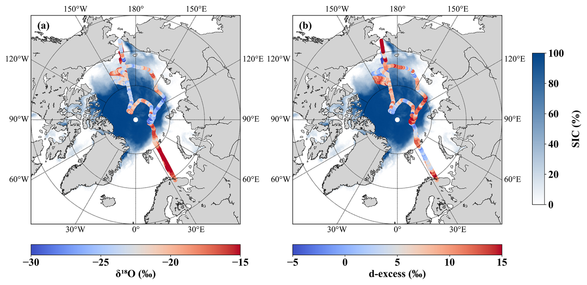
Figure 1 Spatial distributions of water vapor δ¹⁸O (a) and d-excess (b) along the cruise track. Colored dots indicate measured isotopic values (‰) and shading shows the mean sea ice concentration (SIC) during the observation period.

All isotope values are reported in standard δ notation relative to the Vienna Standard Mean Ocean Water (VSMOW):

$$\begin{array}{}\text{(1)}& \mathit{\delta }=\left({\displaystyle \frac{R_{\text{sample}}}{R_{\text{VSMOW}}}}-\mathrm{1}\right)\times \mathrm{1000}\end{array}$$

where R_sample and R_VSMOW are the isotope ratios (${}^{\mathrm{18}}\mathrm{O}{/}^{\mathrm{16}}\mathrm{O}$ or ${}^{\mathrm{2}}\mathrm{H}{/}^{\mathrm{1}}\mathrm{H}$) of the sample and VSMOW, respectively. The measurement precision was 0.25 ‰/0.08 ‰ for δ¹⁸O and 1.6 ‰/0.5 ‰ for δD at 10 s/100 s averaging intervals, respectively. The long-term analytical reproducibility, estimated from repeated measurements of internal laboratory standards over the study period and derived from normalization residuals, was ±0.06 ‰ for δ¹⁸O and ±0.3 ‰ for δD (1σ). The data were originally collected at 1 min intervals and have been resampled to hourly resolution for analysis. D-excess was calculated following Dansgaard (1964) as:

$$\begin{array}{}\text{(2)}& \text{d-excess}=\mathit{\delta }\mathrm{D}-\mathrm{8}\times \mathit{\delta }{}^{\mathrm{18}}\mathrm{O}\end{array}$$

Because the isotope measurements from the Picarro analyzer are subject to ambient water vapor concentration, a humidity-dependent correction was applied to ensure consistency across varying atmospheric conditions. Calibration was performed using a Standard Delivery Module (SDM). To define the calibration gradient, we used the analyzer's internal humidity measurements, which closely agree with independent sensors (Wang et al., 2023; Bonne et al., 2019), without relying on external references. Following Liu et al. (2014), two VSMOW-standard water samples were analyzed at three flow rates (0.015, 0.04, 0.07 µL s⁻¹) to generate three humidity levels of 5000, 15 000, and 25 000 ppm, and each step was maintained for 20 min. A full calibration cycle was performed approximately every 22 h during atmospheric measurements. To minimize memory effects, the first 10 min and final 2 min of each calibration step were excluded. A correction function was derived from the valid calibration data to express isotope bias as a function of humidity and was applied to all samples to normalize their values to a reference humidity of 20 000 ppm:

$$\begin{array}{}\text{(3)}& {\displaystyle }\begin{array}{rl}{\mathit{\delta }}_{\text{measured}}& -{\mathit{\delta }}_{\text{humidity calibration}}=\\ & f\left({\text{humidity}}_{\text{measured}}\right)-f\left(\mathrm{20}\mathrm{000}\right)\end{array}\text{(4)}& {\displaystyle }{f}_{\mathit{\delta }{}^{\mathrm{18}}\mathrm{O}}\left(\text{humidity}\right)=\mathrm{0.2976}\ln \left(x\right)-\mathrm{11.969}\text{(5)}& {\displaystyle }{f}_{\mathrm{D}}\left(\text{humidity}\right)=\mathrm{0.2843}\ln \left(x\right)-\mathrm{30.892}\end{array}$$

Equations (4) and (5) describe the humidity-dependent isotope bias for δ¹⁸O and δD, respectively, derived from the calibration measurements. Equation (3) was used to correct all isotope measurements to a reference humidity of 20 000 ppm, thereby minimizing the influence of water vapor concentration on the measured isotope values.

All vapor isotope measurements were then normalized to the VSMOW scale using two laboratory reference waters ($\mathit{\delta }{}^{\mathrm{18}}\mathrm{O}=-\mathrm{11.02}$ %, $\mathit{\delta }\mathrm{D}=-\mathrm{78.1}$ ‰; $\mathit{\delta }{}^{\mathrm{18}}\mathrm{O}=-\mathrm{29.86}$ ‰, $\mathit{\delta }\mathrm{D}=-\mathrm{222.9}$ ‰), whose isotope values match the expected range of water vapor isotopes in the Arctic. The certified uncertainties provided by the calibration laboratory were ±0.021 ‰ (δ¹⁸O) and ±0.530 ‰ (δD) for the first standard, and ±0.006 ‰ (δ¹⁸O) and ±0.104 ‰ (δD) for the second standard. Both standards were pre-corrected for humidity-dependent bias, and a linear calibration function was established based on the measured versus true values of the two standards and applied to all samples to complete the VSMOW normalization.

2.2 Meteorological and sea ice data

Meteorological data, including air temperature (T), relative humidity (RH), and air pressure, were obtained from the onboard weather station of the RV Xuelong 2, located in close proximity to the isotope inlet. Specific humidity (q) was calculated from the water vapor concentration measured by the Picarro instrument. All datasets were synchronized to the isotope measurement timestamps (UTC+8) and averaged to 1 min resolution. Surface evaporation flux (E), representing the instantaneous vertical water vapor flux from the ocean surface, was obtained from the fifth-generation European Centre for Medium-Range Weather Forecasts reanalysis (ERA5; Hersbach et al., 2023), available at 1 h temporal and 0.5°×0.5° horizontal resolution.

The daily 4 km sea ice concentration (SIC) data were obtained from the National Snow and Ice Data Center (NSIDC), specifically from the MASIE-AMSR2 (MASAM2) blended product (Fetterer et al., 2023). This product integrates data from the Multisensor Analyzed Sea Ice Extent (MASIE) and the Advanced Microwave Scanning Radiometer 2 (AMSR2). To assess the influences of sea ice on water vapor isotopes and moisture source partitioning, the Arctic was classified into three sea ice regimes using contemporaneous SIC data (Fig. 2):

• I.

  Ice-free Region (SIC<0.4): areas below satellite detection threshold (MASAM-2 SIC=0)

• II.

  Sea Ice Region (SIC>0.85): predominantly ice-covered areas

• III.

  Transition Region ($\mathrm{0.4}\le \text{SIC}\le \mathrm{0.85}$): intermediate ice conditions

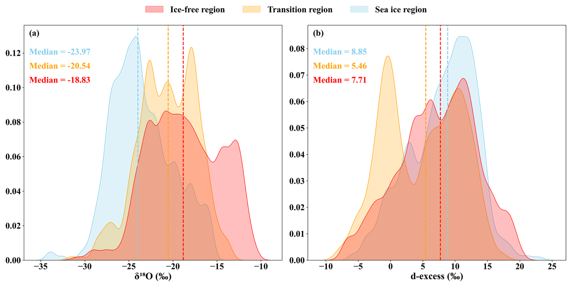
Figure 2 Probability density distributions of δ¹⁸O (a) and d-excess (b) in the sea ice Ice-free (red), Transition (orange), and Sea Ice (blue) regions. Median values for each region are indicated.

2.3 Theoretical Isotope Modelling of Ocean Evaporation

We employed the MJ79 model (Merlivat and Jouzel, 1979) to estimate the isotopic composition of water vapor evaporated from Arctic ocean, following the formulation of Bonne et al. (2019):

$$\begin{array}{}\text{(6)}& R_{\text{BL}}={\displaystyle \frac{R_{\text{SW}}}{{\mathit{\alpha }}_{\text{eq}}\times ({\mathit{\alpha }}_k+\text{RH}(\mathrm{1}-{\mathit{\alpha }}_k\left)\right)}},\end{array}$$

where R_BL is the isotopic ratio of water vapor in the boundary layer, and R_SW is the isotopic ratio of surface seawater. RH is the relative humidity at the sea surface. α_eq and α_k are the equilibrium and kinetic fractionation coefficients, respectively. α_eq was calculated as a function of temperature, while α_k takes values of 1.0060 for δ¹⁸O and 1.0053 for δD under smooth wind conditions, and 1.0035 for δ¹⁸O and 1.0031 for δD under rough wind conditions (Bonne et al., 2019). Because surface seawater isotope values in the open Arctic Ocean are typically close to 0 ‰ (Namyatov et al., 2024, 2023), we prescribed δ¹⁸O and δD of surface seawater as 0 ‰, from which R_SW was calculated and used as the model input.

2.4 Back-trajectory calculation

To identify moisture sources in the Arctic, we analyzed air mass trajectories using the Hybrid Single Particle Lagrangian Integrated Trajectory (HYSPLIT) model (Stein et al., 2015). The model was driven by 0.5°×0.5° Global Data Assimilation System (GDAS) meteorological fields from the National Oceanic and Atmospheric Administration (NOAA) Air Resources Laboratory.

Ten-day backward trajectories were computed hourly along the cruise track at five vertical levels (10, 20, 30, 40, and 50 m above the surface). This duration aligns with the typical residence time of atmospheric water vapor in polar regions (Gimeno et al., 2021; Wallace and Hobbs, 2006) and is long enough to capture moisture transport from lower latitudes. The selected vertical levels span the full range of the research vessel's measurements, enabling a more comprehensive representation of air mass histories. Building on these trajectory calculations, moisture-weighted source contributions from the Pacific and Atlantic sectors were quantified. All trajectories were batch-processed using the PySPLIT Python package (Warner, 2018).

2.5 Bayesian isotope mixing model

To quantify the contributions of different moisture sources to Arctic water vapor, we employed MixSIAR (Stock and Semmens, 2016a), an open-source Bayesian mixing model implemented in R. MixSIAR, developed from earlier MIXSIR and SIAR, has been widely applied in ecological and environmental studies. The model infers source contributions by representing each vapor isotope measurement as a mixture of multiple endmembers and exploring all feasible combinations of source proportions. Solutions that satisfy isotope mass balance within the uncertainty of both endmembers and observations are retained, forming the posterior distribution of source contributions. According to Stock et al. (2018), the model framework can be expressed as:

$$\begin{array}{}\text{(7)}& Y_j={\sum }_k{p}_k{u}_{jk}^s,\end{array}$$

where Y_j is the tracer value of the mixture for tracer j, p_k is the proportional contribution of source k, and $u_{jk}^s$ is the mean tracer value of source k. Given the substantial isotopic variability in Arctic water sources and its propagation into the vapor mixture, we evaluated three error structures (residual, process, multiplicative) and adopted the process error structure as most appropriate (Stock and Semmens, 2016b):

$$\begin{array}{}\text{(8)}& Y_{ij}\sim N({\sum }_k{p}_k{u}_{jk}^s,{\sum }_k{p}_k^{\mathrm{2}}{\mathit{\omega }}_{jk}^{s\mathrm{2}})\end{array}$$

where N represents the normal distribution and ω represents the source variance of the two stable isotope tracers. Posterior distributions were estimated using Markov Chain Monte Carlo (MCMC) sampling with the “Normal” run length setting (chain length = 100 000; burn-in = 50 000; thinning = 50; 3 chains), following the MixSIAR manual (Stock and Semmens, 2016a). Given the limited knowledge of moisture source partitioning in the Arctic, uninformative Dirichlet priors (α=1) were assigned to the source proportions, specifying equal prior probability for all potential source mixtures. Model convergence was assessed using the Gelman-Rubin diagnostic, with values below 1.05 indicating satisfactory convergence of the MCMC chains.

To construct a representative lower-latitude moisture end-member, trajectory statistics were performed using a custom Python script. Source end-member data were input as means and standard deviations. Air trajectories from Pacific (160° E–160° W) and Atlantic (15° E–30° W) were integrated and weighted by the specific humidity of each backward trajectory at the time it crossed the Arctic boundary (66.5° N). The weight W_k for each channel k was calculated as:

$$\begin{array}{}\text{(9)}& W_k={\displaystyle \frac{{\sum }_{i=\mathrm{1}}^{N_k}{q}_{i,\text{cross}}}{{\sum }_{\text{all}}{q}_{i,\text{cross}}}}\end{array}$$

where q_i,cross represents the specific humidity of trajectory i at the moment of crossing 66.5° N. The composite isotopic mean δ_mix was then derived using Eq. (10), and the mixed standard deviation σ_mix was calculated following the Gaussian error propagation rule (Eq. 11):

$$\begin{array}{}\text{(10)}& {\displaystyle }{\mathit{\delta }}_{\text{mix}}={\sum }_k(W_k\cdot {\mathit{\delta }}_k)\text{(11)}& {\displaystyle }{\mathit{\sigma }}_{\text{mix}}=\sqrt{{\sum }_k(W_k\cdot {\mathit{\sigma }}_k{)}^{\mathrm{2}}}\end{array}$$

A Rayleigh distillation correction was applied to the lower-latitude source end-member to account for isotopic depletion during poleward transport. The initial source region is defined as the North Pacific (50–60° N), with a saturation specific humidity of 6.6 g kg⁻¹ (corresponding to ∼8 °C). Using the weighted approach described above, initial δ¹⁸O and δD values of −17.68 ‰ and −134.4 ‰ were obtained. This air mass was modified according to a Rayleigh fractionation curve to a target humidity of 3.93 ± 1.84 g kg⁻¹, which represents the hourly mean saturation specific humidity across the Arctic domain resulting from rainout of lower-latitude water vapor along the trajectories. The calculated isotope values, representing the discrimination between the lower-latitude source and the Arctic background state due to Rayleigh fractionation, were incorporated into the MixSIAR model.

The local evaporation end-member was derived using hourly air temperature and relative humidity from shipboard observations in ice-free region as inputs for the MJ79 model (see Sect. 2.3), implemented via a Python script. The model was run in batch mode to calculate the isotopic composition of vapor due to local evaporation. The resulting means and standard deviations were used to define the local evaporation end-member in the MixSIAR model.

To assess the sensitivity of the inferred source contributions to endmember variability and prior assumptions, sensitivity analyses were conducted. For endmember selection, the isotopic compositions of both local and remote source endmembers were perturbed by ±20 %, corresponding to approximately ±1σ of the observed variability during the campaign, and 1000 randomized endmember sets were generated and propagated through the MixSIAR framework. For the Bayesian mixing model configuration, alternative Dirichlet priors were tested, including an uninformative prior ($\mathit{\alpha }=(\mathrm{1},\mathrm{1})$), a weakly informative prior ($\mathit{\alpha }=(\mathrm{2},\mathrm{2})$), and biased priors favoring each endmember ($\mathit{\alpha }=(\mathrm{3},\mathrm{1})$ and $\mathit{\alpha }=(\mathrm{1},\mathrm{3})$).

3 Results

3.1 Water Vapor Isotope Variability Along the Cruise Track

Figure 1 shows the evolution of near-surface water vapor isotopes and sea ice coverage along the trans-Arctic RV Xuelong 2 expedition track spanning the Chukchi Sea, central Arctic Basin, Barents Sea, and Laptev–East Siberian Seas, suggesting co-variability between them. δ¹⁸O exhibited a pronounced spatial gradient along the cruise track, with the most enriched values (−10.8 ‰) in the ice-free Barents Sea, gradually becoming depleted poleward to the most depleted values (−34.19 ‰) in the heavily ice-covered central Arctic (SIC>90 %), a pattern that inversely mirrors the gradient in sea ice coverage (Fig. 1a). This anti-phase variation between water vapor δ¹⁸O and sea ice coverage is further confirmed by the δ¹⁸O distributions across different sea-ice coverage regions (Fig. 2a), which reveal a systematic δ¹⁸O enrichment from the Sea Ice Region ($\text{median}=-\mathrm{23.97}$ ‰), through the Transition Region (−20.54 ‰), to the Ice-free Region (−18.83 ‰). These results suggest that sea ice changes may contribute to variations in water vapor isotope composition across the Arctic.

In contrast, the second-order parameter d-excess exhibits a more complex spatial pattern, with elevated values primarily observed both near coastal regions and in some localized zones of the ice-covered central basin (Fig. 1b). The highest values (23.31 ‰) were recorded in the central basin under steady sea ice cover, while the lowest (−8.35 ‰) occurred in the Chukchi Sea amid fluctuating sea ice (SIC varied from 40 % to 85 %). When grouped by SIC regimes, both the Ice-free and Sea Ice Regions sustained relatively higher d-excess values (median=7.71 ‰ and 8.85 ‰, respectively), whereas the Transition Region yielded the lowest values (median=5.46 ‰) (Fig. 2b). This different d-excess pattern across sea ice regimes points to the influence of sea ice changes on Arctic water vapor isotopic composition, likely through shifts in moisture sources and kinetic fractionation processes.

To examine how sea ice changes modulate Arctic water vapor isotopes, we show the variations of δ¹⁸O and d-excess in relation to temperature, humidity, and local evaporation along the cruise track (Fig. 3). A comparison across the three sea ice regimes reveals that δ¹⁸O and d-excess exhibited pronounced, anti-phase fluctuations (Fig. 3b). Depleted δ¹⁸O generally coincided with colder, drier air in the ice-covered central Arctic, while enriched values occurred in warm, moist sectors like the Barents Sea (Fig. 3d). The episodes of high d-excess were closely associated with conditions of reduced relative humidity and enhanced evaporation, particularly in the Ice-free Region (Fig. 3c), highlighting the enhanced influence of kinetic fractionation over open water. These co-variations demonstrate that the sea ice regimes set the boundary conditions for the atmospheric controls – from equilibrium (temperature-driven) to kinetic (evaporation-driven) – on Arctic water vapor isotopes.

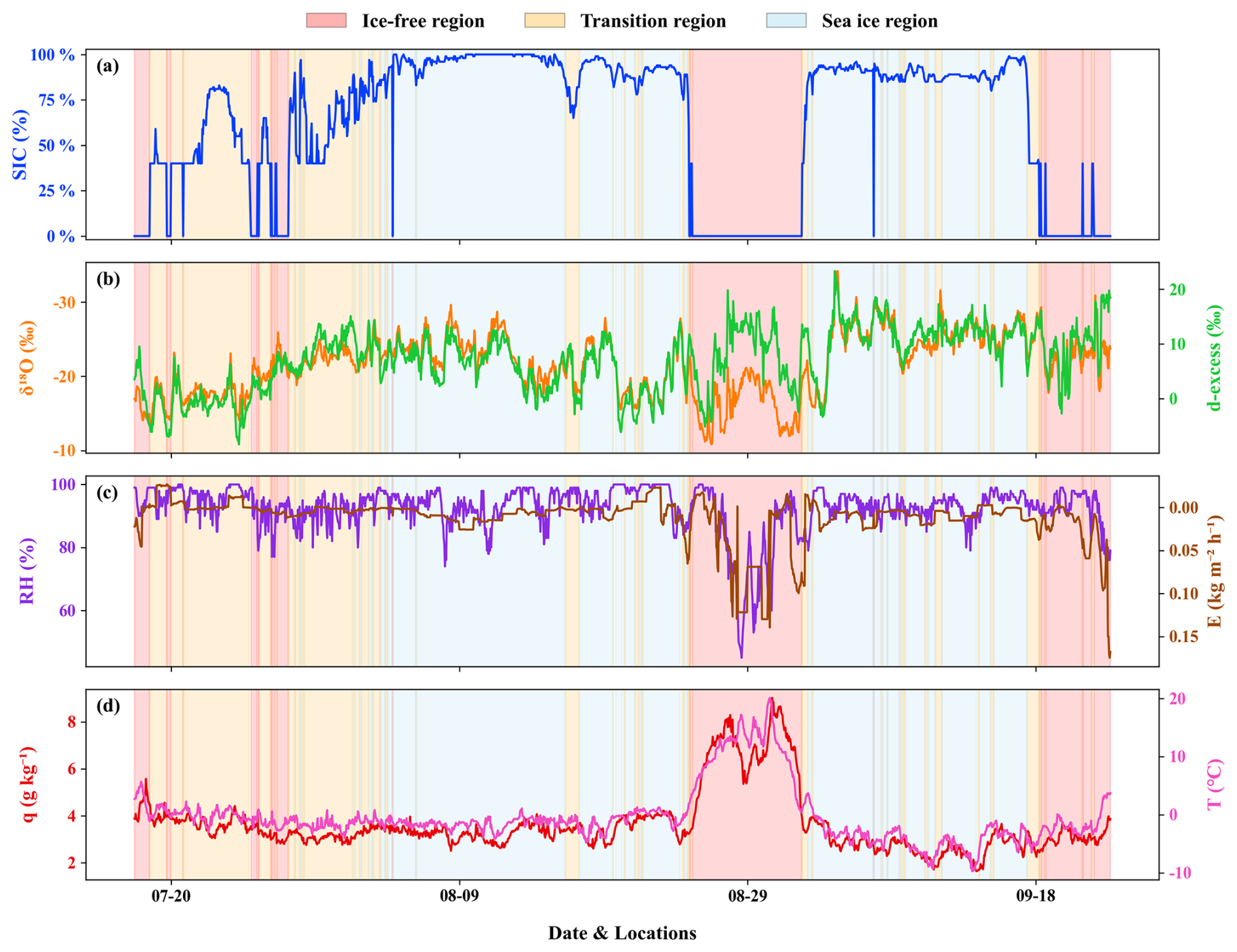
Figure 3 Temporal and spatial evolution of observed water vapor isotopes, SIC, and meteorological parameters along the cruise routes. (a) SIC (%); (b) δ¹⁸O (‰) and d-excess (‰); (c) Relative humidity (RH; %) and Evaporation (E; $\mathrm{kg}{\mathrm{m}}^{-\mathrm{2}}{\mathrm{h}}^{-\mathrm{1}}$); (d) Specific humidity (q; g kg⁻¹) and air temperature (T; °C). Background colors indicate the three different sea ice regimes.

3.2 Isotopic Responses to Temperature and Humidity across Arctic Sea Ice Regimes

To investigate isotopic responses to temperature and humidity, we first examined the relationship between δ¹⁸O and air temperature in the three distinct sea ice regions. As expected, δ¹⁸O values exhibit significant positive correlations with temperature in all regions (Fig. 4a), consistent with the classical “temperature effect” (Dansgaard, 1964). However, this relationship weakens notably in the Ice-free Region and reverses when temperatures exceed 5 °C, during which δ¹⁸O becomes negatively correlated with temperature, indicating a departure from equilibrium fractionation and the emergence of dominant kinetic processes under warm, ice-free conditions.

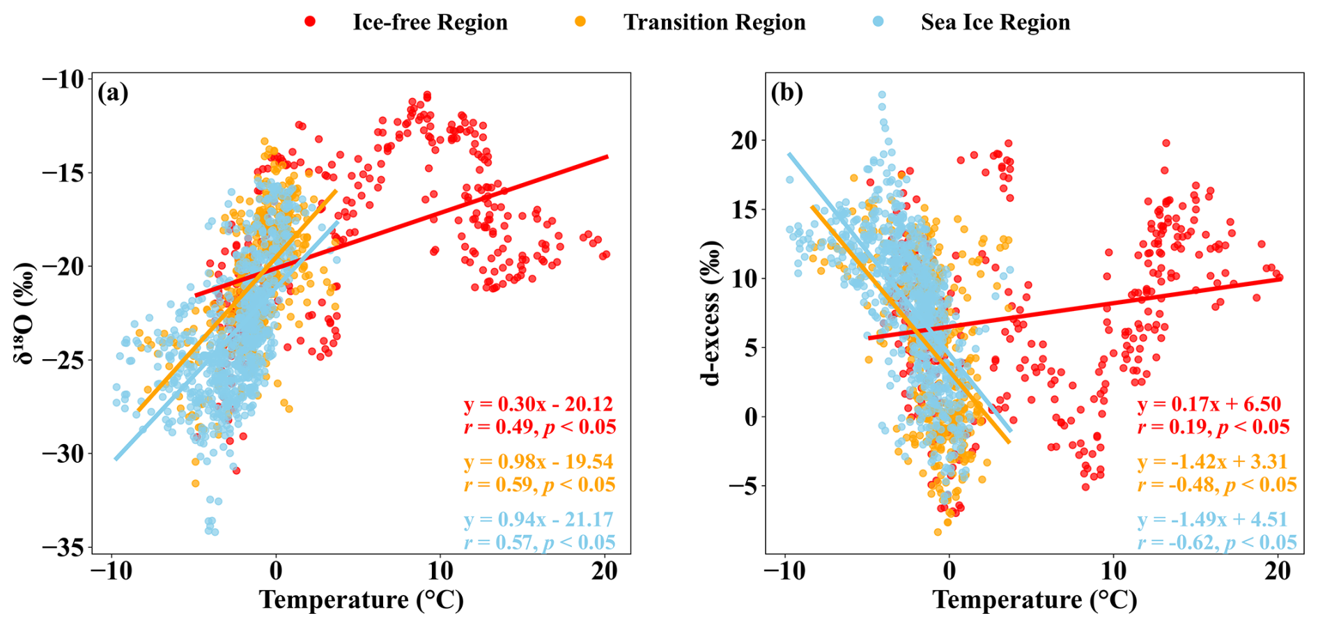
Figure 4 Relationships of water vapor isotopes with air temperature across three sea ice regimes. (a) δ¹⁸O versus temperature; (b) d-excess versus temperature. Dots and linear regression lines are color-coded by regime: ice-free (red), transition (yellow), and sea ice (blue). Regression statistics are displayed in corresponding colors.

In contrast, d-excess shows a more variable response to temperature. Significant negative correlations are observed in the Sea Ice and Transition Regions ($r=-\mathrm{0.62}$ and −0.49, respectively; p<0.05; Fig. 4b), whereas the Ice-free Region exhibits a weak positive correlation (r=0.19; p<0.05; Fig. 4b). In the Ice-free Region, the correlation shifts from negative to positive when temperature is above 5 °C, suggesting a shift in the dominant controls on isotopic variability. Although d-excess is theoretically not expected to directly depend on temperature (Shao et al., 2021; Xiang et al., 2022), previous studies have shown that a positive correlation can emerge as a signature of oceanic evaporation (Uemura et al., 2008). This suggests that correlation between d-excess and temperature may serve as a diagnostic of the influence of local evaporation on Arctic water vapor (Brunello et al., 2023). Collectively, these patterns indicate that fractionation mechanisms undergo fundamental shifts between ice-covered and open-water environments, with an enhanced role of kinetic effects over the ice-free ocean.

Relative humidity (RH) serves as a diagnostic of atmospheric sub-saturation, which controls the magnitude of kinetic isotopic fractionation during evaporation (Bonne et al., 2019). Across all sea ice regimes, d-excess exhibits a consistent negative correlation with RH (Fig. 5a), with the strongest correlation in the Ice-free Region ($r=-\mathrm{0.52}$, p<0.05), followed by the Transition ($r=-\mathrm{0.37}$) and Sea Ice Regions ($r=-\mathrm{0.33}$). A similar pattern is observed for the relationship between d-excess and surface evaporation (Fig. 5b), with the strongest positive correlation in the Ice-free Region (r=0.51) and weaker ones in the Transition (r=0.40) and Sea Ice (r=0.24) Regions. These results indicate that as sea ice retreats, local evaporation increasingly governs the isotopic composition of Arctic water vapor, consistent with the elevated d-excess observed in ice-free areas, while its influence remains relatively weak in ice-covered regions.

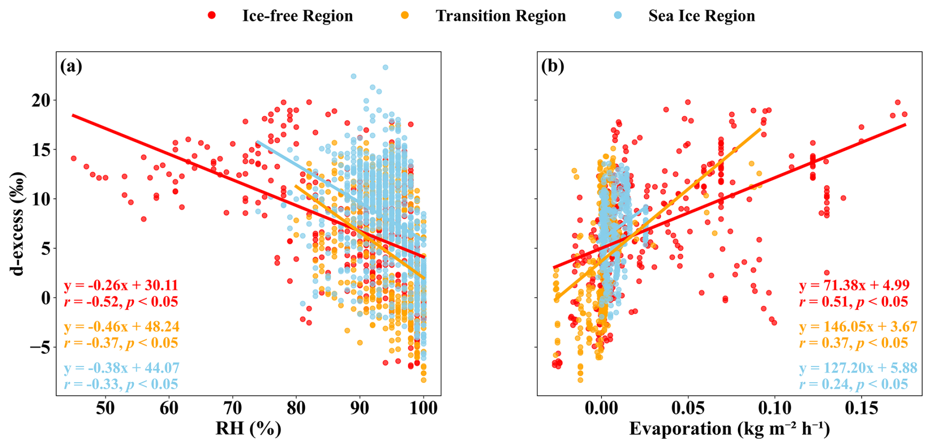
Figure 5 Relationships of d-excess with relative humidity and evaporation across three sea ice regimes. (a) d-excess versus relative humidity (RH); (b) d-excess versus evaporation flux. Dots and linear regression lines are color-coded by regime: ice-free (red), transition (yellow), and sea ice (blue). Regression statistics are displayed in corresponding colors.

3.3 Moisture Sources and Fractionation Processes across Arctic Sea Ice Regimes

To disentangle the influences of equilibrium and kinetic fractionation on Arctic water vapor isotopes, we employ q–δ diagrams as a diagnostic tool (Fig. 6a). Within a Rayleigh framework, δ¹⁸O decreases systematically as vapor is progressively depleted through condensation during long-range transport, whereas d-excess remains relatively constant (Worden et al., 2007; Galewsky and Samuels-Crow, 2015; Noone, 2012). In the q–δ diagram, the idealized Rayleigh process forms a reference curve along which data distributions reflect the dominant influence of equilibrium fractionation. Data points deviating from this trajectory indicate additional physical processes: values above the curve often reflect admixture with other air masses (Wang et al., 2023), those below the mixing line reflect interactions between air masses of contrasting humidity (Galewsky and Samuels-Crow, 2015), and points below the Rayleigh curve typically signify local evaporation, such as from rain or open water (Worden et al., 2007). To specifically diagnose kinetic effects, we also examine a q–d-excess diagram (Fig. 6b), accounting for realistic polar conditions with Rayleigh curves modified for ice supersaturation (RH_i=100 %–110 %). Under these conditions, kinetic fractionation suppresses d-excess below equilibrium predictions (Jouzel and Merlivat, 1984; Jensen and Pfister, 2005). Within this framework, points falling below the equilibrium curve primarily reflect d-excess suppression by ice-supersaturated cloud formation, whereas points above it indicate contributions from evaporation or sublimation (Samuels-Crow et al., 2014; Kopec et al., 2019). Collectively, these dual diagrams allow us to quantitatively distinguish the roles of long-range Rayleigh distillation, air-mass mixing, ice-phase microphysics, and local evaporation in shaping Arctic vapor isotopes across the sea ice regimes.

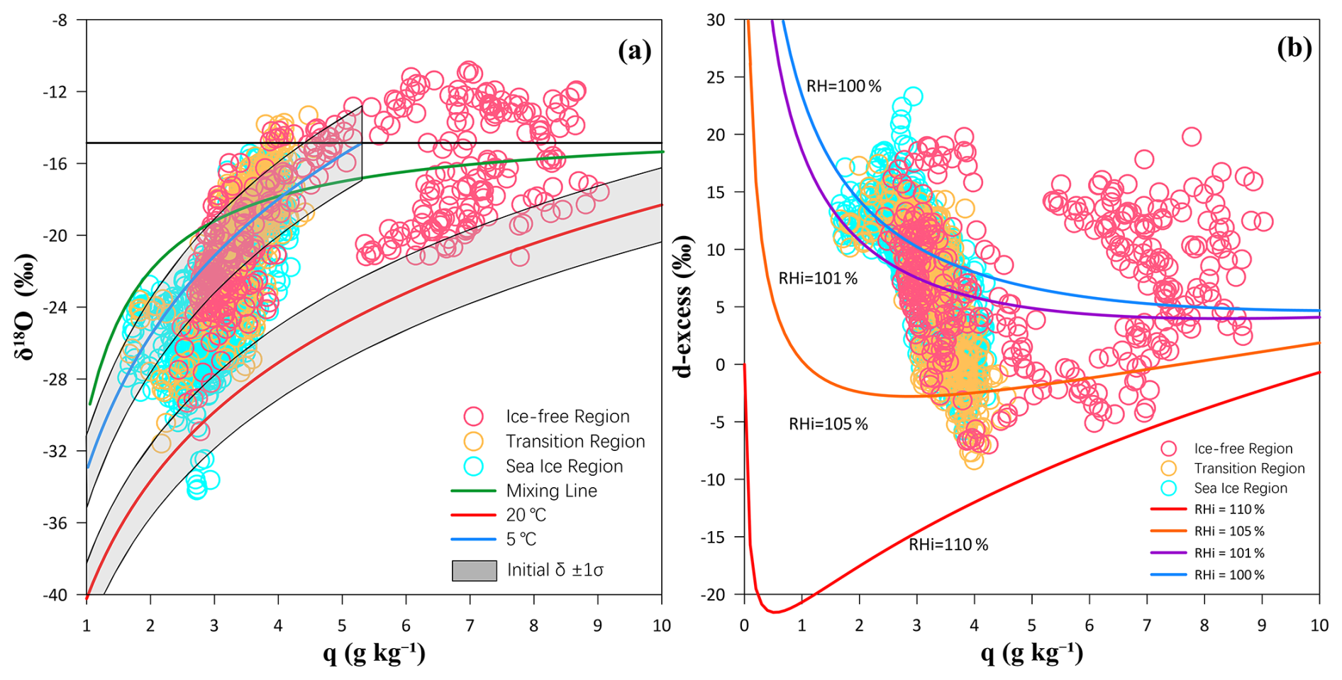
Figure 6 Water vapor δ¹⁸O (a) and d-excess (b) versus specific humidity (q). Data points are color-coded by sea ice regime, theoretical Rayleigh distillation curves and mixing/supersaturation curves are shown as colored lines (see legends). In panel (a), Rayleigh curves were initialized using isotopic compositions representative of mid-latitude conditions (40–60° N; $\mathit{\delta }{}^{\mathrm{18}}\mathrm{O}=-\mathrm{14.86}$ ‰). Shaded areas indicate the range of theoretical Rayleigh curves associated with ±1 standard deviation variations in the initial δ¹⁸O values. Initial specific humidity was calculated assuming saturation at the corresponding source temperature (q₀=14.3 and 5.31 g kg⁻¹). In panel (b), colored curves represent supersaturation scenarios initialized with d-excess=5.01 ‰ under the same fixed initial specific humidity (q₀=14.3 g kg⁻¹).

In the Sea Ice and Transition Regions, q–δ¹⁸O observations cluster near or between the 5 and 20 °C Rayleigh curves (Fig. 6a), consistent with vapor originating from advection and progressive dehydration during long-range transport. The q–d-excess relationship in these regions located around the Rayleigh curve (Fig. 6b), supporting the interpretation that Rayleigh distillation, rather than local kinetic fractionation, primarily governs water vapor isotopic variation in these regions. This also explains the contrasting temperature correlations observed in Fig. 4: a positive correlation for δ¹⁸O but a negative one for d-excess, reflecting the advection of warm, humid air from lower-latitude oceanic regions toward the Arctic.

However, the decline in dexcess is steeper than predicted by the equilibrium Rayleigh curve, with many points falling below it (Fig. 6b). This deviation indicates additional kinetic fractionation, most likely from cloud formation under icesupersaturated conditions, where the higher diffusivity of HDO compared to ${{\mathrm{H}}_{\mathrm{2}}}^{\mathrm{16}}\mathrm{O}$ leads to stronger fractionation of deuterium, suppressing dexcess in surrounding vapour (Clark and Fritz, 2013; Jouzel and Merlivat, 1984). Our calculations show that RH with respect to ice (RH_i) exceeding 105 % – common in polar regions – can reduce dexcess by over 10 ‰. This supersaturation-induced decline in water vapor d-excess has also been observed during dew deposition (Thurnherr and Aemisegger, 2022), indicating that supersaturated conditions drive d-excess reduction regardless of the phase transition pathway. Conversely, a limited number of points above the Rayleigh curve likely reflect contributions from sublimation of snow or sea ice (Kopec et al., 2019). Overall, the isotopic composition of water vapor in the Sea Ice and Transition Regions is primarily governed by Rayleigh fractionation during advective transport, while d-excess provides a distinct, sensitive record of local kinetic processes at the ice-atmosphere interface, such as supersaturation and sublimation. However, our interpretation of d-excess variations over sea ice is largely dependent on Rayleigh fractionation curves, with contributions from sublimation and processes under supersaturated conditions remaining poorly constrained.

In contrast, the Ice-free Region shows clear deviations from the theoretical Rayleigh distillation curves. Observations show a broad scatter in both q–δ¹⁸O and q–d-excess diagrams, indicating the interplay between advected and locally evaporated vapor under ice-free conditions. At lower specific humidity (<5 g kg⁻¹), isotopic patterns resemble those of ice-covered regions (Fig. 6), suggesting a persistent influence of advective moisture. However, as humidity rises (>5 g kg⁻¹) – which coincides with surface air temperatures exceeding ∼5 °C – systematic deviations from Rayleigh behavior become evident, reflecting an increased influence of local processes. In the q–δ¹⁸O diagram, two distinct patterns emerge: one cluster is enriched well above the mean mid-latitude δ¹⁸O value, indicating input from warm, isotopically heavy sources; the other falls below the 5 °C Rayleigh curve, where its scattered, non-logarithmic distribution – though still bounded by the 20 °C curve and the mixing line – points to strong kinetic fractionation. This divergence is systematically mirrored in the q–d-excess diagram (Fig. 6b), where values split both below and above the equilibrium curve. The co-occurrence of δ¹⁸O enrichment and elevated d-excess in this high-humidity regime supports the interpretation that kinetic fractionation during local evaporation as an important driver of Arctic water vapor isotopic composition under ice-free conditions.

In summary, Arctic water vapor isotopes exhibited contrasting characteristics between ice-covered and ice-free regions. In the Sea Ice and Transition Regions, isotope variations were broadly consistent with Rayleigh distillation during long-range water vapor transport, with possible modulation by kinetic effects associated with ice-related processes such as supersaturation and sublimation. In the Ice-free Region, however, the observed isotopic behavior deviated from the classical Rayleigh framework, reflecting enhanced influence of local evaporation and mixing with advected moisture over open water. Together, these results suggest that Arctic water vapor isotopic variability differs across sea ice conditions.

3.4 Evaluating the Influence of Local Evaporation on Ice-free Region Water Vapor Isotopes

To test whether local evaporation can account for the observed deviations from Rayleigh behavior, particularly elevated d-excess under warm and humid conditions, we applied the MJ79 marine boundary-layer evaporation model (Merlivat and Jouzel, 1979; Bonne et al., 2019). The model was driven by observed surface temperature and relative humidity and accounts for both equilibrium fractionation, controlled by temperature, and kinetic fractionation, modulated by relative humidity. Following Bonne et al. (2019), we adopted kinetic fractionation factors representative of the rough-wind regime (>7 m s⁻¹) for all simulations.

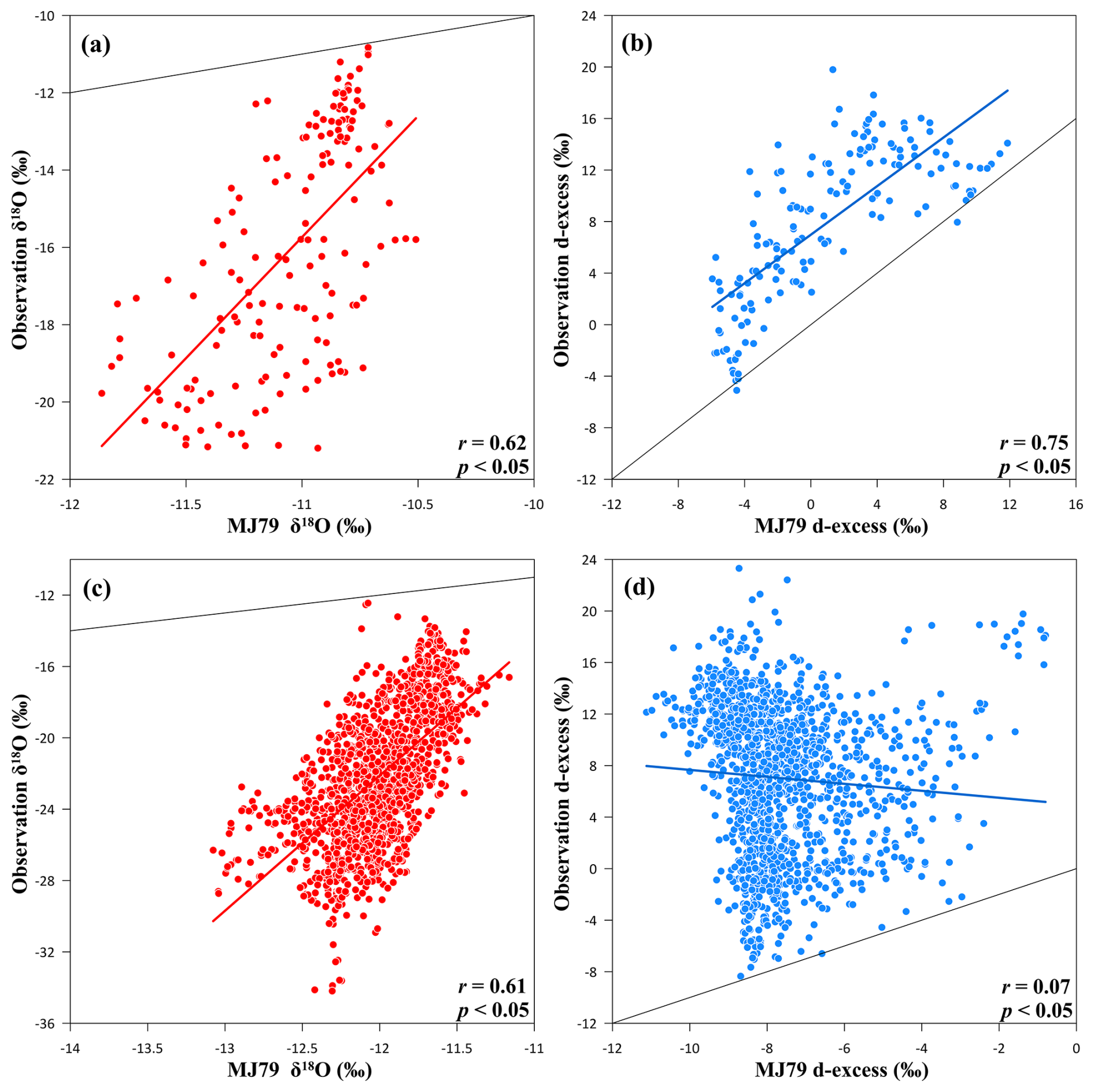
Figure 7 Observed versus MJ79-simulated water vapor isotopes (δ¹⁸O and d-excess) across sea ice regions under different temperature regimes: (a, b) >5 °C; (c, d) <5 °C. The black line denotes the 1:1 line (y=x).

First set of simulations were restricted to samples with temperatures exceeding 5 °C, corresponding to ice-free, high temperature-low relative humidity conditions where local evaporation is expected to dominate. Under these settings, the model reproduces the observed isotopic variability reasonably well, with correlations of 0.62 for δ¹⁸O and 0.75 for d-excess (Fig. 7a and b). This agreement supports the interpretation that kinetic fractionation during local evaporation contributes substantially to the isotopic composition of Arctic water vapor in the Ice-free Region. However, the model substantially overestimates the observed values, consistent with a previous study by Bonne et al. (2019). This overestimation largely reflects the closure assumption inherent in the MJ79 model, which treats local evaporation as the sole moisture source and neglects atmospheric mixing.

In contrast, when the temperature is below 5 °C, although the simulation shows a reasonable correlation with the observed δ¹⁸O (r=0.61), it fails to reproduce the d-excess variability (r=0.07) (Fig. 7c and d). This failure of the model to represent d-excess variability suggests that, under cold conditions, the moisture budget is dominated by non-local sources rather than local evaporation. This further supports our interpretation that advective moisture transport dominates isotopic variations in ice-covered regions.

3.5 Moisture Source Attribution from Lagrangian Trajectory Analysis

To test our isotope-based interpretation of moisture sources, we computed backward trajectories along the cruise track using the HYSPLIT model (Figs. 8 and S2–S4 in the Supplement). The analysis reveals a clear dichotomy in air mass origins aligned with sea ice regime. In the Sea Ice and Transition Regions, trajectories show air masses undergoing rapid cooling and dehydration during poleward transport, as reflected by declining specific humidity and rising relative humidity. Under these cold, saturated conditions, evaporation is suppressed, allowing Rayleigh distillation of advected moisture to emerge as the characteristic process, consistent with the observed alignment to Rayleigh curves (Fig. 6). Moreover, the frequent recirculation within the Arctic interior points to prolonged moisture residence under stable, cold conditions. This extended residency favors non-equilibrium ice-related processes, such as crystal formation and dew deposition under supersaturated conditions and sublimation, providing a coherent explanation for the distinctive d-excess signals observed in these regions (Fig. 6b).

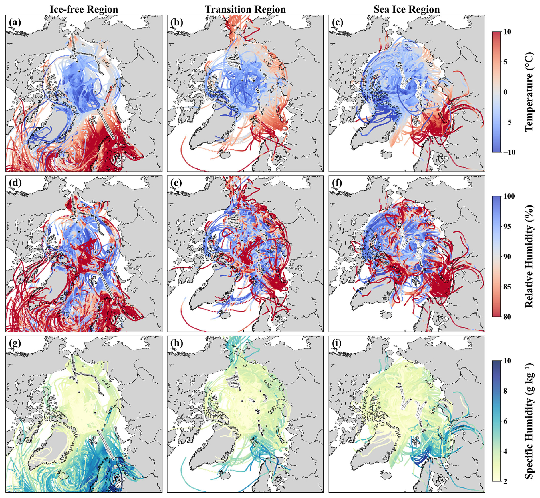
Figure 8 Ten-day HYSPLIT back trajectories from 10 m and associated meteorology by sea ice regime: ice-free (left), transition (middle), and sea ice (right). Rows show (a–c) air temperature (°C), (d–f) relative humidity (%), and (g–i) specific humidity (g kg⁻¹). Black stars denote start points.

In the Ice-free Region, however, trajectories reveal two distinct source pathways, explaining its complex isotopic signals. Most originate from lower latitudes, carrying warm, air northward across the Barents Sea. Elevated temperatures in the Barents Sea create a large saturation vapor deficit (via the Clausius–Clapeyron relationship), which maintains low relative humidity despite high specific humidity. These conditions promote strong evaporation over the ice-free ocean, contributing to the d-excess enrichment and reversed d-temperature relationship observed in this region (Fig. 4) and confirming that local evaporation is a major driver of isotopic variability under ice-free conditions. A smaller subset of air masses recirculates within the cold, saturated Arctic interior. Their limited interaction with open water suppresses evaporation, preserving an advective signature similar to that of ice-covered regions. Together, these dual air mass origins – one characterized by strong local evaporation and the other by advected moisture – explain the coexistence of both isotopic end-members observed in the q–δ¹⁸O and q–d-excess relationships.

3.6 Relative Contributions of Moisture Sources Across Arctic Sea Ice Regimes

To quantify the relative contributions of locally evaporated and advected moisture to Arctic boundary layer water vapor across different sea ice regimes, we apply the Bayesian isotope mixing model MixSIAR (Stock et al., 2018) to δ¹⁸O and δD measurements. Locally evaporated moisture is derived from Arctic open-water evaporation, with δ¹⁸O = −11.77 ± 0.59 ‰ and δD = −96.0 ± 7.7 ‰, estimated using the MJ79 model (see Sect. 2). Advected lower-latitude moisture, as identified by HYSPLIT trajectories (Fig. 8), primarily originates from the North Atlantic and the North Pacific, with isotopic endmembers taken from Benetti et al. (2017) near 50–60° N for the Atlantic (δ¹⁸O = −18.25 ± 4.79 ‰, δD = −138.5 ± 34.8 ‰) and from our observations over 50–60° N for the Pacific (δ¹⁸O = −15.54 ± 1.67 ‰, δD = −118.9 ± 9.0 ‰). A weighted average based on trajectory specific humidity (Atlantic = 79.07 % and Pacific = 20.93 %; see Sect. 2) is used to represent a single lower-latitude source (δ¹⁸O = −17.68 ± 3.8 ‰, δD = −134.4 ± 27.5 ‰). Calibrated vapor isotope measurements from each sea ice regime serve as the mixture input. A process error structure is applied to account for spatial variability and source uncertainty (see Sect. 2), and MixSIAR is run independently for each regime to estimate the probability distributions of source contributions.

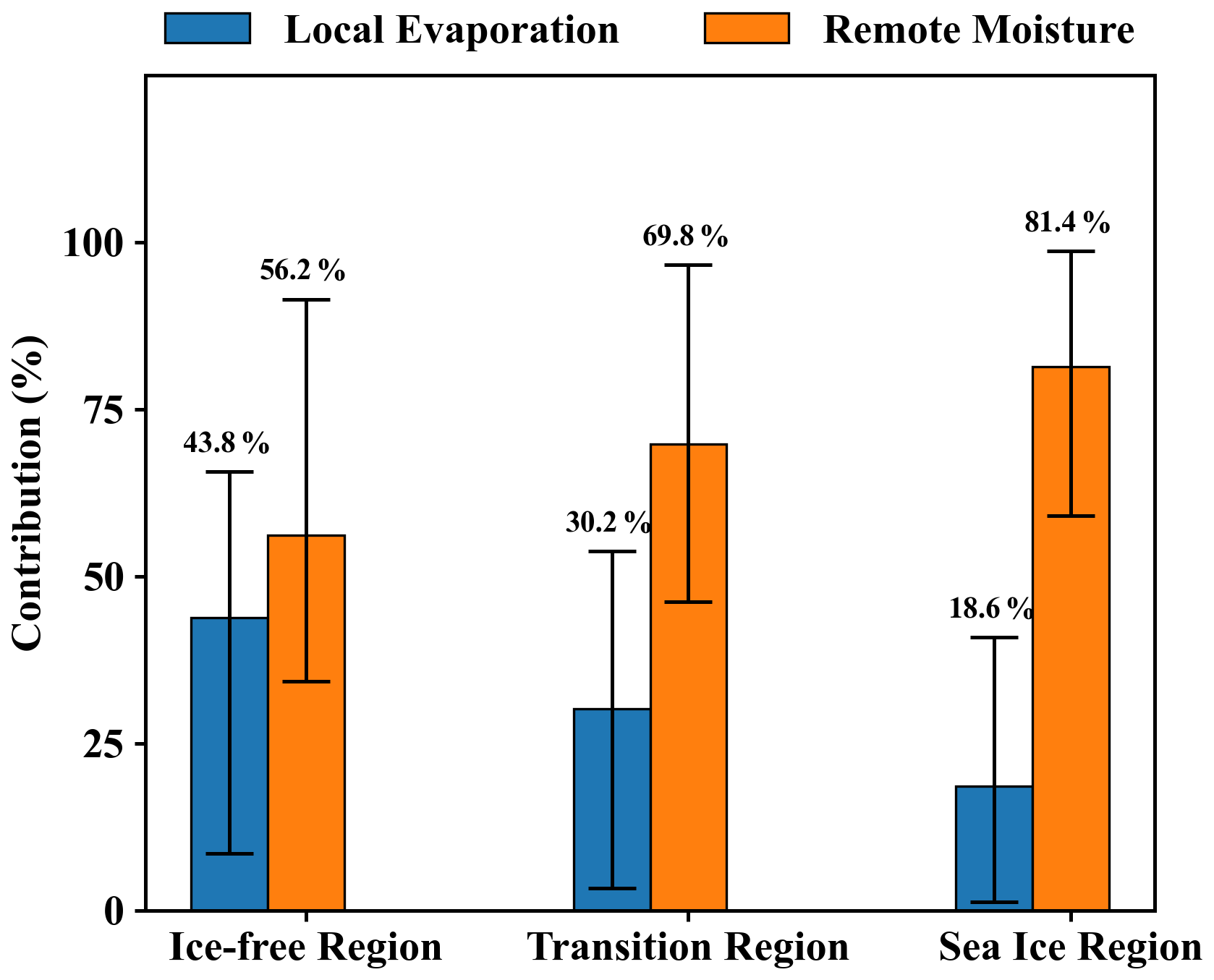
Figure 9 Contributions of local and low-latitude remote moisture estimated using a Bayesian isotope mixing model. Blue and orange bars indicate the proportions of local and low-latitude sources, respectively. Error bars denote the 95 % credible intervals (2.5 %–97.5 %), and the values above each bar represent the mean contributions.

MixSIAR results reveal a clear spatial gradient in moisture source contributions across sea ice regimes (Fig. 9). Local evaporation contributes most in the Ice-free Region, with a mean of 43.8 % (95 % CI: 14.7 %–65.7 %), decreasing to 30.2 % (95 % CI: 13.8 %–53.8 %) in the Transition Region and 18.6 % (95 % CI: 11.1 %–40.9 %) in the Sea Ice Region. Although the absolute contribution of local evaporation is modest, it increases progressively with decreasing sea ice cover. Across all regimes, advected lower-latitude moisture remains the dominant source, accounting for 56.2 %–81.4 % of boundary-layer vapor.

Sensitivity analyses further indicate that these source attribution results are not sensitive to reasonable variations in endmember definitions or prior assumptions (Figs. S5 and S6). These findings indicate that, while long-range transport governs the Arctic vapor budget, local evaporation contributes a notable fraction in ice-free areas.

4 Discussion and Conclusions

4.1 Water Vapor Isotopic Responses to Distinct Sea Ice Regimes

Our sea-ice-based isotope framework helps reconcile previously conflicting interpretations of Arctic vapor d-excess by showing that, although dexcess has traditionally been treated predominantly as a source signature (Dansgaard, 1964), it is also highly sensitive to humidity and local evaporation conditions associated with different sea-ice regimes. Since the first polar vapor isotope measurements reported unexpectedly higher dexcess in Arctic-sourced moisture compared with lower latitudes (Kurita, 2011), subsequent studies have alternately documented both high (Kopec et al., 2019) and low (Klein et al., 2015; Brunello et al., 2023) values under similar surface conditions. These apparently conflicting results likely reflect sampling under contrasting sea-ice and humidity conditions associated with different kinetic fractionation environments, rather than intrinsic differences in moisture sources.

Previous studies have reported conflicting relationships between polar vapor d-excess and sea ice. Bonne et al. (2019) found a positive correlation with sea ice, whereas Klein and Welker (2016) reported a negative correlation. This divergence likely stems from differences in the study domain, which sample distinct sea-ice regimes. Bonne et al. (2019) primarily analyzed regions with sea-ice coverage greater than zero, corresponding to the transition-to-ice-covered regime in our study, where d-excess increase with SIC (Fig. S1a). In contrast, Klein and Welker (2016) focused largely on the low-ice Bering Strait, an environment analogous to our ice-free-to-transition region, in which the negative correlation reflects enhanced local evaporation over open water (Fig. S1b). By spanning multiple sea-ice regimes, our observations during the cruise period reveal that d-excess does not exhibit a simple monotonic relationship with sea ice, but instead shows a bimodal distribution, with elevated values in both ice-covered and ice-free regions. This pattern reflects contrasting controlling mechanisms between the two regimes: the ice-covered region is dominated by long-distance Rayleigh fractionation superimposed by sublimation, whereas the ice-free region is governed primarily by local evaporation dynamics.

Our analyses are based on a classification of observations into sea-ice regimes, which provides an analytical framework for organizing the data. While these regime-dependent differences highlight distinct isotopic behaviors, the sea-ice-based classification should be viewed as an analytical framework rather than a strict representation of discrete physical boundaries. Some overlap between categories, particularly between the transition and ice-covered regimes, is therefore expected due to the continuous nature of environmental variability along the cruise track. Results should thus be interpreted in terms of environmental gradients rather than strictly separated regimes. Future studies could further explore isotope variability using continuous variables such as SST and humidity to complement this regime-based perspective.

4.2 Relationship between isotopes and local meteorological conditions

A negative d-excess–RH relationship is widely observed at both regional (Uemura et al., 2008) and global scales (Pfahl and Sodemann, 2014). In the Arctic, however, the relationship remains poorly constrained due to the paucity of isotopic measurements. Our cross-Arctic water vapor isotope observations reveal an overall negative relationship between d-excess and RH, but with a progressively weaker correlation from the ice-free region to the sea-ice-covered region, indicating a diminishing influence of local evaporation as sea ice increases (Fig. 5). The slopes of the d-excess–RH relationship range from −0.46 ‰ to −0.26 ‰ across the different Arctic regimes and are comparable to values reported at lower latitudes (e.g., −0.4 ‰; Thurnherr et al., 2020), highlighting the important role of local evaporation in shaping near-surface water-vapor d-excess. However, it should be noted that RH in this study is derived from in situ air temperature rather than SST, which may partly weaken the correlations and affect the estimated slopes. Nevertheless, because air temperature and SST co-vary closely over the Arctic (Klein and Welker, 2016), the inter-regional contrasts in the d-excess–RH relationship identified here remain valid.

In contrast, our observations reveal pronounced differences in isotope–temperature relationships between the ice-free and ice-covered regions. The δ¹⁸O–temperature correlation weakens from the ice-covered region toward the ice-free region and becomes clearly negative when temperatures exceed 5 °C in the ice-free region (Fig. 4a). This interpretation is further supported by the d-excess–temperature relationships, which show weak correlation in the ice-free region but strong one in the ice-covered region (Fig. 4b). These patterns are consistent with previous observations over open water (Bonne et al., 2019; Klein and Welker, 2016; Sodemann et al., 2024) and in the ice-covered region (Brunello et al., 2023, 2024), respectively. However, Brunello et al. (2024) and Sodemann et al. (2024) attributed the positive δ¹⁸O-temperature and negative d-excess–temperature relationships to warm air intrusions, based on observed positive RH–temperature coupling. By contrast, our observations show a clear negative correlation between RH and temperature, indicating that the observed isotope variability is more consistent with local processes under contrasting sea-ice conditions rather than synoptic-scale moisture advection (Fig. 3). This difference likely reflects the contrasting observational frameworks, with our short-duration transect sampling being less sensitive to episodic warm-air intrusions.

4.3 Quantifying the Shift in Moisture Sources

Stable water isotopes provide a quantitative framework to partition moisture source contributions across the study domain. The contribution from local evaporation increases from 18.6 % in the Sea Ice Region to 43.8 % in the Ice-free Region, demonstrating enhanced local recycling despite persistent advective dominance. This gradient aligns with observed surface moisture flux trends (Boisvert and Stroeve, 2015) and contextualizes previous observationally or model-based estimates ranging from 8 % (Domínguez et al., 2018) to over 35 % (Zhong et al., 2018). By providing a novel quantification based on vapor isotopes, this study highlights the capacity of in-situ isotopic monitoring to resolve complex Arctic hydrological processes.

Although we quantify the relative contributions of remotely advected and local evaporated moistures across different ice regimes, there are at least two caveats that should be noted. First, uncertainties arise from the determination of the end-members. In particular, the remote end-member is constrained by limited low-latitude sampling and by the use of boundary humidity rather than a full Lagrangian moisture budget, which may bias the estimated contribution of remote sources by neglecting moisture turnover along transport pathways. In addition, although the MJ79 model serves as a standard local-evaporation end-member, its closure assumption neglects atmospheric mixing and synoptic processes (Bonne et al., 2019). Consequently, the simulated isotopic composition should be interpreted as a theoretical local-evaporation end-member rather than an exact representation of atmospheric conditions. Second, the Bayesian mixing model relies on the combined use of δ¹⁸O and δD, which are strongly correlated. This high correlation reduces the effective dimensionality of the isotopic constraints, limiting the ability of the model to robustly distinguish between the two end members and introducing additional uncertainty. Despite these caveats, our results suggest that enhanced local moisture contributions are associated with reduced sea-ice conditions, consistent with the hypothesized feedback whereby sea-ice retreat promotes a more localized Arctic water cycle, as recorded in both water-vapor (Bailey et al., 2021) and precipitation (Kopec et al., 2016) isotopes. These results provide in-situ isotopic observational constraints for evaluating near-surface humidity, precipitation recycling, and the fidelity of regional climate models.

4.4 Implications for Arctic Hydroclimate Research

Beyond contemporary implications, our findings necessitate refinements in paleoclimate interpretations from polar ice-core records. The canonical δ¹⁸O–temperature relationship, long used as a paleo-thermometer, is modulated by sea ice extent: under extensive ice cover, strong positive correlations reflect temperature-driven advective distillation, whereas in Transition and Ice-free Regions, the relationship weakens or reverses, indicating that δ¹⁸O integrates local evaporation and humidity signals alongside temperature. Enriched δ¹⁸O with elevated d-excess during warm, ice-reduced periods (e.g., interglacial) reflects reorganized local moisture sources rather than temperature alone. We therefore advocate interpreting δ¹⁸O–d-excess co-variation within the context of different sea-ice regimes to help disentangle past temperature and sea ice signals, thereby linking modern process understanding with paleo-isotope interpretation.

While our study proposes a sea ice–mediated isotopic framework, several research frontiers warrant further investigation. Extending observations across seasons and years could help assess the climatological robustness of the proposed framework, while expanding spatial coverage and incorporating additional tracers (e.g., ¹⁷O-excess) may provide further constraints on the underlying mechanisms. Integrating this framework with isotope-enabled climate models could facilitate evaluation of model performance across both past and projected climates, while applications to ice-core records may offer additional insights into the relative influences of temperature and sea-ice variability. Collectively, these efforts could advance our understanding of Arctic isotope processes and hydroclimate responses under ongoing climate change.

In summary, this study demonstrates that Arctic near-surface water vapor isotopes exhibit contrasting characteristics between ice-covered and ice-free conditions, reflecting differences in moisture sources and fractionation processes. Under extensive ice, advective Rayleigh distillation dominates, producing a strong δ¹⁸O–temperature correlation and elevated d-excess in colder regions. As sea ice retreats, local evaporation over open water contributes more, imprinting a kinetic fingerprint of enriched δ¹⁸O and elevated d-excess under warm, dry conditions. This shift breaks down the canonical δ¹⁸O–temperature relationship, giving rise to an “anti-temperature” effect. Quantifying this regime shift, our Bayesian mixing model constrained by in-situ isotopes reveals that local evaporation contributions rise from 18.6 % in the Sea Ice Region to 43.8 % in the Ice-free Region – demonstrating a 2.4-fold enhancement of local recycling despite persistent advective dominance. These results highlight the important influence of contrasting sea-ice conditions on Arctic isotopic variability across the ice–open water transition, and provide observational constraints for both contemporary hydroclimate variability and paleoclimate interpretation.