Exploring atmospheric CH₄ monitoring network expansion in Italy using inverse modelling

Top-down approaches using inverse modelling provide valuable complementary information to national methane emission inventories, which are primarily based on bottom-up methods. Here, we focus on Italy, where methane is currently monitored at five stations that belong to the Integrated Carbon Observation System (ICOS). Top-down estimates show substantial discrepancies over this country, suggesting that the current network provides weak observational constraints on methane fluxes. In this study, we assess the potential expansion of Italy's ICOS network using Observation System Simulation Experiments (OSSEs) and inverse modelling. Eight candidate sites were identified, selected either from existing non-ICOS monitoring stations or from proposed future locations. To conduct the OSSEs, we use the ICON-ART model coupled with the Community Inversion Framework (CIF). We design a set of network expansion scenarios to evaluate the potential of each candidate station to improve emission constraints and include four additional scenarios to quantify the contribution of existing and idealized networks. To reduce the influence of randomness, multiple emission scenarios are constructed. Among all candidates, Chieti (CHI; 42.2° N, 14.7° E) and Mount Venda (VND; 45.3° N, 11.7° E) emerge as the most effective additions, with Chieti showing a slight overall advantage. Chieti enhances constraints mainly in Central and Southern Italy, while Mount Venda is particularly effective in Northern Italy, where most anthropogenic methane emissions originate. The framework developed here can be readily applied to other countries aiming to optimize their atmospheric measurement networks and to improve constraints on greenhouse gas emissions.

1 Introduction

The Paris Agreement (PA) under the United Nations Framework Convention on Climate Change (UNFCCC) commits nations to limit global temperature rise to below 2 °C compared to pre-industrial levels (UNFCCC, 2015). Countries that are parties to the UNFCCC must report their greenhouse gas (GHG) emissions, fostering transparency, tracking progress, and promoting international cooperation on climate change. Currently, countries primarily report their emissions through bottom-up inventories, which typically rely on (1) socioeconomic and environmental data, (2) source-specific emission factors, and, for some sectors such as Land Use, Land Use Change and Forestry (LULUCF), (3) process-based models. However, compiling these inventories is resource-intensive, time-consuming, and typically completed with a 2-year delay. The quality of reporting also varies significantly between nations due to differences in resources and technical capabilities. To support the PA's mitigation goals, top-down monitoring systems can complement bottom-up inventories, as recognized by the 2019 Refinement to the 2006 IPCC Guidelines for National Greenhouse Gas Inventories (Calvo Buendia et al., 2019).

Top-down methods, also known as inverse modeling, rely on atmospheric transport models and data assimilation techniques. By assimilating observed atmospheric GHG concentrations through statistical approaches (e.g., Bayesian frameworks), these methods can help reconcile bottom-up inventories (prior estimates) with atmospheric observations, resulting in refined posterior estimates of emissions. Top-down methods provide independent estimates that are comparable across regions and over time, are available more quickly than bottom-up estimates, and can be produced at global, regional, national, and sub-national scales (Janssens-Maenhout et al., 2020; Bergamaschi et al., 2018). However, the quality of these top-down estimates heavily relies on the coverage and the precision of atmospheric measurements. Observational in-situ networks should therefore be carefully designed to minimize the uncertainties of existing bottom-up inventories and improve our ability to track the temporal evolution of GHG fluxes at regional and national scales.

To address the needs for better measuring the atmospheric GHG concentrations as well as the fluxes between the atmosphere, the land surface and the oceans, the European Union has created the Integrated Carbon Observation System (ICOS; Heiskanen et al., 2022). It is an observational network that provides data from about 180 measurement stations of three different types, Atmosphere, Ecosystem, and Ocean, across 16 European countries. Since its establishment in the early 2010's, ICOS has been continuously expanding its observation network. Today, the Atmosphere network consists of 48 stations (40 labeled and 8 candidate stations) measuring GHG atmospheric concentrations across Europe. In the inversion community, ICOS data are widely relied upon for several key reasons:

• Instrumentation is harmonized across sites

• Measurements are calibrated against a common reference scale

• Measurements follow strict protocols for calibration, sampling, and data processing

• Data undergo both automated and expert quality control

• Data are open-access and provided in standardized formats

• Data are typically accessible with a delay of approximately one day for near-real-time products (ICOS RI, 2018), whereas quality-checked fast-track data releases become available after a delay of a few months (ICOS RI et al., 2026).

Together, these features ensure direct comparability between observations, low observational uncertainties, long-term consistency, and easy access and integration into inversion systems, as opposed to data from stations that are not part of the ICOS network.

Among the well-mixed GHGs, anthropogenic methane (CH₄) has the second largest influence on global warming. This gas has a global warming potential approximately 80 times higher than carbon dioxide (CO₂) over a 20-year period (Forster et al., 2021) and also plays a crucial role in atmospheric chemistry, influencing ozone formation and hydroxyl radical (OH) concentrations. Hence, reducing CH₄ emissions can yield rapid climate and air pollution benefits, which emphasizes the need for accurate quantification of its sources and sinks (Saunois et al., 2025), and making it a key target for the climate mitigation efforts requested by the PA. Bottom-up estimates show that Italy is a significant CH₄ emitter in Europe, with major contributions from agriculture (enteric fermentation and manure management), waste management and energy (see Sect. 2.3.1 and Romano et al., 2024). Natural emissions are also high in this region, with a strong influence of emissions from geological sources and wetlands (see Sect. 2.3.1). Italy signed the Global Methane Pledge at the 26th Conference of the Parties (COP26) in November 2021, committing to voluntary actions aimed at achieving a collective reduction in global methane emissions of at least 30 % from 2020 levels by 2030. Based on Caputo et al. (2022), the largest reductions in CH₄ emissions in Italy are expected in the waste sector, driven by evolving waste legislation, improved waste management practices, and increased treatment of waste in mechanical–biological and composting plants, as well as in anaerobic digesters. The second-largest reductions are projected in the agricultural sector, primarily due to more sustainable manure management practices (particularly anaerobic digestion with biogas production) and a decline in cattle and swine populations. In contrast, only limited changes are currently anticipated for natural emissions. While wetland emissions (mainly located in southern regions) may respond to climate change (e.g., Koffi et al., 2020; Zhang et al., 2017), they represent a relatively small fraction of total methane emissions compared to other sources, such as geological emissions, which are not expected to significantly change in the next decades.

Complementing bottom-up estimates and tracking the evolution of emissions through inverse modelling requires an observational network in Italy that provides adequate coverage of the country. At present, five ICOS sites are monitoring continuously CH₄ in Italy: Plateau Rosa (PRS; 45.9° N, 7.7° E), Ispra (IPR; 45.8° N, 8.6° E), Potenza (POT; 40.6° N, 15.7° E), Monte Cimone (CMN; 44.2° N, 10.7° E) and Lampedusa (LMP; 35.5° N, 12.6° E). PRS and CMN have been measuring atmospheric CH₄ in Northern Italy since 2005 and 2008, respectively. These are mountain stations that primarily sample background air, with limited sensitivity to air mass pollution (Zazzeri et al., 2026) caused by transport processes such as advection, boundary layer growth, or thermally driven wind circulations (Fratticioli et al., 2023). These stations are therefore particularly valuable for constraining background concentrations, but they have limited sensitivity to regional emissions compared to continental lowland stations, such as POT. POT recently began monitoring CH₄ (Lapenna et al., 2025) and is expected to provide valuable coverage in Southern Italy in the future. However, it remains difficult to assess how well observations at this location can be reproduced by transport models. IPR has been measuring since 2017, but is located in a valley surrounded by complex terrain, making it challenging to simulate accurately. LMP is a marine remote site located on Lampedusa island, deep in the Mediterranean sea and distant from continental Italy, monitoring since 2008. While it provides useful information on background concentrations, its ability to constrain Italian emissions is inherently limited due to its distance from continental sources. These various limitations help explain why top-down estimates over Italy show substantial discrepancies (see e.g., Ioannidis et al., 2026) and motivate our focus on Italy to improve the observational network. Additional stations, introduced in Sect. 2.4, also monitor CH₄ in Italy. However, these sites are not part of the ICOS network. They do not comply with ICOS standards for measurement systems and quality assurance protocols, and their data are not available in near real time.

Here, we conduct Observation System Simulation Experiments (OSSEs) with the Eulerian model ICON-ART (Zängl et al., 2015; Hoshyaripour et al., 2026) to assess the effectiveness of the current ICOS monitoring network in Italy and evaluate potential expansions. This work complements a recent study that investigated the same expansion in Italy for CO₂ monitoring using Lagrangian modelling (Villalobos et al., 2025). Both studies are conducted within the framework of the EU-HORIZON Attributing and Verifying European and National Greenhouse Gas and Aerosol Emissions and Reconciliation with Statistical Bottom-up Estimates (AVENGERS) project. In the context of inverse modelling, OSSEs involve generating synthetic “true” emissions based on prior knowledge of their magnitude and associated uncertainties. These true emissions are then used to produce corresponding synthetic atmospheric observations using a transport model. We perform inversions by assimilating these synthetic observations representing the true atmospheric state to optimize the prior emission estimates. With each assimilated observation, the optimized emissions are expected to converge toward the true emissions. The degree of agreement between optimized and true emissions depends on the quality, spatial and temporal coverage, and quantity of observations in the network. OSSEs therefore provide a valuable framework to evaluate the impact of adding measurement sites, helping to identify optimal locations and compare different network expansion scenarios. OSSEs have previously been used in inverse modelling to assess the potential impact of existing or new surface stations (e.g., Takele Kenea et al., 2024; Park and Kim, 2020; Wang et al., 2018; Kaminski and Rayner, 2017; Wu et al., 2016; Hungershoefer et al., 2010; Baker et al., 2010) or satellites (e.g., Santaren et al., 2021; Yu et al., 2021; Basu et al., 2016; Bloom et al., 2016; Nickless et al., 2015; Ziehn et al., 2014; Shiga et al., 2014; Miyazaki et al., 2011; Villani et al., 2010; Edwards et al., 2009; Meirink et al., 2006; Rayner et al., 1996). In this work, alongside exploring the expansion of the Italian observational network, we build upon previous work and introduce a methodology that is both easily reproducible and adaptable to any country with Eulerian modelling. Furthermore, we employ the Community Inversion Framework (CIF; Berchet et al., 2021) to perform our inversions. Most of the Eulerian models used in the inversion community have now been coupled to CIF (LMDz, CHIMERE, ICON-ART, WRF, STILT, FLEXPART, TM5) and our methodology can therefore be easily applied with these models. This methodology also addresses an important caveat commonly found in the studies mentioned above: the impact of randomness and truth selection. Because the chosen truth is just one of many potential realities, the results can be artificially influenced toward a specific station when the prior and truth are already in good agreement around the station before the inversion. To mitigate such an effect, we adopt an ensemble of truth scenarios.

Section 2 introduces the transport model, inversion system, input data, and network scenarios considered in this study. It also outlines the generation of synthetic data and the choice of true emission data. Section 3 presents the results, while Sect. 4 addresses the caveats and limitations of the applied methodology.

2 Methods

Here, we describe the transport model, inversion framework, and input data used to generate the prior estimates, along with the network scenarios considered in this study.

2.1 ICON-ART model

The Icosahedral Nonhydrostatic (ICON) weather and climate model (Zängl et al., 2015) is a collaborative effort between the Deutscher Wetterdienst (DWD), the Max Planck Institute for Meteorology (MPI-M), the Deutsches Klimarechenzentrum (DKRZ), the Karlsruhe Institute of Technology (KIT), and the Center for Climate Systems Modeling (C2SM) in Switzerland. Its goal is to develop a unified, next-generation global system for numerical weather prediction (NWP) and climate modeling. ICON became operational within DWD's and MeteoSwiss' forecasting systems in 2015 and 2024, respectively. Notably, ICON was made available as open-source software to expand its user and developer community in February 2024. To incorporate atmospheric chemistry and aerosol processes, ICON is extended by the Aerosols and Reactive Trace gases (ART) module, developed and maintained by KIT (Hoshyaripour et al., 2026; Schröter et al., 2018; Rieger et al., 2015). This combination forms the ICON-ART model, a non-hydrostatic Eulerian chemical transport model that includes emissions, transport, gas-phase chemistry, and aerosol dynamics in both the troposphere and stratosphere. ICON-ART uses an icosahedral grid that can cover the entire globe or be restricted to limited areas, ranging in horizontal resolution from several degrees down to a few kilometers.

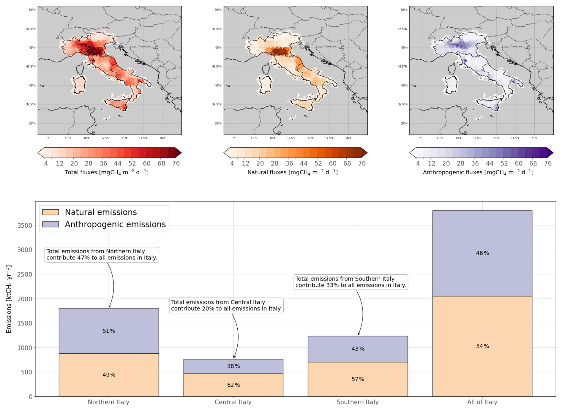
Figure 1 Spatial distribution of total, natural and anthropogenic fluxes in Italy (upper panels) and contributions of natural and anthropogenic emissions to total emissions in Northern, Central, Southern, and all of Italy (lower panel), based on the prior datasets. Numbers displayed at the center of bars represent the contribution of each category to the total emissions in a specific region.

For the present study, the model is configured with a horizontal resolution of 26 km (approximately 0.3°) over Italy and its surroundings (2–24° N, 32–54° E), consisting of 5048 grid cells (see Fig. 1, upper panels). Vertically, the model extends from the surface up to 23 km with 60 levels, using a height-based, terrain-following coordinate system.

Meteorological variables are computed online by the ICON model. In this setup, key prognostic variables (including wind speed, specific humidity, density, virtual potential temperature, and Exner pressure), are weakly nudged toward ERA5 reanalysis data (Hersbach et al., 2023, 2017) from the ECMWF, available at a 3-hourly temporal resolution. This nudging helps maintain the model's realism and prevents significant drift from observed atmospheric conditions. ERA5 data also provide the model's initial state. We simulate the year 2018 to be consistent with Villalobos et al. (2025).

Emission fields for transported species are processed via the Online Emissions Module (OEM; Jähn et al., 2020), integrated within ART. Output files of instantaneous concentrations are saved hourly and later interpolated in time, height, and space to derive model equivalents of observational data.

We do not consider atmospheric sinks as the air (along with emissions) is flushed out from our European domain in less than 20 d. We therefore neglect the effects of CH₄ oxidation in the atmosphere, as typically done in European inversions.

2.2 Community Inversion Framework

The Community Inversion Framework (CIF; Berchet et al., 2021) is an inversion system that has been designed to bring together the different inversion methods (analytical, variational and ensemble) and transport models used in the inversion community. It is built as an open-source, well documented, highly modular multi-model inversion framework written in Python that facilitates the comparison of (1) inversion methods and (2) transport models. CIF has proved to be accurate and computationally performant over the past years (Wittig et al., 2023; Savas et al., 2023; Remaud et al., 2022; Thanwerdas et al., 2024, 2022b, a)

We employ the ensemble square root filter (EnSRF) algorithm implemented in CIF to perform the inversions presented in this study. This algorithm has recently been improved and is thoroughly described in Thanwerdas et al. (2025). Briefly, an ensemble of vectors is used to represent the probability distribution of the control vector, which contains all the variables that we wish to optimize (e.g., fluxes, background concentrations, etc). Each member of the ensemble is attached to a different tracer transported by the model. After running simulations with this ensemble of tracers, the resulting ensemble of output concentrations is used to optimize the control vector to minimize the mismatch with the assimilated observations of atmospheric concentrations. In this study, the variables being optimized are scaling factors applied to the fluxes at the model's horizontal resolution.

The full assimilation time period is partitioned into several windows of finite length. For each window, a single scaling factor is associated with each optimized variable (e.g., flux emitted in a cell of the horizontal domain). Scaling factors within the window are optimized using both the observations from the current window and the observations from a fixed number (lag) of subsequent windows. Covariance localization is also applied to mitigate spurious long-range correlations that tend to appear in the ensemble. More details about the exact setup employed for this study is provided in Sect. 2.8.

2.3 Input data

The prior information is based on several high-quality datasets, which are merged into two categories of emissions: anthropogenic and natural. Total, anthropogenic and natural emissions are shown in Fig. 1 (upper panels).

2.3.1 Anthropogenic and natural fluxes

Except for fire emissions, all anthropogenic CH₄ fluxes are based on the TNO-AVENGERS inventory (van Mil et al., 2026). The TNO-AVENGERS inventory consist of national gridded inventories of Germany, Italy, the Netherlands, Sweden and Switzerland nested within the TNO-GHGco_v7 inventory for the other European countries. The approach to prepare the TNO-GHGco_v7 inventory is similar to CAMS-REG_v4 (Kuenen et al., 2022), but now also includes CH₄ emissions from the LULUCF sector. The yearly spatial distribution of emissions is provided at a horizontal resolution of 0.05° × 0.1° over Europe. Additionally, hour-of-day, day-of-week and month-of-year temporal scaling factors are also included in the dataset and were applied on the spatial distribution to create an hourly emission dataset. Fire emissions are based on the Global Fire Emissions Database version 4s (GFED4s; van der Werf et al., 2017) and are provided at a monthly resolution and a horizontal resolution of 0.25° × 0.25°.

According to these estimates of anthropogenic CH₄ fluxes, about 83 % of the anthropogenic CH₄ was emitted by the agriculture (mainly in Northern Italy) and waste sectors (spread over the country) in 2018 (see Fig. S1 in the Supplement). These sectors should therefore be the primary targets for improved anthropogenic emission constraints. The remaining emissions were mostly released by energy-related sources: fugitive sources (mainly in Northern Italy) and biofuel burning (spread over the country).

We use a dataset produced with the model LPJ-GUESS (Lund-Potsdam-Jena General Ecosystem Simulator, version 4.1, revision 12177; Smith et al., 2001) to represent the soil uptake and emissions from peatlands, inundated wetlands and mineral soils. LPJ-GUESS is a process-based dynamic vegetation-terrestrial ecosystem community model designed for regional or global studies of land surface processes. It has been developed by Lund University in a collaboration involving the Potsdam Institute for Climate Impact Research and the Max-Planck Institute for Biogeochemistry, Jena. This dataset is provided at daily temporal resolution and spatial resolution of 0.5°. For other natural sources, we rely on bottom-up estimates compiled for the inversions conducted as part of the Global Methane Budget (Saunois et al., 2020). These include the datasets for oceanic sources (including geological offshore and hydrate emissions), onshore geological sources and termites described in Saunois et al. (2020). These datasets are available at monthly temporal resolution and 0.1° × 0.1° spatial resolution.

According to these estimates, geological emissions largely dominate the prior natural emissions across all regions of Italy (ranging from 70 % in Southern Italy to 86 % in Central Italy), followed by emissions from wetlands (see Fig. S1).

Natural and anthropogenic datasets are resampled to hourly resolution, conservatively remapped to the ICON-ART spatial grid using the Emiproc package (Constantin et al., 2025) and aggregated to produce prior estimates of natural and anthropogenic emissions over Italy.

Monthly variations of emissions from anthropogenic and natural subcategories are displayed in Fig. S2. Among the natural emissions, only emissions from wetlands and uptake from mineral soils exhibit a sub-annual variability, which explains the seasonal cycle of the natural emissions. Among the anthropogenic emissions, the seasonal cycle is only driven by the energy-related emissions.

2.3.2 Background concentrations

Initial conditions and lateral boundary conditions for CH₄ mole fractions are derived from the CAMS global inversion-optimized CH₄ concentration product v21r1 (Segers et al., 2022). The data are based on surface observations only and are provided at a horizontal resolution of 3.0° × 2.0° and at a 6-hourly temporal resolution.

2.4 Candidate stations

For selecting candidate stations for the extended ICOS network, we consider 8 locations from Italy's existing or planned monitoring infrastructure:

• Mount Venda (VND, 45.3° N, 11.7° E). It is a proposed new site intended to improve constraints on emissions in the high-emission Po Valley region. A preliminary study investigated the possibility of installing a GHG sampling inlet at a transmission tower on the summit of Mount Venda (570 m), in the eastern Po Valley. However, this remains at the planning stage due to funding limitations.

• Chieti (CHI; 42.2° N, 14.7° E). This site has been recently established. It is operated by the University of Chieti and located on the Adriatic coast, and hast just begun measuring CH₄ in March 2026. At present, only “pilot” measurements are conducted, as calibrations are still not fully implemented and the World Meteorological Organization (WMO) compatibility goals are not achieved.

• Lecce (ECO; 40.3° N, 18.1° E). This site is located near the urban area of Lecce (population 94 377), about 10 km from the South Adriatic Sea. CH₄ measurements were continuously performed from 2015 to 2017 (Dinoi, 2025) by the National Research Council of Italy (CNR) – Institute for Atmospheric Science and Climate (ISAC). The station is active but GHG measurements are suspended.

• Lamezia Terme (LMT; 38.9° N, 16.2° E). This site is located along the Tyrrhenian Sea coastline, and CH₄ measurements have been conducted from 2015 to 2024 by CNR-ISAC (Malacaria et al., 2025). The CH₄ measurements are currently suspended due to flooding that affected the station.

• Capo Granitola (CGR; 37.6° N, 12.7° E). This site is located on the southern coast of Sicily facing the Strait of Sicily, and is jointly operated by CNR-ISAC and CNR-IAS (the Institute for the Study of Anthropic Impact and Sustainability in the Marine Environment). In situ CH₄ atmospheric observations were carried out here over the period 2015–2019 and 2022–2023 (Cristofanelli et al., 2025). The site remains active but GHG measurements are suspended.

• Madonie – Piano Battaglia (MDN; 37.9° N, 14.0° E). This site is located in a mountainous area in northern Sicily. Since 2005, ENEA (Italian National Agency for New Technologies, Energy and Sustainable Economic Development) has been performing weekly flask sampling (Sferlazzo et al., 2025).

• Monte Curcio (CUR; 39.3° N, 16.4° E). It is a mountain station located in the heart of the Calabria region, managed by the CNR-IIA (Institute of Atmospheric Pollution Research). Hourly CH₄ data are available from 2015 to 2017 (Bencardino, 2025). The station remains active but GHG measurements are suspended.

• Col Margherita (MRG; 46.8° N, 11.8° E). This observatory is located on the southern slope of the Eastern Alps, within the Dolomites. It is representative of the synoptic conditions of the south-facing Eastern Alps, where there is no similar station. The observatory is equipped with a complete meteorological station, an ozone analyser and a total gaseous mercury analyser, but the station does not monitor CH₄ concentrations.

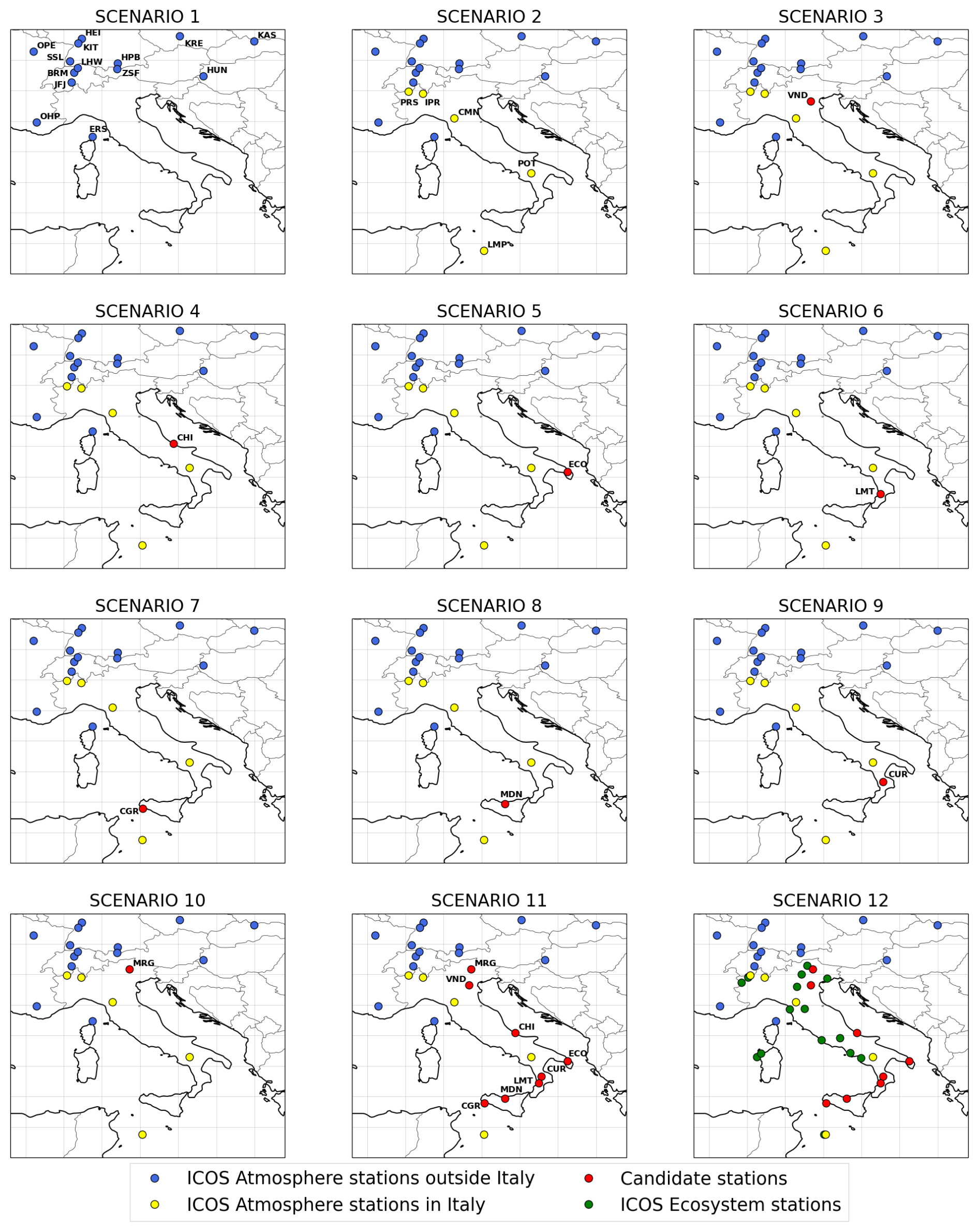
Figure 2 Description of the sites featured in the twelve atmospheric measurement network scenarios. The blue circles show the neighboring stations, i.e. outside Italy. The yellow circles show the ICOS Atmosphere sites in Italy. The red circles show the candidate stations studied in the scenarios 3 through 10. The green circles show the ecosystem ICOS stations. For readability, ICOS ecosystem station names are not displayed in Scenario 12, but are listed with their locations in Table A3.

ECO, LMT, CGR, CUR, MDN, and MRG are not part of ICOS but contribute to the regional Global Atmospheric Watch (GAW) programme of the WMO, which motivated their selection as candidate sites. Further information about these stations is provided in Table A1. Locations are displayed on a spatial map in Fig. 2 (e.g., Scenario 11). For stations already measuring CH₄, the ICOS label would require compliance with ICOS standards for measurement systems, quality-assurance protocols, as well as the adoption of a common data format for the near-real-time transmission of instrumental and diagnostic raw data to the ICOS Atmospheric Thematic Center (Hazan et al., 2016). Moreover, a sustained long-term commitment from national funding agencies is required to support the operational costs of the stations, as well as the national contributions required to ensure the operation of ICOS-labelled stations and their integration within the ICOS Research Infrastructure.

2.5 Network scenarios

This study evaluates twelve atmospheric measurement network scenarios encompassing Italy and its neighboring countries. The primary goal is to determine which candidate stations, introduced in Sect. 2.4, would provide the greatest benefit for constraining emissions in Italy. It results in eight different scenarios, each featuring one of the candidate stations. In addition, several supplementary network scenarios are considered to assess the contribution of existing networks and to estimate the optimal achievable constraints on Italian emissions. The twelve scenarios, displayed in Fig. 2, are outlined as follows:

• Scenario 1 includes only ICOS sites located in countries neighboring Italy. This configuration serves to assess the ability of external networks to constrain emissions originating within Italy.

• Scenario 2, referred to as the base network, expands on Scenario 1 by incorporating ICOS sites located within Italy.

• Scenarios 3 through 10 each evaluate the impact of adding a single additional station to the base network among the candidate stations. Specifically, the added stations are:

  • Scenario 3: VND

  • Scenario 4: CHI

  • Scenario 5: ECO

  • Scenario 6: LMT

  • Scenario 7: CGR

  • Scenario 8: MDN

  • Scenario 9: CUR

  • Scenario 10: MRG

• Scenario 11 combines the base network with all eight stations evaluated individually in Scenarios 3–10.

• Scenario 12 builds on Scenario 11 by further including all 16 Italian ICOS ecosystem stations, which are described in Table A3, to explore the potential of a dense measurement network in Italy.

These scenarios enable a systematic evaluation of how different network configurations influence the capacity to monitor and constrain GHG emissions across the region.

2.6 Characteristics of synthetic observations

Synthetic observations generated with the transport model ICON-ART are assimilated by the inversion system to refine prior estimates and to assess the potential of each candidate station for constraining emissions. Conducting robust OSSEs to identify the most suitable stations for network expansion requires producing synthetic observations with times and locations that closely replicate those of real-world measurements.

For existing stations, we use synthetic observations matching the locations and times of the real observations compiled in version 9.2 of the ICOS ObsPack CH₄ data product (ICOS RI et al., 2024). This dataset includes continuous measurements from 66 stations across Europe collected between 1984 and 2024, encompassing both ICOS and non-ICOS facilities. Within the temporal and spatial bounds of our experiments, data from 19 stations are available (blue and yellow circles in Fig. 2), with detailed station information provided in Table A2.

For both candidate and ecosystem stations, hourly measurements are assumed. To replicate the methodology of an inversion assimilating real data, only a subset of synthetic observations is used. At lowland sites, only the daily average of afternoon observations between 12:00 and 16:00 LT (local time) is assimilated to avoid challenges associated with simulating the boundary layer growth over the day. In contrast, at mountain sites, only the daily average of nighttime observations between 00:00 and 06:00 LT is assimilated, when these stations are more representative of background conditions and are less influenced by pollution transported by daytime upslope valley winds.

Regarding the required infrastructure, the main constraint was to remain consistent with the inlet heights assumed in Villalobos et al. (2025). In that study, a low inlet height of 2 m is used for mountain candidate sites, whereas a higher inlet height of 100 m is used for lowland candidate sites. Note that CHI is an exception, both here and in Villalobos et al. (2025), as it is a newly established station. At the start of this study, the projected inlet height was 50 m. We retained this value in our analysis because the installation of a substantially higher inlet in the coming years is considered unlikely.

The rationale behind the selection of 2 m and 100 m inlet heights is that model performance generally improves with increasing sampling altitude, provided that the surrounding terrain is not excessively complex and does not generate strong local flow disturbances. Higher sampling altitudes reduce the influence of very local processes, which require high spatial resolution to be accurately represented. Elevated sampling also increases the spatial footprint of the measurements, allowing observations to integrate signals from more distant source regions and thereby increasing sensitivity to large-scale flux patterns. However, sampling at excessively high altitudes, such as mountain stations located above the boundary layer, also has disadvantages. Air masses sampled at these altitudes are well mixed, making it more difficult to disentangle contributions from individual source regions. Consequently, such measurements are generally more effective at constraining background concentrations than regional emissions.

For lowland sites, a good sampling at existing ICOS sites is typically performed at around 100 m above ground level (see Table A2). This height helps reduce the influence of local processes, and obtain a good sensitivity to regional fluxes, while limiting costs and engineering challenges. At present, however, candidate stations that have previously measured CH₄ (ECO, LMT, CGR) sample below 100 m. Reaching such sampling heights would therefore require the installation of tall towers. Although this represents a substantial investment, implementation is expected to be more feasible at these locations because they already possess relevant infrastructure and experienced personnel conducting CH₄ measurements

For mountain sites, nighttime measurements are generally representative of the free troposphere, even when sampled close to the surface, owing to the elevated location of the stations. As a result, a sampling height of 2 m is sufficient, and this requirement is already met by existing mountain stations performing CH₄ measurements (MDN and CUR).

2.7 Generation of true emissions and synthetic observations

To generate synthetic observations with the ICON-ART transport model, we first sample a set of “true” scaling factors (representing the ratio of true to prior emissions) for each grid cell in the ICON-ART domain (c=5048 cells), following the approach described by Thanwerdas et al. (2025). We briefly present this approach here.

The true scaling factors are sampled from a normal distribution with a prior-error covariance matrix B. We account for both spatial and temporal correlations. For spatial correlations, we first construct a correlation matrix based on an exponential decay function, $e^{-\frac{d_{i,j}}{L}}$, where d_i,j denotes the great-circle distance between cells i and j, and L is the spatial correlation length. We then scale this matrix by the chosen variance to obtain the spatial covariance matrix. A similar procedure is applied to introduce temporal correlations, replacing spatial distances with the time interval between similar optimized variables (i.e., corresponding to the same cell), normalized by the temporal correlation length. The full covariance matrix, accounting for both spatial and temporal correlations, is built using Kronecker products. Using the singular value decomposition (SVD) of the full matrix B, we generate an ensemble of spatially and temporally correlated scaling factors. A major advantage of this approach is that it generates true fluxes consistent with the error statistics of the prior fluxes.

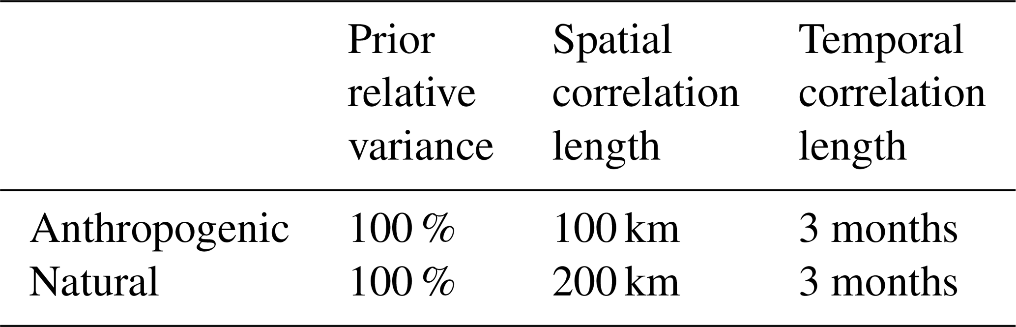
Distinct sets of true scaling factors are generated for anthropogenic and natural emission categories, and true total fluxes are computed as the sum of the true anthropogenic and natural fluxes. In line with the recommendations of Szénási et al. (2021) and anthropogenic correlation lengths estimated by TNO for Italy (Super et al., 2020), we adopt a spatial correlation length of 200 km for natural fluxes and 100 km for anthropogenic fluxes, considering no correlation for fossil fuel emissions and a correlation length of 150 km for agriculture and waste emissions. To determine the appropriate variance for each scaling factor, we compute the country-scale uncertainty for both flux categories using the specified correlation lengths and a range of relative variances (50 %, 100 %, 150 %, 200 %). Our analysis suggests that relative variances of approximately 150 % are required for both natural and anthropogenic fluxes to match the country-scale uncertainties reported by TNO (for anthropogenic fluxes) and by Szénási et al. (2021) (for both flux categories in Italy). However, applying relative variances above 100 % within a Gaussian framework increases the risk of generating negative flux values during the inversion. To balance realistic uncertainty representation with these technical constraints, we adopt a relative variance of 100 % for both flux categories. Although it results in a prior uncertainty that is slightly underestimated compared to existing estimates, it should not affect the conclusions of this study as we use an inversion set-up where true uncertainties are considered to be perfectly known. Note that, due to the shorter correlation length applied to anthropogenic fluxes, it results in a lower country-scale uncertainty for anthropogenic emissions compared to natural ones.

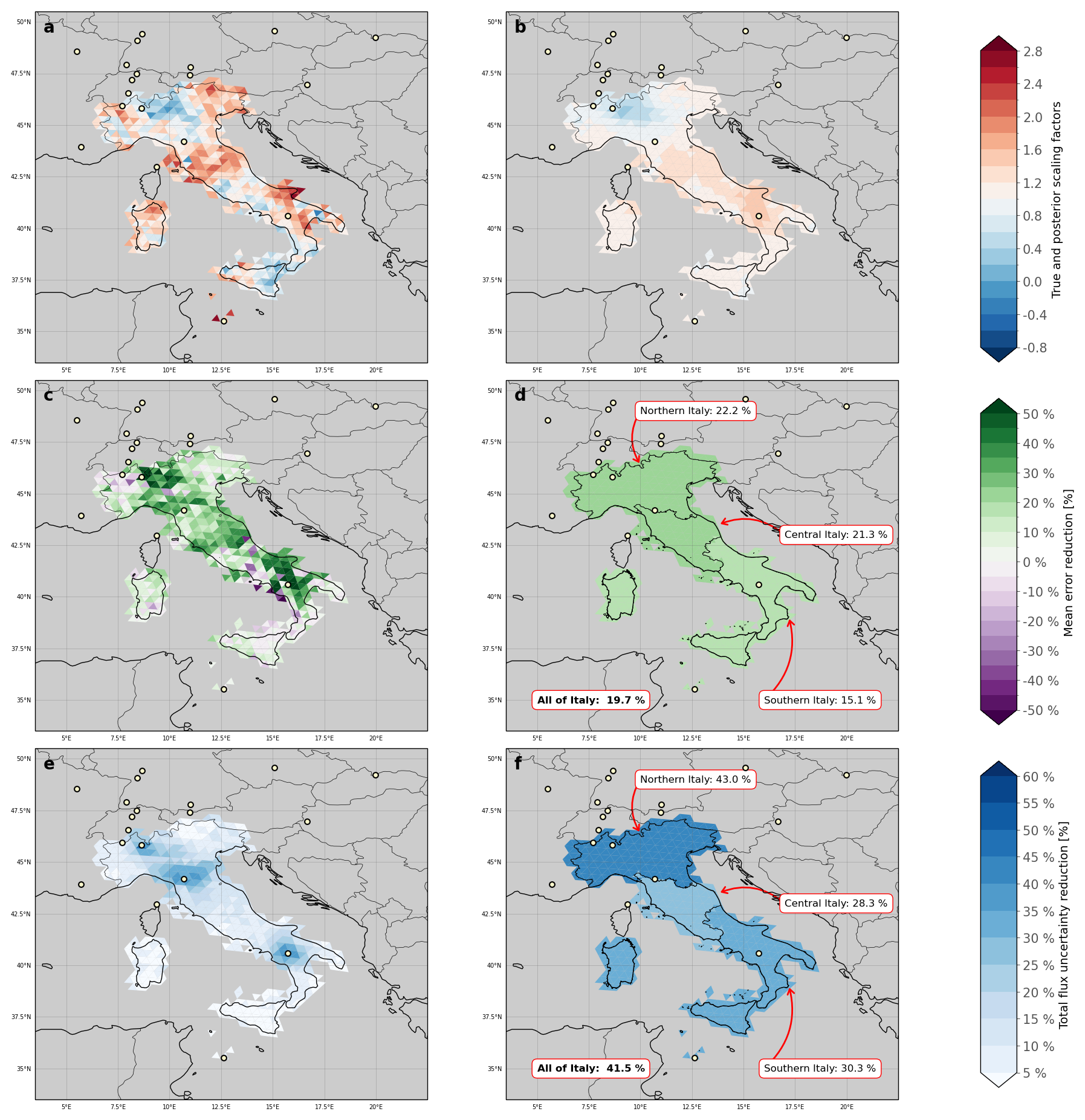
Figure 3 Illustration of the computation of the metrics presented in Sect. 2.9 for scenario 2, and for total CH₄ emissions. We first generate a set of true scaling factors (panel (a), averaged here over the full year). Among the five generated sets of true fluxes, we show only the fifth set here (orange circle in Fig. 5). The true scaling factors associated with the other truth scenarios are shown in Fig. S3. We start the inversion using prior scaling factors all equal to one. After the inversion, we obtain posterior scaling factors (b). Based on true, prior and posterior scaling factors, we compute ER (panel (c), averaged here over the full year) and annual MER for all Italian regions (d). We also compute UR (panel (e), averaged here over the full year) and annual TUR for the different Italian regions (f).

To account for a potential temporal variability of the mismatch between prior and true estimates, we generate a new set of true scaling factors for each 10 d period throughout the year 2018. To maintain seasonal coherence, we impose a temporal correlation using an exponential decay with a temporal correlation length of three months. An example of the resulting scaling factors, averaged over 2018, are shown in Fig. 3a. The perturbed fluxes used as the synthetic “truth” are obtained by applying these scaling factors to the corresponding prior fluxes. The selected values for prior relative variances and for spatial and temporal correlations lengths are summarized in Table 1.

Table 1 Selected values for prior relative variances and for spatial and temporal correlation lengths to build the prior-error covariance matrix B.

Finally, we run a 1-year forward simulation over 2018 with the perturbed fluxes. After this forward simulation, the simulated values matching the time and locations of the observations (for existing stations) or pseudo-observations (for candidate and ecosystem stations) introduced in Sect. 2.6 are stored. These simulated values are then treated as the new observations to be assimilated in the experiments presented in the next section. Additionally, to mimic realistic model-data mismatch uncertainties arising from both modelling and measurement errors, we perturb them with random values drawn from a Gaussian distribution with a mean of 0 and a standard deviation of 20 ppbv. This corresponds to the typical model-data mismatch calculated in Steiner et al. (2024b) with ICON-ART runs at a resolution of 26 km.

To cover a wider range of emission uncertainties, we replicate this methodology five times to generate five different sets of synthetic observations based on five different sets of true fluxes (hereinafter called truth scenario). The importance of using different truths for an OSSE is illustrated and discussed in Sect. 3.2.

Model–data mismatch plays a critical role in atmospheric inversions, as it directly affects the assimilation weights assigned to each observation and, consequently, the inversion outcomes. Assigning a uniform model–data mismatch across all stations implies equal trust in all observations. However, in real-data applications, model–data mismatch is inherently site-dependent. It reflects the degree of confidence in the model's ability to accurately simulate concentrations at a given location, which can vary due the model's ability to capture local atmospheric dynamics and local sources, given the complexity of the surrounding environment. In Sect. 3.5, we present a refined, station-specific estimation of model–data mismatch and analyze its impact on the inversion results. We chose to introduce results with a uniform model-data mismatch first, before incorporating the additional complexity associated with a realistic model-data mismatch. This choice serves several purposes in the initial phase of our study. First, it provides a consistent and fair basis for comparing candidate stations, which would not be possible with a realistic model-data mismatch that varies across locations. Second, there is no guarantee that the model-data mismatch estimated using our methodology will accurately reflect real conditions once a station becomes operational. In practice, experience shows that trying to predict how well a model will reproduce observations from a new station is highly challenging. Finally, it facilitates the interpretation of the results. Using a uniform model-data mismatch is not sufficient on its own, which is why we present results from both approaches.

2.8 Inversion setups

For each designed network and each set of true fluxes and perturbed observations, we run a 1-year inversion (i.e. 12 network scenarios × 5 truth scenarios = 60 inversions) spanning 2018 with the EnSRF mode of CIF-ICON-ART. Following the conclusions of Thanwerdas et al. (2025), we use the following CIF settings to run all the inversions:

• Window length = 10 d

• Number of lags = 2

• Localization function is an exponential function

• Localization length = 600 km

To build the prior error-covariance matrix B, relative variances and spatial and temporal correlations are prescribed to match the values used in generating the true scaling factors (see Table 1).

2.9 Evaluation metrics

We use two different metrics to quantitatively compare network designs: error reduction and uncertainty reduction. Here, we define these metrics.

2.9.1 Error reduction (ER)

The error reduction (ER) quantifies the agreement between the optimized fluxes and the true fluxes. It is defined by:

$$\begin{array}{}\text{(1)}& \begin{array}{rl}\mathrm{ER}(k,t)& =\mathrm{1}-{\displaystyle \frac{{\mathit{e}}_{\mathrm{a}}(k,t)}{{\mathit{e}}_{\mathrm{b}}(k,t)}}\\ & =\mathrm{1}-{\displaystyle \frac{\left|{\mathit{x}}_{\mathrm{a}}(k,t)\cdot \mathit{F}(k,t)-{\mathit{x}}_{\mathrm{t}}(k,t)\cdot \mathit{F}(k,t)\right|}{\left|{\mathit{x}}_{\mathrm{b}}(k,t)\cdot \mathit{F}(k,t)-{\mathit{x}}_{\mathrm{t}}(k,t)\cdot \mathit{F}(k,t)\right|}}\end{array}\end{array}$$

Here, x_b(⋅), x_a(⋅) and x_t(⋅) are the vectors representing the prior, posterior, and true scaling factors. In this work, F(⋅) is either the anthropogenic flux, the natural flux or the sum of them; e_b(⋅) and e_a(⋅) are the prior and posterior absolute flux errors, respectively. k and t represent the cells of the model's horizontal grid and the time dimension, respectively. This formula gives a quantity that is time dependent and spatially distributed. A positive ER indicates that the optimized fluxes agree better with the truth than the prior data, whereas a negative ER shows the opposite. We further define the mean error reduction (MER) using time and area-weighted spatial averages of the flux errors,

$$\begin{array}{}\text{(2)}& \begin{array}{rl}\mathrm{MER}(\mathcal{S},\mathcal{T})& =\mathrm{1}-{\displaystyle \frac{{\stackrel{\mathrm{‾}}{{\mathit{e}}_{\mathrm{a}}(k,t)}}^{\mathcal{S},\mathcal{T}}}{{\stackrel{\mathrm{‾}}{{\mathit{e}}_{\mathrm{b}}(k,t)}}^{\mathcal{S},\mathcal{T}}}}\\ & =\mathrm{1}-{\displaystyle \frac{{\sum }_{k\in \mathcal{S},t\in \mathcal{T}}\mathit{a}\left(k\right)\cdot {\mathit{e}}_{\mathrm{a}}(k,t)}{{\sum }_{k\in \mathcal{S},t\in \mathcal{T}}\mathit{a}\left(k\right)\cdot {\mathit{e}}_{\mathrm{b}}(k,t)}}\end{array}\end{array}$$

Here, 𝒮 and 𝒯 denote the spatial and temporal domains, respectively. 𝒮 may represent the spatial extent (the entire domain or a region in it), while 𝒯 refers to the temporal extent (the full year or a specific season). a(⋅) denotes the area of a given grid cell. In this study, we consider the entire country and three aggregated regions.

The aggregation is based on the five Eurostat Nomenclature of Territorial Units for Statistics (NUTS) regions of Italy: Northern-West, Northern-East, Central, Southern, and Insular Italy. For our analysis, we combine the two northern regions into a single Northern Italy and merge Insular Italy with Southern Italy, resulting in three regions of comparable area. This division of the entire domain facilitates the quantification of spatial heterogeneity of our results.

It is important to note that the MER does not reflect improvements in domain-total fluxes, as it is based on the sum of absolute errors rather than net differences. Reductions in domain-total flux error can be misleading, as they may result from compensating errors across spatial or temporal domains. For example, a positive error in Northern Italy (overestimation of emissions) and a negative error in Southern Italy (underestimation of emissions), if of equal magnitude, will result in an accurate estimate of emissions at the national scale. In contrast, a high MER reflects a consistent and widespread agreement between posterior and true fluxes, offering a more robust measure of overall inversion performance. MER can be calculated for different regions, seasons, and flux categories. Illustrative examples of ER and MER are provided in Fig. 3c and d, respectively.

2.9.2 Uncertainty reduction (UR)

For each cell of the horizontal domain, we define the uncertainty reduction (UR) as the reduction in the ratio of posterior to prior uncertainties,

$$\begin{array}{}\text{(3)}& \mathrm{UR}(k,t)=\mathrm{1}-{\displaystyle \frac{{\mathit{\sigma }}_{\mathrm{a}}(k,t)}{{\mathit{\sigma }}_{\mathrm{b}}(k,t)}}\end{array}$$

where σ_b(⋅) and σ_a(⋅) denote the vectors representing the prior and posterior standard deviations of scaling factors, respectively. We further define the total flux uncertainty reduction (TUR) as the uncertainty reduction of the domain-total flux (e.g., all of Italy or a specific region in Italy).

$$\begin{array}{}\text{(4)}& \begin{array}{rl}\mathrm{TUR}(\mathcal{S},\mathcal{T})=& \mathrm{1}-\sqrt{{\displaystyle \frac{{\mathit{f}}_{\mathrm{a}}^{\mathcal{S},\mathcal{T}}\mathbf{A}{\left({\mathit{f}}_{\mathrm{a}}^{\mathcal{S},\mathcal{T}}\right)}^T}{{\mathit{f}}_{\mathrm{b}}^{\mathcal{S},\mathcal{T}}\mathbf{B}{\left({\mathit{f}}_{\mathrm{b}}^{\mathcal{S},\mathcal{T}}\right)}^T}}}\\ & \cdot {\displaystyle \frac{{\sum }_{k\in \mathcal{S},t\in \mathcal{T}}{\mathit{f}}_{\mathrm{b}}(k,t)}{{\sum }_{k\in \mathcal{S},t\in \mathcal{T}}{\mathit{f}}_{\mathrm{a}}(k,t)}}\end{array}\end{array}$$

Here, 𝒮 and 𝒯 also denote the spatial and temporal domains, respectively. B and A denote the prior-error and posterior-error flux covariance matrices. ${\mathit{f}}_{\mathrm{b}}^{\mathcal{S},\mathcal{T}}$ and ${\mathit{f}}_{\mathrm{a}}^{\mathcal{S},\mathcal{T}}$ are the vectors containing the prior and posterior fluxes multiplied by the area, respectively, where the entries outside the domains 𝒮 and 𝒯 have been set to zero. Note that we divide the standard deviations, calculated from B and A, by the corresponding domain-total flux in order to compare relative rather than absolute uncertainties. Using absolute uncertainties can yield negative uncertainty reductions when the posterior flux estimate is substantially larger than the prior estimate.

TUR can be calculated for different regions, seasons, and flux categories. Although the two metrics MER and TUR are related since both depend on the amount of emission signal detected by the station, a high TUR does not necessarily imply a high MER. If the signal originates from many directions and spans a broad region, the TUR will likely be high because the corresponding footprint is wide. However, when the footprint becomes too broad, the system may struggle to pinpoint the exact source of the detected signal and refine properly the source region responsible for the signal, which results in a low MER. This is further discussed in Sect. 4.

Illustrations of UR and TUR are provided in Fig. 3e and f, respectively.

3 Results

3.1 Constraining total CH₄ emissions

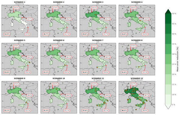
Figure 4 shows the MER for total CH₄ emissions across four regions (all of Italy, Northern Italy, Central Italy, and Southern Italy) for each network scenario, and averaged over the five truth scenarios. In Scenario 1, which includes only neighboring stations, Northern Italy exhibits a moderate constraint with MER, reaching 18.0 %. In contrast, the capacity of the network is slightly weaker in Central Italy (MER < 15 %), while Southern Italy remains essentially unconstrained, with MER as low as 3.9 %.

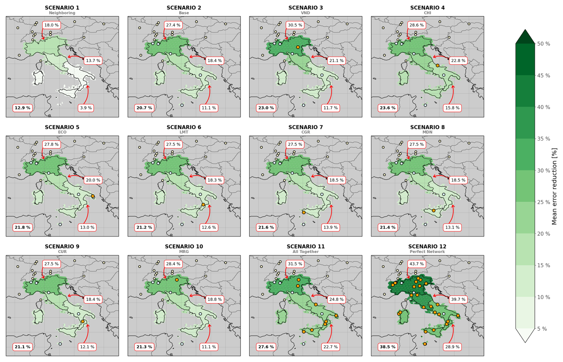
Figure 4 Spatial distribution of MER across Italy, shown for the whole country and separately for Northern, Central, and Southern Italy. The displayed MER is averaged over the five truth scenarios. For each region, the corresponding MER value is annotated in a box placed near its location, while the national value is displayed in bold in the lower-left corner of each panel. Stations in neighboring countries (Scenario 1) are marked with yellow circles. Existing ICOS stations in Italy (Scenario 2) are marked with blue circles. Additional stations introduced in subsequent scenarios are shown as orange circles.

Including the existing ICOS stations within Italy (Fig. 4, Scenario 2) markedly improves the agreement between posterior and true fluxes, raising MER by about 5 %–10 % across all regions. However, Southern Italy remains poorly constrained by the existing ICOS network compared to the other regions.

Analysis of individual candidate stations indicates that Mount Venda (VND) and Chieti (CHI) perform best, each achieving 1 %–2 % higher MER than other sites (Fig. 4, Scenarios 3 and 4). VND is particularly effective in Northern Italy, whereas CHI provides stronger constraints in Central and Southern Italy, outperforming all the other candidate stations in those regions. Other stations, such as Lecce (ECO) and Capo Granitola (CGR), also improve network performance reasonably. While ECO captures information about emissions both in Central and Southern Italy, CGR improves the coverage in Southern Italy.

Idealized expansion (i.e., adding all candidate stations in Scenario 11 and the full set of ICOS ecosystem stations in Scenario 12) provides substantial gains, with MER for all of Italy reaching 27.6 % and 38.5 %, respectively. While Northern and Central Italy shows similar results under Scenario 12, Southern Italy remains less constrained. This comparatively weak constraint can be attributed to three factors:

• Small flux signals: Enhancements observed at Southern stations are comparable to or lower than the model–data mismatch, limiting the inversion's ability to attribute them to specific sources. By contrast, larger enhancements at VND and CHI allow for clearer source identification.

• Geographical placement: Most Southern sites are not centrally located, reducing overlap between their footprints and the Italian landmass. Potenza (POT) is an exception, providing stronger coverage thanks to its central position (see ER and UR high values around POT in Fig. 3c and e) .

• Meteorological conditions: Prevailing winds in the region do not consistently transport emissions from inland areas toward the stations, restricting their effectiveness in detecting key sources.

The TUR results (see Fig. C1) are consistent with these findings. CHI and VND yield identical, and the largest, uncertainty reductions, exceeding those of other sites by approximately 4 %. VND has the strongest influence in Northern Italy, whereas CHI provides greater benefits in the rest of the country.

These results underscore the importance of the CHI and VND sites for constraining CH₄ emissions in Italy, identifying them as the strongest candidates for extending the ICOS network in the country. Behind CHI and VND, ECO and CGR are also good candidates.

3.2 Sensitivity to truth

Figure 5 shows MER for all truths, emphasizing the large variability of results one can infer using different truth scenarios. At the national scale, the MER is found to vary by up to 5 % around the mean (Fig. 5a, gray range), which is large compared to the differences between scenario results. The truth has such an importance because the posterior scaling factors typically remain unchanged compared to the prior (i.e., close to 1) over areas where there are no monitoring stations because of a lack of information. If the true scaling factors are also close to 1 over these areas, the agreement will appear to be large not because of constraints provided by the network, but because of randomness. For example, in second truth scenario, some grid cells have true scaling factors already close to 1 in Central Italy (Fig. S3, panel 2a). The posterior values also stay close to 1 because of a lack of observations, and the artificial agreement between the truth and posterior estimates leads to a good MER. By contrast, MER in the fourth truth scenario (Fig. 5c, purple rectangle) is notably low in Central Italy compared to the other truth scenarios, for most of the candidate stations. This arises because the fourth scenario includes a patch of high (randomly generated) scaling factors over this region in the true natural emissions, close to a patch of low values in Northern Italy (Fig. S3, panel 3b). Due to the lack of observational constraints, the system cannot properly disentangle these values, and the posterior scaling factors remain close to 1 on a large portion of Central Italy, leading to a small MER. These results highlight that a robust assessment can only be achieved by using an ensemble of truth scenarios that captures the spread of emission uncertainties.

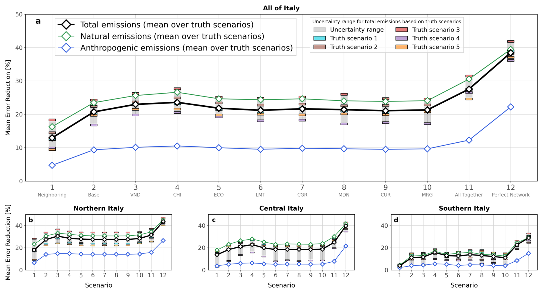
Figure 5 MER for each network scenario over all of Italy, Northern Italy, Central Italy, and Southern Italy. Black, green, and blue lines represent MER for total, natural, and anthropogenic emissions, respectively, averaged across all truth scenarios. The shaded area indicates the uncertainty range of MER for total emissions arising from different truth scenarios, while the colored rectangles show MER calculated for the individual truth scenarios.

On the contrary, results for TUR are not dependent on truth scenarios. This is because the posterior error covariance matrix in Eq. (4) is a function only of the error covariance matrices (i.e., the prescribed prior relative uncertainties, correlation lengths, and model-data mismatch) and the transport model (see Thanwerdas et al., 2025 and references therein).

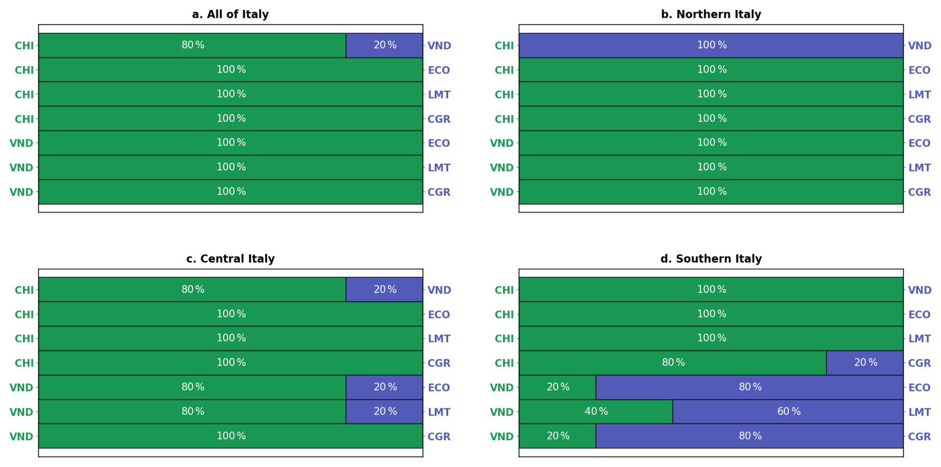
Figure 6 Pairwise comparison between network scenarios. In each comparison, the horizontal bar is divided into two sub-bars (green and blue). The green sub-bar (and its associated percentage) represents the fraction of truth scenarios in which adding the first station (green) yields a greater improvement in MER than adding the second station (blue). Conversely, the blue sub-bar (and its percentage) indicates the fraction of truth scenarios where adding the second station (blue) leads to a larger MER improvement than the first. For example, CHI outperforms VND in terms of MER for all of Italy in 80 % of the truth scenarios.

Because different truth realizations can yield different MER outcomes, it is important to assess how often one station provides stronger constraints than another, i.e., the probability that adding one station improves MER more than adding a different station. Figure 6 presents these pairwise comparisons. At the national scale, adding CHI outperforms VND in terms of MER for 80 % of the truth realizations (Fig. 6a, first line). This highlights the importance of using different truth scenarios. Using only one scenario could have resulted in preferring VND over CHI. In Northern Italy, VND consistently provides stronger constraints than CHI (100 % of the realizations) as well as any other station. In Central Italy, CHI almost always outperforms VND, while VND tends to be better than the remaining stations. In Southern Italy, CHI is consistently superior to both VND and the other stations. However, while averages over the truth scenarios suggest that ECO, Lamezia Terme (LMT), and CGR generally outperform VND in the South, a notable fraction of the realizations (20 %–40 %) indicate better performance for VND (Fig. 6d, three last lines). This highlights that, in some cases, VND can also provide stronger constraints than the Southern stations in Southern Italy.

These results confirm that CHI and VND would be the best choices to extend the ICOS network in Italy. In addition, it shows slightly stronger results in favor of CHI, although the difference is small.

3.3 Anthropogenic and natural emissions

Figures 5 and C2 present MER (averaged across all network scenarios) and TUR for total, anthropogenic, and natural emissions.

At the national scale, MER and TUR for anthropogenic emissions reach about 10 % and 15 %–20 %, respectively, across all candidate stations. These emissions are best constrained in Northern Italy, where they are most intense: adding VND (Scenario 3) increases MER to 15 % and TUR to nearly 20 %, representing the strongest performance in this region. In contrast, anthropogenic emissions remain poorly constrained in Central and Southern Italy, with both MER and TUR below 10 %. Compared to total emissions, the weaker performance for anthropogenic emissions arises from two main factors. First, separating natural and anthropogenic contributions in the observed signal is intrinsically difficult. Without additional constraints (e.g., isotopic information), the inversion relies only on spatial and temporal differences. When natural and anthropogenic emissions are co-located and occur simultaneously, the optimization process cannot effectively separate them, resulting in poor agreement between the posterior and true fluxes for each category. Second, anthropogenic emissions are assigned a shorter spatial correlation length in the prior error covariance (Sect. 2.3.1), following recent literature. While more realistic, this choice increases the number of degrees of freedom and thus the complexity of the inverse problem. In other words, the true scaling factors for anthropogenic emissions vary more spatially than those for natural and total emissions. As a result, constraining the higher heterogeneity of anthropogenic scaling factors with the same number of observations is more challenging, leading to poorer performance.

Natural emissions are therefore better constrained than anthropogenic emissions. They are more spatially diffuse and characterized by a larger spatial correlation length, making the metrics less sensitive to favorable wind conditions (i.e., transport from source regions to stations). Their performance closely follows that of total emissions, with MER values typically about 4 % higher across most regions, except in Southern Italy where they are nearly identical.

Across all regions, the conclusions for anthropogenic and natural emissions remain consistent with those for total emissions. Although anthropogenic emissions are only weakly constrained, CHI and VND consistently outperform the other sites across all categories, with VND performing best in Northern Italy and CHI in the remaining regions. The separation between anthropogenic and natural emissions is discussed further in Sect. 4.

3.4 Seasonality

As explained in Sect. 2.7, different sets of true scaling factors were generated for successive 10 d windows for both natural and anthropogenic emissions to account for a potential temporal variability in the associated uncertainties. This introduces a “true” seasonality in anthropogenic, natural, and total emissions that differs from the prior. We assess the inversion's ability to recover this true seasonality by analyzing the seasonal behavior of MER and TUR. Results are shown in Figs. 7 and C3, respectively.

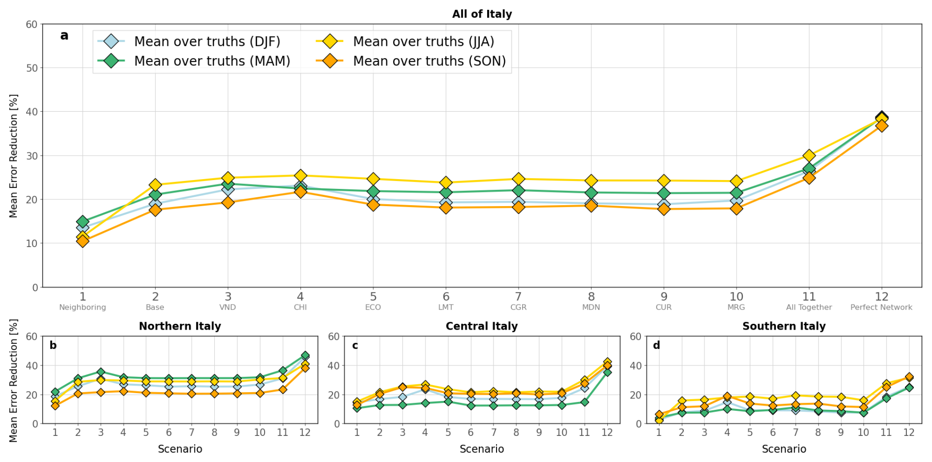
Figure 7 MER for each scenario over all of Italy, Northern Italy, Central Italy, and Southern Italy. Blue, green, yellow and orange lines represent MER for total emissions (mean over truth scenarios) in DJF (December–January–February), MAM (March–April–May), JJA (June–July–August) and SON (September–October–November), respectively.

To limit the number of abbreviations in this section, DJF, MAM, JJA, and SON are hereinafter also referred to as winter, spring, summer, and autumn, respectively. Seasonality can have a substantial influence on MER mainly through three drivers:

• Larger flux signal differences: The inversion system can more effectively attribute and locate underlying sources when (1) the station captures the emission signal and (2) the resulting signal difference between prior simulated values and assimilated pseudo-observations, caused by discrepancies between prior and true emissions, exceeds the model–data mismatch. For example, if the discrepancy between prior and true emissions peaks during winter and the signal can be adequately captured by the stations, a higher MER will be obtained during that season. However, when evaluating the performance averaged over multiple truth scenarios, this specific driver is neutralized. Because each scenario features a distinct random seasonal profile, averaging the performance eliminates the systematic influence of individual mismatches between prior and true emissions, thereby leaving only the influence of the other drivers introduced below.

• Wind speed and vertical convection: Seasonal shifts in wind speed and vertical convection directly alter atmospheric transport from source regions to monitoring stations, thereby influencing inversion performance. In winter, stronger synoptic winds extend the station footprints further upwind. While this wide, advection-dominated footprint allows the inversion to constrain a larger geographic area, it simultaneously dilutes the constraint's intensity. Conversely, weaker summer winds combined with intense vertical convection restrict the footprint to a more localized area. This concentrates the inversion's capability, likely maximizing error reduction near the station while reducing its influence on more distant regions.

• Wind direction: Seasonal variations in wind direction dictate whether a monitoring station is positioned downwind of the target source region. If the station is not downwind of the emissions during a specific season, the network's capacity to constrain those sources is effectively lost.

For most network scenarios, the highest MER values for total emissions are achieved during summer or spring across all regions. Because Eulerian frameworks, unlike Lagrangian frameworks (see Sect. 4), do not directly output footprint sensitivity maps, interpreting these results is inherently challenging due to the complex interplay between wind speed, wind direction, and vertical convection. Nevertheless, an interpretation can be proposed. The vigorous convective mixing characteristic of summer afternoons is likely a primary driver of the elevated MER values observed at both national and regional scales. Given our natural scaling factors exhibit large spatial correlation lengths, the enhanced constraint on emissions close to the stations in summer likely help to constrain broader regions sharing similar scaling factors. However, convective mixing alone cannot be the sole explanation. For instance, MER peaks during spring in Northern Italy but drops significantly during the same season in Central and Southern Italy, despite high convective mixing. In Northern Italy, this spring peak in 2018 was likely driven by stronger seasonal winds relative to summer. In contrast, for Central and Southern Italy, the lower spring MER is potentially tied to the specific meteorology of 2018, where strong, predominantly westerly winds limited the transport of inland emissions toward the monitoring sites. By summer, a shift to north-westerly winds allowed the stations to sample a greater fraction of inland emissions, thereby improving the constraint.

The TUR outcomes generally mirror those of MER, with one notable exception: autumn values align much closer to those of spring and summer than observed in the MER results. This relative improvement is likely driven by the highly variable wind directions across Southern and Central Italy during autumn 2018, which broadened the station footprints. While such wind variability does not necessarily improve MER, as it dilutes the peak emission signals and makes them less distinguishable, it might successfully reduce posterior uncertainty across a wider geographical area, thereby enhancing TUR.

Although seasonality affects both MER and TUR for individual network scenarios, the differences between scenarios show little seasonal variation; in other words, the seasonal influence is largely similar across all stations.

3.5 Sensitivity to model-data mismatch

We evaluate the impact of incorporating a non-uniform model–data mismatch in our analysis. For real stations, this mismatch is estimated using observations from the AVENGERS obspack data product. For candidate stations, where observations are unavailable, we rely solely on simulated values.

For the real stations, we first perform a forward simulation for the year 2018. Simulated values are then sampled and compared to observations to compute an initial model–data mismatch using the root mean square error (RMSE). This initial estimate is used to perform an inversion for 2018. Following this initial inversion, we recalculate the RMSE using the posterior mole fractions, which provides a refined estimate of the model–data mismatch at these stations, and then perform a new inversion using this updated estimate of model-data mismatch. The results of this second inversion are analyzed.

For the candidate stations, a forward simulation for 2018 is conducted. In this case, we use the standard deviation of the simulated values at each station as a proxy for model–data mismatch. This approach was validated against real stations, showing a strong correlation with the RMSE-based estimates (r=0.96). We also tested alternative methods based on a moving average (7 d and monthly) of the simulated values, following Villalobos et al. (2025), but found that it yielded weaker correlations. Such differences might be related to the fact that CO₂ concentrations often show strong hourly fluctuations driven by the diurnal cycle of photosynthesis and respiration, unlike CH₄. Therefore, a 7 d moving average may be suitable for CO₂ but less representative for CH₄.

Results obtained using the non-uniform model–data mismatch are provided in the Supplement. Most inferred mismatches exceed 20 ppb (Table S1), with a mean value of 31 ppb, indicating lower confidence in the measurements than initially expected. JFJ exhibits the smallest mismatch (14 ppb), whereas IPR and IT-BFt show the largest values (75 ppb). Large model–data mismatches suggest difficulties in capturing the observed variability at these stations. In particular, observations at IPR are known to be challenging for transport models due to the complex surrounding terrain. The CHI model–data mismatch (46 ppb) is estimated to be larger than that of VND (35 ppb), giving a slight advantage to VND compared to the experiments with a uniform mismatch. Using these new estimates of model-data mismatches, both MER (Table S2, Figs. S4 and S7) and TUR (Table S3, Figs. S5 and S8) decrease by 2 %–6 % compared to the experiments assuming a uniform model–data mismatch.

Nevertheless, the conclusions drawn in the previous sections remain unchanged: Scenarios 3 (VND) and 4 (CHI) continue to be the optimal choices for all of Italy when comparing MER and TUR values to other scenarios, with CHI retaining a marginal advantage.

4 Discussion

In this study, we conducted an extensive analysis of network scenarios in Italy using OSSEs and inverse modelling. One of the main added values of this work is the creation of multiple truth scenarios, which limits the influence of randomness. Nonetheless, our methodology also entails several caveats and limitations. Most of these could be addressed with additional simulations, but this would significantly increase the computational cost of the analysis.

A first limitation lies in the assumption of perfect knowledge of prior relative uncertainties and correlation lengths in the inversion setup. In reality, these parameters can only be approximated. Introducing a mismatch between the assumed values and those used to generate the true scaling factors would have affected the optimal solution and reduced performance (Steiner et al., 2024a). However, we expect this reduction would have occurred uniformly across network scenarios, leaving the main conclusions regarding VND and CHI unchanged.

Similarly, the model–data mismatch applied to perturb the synthetic observations was prescribed to follow a normal distribution, which may not hold for real data. Deviations from this assumption could further degrade inversion performance. It is therefore important to understand that these results are produced with perfect knowledge.

We performed the OSSEs for the year 2018 to ensure consistency with Villalobos et al. (2025). Although dominant winds generally remain stable from year to year at the national scale, local variations can occur that may alter the emission signals captured by the stations and, consequently, the results. A more comprehensive picture would require reproducing this study over multiple years. However, the computational demands of such an analysis remain a major limitation and make it difficult to implement in practice.

We assumed an inlet height of 100 m for most lowland candidate stations, implying the construction of tall towers at these sites in addition to existing infrastructure. This sampling height was chosen because ICOS continental stations typically operate at such elevations to reduce local influences, increase model representativeness, and enhanced sensitivity to regional fluxes. Our results should therefore be interpreted in light of this assumption. Sampling at higher levels is unlikely, as it would drastically increase costs while likely providing limited added value, given that local influences are already dampened at 100 m. Moreover, because only afternoon observations are assimilated, the boundary layer is generally well mixed, further reducing the benefit of sampling at greater heights. In contrast, sampling at lower heights, which is more likely in practice, could increase model–data mismatch and reduce the spatial footprint, potentially leading to lower performance. Nevertheless, this effect may remain limited during the afternoon, when vertical mixing reduces differences between observations sampled at 100 m and at lower levels. Note, however, that these considerations are likely site-dependent and would require further investigation through dedicated OSSE studies conducted at much higher spatial resolution and for different inlet heights at the most promising sites identified here. Importantly, CHI only began operating in March 2026, after the start of this study. At that time, the projected inlet height was 50 m, and this value was therefore retained in our analysis. However, the station was ultimately equipped with an inlet height of 15 m. This decision was primarily driven by practical considerations, including funding limitations and, more importantly, regulatory constraints associated with the station's location within an environmentally protected area. The time required to address these constraints was not compatible with the duration of the funded project. Consequently, it was decided to proceed, in this initial phase, with a sampling height of 15 m. As a result, the first observations from CHI may provide fewer constraints than those estimated in this study. Discussions are currently ongoing regarding a potential future extension of the inlet height to 50 m.

In principle, the Eulerian-model-based methodology introduced here could be extended to determine the optimal location of a measurement station over the whole domain. However, such an application would require as many inversions as grid cells in the model domain, and considerably more if multiple sampling heights and truth scenarios were also tested. At present, this is computationally infeasible, and analyses must remain restricted to a manageable set of candidate stations. Notably, the inclusion of multiple truth scenarios already demanded significantly greater computational resources than are typically required for OSSEs.

Although a Eulerian model is employed in this work, Lagrangian models can also be used to conduct network expansion studies. Lagrangian frameworks offer several advantages over Eulerian frameworks, but also have notable limitations. In Lagrangian frameworks, footprints can be readily computed, providing an intuitive and effective means of investigating the spatial and temporal sensitivity of measurements to surrounding fluxes. Once computed, these footprints can be reused, enabling multiple site configurations to be tested with negligible additional computational cost. Moreover, the evaluation metrics introduced in this work can be derived just as easily within a Lagrangian framework. Using the footprints, the full Jacobian of the observation operator can be computed efficiently, making the direct application of Kalman filter equations (i.e., an analytical inversion) a natural choice, in contrast to the ensemble-based approach adopted here. However, the analytical approach does not scale well to very large control or observation vectors, as it requires inversion of the associated error covariance matrices. While it is possible to assimilate large numbers of observations sequentially under the assumption of uncorrelated errors, the computational cost increases rapidly with the number of optimized variables. This effectively limits the dimensionality of the inversion problem and, consequently, the amount of information that can be extracted from the observations. For this reason, in the present case study focusing on surface stations, the primary advantage of a Eulerian framework lies in its ability to optimize emissions at high spatial (e.g., model resolution) and temporal (e.g., daily or weekly) resolution. In addition, Eulerian frameworks are well suited for the assimilation of satellite data, which requires the calculation of column-averaged mole fractions using averaging kernels. In contrast, Lagrangian models require particles to be released throughout the atmospheric column to estimate sensitivities of column-averaged mole fractions to emissions, substantially increasing computational demand and making their application to satellite data inversions more restrictive.

In this work, we employed two complementary evaluation metrics: the TUR and the MER. While these two metrics are highly correlated (experiments with a high TUR often exhibit a high MER and vice versa), the correlation is not perfect, as shown in Fig. S9 in the Supplement. For instance, TUR values in autumn and spring are similar for total emissions in Northern Italy, yet the corresponding MER values can differ by as much as 10 % (see Tables B1 and B2), which is substantial. In our experiments, such decorrelation between the two metrics occurs mainly when seasonal dependence is introduced. When it is removed, the correlation between TUR and MER becomes much stronger. As discussed earlier, variable wind conditions can improve spatial coverage around the station, leading to a high TUR. However, this same variability can make it harder to localize the signal accurately, resulting in a low MER. Thus, a trade-off exists between TUR and MER, underscoring the importance of considering both metrics when evaluating network performance. In practical, real-data applications, MER cannot be computed because the true emission values are unknown. Although TUR generally provides a reasonable proxy for assessing the agreement between posterior and true emissions, low posterior uncertainties do not necessarily imply that the mean posterior estimates are accurate. This emphasizes the importance of reporting the full range of plausible estimates rather than central estimates only.

Villalobos et al. (2025) conducted a similar study focusing on CO₂ rather than CH₄, using a Lagrangian-based framework. The candidate stations were identical, with the same inlet heights. Although they did not use the same evaluation metrics, they both quantified the uncertainty reduction and the agreement between posterior and true CO₂ fluxes, using a single truth scenario. Despite using inversion setups different from ours, they also found that CHI provides the strongest constraint among the candidate stations, with VND being the second-best site in terms of uncertainty reduction. When two stations were added to the network, the CHI–ECO combination yielded the best performance. This result is somewhat counterintuitive, as adding ECO alone provided weaker constraints, both in terms of agreement with true fluxes and uncertainty reduction, than VND. This suggests that station synergies cannot be simply inferred from the sum of individual station impacts. Although we could not test multi-station combinations due to computational limitations, the strong agreement between our single-station results and those of Villalobos et al. (2025) indicates that the overall outcome would likely be similar. These findings reinforce that CHI is the most promising candidate for expanding the Italian observation network. CHI appears to be strategically located to capture key transport patterns and flux signals influencing both gases, highlighting its importance as a potential addition to the ICOS network.

It is important to note that, except for scenarios 11 and 12, which feature multiple stations, differences in results between network scenarios are small, indicating that no single station can largely improve coverage in Italy. Although CHI and VND perform slightly better individually, it is only when multiple stations are strategically placed that the network can effectively constrain fluxes.

Additionally, substantially improving constraints on anthropogenic emissions using CH₄ measurements alone appears challenging. In this study, we adopt realistic conditions, including a shorter error correlation length for anthropogenic emissions. Even when adding the optimal station locations identified here, improvements in anthropogenic emission estimates remain limited. While the results show relatively good performance for total emissions, one of the primary objectives of top-down approaches is to complement bottom-up estimates by providing comparable information to better quantify anthropogenic emissions. Our results, consistent with previous literature, indicate that achieving this goal requires additional observational constraints, such as isotopic measurements or co-emitted species. Without such information, the ability to accurately constrain anthropogenic emissions in Italy will remain limited.

5 Conclusions

In this study, we conducted Observing System Simulation Experiments (OSSEs) to assess the potential expansion of the ICOS monitoring network in Italy for CH₄. This work complements the recent study by Villalobos et al. (2025), which focused on CO₂. Our results show that CHI and VND are the most promising candidate stations for improving emission constraints in Italy, with CHI having a slight advantage. While CHI provides stronger constraints in Central and Southern Italy, VND is particularly effective in Northern Italy. Importantly, these stations are also the most likely to be implemented in the future.

To evaluate the impact of adding these stations, we introduced two complementary metrics: the mean error reduction (MER) and the total flux uncertainty reduction (TUR). These metrics were applied to estimate the effect of new stations on total, anthropogenic, and natural emissions, both annually and seasonally, for three Italian regions as well as the entire country.

We also tested multiple truth scenarios to account for randomness in generating both true emissions and synthetic observations. The analysis shows that randomness strongly influences the results, highlighting the limitations of relying on a single truth scenario. In addition, we quantified the effect of assuming a non-uniform model–data mismatch and found that, in this case study, it did not significantly alter the conclusions.

The methodology we present can be readily applied to other Eulerian models and adapted to different countries or regions. We therefore strongly recommend adopting a similar approach, using the robust and informative metrics introduced here, and employing an ensemble of truth scenarios to reduce the influence of random effects. While computationally demanding, this type of OSSE study offers valuable guidance for decision-makers and atmospheric scientists when selecting candidate sites and optimizing observational coverage.

However, this work also demonstrates that the network, even when extended with the best candidate site, has limited potential to constrain anthropogenic emissions. This remains one of the primary objectives of inverse modelling, as the design and implementation of effective mitigation policies depend on robust quantification and understanding of these emissions.

Although we identified optimal locations among a set of candidate sites, a substantial number of additional stations would still be required to substantially reduce the discrepancy between bottom-up and top-down estimates. In this study, we only evaluated the extension of the surface CH₄ monitoring network. Further constraints could help improve the partitioning between natural and anthropogenic sources, such as isotopic measurements or co-emitted species (e.g., ethane).

These approaches warrant investigation in future OSSEs to assess whether deploying new stations or enhancing existing ones with additional observational capabilities (e.g., isotopes or co-emitted tracers) would be more effective. Importantly, a national capacity for stable isotopic carbon measurements has been established in Italy through the deployment of Cavity Ring-Down Spectroscopy (CRDS) isotopic analysers at CMN, POT, LMT, and LMP. Moreover, ethane measurements were initiated at CMN in 2023 within the framework of ACTRIS (Aerosol, Clouds and Trace Gases Research Infrastructure). Satellite data also holds strong potential for covering regions that are poorly sampled by ground-based stations, providing information at finer spatial scales. Although satellite observations are subject to larger uncertainties and are more challenging to assimilate into transport models, they could complement surface measurements and substantially improve estimates of total, natural, and ultimately anthropogenic emissions.

Appendix A: Surface stations

Table A1 List of candidate stations.

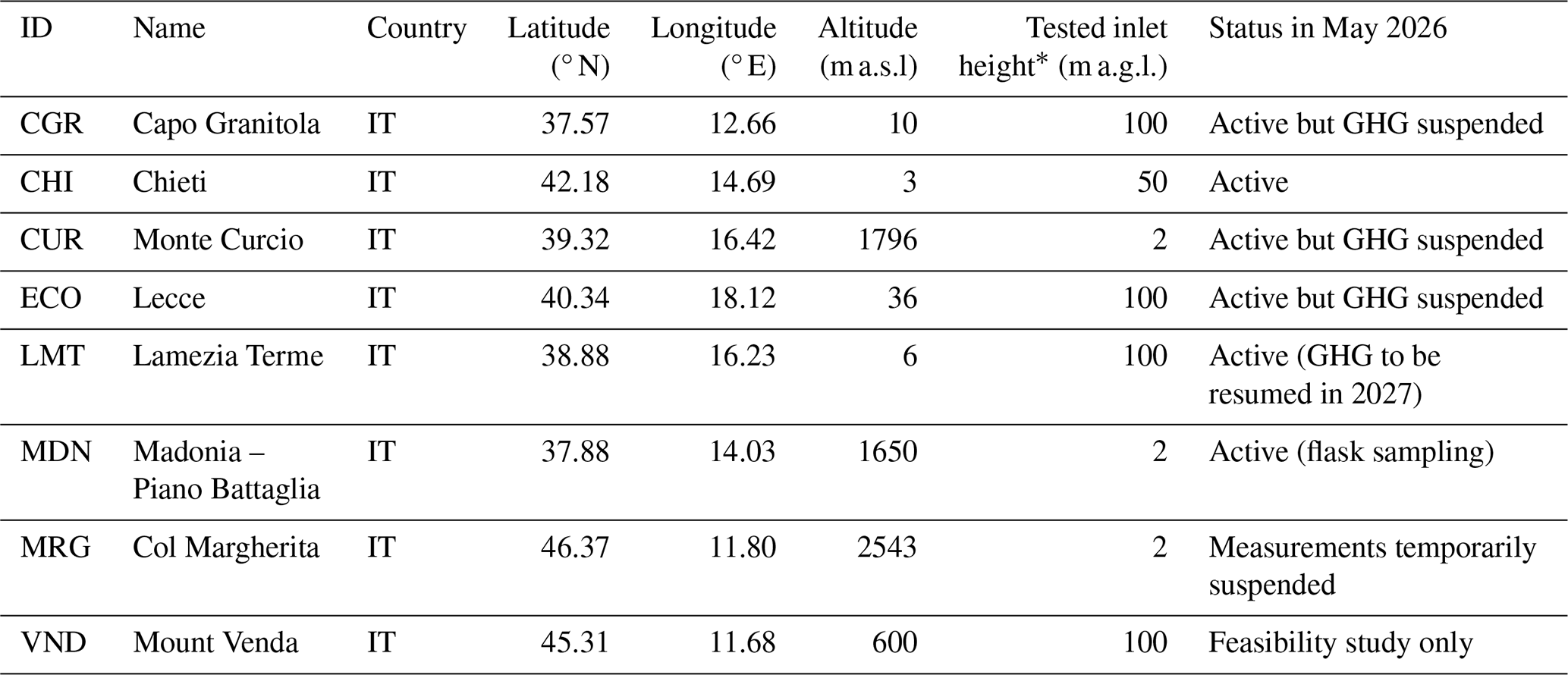
^∗ Tested inlet height denotes the inlet height used to generate the synthetic observations assimilated in this study. It represents a preliminary estimate for a potential ICOS station that could operate at this location.

Table A2 List of existing ICOS Atmosphere sites in Italy and in the surrounding countries.

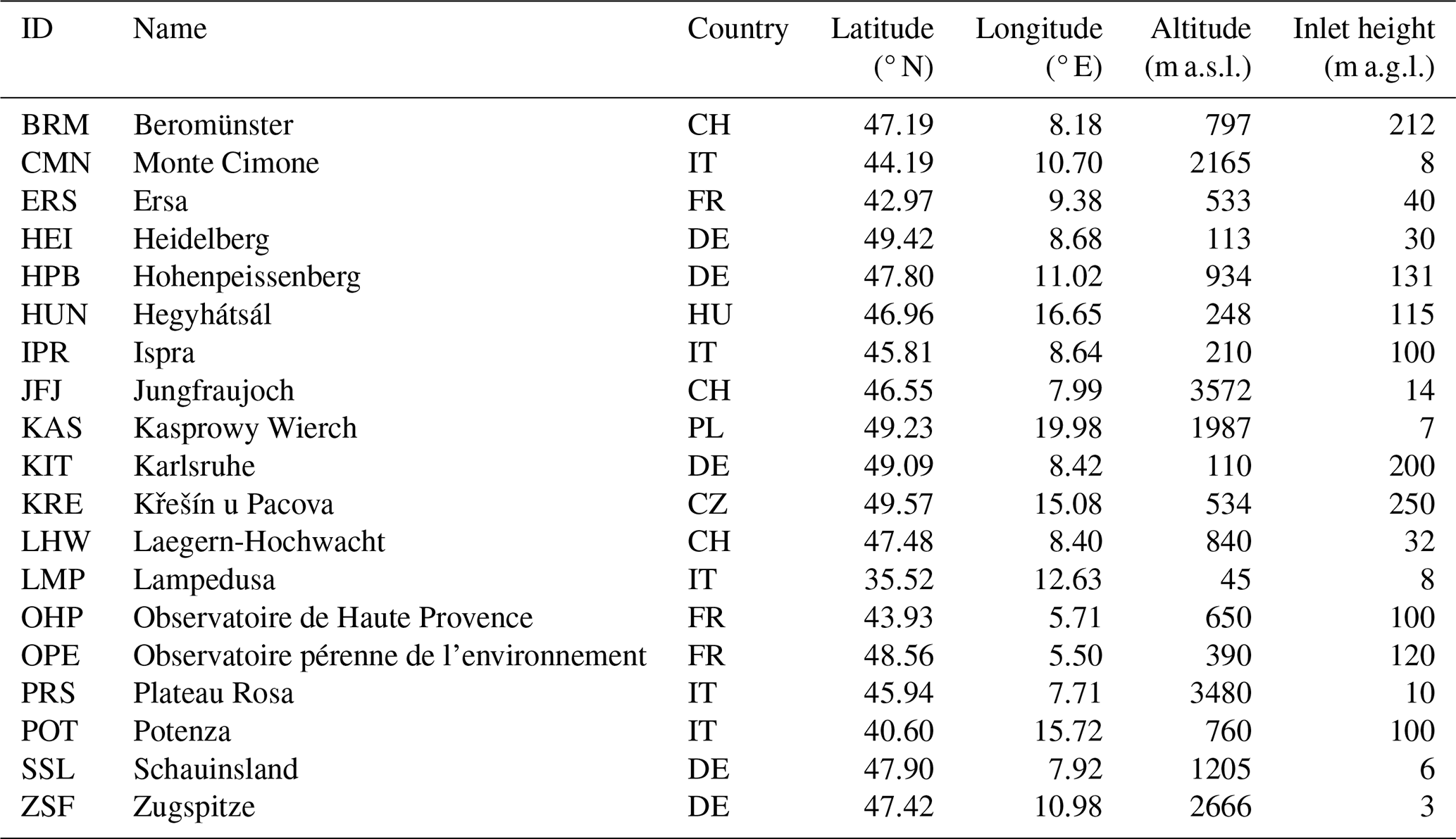
Table A3 List of ICOS ecosystem surface stations. The inlet height provided here represents a preliminary estimate for a potential ICOS station that could operate at this location.

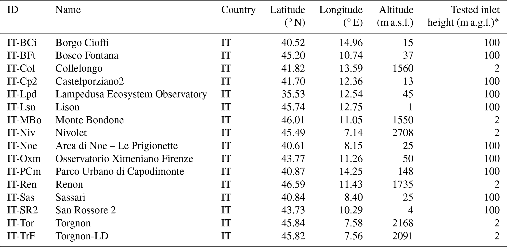
^∗ Tested inlet height denotes the inlet height used to generate the synthetic observations assimilated in this study. It represents a preliminary estimate for a potential ICOS station that could operate at this location.

Appendix B: MER and TUR values

Table B1 MER values for all network scenarios, regions, emission categories and seasons, averaged over all truth scenarios.

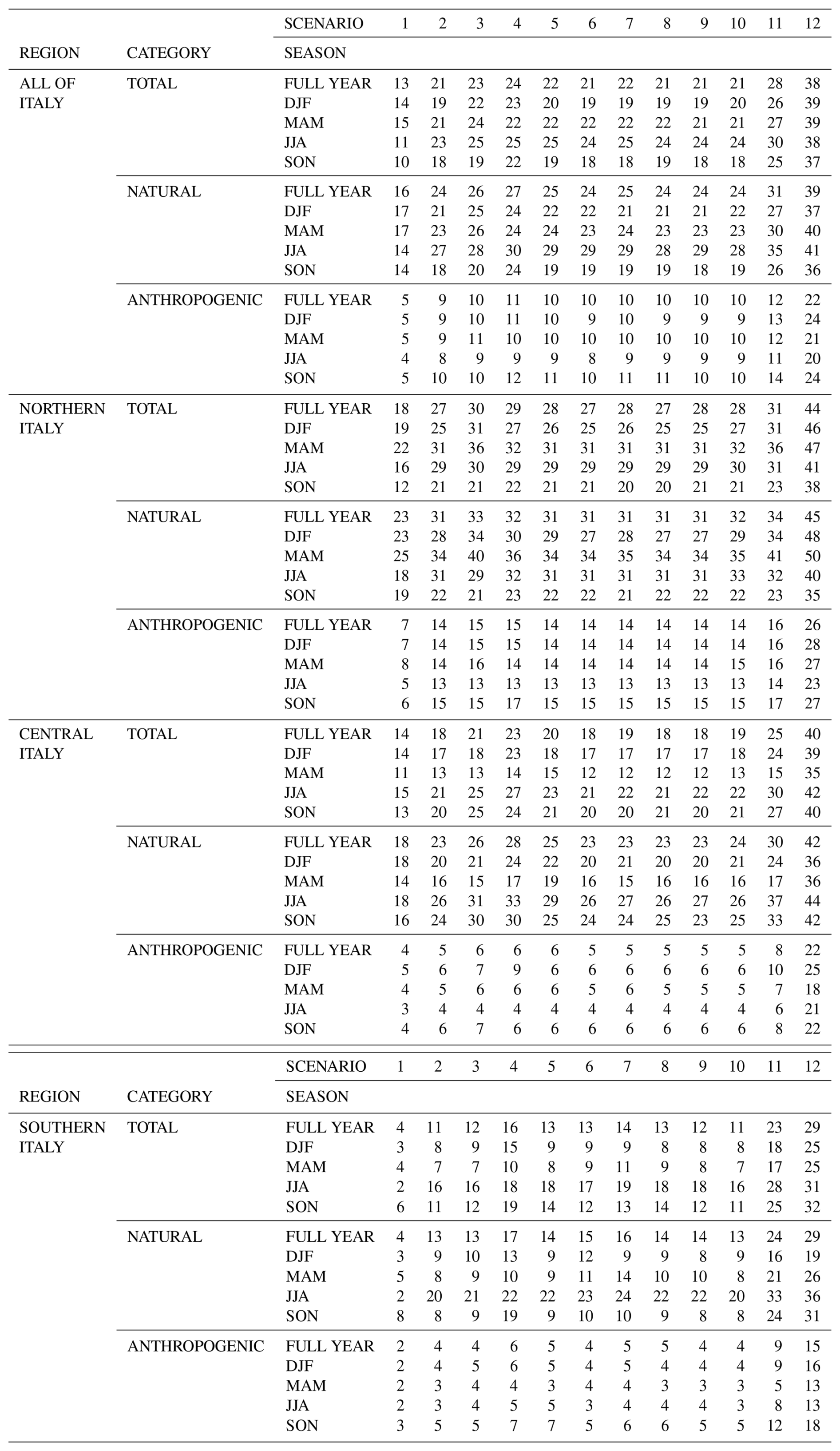
Table B2 TUR values for all network scenarios, regions, emission categories and seasons.

Appendix C: Additional figures

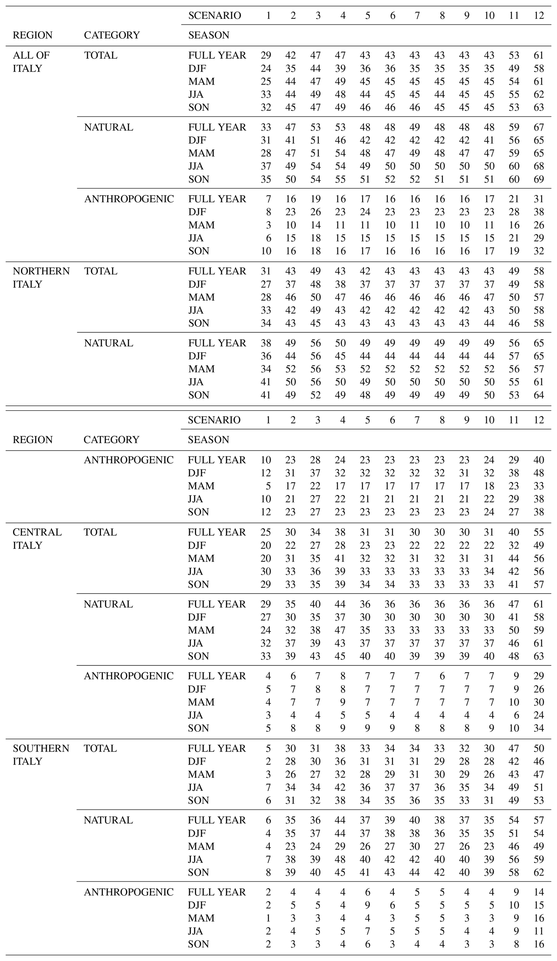
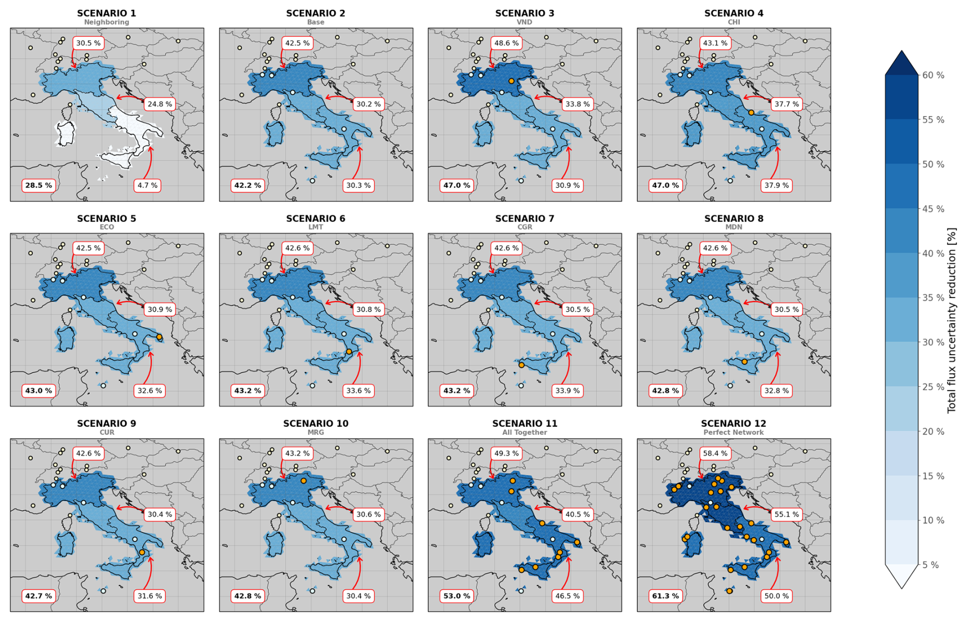
Figure C1 Spatial distribution of TUR across Italy, shown for the whole country and separately for Northern, Central, and Southern Italy. For each region, the corresponding TUR value is annotated in a box placed near its location, while the national value is displayed in bold in the lower-left corner of each panel. Stations in neighboring countries (Scenario 1) are marked with yellow circles. Existing ICOS stations in Italy (Scenario 2) are marked with blue circles. Additional stations introduced in subsequent scenarios are shown as orange circles.

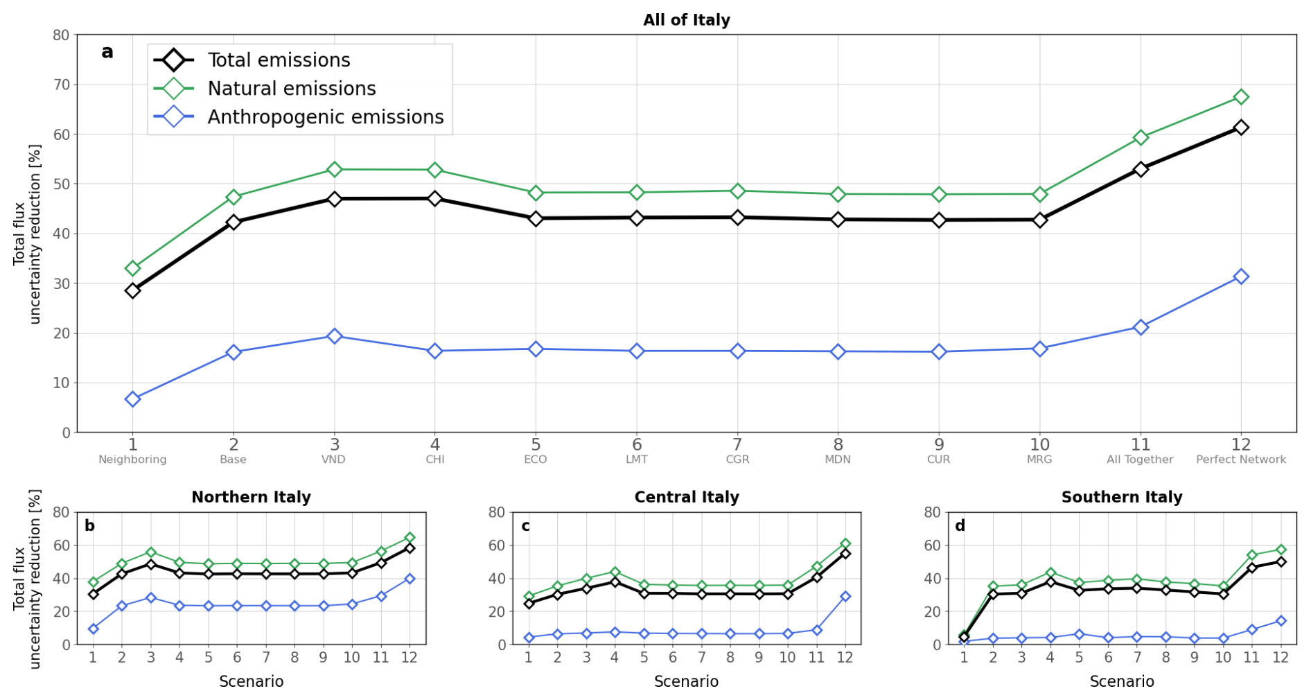
Figure C2 TUR for each network scenario over all of Italy, Northern Italy, Central Italy, and Southern Italy. Black, green, and blue lines represent TUR for total, natural, and anthropogenic emissions, respectively.

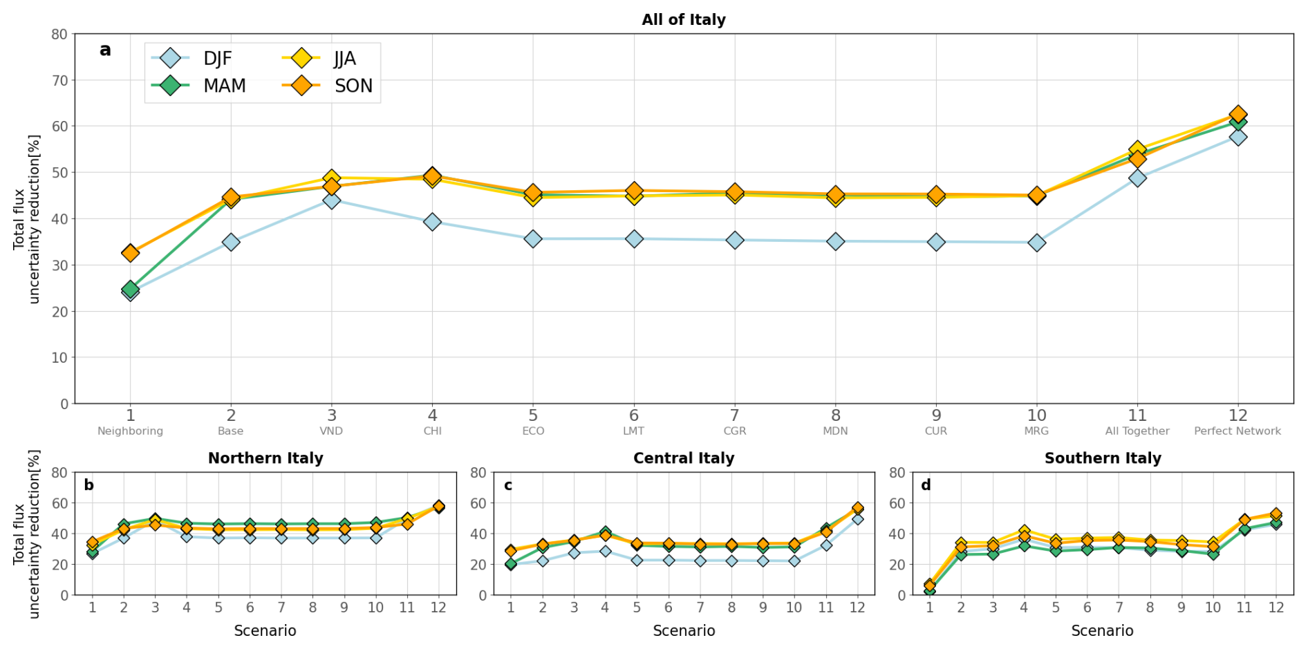
Figure C3 TUR for each scenario over all of Italy, Northern Italy, Central Italy, and Southern Italy. Blue, green, yellow and orange lines represent TUR for total emissions in DJF (December–January–February), MAM (March–April–May), JJA (June–July–August) and SON (September–October–November), respectively.